Self-organized criticality in boson clouds around black holes

Abstract

Boson clouds around black holes exhibit interesting physical phenomena through the Penrose process of superradiance, leading to black hole spin-down. Axionic clouds are of particular interest, since the axion Compton wavelength could be comparable to the Schwarzschild radius, leading to the formation of “gravitational atoms” with a black hole nucleus. These clouds collapse under certain conditions, leading to a “Bosenova”. We model the dynamics of such unstable boson clouds by a simple cellular automaton and show that it exhibits self-organized criticality. Our results suggest that the evolution through the black hole Regge plane is due to self-organized criticality.

I Introduction

Modern particle detectors are typically associated with very high energies, like the current design of the LHC with 8 TeV center of mass energy. The need for having high energies is obvious if the particles to be discovered — like the Higgs — have a substantial rest mass or, conversely, a tiny Compton wavelength.

Interestingly, for (QCD-)axions Peccei and Quinn (1977); Weinberg (1978); Wilczek (1978) the situation may be reversed: the rest mass of axions can be tiny, while their Compton wavelength can be substantial. More precisely, the axion Compton wavelength can be of the same order of magnitude as the Schwarzschild radius of a stellar mass black hole. Thus, at least in principle, black holes can serve as particle detectors for axions Arvanitaki et al. (2010); Arvanitaki and Dubovsky (2011). This idea has engendered a lot of recent interest Acharya et al. (2010); Marsh and Ferreira (2010); Panda et al. (2011); Dubovsky and Gorbenko (2011); Marsh (2011); Dubovsky et al. (2011); Kodama and Yoshino (2011); Cardoso et al. (2011); Marsh et al. (2011); Horbatsch and Burgess (2011); Alsing et al. (2011); Amaro-Seoane et al. (2012).

The present work is based on the working assumption that suitable axions exist in our Universe (we shall be more precise what “suitable” means in the body of the paper). In that case an axion cloud forms around a rotating black hole, and the combined system black hole/axion cloud can be thought of as a gigantic “gravitational atom”, with the black hole playing the role of the nucleus and the axion cloud playing the role of the electrons.

As explained in Arvanitaki and Dubovsky (2011), the dynamics of this “gravitational atom” is governed by the Penrose process of superradiance Penrose (1969). This process leads to exponential growth of the occupation numbers of the “atomic” levels, i.e., the formation of an axion Bose–Einstein condensate. The energy required for the formation of this condensate is extracted from the black hole, which thereby spins down and also loses some of its mass $M$. In fact, the black hole parameters $(M,a)$ move on a Regge trajectory, where $a\in[0,1]$ is the Kerr parameter. Eventually, when the attractive axion self-interactions become stronger than the gravitational binding energy, the axion cloud collapses — a “Bosenova” occurs.

The aim of our present work is to map relevant aspects of the dynamics of the black hole/axion cloud system to a simple cellular automaton, and to show that it exhibits self-organized criticality. If this conclusion holds also for more realistic cellular automata it would mean that self-organized criticality governs an essential part of the dynamics of gravitational atoms.

This paper is organized as follows. In section II we review some preliminaries, namely crucial properties of self-organized criticality and the black hole/axion cloud system. In section III we present the working assumptions of relevance for our cellular automaton and argue to what extent they are plausible. In section IV we present results based upon computer simulations implementing this specific cellular automaton. In section V we summarize and point to open issues.

II Preliminaries

II.1 Self-organized criticality

The concept of Self Organized Criticality (SOC) was proposed as an organizing principle of Nature, as it was realized that numerous spatial extended systems, in physics, biology, social media and economics, exhibit a number of properties which may be shortly characterized as flicker noise for the temporal evolution and self-similar (fractal) behavior for the spatial evolution Bak et al. (1988). Ever since this seminal paper, the analytical and numerical methods developed to be able to tackle SOC in various contexts have led to progress in understanding the nonlinear dynamics of complex, interacting systems. It is expected that SOC develops in slowly driven interaction dominated threshold systems and it has been shown that this state is an attractor of the dynamics of such systems (see for instance Pruessner (2004) and references therein).

Due to the complex interactions between its constituents, after a transitory phase in its evolution, the system exhibits what may be called a phase transition to a state characterized by the absence of a critical length scale, i.e., in this state all lengthscales are relevant.

The archetypal SOC system is driven by an external force with a very large characteristic timescale and the system evolution is determined by local rules, i.e., only near-neighbor interactions are considered Sornette (2000); Pruessner (2004). One important point to make is that this external driver is not artificial/conscious but is intrinsic to the physics in the system. This property of SOC is unlike the phase transitions in an Ising type system, where the phase transition is acquired by a conscious tuning of parameters to a critical value.

Because this line of research is still in its infancy and due to the associated analytical complexity, analysis of such systems relies heavily on numerical methods and so they have become intertwined in an inseparable way. It is difficult to enumerate properties of SOC without relating them to the way they are simulated in computer experiments.

Systems which exhibit SOC are discrete (in general modelled by lattice models). The interaction between constituents are usually nearest neighbor-like and governed by local rules and are modelled as interaction between sites in a lattice, such that if one site receives an information, only a few other selected sites have access to this information. The entire system is subjected to an infinitely slow external drive and due to this drive and the complex interaction, the onset of SOC usually occurs when all the sites in the lattice host a near-threshold value of some parameter. If the threshold is reached, the system becomes subjected to different rules of evolution (critical flow) which allow information to be transmitted not only locally, but across all lengthscales. If one site has reached threshold and sends information to the next site, this next site might also reach threshold and so on. The avalanches of information from one seed site to a final site (i.e. where the threshold condition is no longer satisfied) form an event. The size of an event is the total number of avalanches occurring from one seed site. Natural systems that reach SOC maintain it for an indefinite time as long as the external driver keeps acting. This equilibrium state is maintained by a balance between driving and dissipation, which occurs at the boundaries or in the bulk.

The way that SOC was historically “detected” in Nature was due to the properties exhibited by observables of the system. These observables show a powerlaw distribution of values. It was shown Sornette (2000); Pruessner (2004) that, for a system in SOC, the distribution function $D(s)$ of some parameter $s$ is given by

$$D(s)=as^{-\tau}\mathcal{G}\left(\frac{s}{bL^{\sigma}}\right),$$ (1)

where $\mathcal{G}(x)$ is the universal scaling function for a given universality class of systems, $a$ is a system specific constant, $\tau$ is the critical exponent, $b$ is a system dependent amplitude, $L$ is the system spatial size and $\sigma$ is determined by the physical dimension of the parameter $s$. A very useful feature of SOC is that if the distribution of another observable, say $y$, is considered, then $D(y)$ will be equivalent to Eq. (1), with $s$ replaced by $y$ and different parameters $a$, $\tau$, $b$ and $\sigma$, but the same scaling function $\mathcal{G}$.

This is conceptually a powerful tool for observational purposes, in cases where it proves easy to record $D(s)$, but difficult to record a perhaps more interesting distribution $D(y)$.

An example of a system in SOC and a discussion of the properties emphasized above is given in the Appendix.

II.2 Massive boson instabilities near a rotating black hole

It has been shown Arvanitaki and Dubovsky (2011); Kodama and Yoshino (2011); Zouros and Eardley (1979) that the presence of bosons near a rotating black hole (BH) will lead to the formation of a boson cloud (BC) around the BH if a series of conditions are met. This BC-BH system is analogous to an atom. The cloud is being continuously fed with bosons due to the superradiance phenomenon. At some point, when the number of bosons in the cloud is too large, the nonlinearities in the BC lead to an unstable behavior and the cloud goes through a Bosenova-type event.

The conditions for this chain of events to occur refer to a set of parameters characterizing both the boson and the BH, $\{M,\omega_{h},\mu,\omega_{R},m\}$, where $M$ and $\omega_{h}$ are the mass of the BH and the angular velocity at the horizon, respectively, and $\mu$, $\omega_{R}$ and $m$ are the mass of the boson, angular velocity of the associated wavepacket and “magnetic” quantum number of the boson. The first condition requires that a boson exists such that its associated Compton wavelength, $\lambda_{b}$, is approximately equal to the characteristic size of the BH, $R_{g}$ (the Schwarzschild radius). It was shown that the QCD axion can satisfy this condition [in e.g. Arvanitaki and Dubovsky (2011)]. Superradiance, i.e., continuous feeding of the cloud with “free” bosons, the phenomenon analogous to the Penrose process for fields, occurs if the superradiance condition is met, namely if $\omega\in[0,\omega_{h}m]$. Once superradiance sets in, the topology of the growing cloud is given by a frequency $\omega_{R}$, which satisfies the superradiance condition and is the frequency of hydrogenic-like bound levels. Growth of the BC, instability and subsequent Bosenova occur if the frequency associated to the boson as it interacts with the BH has a very small imaginary part, $\Gamma_{g}$, such that the frequency describing the wavepacket in the potential well of the BH is $\omega=\omega_{R}+\imath\Gamma_{g}$. The parameter $\Gamma_{g}$, giving the growth of the BC, is a function of the set of parameters mentioned above and it exhibits a maximum for specific values of these parameters Arvanitaki and Dubovsky (2011).

We are now in the position to define the “suitable axion” mentioned in the Introduction. This axion is a boson which possesses physical characteristics such that $\lambda_{b}\simeq R_{g}$, $\omega_{R}\in[0,\omega_{h}m]$ and, in the potential well of a BH, exhibits a growth rate $\Gamma_{g}$ which is very small, $\omega_{R}\gg\Gamma_{g}$. The growth rate also depends on details of the bound system, such as the hydrogenic-like quantum numbers, taken here such that $\Gamma_{g}$ has its maximum possible value. We assume that this boson exists and give a general outline of the dynamics of the BC-BH system. Superradiance sets in and the number $N$ of such bosons in the vicinity of the BH is amplified, in the linear limit, as

$$\frac{dN}{dt}=\Gamma_{g}N.$$ (2)

However, during this amplification more complex processes occur. Most importantly, the nonlinearities start increasing and the bosons begin to interact with each other. The end result is that the number of axions present in the cloud is reduced, with a rate $\Gamma_{d}$ ($d$ from dissipation), where $\Gamma_{d}\ll\Gamma_{g}$. For our purposes, Eq. (2) can be naively modified as

$$\frac{dN}{dt}=\Gamma_{g}N-\Gamma_{d}N.$$ (3)

Even in this very simple description it is possible to recover some of the qualitative results derived rigorously in Arvanitaki and Dubovsky (2011). Since dissipation does not equilibrate growth, the number $N$ of bosons grows until the back-reaction on the frequency $\omega_{R}$ is such that the shape of the cloud departs from hydrogenic (nonlinear limit). This has been shown Arvanitaki and Dubovsky (2011); Kodama and Yoshino (2011) to occur when

$$\epsilon\equiv\frac{M_{BC}}{M_{BH}}=10^{-4},$$ (4)

where $M_{BC}$ is the mass of the boson cloud.

The cloud grows further, but in a nonlinear regime, until the nonlinearities in the boson self interaction potential are too large and the cloud is no longer stable. A large percentage of the cloud is supposed to collapse Arvanitaki and Dubovsky (2011); Kodama and Yoshino (2011) (critical limit). This collapse occurs on a timescale of $r_{g}$ of the BH, meaning that from the moment the critical limit has been reached, it takes $r_{g}$ units of time until a significant part of the cloud collapses into the BH.

The subtlety here is that this process occurs following an avalanche of information spreading on all lengthscales accessible to the system (i.e. with an upper bound given by the system size).

If the superradiance condition is still met, the cloud regrows within the same parameter space $\{M,\omega_{h},\mu,\omega,m\}$. In a plot of the BH spin vs. $M\mu$ (a Regge plot, Arvanitaki and Dubovsky (2011), their Fig. 3), the subsequent collapses and regrowths, with the same values of the parameters that initially satisfied the superradiance condition, resemble an almost straight line on which the systems wanders (Regge trajectories). It stays on this line for tens to hundreds of $e$-fold times of boson cloud growth, i.e. for tens to hundreds of Bosenovas. When the superradiance condition is no longer met with the initial parameters, the system makes a transition to another set of parameters (i.e., a new line on the Regge plot) which are again superradiant and analogous dynamics occurs.

III Cellular automaton for boson cloud around black holes

We want to map the dynamics of BC-BH system into SOC. As was mentioned previously, the concept of SOC and the simulation of SOC are intimately connected and the only contained way to map the BC-BH dynamics to SOC is to simultaneously discuss the computer simulation associated with this analysis. SOC simulations are generally done using Monte Carlo methods on discrete grids, and we will focus on a Cellular Automata (CA) approach. The CA is a “machinery” which stores values of a parameter on a discrete grid and evolves these values in time and space according to simplistic rules designed to mimic a real phenomenon Bandman (2008).

The CA used in the remainder of this paper is 2-dimensional cartesian grid, of size $L_{x}\times L_{y}$. While this undoubtedly simplifies the numerical effort, there is also strong physical argumentation in favor of considering a 2D grid (instead of a 3D grid). The BH has a significant spin, the quantum numbers of the atom are fixed (by assumption of the “suitable axion”) and the orbits are Keplerian, which means that angular momentum is conserved thus leading to planar motion.

Three questions then arise: 1) what is the quantity which will be placed on the grid, 2) whether it is physically acceptable to discretize that quantity in this manner and 3) what are the evolution rules? We proceed by answering the first two questions here, while the third one will be the subject of Section IV.

Our simulation procedure is based on the following reasoning: if the number of axions in the cloud can be computed by some means [as in Arvanitaki and Dubovsky (2011), their Eq. (28)], a local quantity can be defined by dividing the number of axions by the area of the cloud. Because the area of the cloud is considered to be constant, simulating the evolution of the density means simulating the evolution of the number of axions, and this is why we will refer to the quantity in the grid as “the number of bosons”.

This basically means that the $N$ bosons in the $L\times L$ cloud will be accommodated into a $\bar{L}\times\bar{L}$ grid, where we will from now on denote $L_{x}=L_{y}=\bar{L}$. So it follows that one cell in the grid has $\bar{N}=N/\bar{L}^{2}$ bosons and $\bar{N}$ will be the parameter stored in the CA.

To answer the more important question if this discretization is physically acceptable, consider that the number of bosons, $N$, or more precisely the $N$ very poorly localized wavefunctions allowed by the superradiance, may be replaced by wavefunctions which peak sharply, i.e. are more localized for simulation purposes (Fig. 1). This “effective” system has the same information content from the point of view of an outside viewer looking at gravitational radiation following collapse. One will see in the following algorithm/simulations that the information released following collapse does not depend on the actual position of where the information was released. Thus, from the point of view of an external observer equipped only to record information on gravitational radiation, it is not important if an axion left the cloud by withdrawing its wavefunction from the entire cloud or only from a more localized spatial extent as in our simulation.

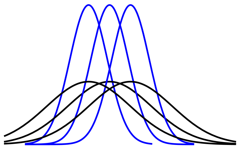
Figure 1: Schematic representation of the distribution of information about the density in the cloud. Black lines: $N$ poorly localized bosons. Blue lines: $N$ ”effective” bosons, better localized for simulation purpose.

We address now how the temporal evolution of the BC-BH system looks like in this framework. The linear dynamics of the BC-BH are implemented and are the evolution rules of the CA. $\bar{N}$ is increased at randomly chosen positions at each timestep in order to simulate superradiance and $\bar{N}_{i,j}(k)$ is the value of the variable at the grid-cell labelled by spatial indices $i$ and $j$, at time step $k$, as explained in detail in Section IV. We record the value of a given parameter $s$ characterizing the system and check if the distribution function of this parameter, $D(s)$, behaves as for a SOC system.

We summarize our assumptions

• There is only one populated energy level. This is equivalent to saying that Eq. (3) expresses, in a linear approximation, the dynamics of the cloud itself. Such an assumption is justified, because the growth rate of the next available energy level is very small compared to $\Gamma_{g}$.

• The dissipation rate $\Gamma_{d}$ is constant as the cloud density grows. By assumption, dissipation is negligible compared to growth, so even if $\Gamma_{d}$ does change, it will not change as much as to affect the dynamics Arvanitaki and Dubovsky (2011).

• The nonlinear and critical limit are the same and occur when the parameter $\epsilon$ reaches its critical value $10^{-4}$, Eq. (4). This is supported by simulations of collapse Kodama and Yoshino (2011).

• the size of the cloud, $L$, is constant and is calculated based on the linear approximation of hydrogenic states.

The mapping between BC-BH and SOC/CA proposed in this paper is summarized in Table 1.

Table 1: Map of BC-BH dynamics to SOC.

SOC/CA framework	BC-BH system
discrete space	2D “cloud”
local interaction	one cloud cell interacts with 3 other cloud cells only at criticality
infinitely slow external drive	bosons are added to the cloud with a very slow rate, $\Gamma_{g}$
SOC occurs as a result of threshold dynamics	when the critical parameter $\epsilon=10^{-4}$ is reached, nonlinearities become important
dissipation	given by the very slow rate $\Gamma_{d}$
observables	distribution of the number of avalanches needed to relax one perturbation

IV Results

We address now the third question posed in the previous Section by formulating the evolution rules for our CA. Let $L$ be the cloud radius, i.e., the $r_{c}$ quantity from Eq. (11) of Arvanitaki and Dubovsky (2011)

$$L\equiv r_{c}=\frac{(n+l+1)^{2}}{(\mu R_{g})^{2}}R_{g},$$ (5)

with $n=0$, $l=1$, $\mu R_{g}=0.42$ and $\mu=3\cdot 10^{-11}eV$. $n$ and $l$ are quantum numbers associated with the hydrogenic state of the cloud and these particular values assure maximum growth. In this case, the constant Gerton et al. (2000) most effective instability rate occurs when Arvanitaki and Dubovsky (2011)

$$\Gamma_{g}=1.5\cdot 10^{-7}rg^{-1}.$$ (6)

The solution of the differential equation (2) is given by

$$N(t)=N_{i}e^{\Gamma_{g}t},$$ (7)

where $N_{i}$ is the initial value of the variable $N$. For simulation purposes, temporal evolution is recorded in discrete timesteps, $\Delta t$. The solution at timestep $k$ may be rewritten as

$$N(k\cdot\Delta t)=N_{i}e^{\Gamma_{g}k\Delta t}.$$ (8)

If $\Delta t$ is taken to be of the order of one gravitational radius and the notation $\bar{\Gamma}_{g}=\Gamma_{g}\Delta t$ is used, the equation for the evolution of the system in natural time units is formally written as

$$N(k)=N_{i}e^{\bar{\Gamma}_{g}k}.$$ (9)

The number of bosons added to the cloud due to superradiance in one natural timestep is given by

$$\Delta N=N(k+1)-N(k)=N_{0}e^{\bar{\Gamma}_{g}k}\left(e^{\bar{\Gamma}_{g}}-1\right).$$ (10)

Since for the QCD axion $e^{k\bar{\Gamma}_{g}}\cong 1$ and $e^{\bar{\Gamma}_{g}}-1\cong 1.5\cdot 10^{-7}$, the dynamics equation used as a basis for the simulation is

$$N(k+1)=N(k)+1.5N_{i}\cdot 10^{-7}.$$ (11)

It is useful to restate this equality in terms of the critical number of bosons, $N_{c}$. We will do this by assuming that the initial number of bosons is some fraction $x\in(0,1)$ of the critical number, $N_{i}=xN_{c}$

$$N(k+1)=N(k)+1.5xN_{c}\cdot 10^{-7}.$$ (12)

$N_{c}$ is easily computable as $N_{c}=M_{BH}\epsilon/\mu=2.4\times 10^{16}$ (all quantities are calculated for mass expressed in eV). So the equation for the temporal evolution of the total number of bosons in the cloud can be written as

$$N(k+1)=N(k)+\Delta N,$$ (13)

where $\Delta N=3.6x\cdot 10^{9}$. This is to be simulated on a $100\times 100$ grid with the help of the parameter $\bar{N}$. One may immediately write

$$\bar{N}_{i,j}(k+1)=\bar{N}_{i,j}(k)+\Delta\bar{N},$$ (14)

for all sites labelled $i,j$ in the grid and at each timestep $k$. This is not general enough because so far we have no reason to believe that the spatial growth of the number of bosons is homogeneous. To circumvent this problem, the same total amount $\Delta N$ will be added to the cloud, but to a limited number of randomly chosen sites, i.e. the update rule for the CA will read

$$\bar{N}_{i,j}(k+1)=\bar{N}_{i,j}(k)+\bar{N}_{0},$$ (15)

for $n$ randomly chosen sites, with $N_{0}=\Delta N/n$. If $n=100$ then $\bar{N}_{0}=3.6x\cdot 10^{7}$. For the discretized case the critical parameter is $\bar{N_{c}}=2.4\cdot 10^{12}$. Dissipation must also be taken into account, but at a much smaller rate. This is modelled as

$$\bar{N}_{i,j}(k+1)=\bar{N}_{i,j}(k)-\bar{N}_{0},$$ (16)

for $m$ randomly chosen sites, with $m\ll n$. For $n=100$ we consider $m=1$. For future reference we note that in numerical simulations the important quantity is actually the ratio $\bar{N}_{c}/\bar{N}_{0}$

$$\frac{\bar{N}_{c}}{\bar{N}_{0}}=6.67\times x^{-1}10^{4}.$$ (17)

To summarize, for a QCD axion with $\mu R_{g}=0.42$, initial cloud population with $x=95\%$ and after rescaling the values of $\bar{N}_{c}$ and $\bar{N}_{0}$ so that $\bar{N}_{0}$ is of order unity (for practical reasons) we get the following parameters used in the simulation

$$\bar{N}_{c}=280000,\mbox{ }\bar{N}_{0}=4$$

$$n=100,\mbox{ }m=1.$$ (18)

In words, at each time step $k$, a number $100$ units are added to the cloud and $\bar{N}$ grows locally. The local enhancement of axion number is done randomly, i.e., $100$ randomly chosen grids will receive one unit. At the same timestep, $1$ unit dissipates from a randomly chosen site and it is assumed that this unit escapes to infinity (it is not fed to the BH). Adding new axions at randomly chosen positions is a nontrivial assumption, but it seems well justified based on two considerations: the observations of laboratory Bosenovas which emphasize the stochastic nature of this process Gerton et al. (2000) and the previous statement that, until the critical limit is reached, the system evolves in a linear regime, Eq. (3).

At each timestep $k$ all the grids are verified to see whether the critical density $\bar{N}_{c}$ is reached. Once the criticality condition is met, the gravitational potential is no longer important and transfer of information is due to the nonlinear interaction of the bosons. The next question is “how many neighbors does the site interact with?” so that information of collapse could be transported to that number of neighbors. We will assume it interacts with 3 sites, namely those three which are nearest neighbors and closer to the BH than the current site. The critical condition and the critical flow are implemented as

$$\mbox{if }\bar{N}_{i,j}(k)>\bar{N}_{c},\mbox{then }$$ (19)

$$\bar{N}_{i,j}(k)\to\bar{N}_{i,j}(k)-3\bar{N}_{0};$$

$$\bar{N}_{i+1,j}(k)\to\bar{N}_{i+1,j}(k)+\bar{N}_{0};$$

$$\bar{N}_{i+1,j-1}(k)\to\bar{N}_{i+1,j-1}(k)+\bar{N}_{0};$$

$$\bar{N}_{i+1,j+1}(k)\to\bar{N}_{i+1,j+1}(k)+\bar{N}_{0};$$

The result of this simulation is the distribution $D(s)$ of event sizes (Fig. 2). This is exactly how an archetypical SOC system behaves Bak et al. (1988) and it is clear that after a growth period Self Organized Criticality is reached and the system stays in this state. This is a first important result.

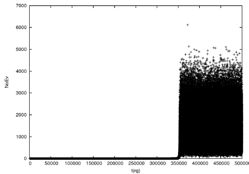
Figure 2: The distribution of event size, $D(s)$ for a QCD-axion cloud in superradiance around a BH. The flow at criticality is given by the rules (19). The cloud was initialized at $95\%$ of its critical boson number $\bar{N}_{c}$.

To test whether or not the fact that the system reaches SOC is rule-dependent, the system evolution is studied for different rules at criticality (different critical flows). The difference is that apart from the three units allowed to move to other sites, an additional number of boson units completely leave the cloud. This was done for $3$ units, $6$ units [Eq. (20), Fig. 3] and $12$ units. For the case of six units, this is written and implemented as

$$\mbox{if }\bar{N}_{i,j}(k)>\bar{N}_{c},\mbox{then }$$ (20)

$$\bar{N}_{i,j}(k)\to\bar{N}_{i,j}(k)-9\bar{N}_{0};$$

$$\bar{N}_{i+1,j}(k)\to\bar{N}_{i+1,j}(k)+\bar{N}_{0};$$

$$\bar{N}_{i+1,j-1}(k)\to\bar{N}_{i+1,j-1}(k)+\bar{N}_{0};$$

$$\bar{N}_{i+1,j+1}(k)\to\bar{N}_{i+1,j+1}(k)+\bar{N}_{0};$$

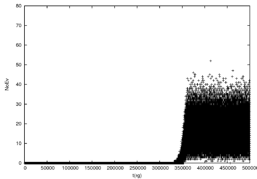
Figure 3: The distribution of event size, $D(s)$ for a QCD-axion cloud in superradiance around a BH. The flow at criticality is given by rules (20). The cloud was initialized at $95\%$ of its critical boson number.

In all cases SOC is reached in a time period that depends on how close $N_{i}$ is to the critical value. The number of events needed to relax the system changes.

A more realistic simulation has to account for when the superradiance condition is no longer fulfilled. It is then we expect that SOC to cease, followed by a transitory period, and afterwards the system will again settle into a SOC state characterized by the new parameters. Due to the limited computational capabilities and the very slow growth rate, we use the fact that the system will eventually be in SOC and initialize the automaton very close to its critical parameter, $x=0.99$.

To compute how much mass the BH has lost because of superradiance, we assume as an example that superradiance stops when $10\%$ of the BH mass is lost, i.e. superradiance stops for $M_{BH}=M$ but immediately starts again for $M_{BH}=0.9M$. All the parameters characteristic to the system, and thus to the simulation, change accordingly. Simulations including the change in superradiance parameters were performed for all 4 sets of rules at criticality. The same qualitative results were obtained in all simulations: there is SOC on both sides of the transition, the transition is sharp and the ratio of the number of events prior to transition and following transition is approximately $2$.

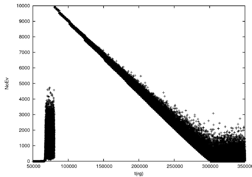
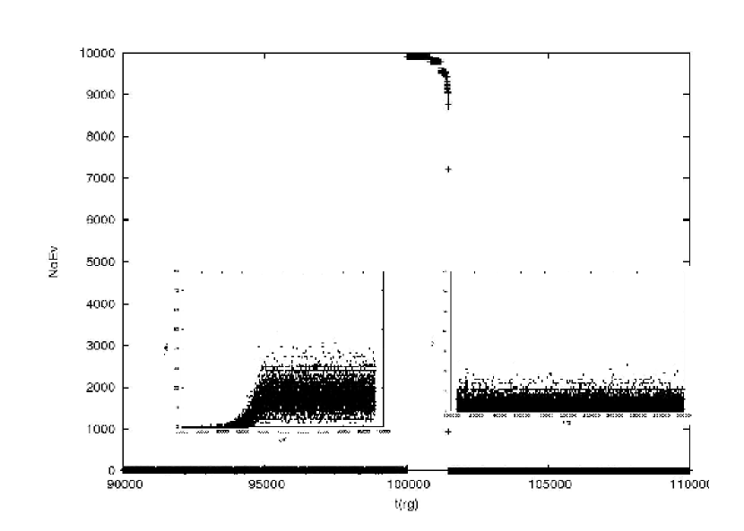
Figure 4: The distribution of event size, $D(s)$ for a QCD-axion cloud in superradiance around a BH. The cloud was initialized at $99\%$ of its critical boson number (the constraint Eq. (17) is obeyed). Transition to another set of superradiance parameters is visible. The flow at criticality is given by rules (19) (upper panel) and for rules (20) (lower panel).

When exiting the superradiance condition for the parameter set governed by $M$, superradiance for the parameter set governed by $=0.9M$ instantly begins according to our rules. The results of this is that $\bar{N}$, which has a value around $\bar{N}_{c}^{M}$ is compared to the lower value of $\bar{N}_{c}^{0.9M}$ and avalanches occur until the new value for the critical parameter is reached and SOC is installed and maintained.

V Summary and open issues

Starting from rigorous analytical results describing the dynamics of a boson-cloud–black-hole (BC-BH) system, we derived a simple map from this dynamics to a cellular automaton. Within our working framework (see assumptions at the end of Section III and Table 1) we have shown that the BC-BH system reaches self-organized criticality (SOC) and stays there as long as the superradiance condition is fulfilled. Since laboratory observations of the growth and collapse of Bose–Einstein condensates lead to a similar picture — albeit only for short timescales, see for instance Fig. 3 in Gerton et al. (2000) — we have some confidence that this is a physical property of our model and not an artifact of inadequate modelling. When the superradiance condition is no longer valid, the evolution rules change quantitatively and the simulated system exhibits a transition after which it again settles into SOC. By varying the rules we checked that this is a rule-independent result (in the sense that it is recovered for all the sets of rules that we have employed) which gives some confidence that this result holds for actual axion cloud near black holes.

The quantitative details of the transition are rule dependent (Figs. 2-4). For the first set of transition rules, Eq. (19), the temporal width of the transition period is quite large, $25\times 10^{4}r_{g}$. For the second set of transition rules, Eq. (20), the temporal width of the transition is of the order $10^{4}r_{g}$. The ratio of the medium numerical value of $D(s)$ before and after transition is approximately $2$ for four different evolutions of the system at criticality. The open issue is whether or not these aspects are related to underlying physics or are numerical artifacts.

We assumed that a new superradiance domain is instantly valid, which led to very large number of events associated with the transition when compared to the SOC state (Fig. 4). An open question is whether or not this assumption is physically justified. This should be investigated in future work.

We expect that observational data of gravitational waves from a large range of masses for BH will be able to shed light on at least two very important issues. One is the physics at transition and observational data will help devise more realistic rules for suitable cellular automata. Also, an appropriate observational database will help in determining the scaling function associated with this phenomena.

Appendix A Sandpile model

SOC may be studied through a simple sand-pile model (Fig. 5) in a CA framework Bak et al. (1988). This arrangement may be thought of as half of a symmetric sand pile with both ends open. The numbers $z_{n}$ characterizing the automaton represent height differences between successive positions along the sand pile, $z_{n}=h(n)-h(n+1)$. When placing a grain of sand in cell $n$ the dynamics of this system follows the rules

$$z_{n} \to z_{n}+1$$ (21)

$$z_{n-1} \to z_{n-1}-1.$$

This model is a cellular automaton where the state of the discrete variable $z_{n}$ at time $t+1$ depends on the state of the variable and its neighbors at time $t$.

When the height difference becomes higher than a threshold (critical) value, $z_{c}$, one unit of sand tumbles to the lower level

$$z_{n} \to z_{n}-2$$ (22)

$$z_{n\pm 1} \to z_{n\pm 1}+1\text{ for }z_{n}>z_{c}.$$

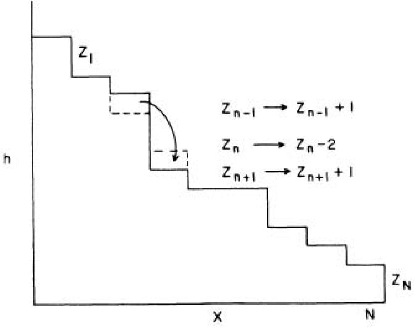
Figure 5: One dimensional sand pile automaton Bak et al. (1988).

The process continues until all the $z_{n}$ are below $z_{c}$. At this point another grain of sand is added at a random site $n$ through Eq. (21).

Starting from a set of initial conditions, the pile grows and in the mean time the slope of the pile increases. It is the value of this slope, as seen in the Eqs. (21), (22), that will at some point reach a critical value. The meaning of the critical value is that if this value is reached and one more grain is added, material will slide. In the critical state the system is just barely stable with respect to further perturbations. Information about the perturbation will be known across all lengthscales in the system.

An event consists of the seed (i.e. placing of the grain) and the subsequent information (grain) transfer or avalanche until complete relaxation. Each event has an associated time $T$ (i.e. the time it takes the perturbation to die out), a cluster size $s$ (i.e. the total number of slidings induced by the perturbation) and a total energy (i.e. release of energy, as transfers occur based on first principles that the final state is an energetically lower state).

For this simple model, the distribution of event sizes $D(s)$ is given by Pruessner (2004)

$$D(s)=\frac{1}{L}\theta\left(L-s\right),$$ (23)

where $L$ is the system size and $\theta(x)$ is the Heaviside step-function. To put this in the form of Eq. (1), we rewrite it as

$$D(s)=\frac{1}{s}\left[\frac{s}{L}\theta\left(1-\frac{s}{L}\right)\right]$$ (24)

and by identification $a=1$, $\tau=1$, $b=1$, $\sigma=1$ and the scaling function is $\mathcal{G}(x)=x\theta\left(1-x\right)$.

References

- Peccei and Quinn (1977) R. Peccei and H. R. Quinn, Phys.Rev.Lett. 38, 1440 (1977).
- Weinberg (1978) S. Weinberg, Phys.Rev.Lett. 40, 223 (1978).
- Wilczek (1978) F. Wilczek, Phys.Rev.Lett. 40, 279 (1978).
- Arvanitaki et al. (2010) A. Arvanitaki, S. Dimopoulos, S. Dubovsky, N. Kaloper, and J. March-Russell, Phys.Rev. D81, 123530 (2010), eprint 0905.4720.
- Arvanitaki and Dubovsky (2011) A. Arvanitaki and S. Dubovsky, Phys.Rev. D83, 044026 (2011), eprint 1004.3558.
- Acharya et al. (2010) B. S. Acharya, K. Bobkov, and P. Kumar, JHEP 1011, 105 (2010), eprint 1004.5138.
- Marsh and Ferreira (2010) D. J. Marsh and P. G. Ferreira, Phys.Rev. D82, 103528 (2010), eprint 1009.3501.
- Panda et al. (2011) S. Panda, Y. Sumitomo, and S. P. Trivedi, Phys.Rev. D83, 083506 (2011), eprint 1011.5877.
- Dubovsky and Gorbenko (2011) S. Dubovsky and V. Gorbenko, Phys.Rev. D83, 106002 (2011), eprint 1012.2893.
- Marsh (2011) D. J. Marsh, Phys.Rev. D83, 123526 (2011), eprint 1102.4851.
- Dubovsky et al. (2011) S. Dubovsky, A. Lawrence, and M. M. Roberts (2011), eprint 1105.3740.
- Kodama and Yoshino (2011) H. Kodama and H. Yoshino (2011), eprint 1108.1365.
- Cardoso et al. (2011) V. Cardoso, S. Chakrabarti, P. Pani, E. Berti, and L. Gualtieri, Phys.Rev.Lett. 107, 241101 (2011), eprint 1109.6021.
- Marsh et al. (2011) D. J. Marsh, E. Macaulay, M. Trebitsch, and P. G. Ferreira (2011), eprint 1110.0502.
- Horbatsch and Burgess (2011) M. Horbatsch and C. Burgess (2011), eprint 1111.4009.
- Alsing et al. (2011) J. Alsing, E. Berti, C. Will, and H. Zaglauer (2011), eprint 1112.4903.
- Amaro-Seoane et al. (2012) P. Amaro-Seoane, S. Aoudia, S. Babak, P. Binetruy, E. Berti, et al. (2012), eprint 1201.3621.
- Penrose (1969) R. Penrose, Riv. Nuovo Cim. 1, 252 (1969).
- Bak et al. (1988) P. Bak, C. Tang, and K. Wiesenfeld, Phys.Rev. A38, 364 (1988).
- Pruessner (2004) G. Pruessner, Ph.D. thesis, Imperial College London (2004).
- Sornette (2000) D. Sornette, Critical phenomena in natural sciences (Springer, 2000).
- Zouros and Eardley (1979) T. Zouros and D. Eardley, Annals Phys. 118, 139 (1979).
- Bandman (2008) O. Bandman, Theory and applications of Cellular Automata, eds. A. Adamatzky, R. Alonso-Sanz, A. Lawniczak, G. Martinez, K. Miorita, T. Worsch pp. 381–397 (2008).
- Gerton et al. (2000) J. Gerton, D. Strekalov, I. Prodan, and R. Hulet, Nature 408, 692 (2000).