Kondo-Anderson transitions

Abstract

Dilute magnetic impurities in a disordered Fermi liquid are considered close to the Anderson metal-insulator transition (AMIT). Critical Power law correlations between electron wave functions at different energies in the vicinity of the AMIT result in the formation of pseudogaps of the local density of states. Magnetic impurities can remain unscreened at such sites. We determine the density of the resulting free magnetic moments in the zero temperature limit. While it is finite on the insulating side of the AMIT, it vanishes at the AMIT, and decays with a power law as function of the distance to the AMIT. Since the fluctuating spins of these free magnetic moments break the time reversal symmetry of the conduction electrons, we find a shift of the AMIT, and the appearance of a semimetal phase. The distribution function of the Kondo temperature $T_{K}$ is derived at the AMIT, in the metallic phase and in the insulator phase. This allows us to find the quantum phase diagram in an external magnetic field $B$ and at finite temperature $T$. We calculate the resulting magnetic susceptibility, the specific heat, and the spin relaxation rate as function of temperature. We find a phase diagram with finite temperature transitions between insulator, critical semimetal, and metal phases. These new types of phase transitions are caused by the interplay between Kondo screening and Anderson localization, with the latter being shifted by the appearance of the temperature-dependent spin-flip scattering rate. Accordingly, we name them Kondo-Anderson transitions (KATs).

I Introduction

The non-Fermi liquid behavior of disordered electronic systems such as the power-law divergence of the low-temperature magnetic susceptibility, can originate from a wide distribution of the Kondo temperatures of magnetic impurities.bhatt ; langenfeld ; dobros ; Miranda The Kondo temperature $T_{K}$ is exponentially dependent on the local exchange coupling $J$ and thus on the hybridization of a magnetic impurity state with the conduction band. Since the hybridization is proportional to the overlap integral between a localized magnetic impurity orbital and the conduction band, it can be exponentially sensitive to microscopic variations of the position of a magnetic impurity.bhatt The exchange coupling also depends on all wave function amplitudes of the conduction electrons at that position, and thus on the local density of states (LDOS) in the conduction band. The distribution of the LDOS depends strongly on the nonmagnetic disorder strength and is known to attain a wide log-normal distribution.lernerldos In the earliest approaches to this problem it was argued that the LDOS in the vicinity of the Fermi energy depends only slowly on energy. Therefore, the small $T_{K}$ tail of the distribution should be directly connected to the distribution of the LDOS at the Fermi energy, which results in a wide distribution of $T_{K}$ on the metallic side of the AMIT whose width increases as the AMIT is approached.dobros However, since $T_{K}$ is determined by an integral over all energies, the fluctuations of the LDOS are to some degree averaged out so that $T_{K}$ may not vary as strongly. In the weak-disorder limit, explicit analytical calculations show that the width of the distribution of Kondo temperatures is finite due to correlations between wave functions at different energies. In disordered metals, these correlations are induced by the diffusion of conduction electrons. However, the resulting width was found to be small in three dimensions in the weak-disorder limit.kettemannjetp ; micklitz For strong disorder the distribution of $T_{K}$ has been studied by means of the exact numerical diagonalization of finite systems to be wide and bimodal.imre ; cornaglia Its low-$T_{K}$ power-law tail has been argued to have a universal power.cornaglia Similar bimodal distributions of $T_{K}$ have been found in 2D disordered metals using the nonperturbative numerical renormalisation group and the quantum Monte Carlo methods.zhuravlev

In this paper, we consider dilute magnetic impurities in a disordered Fermi liquid close to the Anderson metal-insulator transition (AMIT). We use information about the multifractality of the critical wave functions at and in the vicinity of the AMIT, multifractal ; rmpmirlinevers ; rodriguez in order to derive physical properties arising from the interaction between the conduction electron spins and the quantum spins of the magnetic impurities at the transition point. In particular, we obtain analytical expressions for the distribution functions of the Kondo temperature $T_{K}$ at and in the vicinity of the AMIT.

At finite density, the magnetic moments become coupled by the indirect exchange coupling $J^{I}$. dobros The latter can be calculated using the expression for the generalized RKKY coupling,RKKY which is a function of the local exchange coupling $J$.liechtenstein The distribution of $J^{I}$ and its competition with the Kondo screening will be studied in a subsequent article. rkkykondo Here, we consider the dilute limit when the coupling between the moments can still be disregarded. In the metallic phase the density of free, unscreened magnetic moments $n_{FM}$ is found to vanish exactly in the zero-temperature limit. In the insulating phase, $n_{FM}(T=0)$ is finite and increases with a power law as function of the distance to the AMIT.

In Sec. II we begin with a brief review of multifractal statistics. Wave functions in the vicinity of the AMIT are furthermore power-law correlated in energy.powerlaw ; cuevas ; ioffe ; ioffe2 As has been noted in Ref. cuevas, this has the surprising consequence that multifractal eigenfunctions which are close in energy are likely to have their maximal intensity at the same positions in space. This positive correlation has been called stratificationcuevas and is opposite to what is expected in the localized phase where states close in energy have their maximal intensity most likely at far apart positions in space. Another consequence is the opening of local pseudogaps at positions where the critical wave functions have vanishing intensity.kettemann At other sites the local intensity diverges with a power law.

In Sec. III the Kondo problem in disordered systems is formulated.

In Sec. IV the distribution of Kondo temperatures at the AMIT is derived and discussed.

In Sec. V we extend the analysis to the metallic regime where the Fermi energy is located above the mobility edge. Although all states in the vicinity of the Fermi energy are extended, the multifractal nature of the eigenstates on length scales smaller than the correlation length $\xi$ leads to fluctuations of the LDOS and modifies the magnetic properties of the system as we review in Sec. V.

In Sec. VI we extend the analysis to the insulating regime when the Fermi energy is located below the mobility edge and the wave functions are localized exponentially with a localization length $\xi_{c}$. Multifractal fluctuations still occur on length scales smaller than $\xi_{c}$ and the wave functions are power law correlated within a localization volume. It is therefore crucial to take these effects into account in order to get the correct distribution of Kondo temperatures in the insulating phase .

In Sec. VII we summarise the results for the 2D system, where all states are localised.

In Sec. VIII the quantum phase diagram of the Anderson metal-insulator transition in the presence of magnetic impurities is derived and plotted as function of the exchange coupling parameter $J$ and disorder amplitude $W$. We establish the existence of a critical semimetal phase where both the correlation and the localization lengths are infinite within a finite interval of disorder amplitudes, and the conductivity is vanishing.

In Sec. IX we consider how the quantum phase diagram changes in an external magnetic field, which couples via the Zeeman term to the magnetic impurities and via the orbital term to the conduction electrons.

In Sec. X we present the results for the Non-Femi-liquid properties, in particular the magnetic susceptibility, the specific heat, and the spin relaxation rate as functions of temperature, concentration of magnetic moments, and disorder amplitude.

In Sec. XI we study the consequences of the temperature dependence of the spin relaxation rate, which is caused by the Kondo effect. This leads to transitions between insulator, critical semimetal, and metal phases at finite temperatures. These one may call, accordingly, Kondo-Anderson transitions.

In Sec. XII we provide our conclusions, comment on experimental realizations of these transitions, and discuss remaining open problems.

In Appendix A we review the wave function correlations in the vicinity of the AMIT when one state is at the mobility edge. The joint distribution function of eigenfunction intensities is derived such that it matches the critical correlation functions. Next, the correlation function and the joint distribution functions are derived when both eigenstates are located away from the mobility edge of the AMIT. We also discuss and present results on higher moment correlation functions.

In Appendix B we derive the function $F(\alpha,T_{K})$ as defined in Eq. (12).

II Multifractality, Local Pseudogaps and Power Law Divergencies

The AMIT is known to be a 2nd order quantum phase transition, where both the localization length and the correlation length diverge to infinity. At the AMIT the electrons are in a critical state, which is neither extended nor localized, but sparse, as seen in Fig. 1 where the intensity $|\psi_{l}({\bf r})|^{2}$ at the AMIT is plotted.

II.1 Multifractality

This critical state can be characterized by the moments of eigenfunction intensities $|\psi_{l}({\bf r})|^{2}$, which scale as powers of the system linear size $L$,

$$P_{q}=L^{d}\langle\,|\psi_{l}({\bf r})|^{2q}\rangle\sim L^{-\tau_{q}},$$ (1)

where $d$ is the spatial dimension. In a metal the powers $\tau_{q}$ would be given by $d(q-1)$. Critical states are characterized by multifractal dimensions $d_{q}<d$ which may change with the power $q$ of the moments. These are related to the exponents of the q-th moments by $\tau_{q}=d_{q}(q-1)$. The corresponding distribution function of the intensity is close to log-normal in good approximation,rmpmirlinevers

$$P(|\psi_{l}({\bf r})|^{2})=\frac{1}{|\psi_{l}({\bf r})|^{2}}L^{-\frac{(\alpha-\alpha_{0})^{2}}{2\eta}},$$ (2)

where $\alpha=-\ln|\psi_{l}({\bf r})|^{2}/\ln L$, $\eta=2(\alpha_{0}-d)$ and $\alpha_{0}>d$. The multifractal dimension $d_{q}$ is then related to $\alpha_{0}$ by $d_{q}=d-q(\alpha_{0}-d)$ for not too large $q$. At $q_{c}=\alpha_{0}/2/(\alpha_{0}-d)$ there is a termination of $\tau_{q}$ so that it remains constant $\tau_{q}=\tau_{q_{c}}$ for $q>q_{c}$.rmpmirlinevers Throughout this article we assume the validity of this Gaussian distribution of $\alpha$. In Fig. 1 the local intensity is plotted for a critical state at the three-dimensional AMIT as obtained by exact diagonalisation of the Anderson tight binding model with a box distribution of width $W=16.5t$. Here, $t$ is the hopping parameter. The energy is at $E=2t$ on a cubic lattice with spacing $a$, and linear lattice size size $L=100a$. The coloring of the plotted intensity was done according to the amplitude of $\alpha=-\ln|\psi|^{2}/\ln L$. Sites with higher intensity with $\alpha<1.2$ are so rare that their occurrence can not be resolved in this plot. All other sites whose intensities are not plotted correspond to lower intensity with $\alpha>3.0$. Thereby, about 80 $\%$ of the total state intensity is shown in Fig. 1.

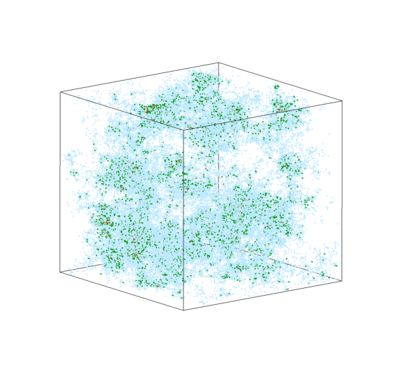
Figure 1: (Color online) The local intensity is plotted here for a critical state at the three-dimensional AMIT, as obtained by exact diagonalisation of the Anderson tight binding model with $W=16.5t$, with hopping parameter $t$ at energy $E=2t$ on a cubic lattice with spacing $a$, and size $L=100a$. The coloring of the plotted intensity was done according to red: $\alpha\in[1.2,1.8]$, green: $\alpha\in[1.8,2.4]$, light blue: $\alpha\in[2.4,3.0]$, where is defined by $\alpha=-\ln|\psi|^{2}/\ln L$. Sites with higher intensity, $\alpha<1.2$, are so rare that their occurrence can not be resolved in this plot. All other sites whose intensities are not plotted correspond to lower intensity $\alpha>3.0$. Thereby, about 80 $\%$ of the total state intensity is shown.

II.2 Critical Correlations

The wave function intensity of a state at energy $E_{l}$ at a certain coordinate ${\bf r}$ has a power-law correlation with the intensity at the mobility edge energy $E_{M}$ with the power $\eta/d$, which is related to $\alpha_{0}$ by

$$\eta=2(\alpha_{0}-d),$$ (3)

(see Eq. (73) in Appendix A).powerlaw ; cuevas As noted in Ref. mirlin, this correlation is due to the fact that eigenstates in the vicinity of the AMIT have a similar multifractal envelope function $\phi_{l}({\bf r})$ and can be written as $\psi_{l}({\bf r})=\phi_{l}({\bf r})\chi_{ul}({\bf r})$. Here $\chi_{ul}({\bf r})$ denotes a factor of the wave function which fluctuates independently from $\phi_{l}({\bf r})$ on short, microscopic length scales.

Joint Distribution Function. One can take this correlation into account by considering the joint distribution function of two wave functions. In order to obtain the correlation function Eq. (73) and the distribution function of a single state, Eq. (2), it should be of the form

$$P(\alpha_{l},\alpha_{k})=\xi_{l}^{a_{lk}\left[f(\alpha_{l})-d\right]}L^{a_{lk}\left[f(\alpha_{k})-d\right]}K_{lk}^{-a_{lk}\frac{(\alpha_{l}-\alpha_{0})(\alpha_{k}-\alpha_{0})}{d\eta}},$$ (4)

where we obtained $K_{{lk}}={\rm Max}\left[|E_{l}-E_{k}|,\Delta_{\xi_{l}}\right]/E_{c}$, see Appendix A for the derivation and definitions of $a_{lk}$. Here, $\xi_{l}$ is the correlation length/ localization length of the state with energy $E_{l}$ on the metallic/insulating side of the transition, and $\Delta_{\xi_{l}}=D/\xi_{l}^{d}$.

Conditional Intensity. Thus, we can derive the conditional intensity of a state at energy $E_{l}$ given that the intensity at the critical energy $E_{k}=E_{M}$ is $|\psi_{M}({\bf r})|^{2}=L^{-\alpha}$. This conditional intensity, relative to the intensity of that of an extended state, is obtained by averaging over the joint distribution function Eq. (4) (for the derivation see Appendix A), kettemann

$$I_{\alpha} = L^{d}\langle|\psi_{l}({\bf r})|^{2}\rangle_{|\psi_{M}({\bf r})|^{2}=L^{-\alpha}}$$ (5)

$$= \left|\frac{E_{l}-E_{M}}{E_{c}}\right|^{r_{\alpha}},$$

where the power is given by

$$r_{\alpha}=\frac{\alpha-\alpha_{0}}{d}-\frac{\eta}{2d}g_{lM}.$$ (6)

This result is valid for $|E_{l}-E_{M}|<E_{c}$, where $E_{c}$ is the energy scale over which the critical correlations exist and $g_{lM}=\ln|(E_{l}-E_{M})/E_{c}|/(d\ln L)$. The average is done over the intensity $|\psi_{l}({\bf r})|^{2}$ using the conditional distribution function, Eq. (81). fixing the intensity $L^{-\alpha}$ at the AMIT. Typically, $E_{c}$ is a fraction of the bandwidth $D$: $E_{c}\sim D/(2d\ln 2d)$.powerlaw When $E_{l}$ is located at a finite energy interval away from the mobility edge $E_{M}$, the coefficient $g_{lM}=\ln|(E_{l}-E_{M})/E_{c}|/(d\ln L)$ vanishes for $L\rightarrow\infty$. Close to $E_{M}$ the coefficient saturates: $g_{lM}|_{E_{l}\rightarrow E_{M}}\rightarrow-1$ and Eq. (5) reduces to $L^{d-\alpha}$, the local intensity at $E_{M}$ relative to the intensity of an extended state $L^{-d}$. Note that in Eq. (5) the average over the uncorrelated factor of the wave function $\chi_{ul}({\bf r})$ has been done, which is $\langle|\chi_{ul}({\bf r})|^{2}\rangle=1$.

Local Pseudogaps. From Eq. (5) we see that at positions in space where the local wave function intensity at the mobility edge is small, corresponding to $\alpha$ larger than its typical value $\alpha_{0}$, the wave function intensity is suppressed within an energy range of order $E_{c}$ around $E_{M}$. Thereby local pseudogaps are formed with a power $r_{\alpha}=\frac{\alpha-\alpha_{0}}{d}$ with vanishing LDOS at the mobility edge, as shown in Fig. 2.

Local Power Law Divergency. On the other hand, when the intensity at the mobility edge is larger than its typical value $L^{-\alpha_{0}}$, which corresponds to $\alpha<\alpha_{0}$, the LDOS is enhanced within an energy range of order $E_{c}$ around $E_{M}$, increasing as a power law when $E_{l}$ approaches the mobility edge, as shown in Fig. 2.

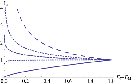
Figure 2: (Color online) The conditional intensity $I_{\alpha}$ relative to the intensity of an extended state as function of the distance in energy to the mobility edge in units of the correlation energy $E_{c}$. The exponent $\alpha$, which is related to the intensity $L^{-\alpha}$ at $E_{M}$, takes the values $\alpha=2,3,3.5,4,6$ in the sequence of decreasing dashing. Local pseudo gaps are seen for $\alpha>\alpha_{0}$, while local power law divergences occur for $\alpha<\alpha_{0}$. Here, we set $d=3$ and $\alpha_{0}=4$.

III Kondo Effect in a Disordered Electron System

III.1 Kondo Impurity Hamiltonian

Magnetic impurities are generally described by an Anderson model where a localized level with energy $\epsilon_{d}$ and on-site Coulomb repulsion $U$ hybridizes with electrons in the conduction band which is described by a Hamiltonian $H_{0}$.andersonmm This Hamiltonian may include the random potential of nonmagnetic impurities $V({\bf r})$. Using the eigenstates $\{\psi_{n}\}$ and energies $\{E_{n}\}$ of $H_{0}$, with the corresponding one-particle density operator given by $\hat{n}_{n,\sigma}$, the Anderson Hamiltonian is written as

$$H_{A} = \sum_{n,\sigma}E_{n}\,\hat{n}_{n,\sigma}+\epsilon_{d}\sum_{\sigma}\hat{n}_{d,\sigma}+U\,\hat{n}_{d,+}\hat{n}_{d,-}$$ (7)

$$+\ \sum_{n,\sigma}\left(t_{nd}\,c_{n\sigma}^{+}d_{\sigma}+\mbox{H.c.}\right),$$

where $\hat{n}_{d,\sigma}$ is the density operator of the impurity level. The hybridization amplitude $t_{nd}$ is proportional to the eigenfunction amplitude at the position of the magnetic impurity $\psi_{n}^{\ast}(0)$ and to the localized orbital amplitude $\phi_{d}(0)$: $t_{nd}=t\,\psi_{n}^{*}(0)\phi_{d}(0)$. One can employ the Schrieffer-Wolff transformation,hewson ; pseudogap formulated in terms of eigenstates $\psi_{n}$ to take into account double occupancy up to second order in $t_{nd}$.kettemannjetp The result is an s-d contact Hamiltonian with exchange couplings given by

$$J_{nn^{\prime}}=t_{nd}^{\ast}\,t_{n^{\prime}d}\left(\frac{1}{U+\epsilon_{d}-E_{n^{\prime}}}+\frac{1}{E_{n}-\epsilon_{d}}\right)$$ (8)

and an additional potential scattering term with amplitude

$$K_{nn^{\prime}}=t_{nd}^{\ast}\,t_{n^{\prime}d}\left(-\frac{1}{U+\epsilon_{d}-E_{n^{\prime}}}+\frac{1}{E_{n}-\epsilon_{d}}\right).$$ (9)

Note that in the symmetric Anderson model, $K_{nn^{\prime}}$ vanishes for all $n,n^{\prime}$ when $|E_{n,n^{\prime}}-E_{F}|\ll U$, since, in this case $\epsilon_{d}=E_{F}-U/2$, where $E_{F}$ is the Fermi energy. For arbitrary $\epsilon_{d}$ wave functions with small amplitude at the position of the magnetic impurity are hardly modified by this potential scattering term since $K_{nn^{\prime}}\sim\psi_{n}^{*}(0)\psi_{n^{\prime}}(0)$. Hence, we will first retain only the exchange couplings $J_{nn^{\prime}}=J\psi_{n}^{\ast}(0)\psi_{n^{\prime}}(0)$, with $J\sim t^{2}/U$, and leave the discussion of possible effects of finite $K_{n,n^{\prime}}$ to Sec. XII.

III.2 Kondo Temperature

As we have shown previously with the numerical renormalization group and the quantum Monte Carlo methods,zhuravlev the distribution of Kondo temperatures is in very good qualitative agreement with the one obtained from the one-loop equation of Nagaoka and Suhl.suhl Only, its average needs to be rescaled, in order to account for a shift of the distribution towards larger values of $T_{K}$ due to the higher-loop corrections.zu96 ; zhuravlev Therefore, we will use here the one-loop equation to calculate $T_{K}$, as given by

$$1=j\frac{\Delta}{2}\sum_{l}\frac{L^{d}|\psi_{l}({\bf r})|^{2}}{\epsilon_{l}}\tanh\left(\frac{\epsilon_{l}}{2T_{K}}\right)\equiv F(\{\alpha_{l}\},T_{K}),$$ (10)

where $j=J/D$, $\Delta=D/N$ is the mean level spacing and $\epsilon_{l}=E_{l}-E_{n}$. $N$ is the number of states in the sample of volume $V=L^{d}$. This defines the Kondo-temperature in terms of the local intensities at all energies $\epsilon_{l}$ in the sample.

III.3 Distribution Function of the Kondo temperature

Thus, one can derive the distribution function of $T_{K}$, when the distribution function of all intensities $P(\alpha_{1},...,\alpha_{l},...,\alpha_{N})$ is known, by solving

$$P(T_{K})=\int\prod_{l}d\alpha_{l}P(\{\alpha_{l}\})\delta(1-F(\{\alpha_{l}\},T_{K}))|\frac{dF}{dT_{K}}|,$$ (11)

where $F(\{\alpha_{l}\},T_{K})$ is defined by Eq. (10). Note that $F(\{\alpha_{l}\},T_{K})$ is always a decreasing function of $T_{K}$, so that $|\frac{dF}{dT_{K}}|=-\frac{dF}{dT_{K}}$.

IV Kondo Effect at the Anderson-Metal-Insulator Transition

Conditional Average. In a first attempt to get its distribution function we calculate the Kondo temperature $T_{K}$ for a given intensity $\xi^{-\alpha}$ at the Fermi energy, and integrate over all other intensities with the conditional distribution function Eq. (81) for fixed $\alpha$. Thereby we find $T_{K}(\alpha)$ as a function of $\alpha$, using that the conditional intensity of state $l$, $\langle|\psi_{l}({\bf r})|^{2}\rangle_{|\psi_{n}({\bf r})|^{2}=L^{-\alpha}}$ is given by Eq. (5),

$$1=j\frac{\Delta}{E_{c}}\sum_{\epsilon_{l}<E_{c}}\left|\frac{\epsilon_{l}}{E_{c}}\right|^{r_{\alpha}-1}\tanh\left(\frac{\epsilon_{l}}{2T_{K}}\right)\equiv F[\alpha,T_{K}],$$ (12)

where the summation over $l$ is restricted to energies within the energy interval of the correlation Energy $E_{c}$ around the mobility edge.remark

We note that Eq. (12) defines the Kondo temperature in a system with pseudogaps of power $r_{\alpha}$, Eq. (6), in the local density of states shown in Fig. 2, when this power is positive.pseudogap Therefore, the Kondo temperature is reduced at such sites, since the magnetic impurities are placed in the locally suppressed LDOS of the conduction electrons.

On the other hand, at sites where the power $r_{\alpha}$ is negative the opposite occurs and $T_{K}$ is enhanced. The Kondo problem with a power-law divergence in the density of states was studied in Ref. bulla, , finding an enhancement of $T_{K}$ towards the strong coupling fixed point given by $J$. Since $\alpha$ is distributed over all values from $0$ to infinity according to Eq. (2), we find by solving Eq. (12) that $T_{K}(\alpha)$ is distributed, accordingly. We note that Eq. (10) is averaged over the uncorrelated part of the wave function, $\chi_{ul}({\bf r})$. Since these short scale fluctuations are uncorrelated in energy, they are averaged out by the summation over energy levels $l$ in Eq. (12), and gives rise to small fluctuations of $T_{K}$ of order of $1/N$, only. Therefore their effect on the distribution of $T_{K}$ is negligible in the thermodynamic limit.

We can now proceed and solve Eq. (12) analytically in various limits. The Kondo temperature for a given intensity $|\psi_{n}({\bf r})|^{2}=L^{-\alpha}$ at the Fermi energy is for $\alpha>\alpha_{0}-d$ found to be given by

$$\frac{T_{K}}{E_{c}}=\left[\left(1-\frac{\alpha-\alpha_{0}}{d}\frac{1}{j}\right)c_{\alpha}\right]^{\frac{d}{\alpha-\alpha_{0}}}.$$ (13)

Here, $j=J/D$ and $c_{\alpha}=\frac{2\alpha-\eta}{\alpha-\eta/2+d}$. Eq. (13) takes into account the critical correlations at the AMIT. In deriving it (see Appendix B for details), we approximate $\tanh x\approx x$ for $x<1$, and $\tanh x\approx 1$ for $x>1$, yielding two terms. One includes the integral over all energies within a window of width $2T_{K}$ around the Fermi energy. The other one is over all larger energies in the conduction bands. In order that the resulting equation is valid for all $\alpha$ it is important to keep both terms.

For the typical value $\alpha=\alpha_{0}$ we recover $T_{K}$ of a clean system in the one-loop approximation, namely,

$$T_{K}(\alpha=\alpha_{0})\sim E_{c}\exp(-1/j)\sim T_{K}^{(0)}.$$ (14)

From Eq. (13) we see that at particular sites where the wave function amplitude is large, corresponding to $\alpha<\alpha_{0}$, $T_{K}$ becomes enhanced. In particular, for a wave function intensity comparable to the one of a metallic state, $\alpha=d$, we find that

$$T_{K}(\alpha=d)\sim j^{2/\eta/d}.$$ (15)

This is larger than $T_{K}^{(0)}$ when $j<1$.

IV.1 Density of Free Magnetic Moments at Zero Temperature.

At sites where the wave function amplitude is small, corresponding to $\alpha>\alpha_{0}$, $T_{K}$ is suppressed due to the appearance of local pseudogaps. The Kondo temperature in the presence of pseudogaps of power $r$ is well known to vanish when the exchange coupling does not exceed a critical value $j_{c}=r$.pseudogap Since the power of the local pseudogaps depend on $\alpha$, Eq. (6), that critical value $j_{c}(\alpha)$ depends on $\alpha$ as well. Accordingly, magnetic moments remain unscreened even at $T=0K$, when $\alpha$ exceeds the critical value

$$\alpha_{\rm FM}=\alpha_{0}+dj.$$ (16)

Out of the $N=L^{d}$ atomic sites in the system, magnetic moments remain free at all temperatures if placed on one of $N_{FM}$ sites, where a sufficiently strong local pseudo gap is developed. Thus, for small $J$ there can be a macroscopic number of such sites, although their density $n_{\rm FM}=N_{\rm FM}/N$,

$$n_{\rm FM}(T=0K)=L^{-d^{2}\frac{j^{2}}{2\eta}}n_{\rm M},$$ (17)

vanishes, $n_{\rm FM}\rightarrow 0$ for $L\rightarrow\infty$.

IV.2 Distribution Function of Kondo Temperature.

IV.2.1 $T_{K}\rightarrow 0$ Limit of $P(T_{K})$

In deriving the conditional intensity, Eq. (5), and inserting it in Eq. (12) we took into account the correlations of all states to the intensity at the Fermi energy as characterised by local pseudogaps and power law divergencies. Since their power $r_{\alpha}$ is distributed, we can now obtain the distribution of the Kondo temperature $T_{K}$ by solving Eq. (13) for $\alpha(T_{K})$ and inserting it in $P(\alpha)$. To this end, we use the Fourier representation of the delta-function. Then, we can expand in $F[\{\alpha_{l}\},T_{K}]$ and perform the average, keeping $\alpha_{l}=\alpha$ at the Fermi energy $E_{F}=E_{M}$ fixed. Next, we use the conditional pair approximation introduced above. If we impose the condition $F[\{\alpha_{l}\},T_{K}]=1$ to obtain $T_{K}$ for given $\alpha$ and insert this in $P(\alpha(T_{K}))$ this yields in the limit of small $T_{K}\rightarrow\Delta$,

$$P^{0}(T_{K}\rightarrow 0)\sim\left(\frac{T_{K}}{E_{c}}\right)^{j-1}L^{-\frac{(dj)^{2}}{2\eta}}.$$ (18)

For $j=0.25$ the power of the $T_{K}\rightarrow 0$ tail is $\beta=1-j=0.75$ in exact agreement with the numerical result in 3 dimensions reported in Ref. cornaglia, . However, we find that its weight is vanishing with a power of the system size $L$. Note that the number of sites used in Ref. cornaglia, is $N=2197$, yielding a level spacing $\Delta/T^{0}_{K}\approx 0.025$, so that Eq. (18) indeed can explain the tail of the distribution $T_{K}\leq\Delta$ displayed in their Fig. 3. Clearly, at larger $T_{K}$ the fluctuations of the wave function intensities at energies away from the AMIT are important. These can strongly change $T_{K}$ and the width of its distribution as we find in the next subsection.

IV.2.2 $P(T_{K})$ for $T_{K}>\Delta$

In order to proceed in the calculation of $P(T_{K})$, at $T_{K}$ exceeding the level spacing $\Delta$ we need to take into account the fluctuations of the intensities at all energies. To this end, let us first rewrite Eq. (11) as

$$P(T_{K})=-\int_{0}^{\infty}d\alpha P(\alpha)\langle\frac{dF}{dT_{K}}\delta(1-F)\rangle_{\alpha},$$ (19)

where $\langle...\rangle_{{\alpha}}$ denotes the average over all intensities, except the one at the Fermi energy which is fixed to $L^{-\alpha}$. Next, we use the Fourier representation of the delta-function to get

$$P(T_{K})=-\int_{0}^{\infty}d\alpha P(\alpha)\frac{d}{dT_{K}}\int_{-\infty}^{\infty}dt\frac{ie^{it}}{2\pi t}$$

$$\times\langle\exp\left(-itF[T_{K}]\right)\rangle_{\alpha}.$$ (20)

Now we can expand $F[\{\alpha_{l}\},T_{K}]$, around $F[\alpha,T_{K}]=\langle F\rangle_{\alpha}$ to take into account the fluctuations of all intensities. Expanding in $\delta F=F[\{\alpha_{l}\},T_{K}]-F[\alpha,T_{K}]$, and performing the integral over $t$, we find

$$P(T_{K})=-\int_{0}^{\infty}\frac{d\alpha}{\sqrt{2\pi}\Gamma}P(\alpha)\frac{dF[\alpha,T_{K}]}{dT_{K}}e^{-\frac{(1-F[\alpha,T_{K}])^{2}}{2\Gamma^{2}}},$$ (21)

where $F[\alpha,T_{K}]=\langle F\rangle_{\alpha}$, is given by Eq. (88) and $\Gamma$ is defined by

$$\Gamma^{2}=\langle F^{2}\rangle_{\alpha}-\langle F\rangle_{\alpha}^{2},$$ (22)

where $\langle...\rangle_{\alpha}$ denotes the average over all $\alpha_{l}$, keeping only $\alpha$ at the Fermi energy fixed. We find, that for $\Delta\leq T_{K}\ll E_{c}$,

$$\Gamma^{2} \approx j^{2}\frac{(T_{K}-\Delta)^{2}}{T_{K}^{2}}\left(c_{1}(\frac{T_{K}-\Delta}{E_{c}})^{-\eta/d}-c_{2}\right.$$ (23)

$$\left.+5\ln[\frac{T_{K}}{E_{c}}]-2\ln[\frac{T_{K}}{E_{c}}]^{2}\right),$$

where we determined numerically, $c_{1}\approx 7.51$ and $c_{2}\approx 9.60$. Note that $\Gamma$ vanishes in the limit $T_{K}\rightarrow\Delta$, $\Gamma(T_{K}\rightarrow\Delta)=0$, since then only energy levels in a range of order $\Delta$ around the Fermi energy contribute, whose correlations are taken into account correctly by $F_{\alpha}$, already. Thus in this limit, the condition $1=F(\alpha,T_{K})$ is imposed exactly, and we recover the tail of the distribution, Eq. (18), diverging with the power $\beta=1-j$.

At larger $T_{K}>\Delta$, $\Gamma$ has a finite value and decays for $\Delta<T_{K}\ll E_{c}$ with the power $\eta/d$. $P(\alpha)$ is peaked at $\alpha=\alpha_{0}$ with a width that scales with the system size as $1/\sqrt{\ln L}$. Thus, for $L\rightarrow\infty$, $\alpha=\alpha_{0}$ is imposed in Eq. (21) for any finite $T_{K}$. Thus we can substitute

$$\langle F[T_{K}]\rangle=j(\frac{T_{K}-\Delta}{2T_{K}}+\ln\frac{D}{2{\rm Max}(T_{K},\Delta)}),$$ (24)

and find that the distribution diverges at $\Delta<T_{K}\ll T_{K}^{(0)}$ as

$$P(T_{K}) \approx\left(\frac{T_{K}}{E_{c}}\right)^{\frac{\eta}{2d}-1}\times$$ (25)

$$\exp\left\{-\frac{1}{2c_{1}}\left(\frac{T_{K}}{E_{c}}\right)^{\eta/d}\ln^{2}\left[\frac{T_{K}}{T_{K}^{(0)}}\right]\right\}.$$

with the power $\beta=1-\eta/d/2$. In $d=3$ dimensions, with $\alpha_{0}=4$, the power is $\beta_{d=3}=2/3$ which is smaller than the one obtained numerically in Ref. cornaglia, , $\beta\approx 0.75$. We note, that there is a noticeable deviation towards smaller powers for $T_{K}>\Delta\approx 0.03$ in the Fig. 3 of Ref. cornaglia, .

V Kondo Effect in the Metal Phase

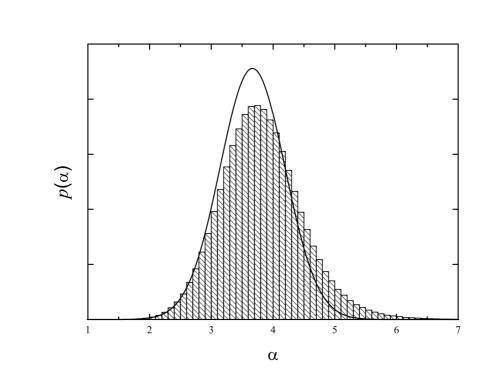
Figure 3: The distribution of $\alpha$ defined in the metallic regime by Eq. (26), as obtained by exact numerical diagonalisation of a 3D sample of size $L^{3}=128^{3}$ in units of the grid cell volume $a^{3}$. The energy of that state is approximately $E=0$, and a box distribution of uncorrelated disorder potential with $W=15t$ is taken. The analytical expression Eq. (27) is plotted for comparison as the solid line for a correlation length $\xi=22a$ (taken from the numerical results of Ref. kmkprl, ).

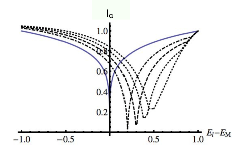
Figure 4: (Color online) The conditional intensity $I_{\alpha}$ at energy $E_{l}$, given that a state at the energy $E_{k}$ has intensity $L^{d}|\psi_{k}({\bf r})|^{2}=\xi_{k}^{d-\alpha}$, relative to the intensity of an extended state. It is plotted as function of the distance of energy $E_{l}$ from the mobility edge energy $E_{M}$, in units of the correlation energy $E_{c}$. The exponent $\alpha$ at the energy $E_{k}$, takes the value $\alpha=4.5$. The energy $E_{k}$ is varied from the mobility edge into the metallic regime with $(E_{k}-E_{M})/E_{c}=0,0.2,0.3,0.4,0.7$, from left to right. Instead of a local pseudo gap, one sees an increasingly shallow depression. Here we set $d=3$ and $\alpha_{0}=4$. Note that it varies slowly in a range $\Delta_{\xi_{k}}$ around the Fermi energy.

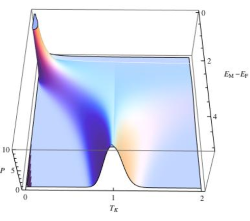
Figure 5: (Color online) The distribution of Kondo temperatures $T_{K}$ in units of $T_{K}^{(0)}$ in the metallic phase, Eq. (33), is plotted as function of the distance to the mobility edge, $E_{F}-E_{M}$ in units of $E_{c}$ for an exchange coupling $j=1/5$.

V.1 Multifractality in the Metallic Phase

In the metallic regime all wave functions are extended and their intensities scale with the inverse system volume, $|\psi|^{2}\sim L^{-d}$. On length scales smaller than the correlation length $\xi$, multifractal fluctuations of the wave function intensity occur as long as $\xi$ is larger than the microscopic length scale $a_{c}$.cuevas ; ioffe2 As pointed out in Refs. ioffe2, ; mirlin, the moments of the intensity do scale with the correlation length $\xi$ as $L^{dq}\langle|\psi|^{2q}\rangle\sim\xi^{(d-d_{q})(q-1)}$. Therefore, in the metallic regime we define $\alpha$ as

$$L^{d}|\psi_{l}({\bf r})|^{2}=\xi_{l}^{d-\alpha_{l}},$$ (26)

where $\xi_{l}$ is the correlation length of state $l$. Notice that this definition of $\alpha$ crosses over to the one we used above in the critical regime, where $\xi$ diverges and is replaced by the system size $L$, when $L<\xi$. It has to a good approximation still the Gaussian distribution,

$$P(\alpha_{l})\sim\exp[-\ln\xi_{l}\frac{(\alpha_{l}-\alpha_{0})^{2}}{2\eta}],$$ (27)

where its width scales with the logarithm of the correlation length $\xi_{l}$. This is confirmed in Fig. 3, where we plot Eq. (27) together with the numerical result, as obtained from exact diagonalisation.

V.2 Intensity Correlations in the Metal

There are still power-law correlations in energy between wave function intensities as given by Eq. (77). Averaging with the conditional distribution function Eq. (78) in the metallic regime, we find the conditional intensity in the metallic regime: given that a state at the energy $E_{k}$ has intensity $L^{d}|\psi_{k}({\bf r})|^{2}=\xi_{k}^{d-\alpha}$, a state at energy $E_{l}$ at position ${\bf r}$ has on average the intensity

$$I_{\alpha{\rm}}(\xi_{l},\xi_{k})=\langle L^{d}|\psi_{l}({\bf r})|^{2}\rangle_{\alpha}=K_{lk}^{\frac{\alpha-\alpha_{0}}{d}-\frac{\eta}{2d^{2}}\frac{\ln K_{lk}}{\ln\xi_{k}}},$$ (28)

where $K_{{lk}}={\rm Max}\left\{|E_{l}-E_{k}|,{\rm Min}(\Delta_{\xi_{l}},\Delta_{\xi_{k}})\right\}/E_{c}$ and

$$\Delta_{\xi_{l}}=E_{c}(a_{c}/\xi_{l})^{d},$$ (29)

is the mean level spacing of a sample of finite size $\xi_{l}$ (for the derivation, see Appendix A). Thus, the intensity at the energy $E_{l}$ has still a dip when $\alpha>\alpha_{0}$, although the LDOS at energy $E_{l}\rightarrow E_{k}$ is no longer suppressed to zero but rather to a finite value (see Fig. 4), given by,

$$\langle L^{d}|\psi_{l}({\bf r})|^{2}\rangle_{\alpha}|_{E_{l}\rightarrow E_{k}}=\xi_{k}^{(d-\alpha)}=\left|\frac{E_{k}-E_{M}}{E_{c}}\right|^{\nu(\alpha-d)},$$ (30)

which is slowly varying with energy in an interval of order $\Delta_{\xi_{k}}$ around the Fermi energy.

V.3 Distribution of Kondo Temperatures

Since the intensity is finite at all sites in the metallic regime we expect that the magnetic impurity spin is at low temperatures always screened. Therefore, the Kondo temperature does not vanish in the metallic regime at any site. According to Eq. (30) the local intensity can be substantially suppressed or enhanced, depending on the random value of $\alpha$. Its distribution, as given by Eq. (27), has a finite width. On the other hand, the second moment of $F$ does saturate to a finite value when $T_{K}<\Delta_{\xi}$:

$$\Gamma^{2}|_{T_{K}<\Delta_{\xi}}\rightarrow j^{2}c_{1}(\frac{\Delta_{\xi}}{E_{c}})^{-\eta/d},$$ (31)

where $c_{1}\approx 7.51$. Inserting both Eqs. (31,27) into the expression for $P(T_{K})$, Eq. (21) we find that the probability to find a small Kondo temperature such that $T_{K}<\Delta_{\xi}=|(E_{F}-E_{M})/E_{c}|^{\nu d}$, is decaying to zero as

$$P(T_{K}) \approx\left(\frac{\Delta_{\xi}}{E_{c}}\right)^{\frac{\eta}{2d}}\frac{1}{T_{K}}e^{-\frac{1}{2c_{1}}\left(\frac{\Delta_{\xi}}{E_{c}}\right)^{\eta/d}\ln^{2}\left(\frac{T_{K}}{T_{K}^{(0)}}\right)}.$$ (32)

Thus, in the metallic phase $E_{F}>E_{M}$ there are no free magnetic moments and the low $T_{K}$-tail terminates at $T_{K}\approx\Delta_{\xi}$ as seen in Fig. (5). For $T_{K}>\Delta_{\xi}$ a power law tail of the distribution can still be observed, as seen in Fig. (5). There, we plot $P(T_{K})$ as obtained by Eq. (25) and substituting $T_{K}$ by ${\rm Max}(T_{K},\Delta_{\xi})$ in the expression for $\Gamma$, Eq. (23),

$$P(T_{K}) \approx\left(\frac{Max(T_{K},\Delta_{\xi})}{E_{c}}\right)^{\frac{\eta}{2d}}\frac{1}{T_{K}}\times$$ (33)

$$\exp\left\{-\frac{1}{2c_{1}}\left(\frac{Max(T_{K},\Delta_{\xi})}{E_{c}}\right)^{\eta/d}\ln^{2}\left[\frac{T_{K}}{T_{K}^{(0)}}\right]\right\}.$$

VI Kondo Effect in the Insulator

In the insulating regime each localized state is restricted to a volume of the order of $\xi_{l}^{d}=\xi_{c}^{d}(E_{l})$, the localization volume. On length scales smaller than the localization length $\xi_{l}$ there are still multifractal fluctuations. In addition, the wave functions in the insulating regime are power-law correlated close to the AMIT.cuevas Neglecting a small logarithmic enhancement which occurs at energy spacings smaller than the local level spacing $\Delta_{\xi}=\xi^{-d}D$,cuevas we can get the distribution of $T_{K}$ simply by using the results obtained at the critical point and replacing the system size $L$ by the localization length $\xi_{c}$. Defining

$$|\psi_{l}(x)|^{2}=\xi_{l}^{-\alpha},$$ (34)

we thus find that the distribution function of $\alpha$ within a localization volume is the same as if we had considered the distribution at the AMIT in a finite volume of order $\xi_{l}^{d}$. We note that the probability to find a state at energy $E_{l}$ inside the localization volume is decaying with the system volume $L^{d}$ as $\xi_{l}^{d}/L^{d}$. Outside the localization volume the intensity decays exponentially, $|\psi_{l}({\bf r})|^{2}\sim\exp[-2r/\xi]$ corresponding to $\alpha=2r/(\xi_{l}\ln\xi_{l})$. Since most sites in the sample are a distance $r\sim L\rightarrow\infty$ away from the localization volume one finds $\alpha\sim L\rightarrow\infty$ at most sites of the sample. The correlation function between two wave functions at different energies $E_{l}$ and $E_{k}$ is still given by Eq. (73) where $\Delta_{\xi_{l}}$ is now the local level spacing at energy $E_{l}$. Accordingly, the joint distribution function has the form given in Eq. (78). However, the difference to the metallic regime is that there are only discrete energy levels which are separated by the local level spacing $\Delta_{\xi_{l}}$. This difference is important, especially when calculating the Kondo temperature, since the hard gap $\Delta_{\xi_{l}}$ in the insulating regime cuts off the Kondo renormalization flow at small energies.meraikh

Thus, we can conclude that there is a finite density of free magnetic moments $n_{FM}$, which remain unscreened. Therefore, we need to subtract this density from the distribution function of $T_{K}$ given by Eq. (21). The width $\Gamma$ is given by Eq. (23) when substituting $\Delta$ by the level spacing in a localization volume, $\Delta_{\xi}$ for $T_{K}\geq\Delta_{\xi}$,

$$\Gamma^{2} \approx j^{2}\frac{(T_{K}-\Delta_{\xi})^{2}}{T_{K}^{2}}c_{1}(\frac{T_{K}-\Delta_{\xi}}{E_{c}})^{-\eta/d},$$ (35)

where $c_{1}\approx 7.51$. For $T_{K}<\Delta_{\xi}$, we find that it vanishes, $\Gamma=0$, and the condition $1-F_{\alpha}$ is enforced exactly. Therefore, we get from Eq. (21) the low $T_{K}$ tail in the localised regime as

$$P(T_{K})=\left(1-\frac{n_{FM}(T=0)}{n_{M}}\right)\left(\frac{E_{c}}{T_{K}}\right)^{1-j}\xi^{-\frac{1}{2\eta}(dj)^{2}}.$$ (36)

Thus, we find that the distribution diverges with the power $\beta=1-j$. This is in full agreement with the numerical results of Ref. cornaglia, , where a power $0.75$ has been obtained for $j=0.25$ for a wide range of disorder amplitude $W$. Also, the increase of the weight of the power law tail with disorder strength $W$ is in good agreement with the numerical results.

The finite density of free magnetic moments is found to be,kettemann

$$n_{\rm FM}(T=0K) = n_{M}\xi^{-\frac{1}{2\eta}(dj)^{2}}$$ (37)

$$= n_{M}\left(\frac{W-W_{c}}{W_{c}}\right)^{\frac{\nu}{2\eta}(dj)^{2}},$$

which decays to zero as a power law when the disorder amplitude $W$ approaches the AMIT at $W_{c}$. It converges to the total density of magnetic moments $n_{M}$ far away from the mobility edge, $E_{M}-E_{F}\rightarrow E_{c}$. Thus, according to this expression all magnetic moments should be free in the strongly localized regime where $\xi\rightarrow a_{c}$.

VII Kondo Effect in 2D Anderson Insulators

We can apply this analysis also to two-dimensional disordered electron systems, where all states are localized. The Kondo effect in such systems has been studied numerically based on the 1-loop equation,kettemannjetp ; cornaglia and with nonperturbative methods in Ref. zhuravlev, , where both the distribution of Kondo temperatures and the density of free magnetic moments have been obtained. The two-dimensional localization length in the absence of a magnetic field is known to depend exponentially on the disorder strength, $\xi_{2D}=g\exp(\pi g)$, where $g=E_{F}\tau$. The scattering rate $1/\tau$ is related to the disorder amplitude $W$ as $1/\tau=\pi W^{2}/6D$. There are weak wave function correlations in two dimensions which are logarithmic, with an amplitude of order $1/g$. For weak disorder, $g\gg 1$ we can rewrite this correlation as an effective power law with power

$$\eta_{2D}=2/\pi g.$$ (38)

The correlation energy in 2D is of the order of the elastic scattering rate, $E_{c~{}2D}\sim 1/\tau$. Thus, for systems whose size $L$ is smaller than the localization length $\xi_{{2D}}$, the 2D system behaves like a critical system with $\alpha_{0}$ defined by $\eta_{2D}=2/\pi g=\alpha_{0}-2$, or

$$\alpha_{0}=2+\frac{2}{\pi g}.$$ (39)

There is a critical exchange coupling $J_{c}^{(1)}$ above which there is no more than one free magnetic moment in the whole sample.kettemann Substituting $\eta_{2D}$, we find, that

$$J_{c}^{(1)}=\sqrt{\frac{D}{3E_{F}}}W.$$ (40)

This is in good agreement with Ref. zhuravlev, where $J_{c}^{(1)}$ has been determined numerically for a 2D disordered system, and found to increase linearly with disorder amplitude $W$. There, and in Ref. cornaglia, the density of free moments have been obtained which we can now compare with our analytical expression,

$$n_{\rm FM}(T=0K)=n_{M}\xi_{2D}^{-\frac{d}{\eta_{2D}}j^{2}}=n_{M}(g\exp(\pi g))^{-\pi gj^{2}},$$ (41)

with $g=6/(\pi W^{2})E_{F}/D$. By substituting $\xi_{2D}$ into Eq. (36) and inserting the parameters used in Ref. zhuravlev, we compared the analytical distribution of $T_{K}$ with the numerical results and found a good qualitative agreement (not shown). We note that there is a low $T_{K}$ power-law tail divergence where the power is given by $\beta=1-j$.

VIII Zero Temperature Quantum Phase Diagram

It is well known that the scattering of conduction electrons by magnetic impurities can lead to the relaxation of the conduction electron spin, and thereby the loss of the electron phase coherence. At finite temperature this leads to a suppression of the quantum corrections to the conductance, the so-called weak localization corrections. In the low-temperature limit phase coherence is restored, but the magnetic scattering may still break the time-reversal symmetry of the conduction electrons similarly to an external magnetic field. The breaking of time-reversal symmetry is known to weaken Anderson localization and thereby the localization length becomes enhanced. In systems with an Anderson metal-insulator transition the transition is shifted toward stronger disorder amplitudes $W$ and lower electron density $n$.larkin ; wegner1986 ; droese Thus, the symmetry class changes, shifting the AMIT from the orthogonal symmetry class (time-reversal symmetric) to the unitary symmetry class (broken time-reversal symmetry).larkin ; wegner1986 ; droese

In the presence of an external magnetic field this change of the symmetry class of the conduction electrons from orthogonal to unitary is governed by the parameter $X_{B}=\xi^{2}/l_{B}^{2}$, where $l_{B}$ is the magnetic length. Therefore, the spin scattering rate due to magnetic impurities $1/\tau_{s}$ is expected to enter through the symmetry parameter $X_{s}=\xi^{2}/{D_{e}}\tau_{s}$, where ${D_{e}}$ is the diffusion constant and $\xi$ is the correlation (localization) length on the metallic (insulating) side of the AMIT.hikami When $X_{s}\geq 1$, the electron spin relaxes before it can cover the area limited by $\xi$ and the system is in the unitary regime. One can then study the crossover of the mobility edge through a scaling Ansatz for the conductivity on the metallic side, as done in Ref. larkin, in the case of a magnetic field. Following this approach, using the spin scattering rate $1/\tau_{s}$, we get

$$\sigma(1/\tau_{s})=\frac{e^{2}}{h\xi}f(X_{s}).$$ (42)

The conductivity then goes to zero at the critical disorder $W^{M}_{c}(1/\tau_{s})$ as $\sigma(1/\tau_{s})\sim(W^{M}_{c}(1/\tau_{s})-W)^{\nu}$, where the index $M$ indicates that this is the critical disorder strength when it is approached from the metallic side, $W<W^{M}_{c}(1/\tau_{s})$.

Coming from insulating side, we need instead to apply the scaling Ansatz to the dielectric susceptibility $\chi_{e}$,dielectric ; leeramakrishnan

$$\chi_{e}(1/\tau_{s})=\xi^{2}g(X_{s}).$$ (43)

This diverges at the critical disorder $W^{I}_{c}(1/\tau_{s})$ as $\chi(1/\tau_{s})\sim(W-W^{I}_{c}(1/\tau_{s}))^{-2\nu}$, where the index $I$ indicates that this is the critical disorder strength when it is approached from the insulating side, $W>W^{I}_{c}(1/\tau_{s})$. While in a magnetic field these two critical points are found to coincide,droese we will see below that, in the presence of magnetic impurities, $W^{M}_{c}(1/\tau_{s})$ and $W^{I}_{c}(1/\tau_{s})$ can be different due to the Kondo effect.

When a finite concentration of classical magnetic impurities $n_{M}$ with spin $S$ is present, the magnetic relaxation rate at zero temperature is given by $1/\tau^{\rm classical}_{s}=2\pi n_{M}S^{2}j^{2}\rho(\epsilon_{F})$, where $\rho(\epsilon_{F})$ is the density of states at the Fermi energy. However, the quantum mechanical nature of the impurity spins affects this rate in several ways: First, its magnitude is enhanced since the quantum mechanical eigenvalue of the square of the spin is $S(S+1)$. This results for $S=1/2$ in a factor of $3$ enhancement. Secondly, the Kondo effect tends to screen the impurity spin leading to a vanishing spin relaxation rate at zero temperature when magnetic impurities are dilute. However, at finite temperature the Kondo correlation can instead enhance the spin relaxation rate with a maximum at $T_{K}$. This effect has been observed in weak-localization experiments as a plateau in the temperature dependence of the dephasing time.bergmann ; mw00 Recently, its full temperature dependence was obtained numerically.zarand ; micklitz A good agreement with the numerical results can be obtained through the approximate expression, kettemannjetp

$$\frac{1}{\tau_{s}^{(0)}}(T) = \frac{\pi\,n_{m}\,S(S+1)}{\rho}\left\{\ln^{2}\left(\frac{T}{T_{K}}\right)\right.$$ (44)

$$\left.+\pi^{2}S(S+1)\left[\left(\frac{T_{K}}{T}\right)^{2}+\frac{1}{\beta}-1\right]\right\}^{-1},$$

with $\beta=0.2$, as obtained numerically.zarand The temperature dependence scales with $T_{K}$. Note that in the low-temperature limit the spin relaxation rate vanishes as $T^{2}/T_{K}^{2}$, similarly to the inelastic scattering rate in a Fermi liquid and in agreement with Nozieres’ renormalized Fermi liquid theory of dilute Kondo systems. nozieresfl

VIII.1 Metal Phase

In the zero-temperature limit, coming from the metallic side of the AMIT, the Kondo screening results in the vanishing of the spin relaxation rate, $1/\tau_{s}(T=0)=0$.metalspinrelaxation Therefore, $X_{s}=0$ and the AMIT occurs at the orthogonal critical value for time-reversal symmetric systems, $W_{\rm c}^{\rm O}$. For the Anderson tight-binding model in three dimensions, one finds $W_{\rm c}^{\rm O}/t=16.5\pm 0.02$, with the orthogonal critical exponent $\nu_{\rm O}=1.57\pm 0.02$ and the correlation exponent $\eta/d_{\rm O}=0.56\pm 0.02$.ohtsukislevinreview ; rmpmirlinevers . Most recently with a more accurate multifractal scaling method $W_{\rm c}^{\rm O}/t=16.530(16.524,16.536)$, $\nu_{\rm O}=1.590(1.579,1.602)$, $\alpha_{0}=4.048(4.045,4.050)$ and $\eta_{\rm O}=1.763(1.792,1.727)$ was obtainedroemer .

Looking now at the transition point we can conclude from the analytical results of Sec. VI, namely Eq. (37), that at the AMIT the density of free magnetic moments vanishes. However, there can remain a macroscopic number of free moments. We find that from the $N_{M}$ magnetic moments in the sample, at least $\sqrt{N_{M}}$ of them remain free when the exchange coupling does not exceed the value $j_{c}^{(2)}=\sqrt{\eta/d}$.

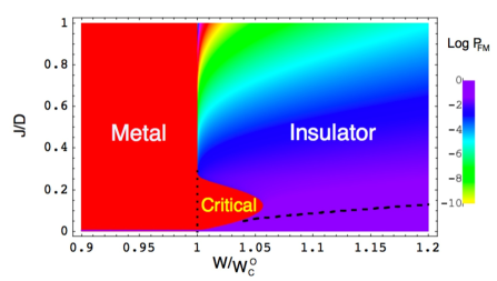
Figure 6: (Color online) The fraction of free magnetic moments $P_{\rm FM}$ at $T=0K$, Eq. (37), in a three-dimensional disordered metal as function of the exchange coupling $J$ (in units of the band width $D$) and disorder strength $W$ (in units of the critical value $W_{\rm c}^{\rm O}$). Critical correlations result in a finite $P_{\rm FM}$ even for large $J>J_{c}^{A}$ (dashed line]). For $J<J^{\ast}$, Eq. (50) there is a critical region for disorder amplitudes $W_{\rm c}^{\rm O}<W<W_{\rm c}(J)$, where $W_{c}(j=J/D)$ is given by Eq. (49). This figure was previously published by the authors in Ref. kettemann, .

VIII.2 Insulator Phase

On the insulating side of the AMIT the density of free magnetic moments is finite as given by Eq. (37). Therefore, the time reversal symmetry and the spin symmetry of the conduction electrons is broken in proportion to the spin relaxation rate $1/\tau_{s}$. This leads to a shift of the AMIT from $W_{c}^{\rm O}$ to $W^{I}_{c}(1/\tau_{s})$, which we will determine in the following.

Before proceeding we note that in a disordered system the spin relaxation rate is proportional to the local density of states $\rho(E,{\bf r})$ at position ${\bf r}$, since it is given by

$$\frac{1}{\tau_{s}(E,T,{\bf r})} = -\,n_{m}\,\Omega\frac{\rho(E,{\bf r})}{\nu}\left(t_{0}^{2}\,{\rm Im}\,G_{d}+\pi\rho\,t_{0}^{4}\,G_{d}^{2}\right)$$ (45)

$$= \frac{\rho(E,{\bf r})}{\nu}\frac{1}{\tau_{s}^{(0)}(E,T)},$$

with the propagator of a localized d-level in the Anderson model $G_{d}$.zarand Here, $1/\tau_{s}^{(0)}$ is the spin scattering rate in a clean system as given by Eq. (44). Thus, Eq. (45) leads us to conclude that the spin scattering rate not only depends on the ratio $T/T_{K}$ but also explicitly depends on the LDOS. Since both $T_{K}$ and $\rho(E,{\bf r})$ are randomly distributed, $1/\tau_{s}(E,T,{\bf r})$ is distributed as well.

In Section VI it was found that on the insulating side of the AMIT the LDOS at the position of unscreened magnetic moments scales as $\rho(\epsilon_{F},{\bf r})\sim\xi^{d-\alpha(J)}$, where $\alpha_{FM}=\alpha_{0}+dj$ is the critical value. Therefore, for $\alpha>\alpha_{FM}$ the magnetic moments remain free. According to Eq. (45) the spin relaxation rate due to the free moments depends itself on the localization length as

$$\frac{1}{\tau^{\rm FM}_{s}}(T=0) = 2\pi\,n_{\rm FM}(\xi)\,S(S+1)j^{2}\times$$ (46)

$$\rho(\epsilon_{F})\left(\frac{\xi}{a_{c}}\right)^{d-\alpha_{0}-dj},$$

where the density of free moments is given by Eq. (37) and, depends on the localization length $\xi$ as $n_{\rm FM}=n_{M}(\xi/a_{c})^{-\frac{d}{2\eta/d}j^{2}}$. Following Ref. larkin, , we get the critical disorder amplitude when the argument of the scaling function $g$ in Eq. (43) is of order unity, yielding the condition $D\tau_{s}(J)=\xi[W_{c}^{I}(J)-W_{\rm c}^{\rm O}]^{2}$ as function of the exchange coupling $J$. This condition is valid as long as the deviation from $W_{\rm c}^{\rm O}$ is small. For larger deviations it will converge to its unitary value $W_{\rm c}^{\rm U}$. The exact analytical form cannot be obtained from this phenomenological scaling approach. We note that, in contrast to the case of an external magnetic field, as considered in Ref. larkin, , according to Eq. (47), $\tau_{s}$ depends on the localization length $\xi$ as

$$\frac{1}{\tau^{\rm FM}_{s}}(T=0)=\frac{1}{\tau^{0}_{s}}\left(\frac{\xi}{a_{c}}\right)^{-\frac{d}{2\eta/d}(j+\eta/d)^{2}},$$ (47)

where

$$\frac{1}{\tau^{0}_{s}}=2\pi n_{M}S(S+1)j^{2}\rho(\epsilon_{F})$$ (48)

Thus, we finally get the shift of the critical disorder as function of $J$ as

$$W^{I}_{\rm c}(j)=W_{\rm c}^{\rm O}+W_{\rm c}^{\rm O}\left(\frac{a_{c}^{2}}{D_{e}\tau^{0}_{s}}\right)^{\kappa(j)},$$ (49)

where $1/\kappa(j)=\nu[2-\frac{d^{2}}{2\eta}(j+\eta/d)^{2}]$. This result is valid for small deviations from $W_{\rm c}^{\rm O}$. For larger deviations it will approach the unitary value $W_{\rm c}^{\rm U}$ in a still unknown form. We see that for $j=j^{\ast}$ where

$$j^{\ast}=\frac{2\sqrt{\eta}}{d}-\frac{\eta}{d},$$ (50)

which gives in $d=3$, $j^{\ast}\approx 0.276$, the exponent $\kappa(j)$ diverges and $W^{I}_{\rm c}$ approaches its orthogonal value $W_{\rm c}^{\rm O}$, see Fig. 6. Also, for larger values of $J$, it will stay at $W_{\rm c}^{\rm O}$ as a consequence of the increase of Kondo screening with the exchange coupling $J$.

VIII.3 Critical Semimetal Phase.

For smaller exchange couplings $j<j^{\ast}$ a paradoxical situation appears: The position of the critical point $W^{I}_{\rm c}$ depends on the direction from which the AMIT is approached. Therefore, for intermediate disorder strengths, $W_{\rm c}^{\rm O}<W<W^{I}_{\rm c}(j)$ there exists a critical region. Accordingly, the mobility edge is extended to a critical band whose width is a function of $j$. The resulting zero-temperature quantum phase diagram is shown in Fig. 6. According to Eq. (49) with Eq. (48), the width of the semimetal phase $W^{I}_{\rm c}(J)-W_{\rm c}^{\rm O}\sim n_{M}^{\kappa(j)}$ increases with a power of the density of magnetic impurities $n_{M}$.

IX Kondo-Anderson Transitions in a Magnetic Field

A Zeeman magnetic field polarizes the free magnetic moments. Thereby, their contribution to the spin relaxation rate becomes diminished by the magnetic field.bobkov ; vavilov ; micklitz On the other hand, the Kondo singlet which Kondo screened magnetic moments form with the conduction electrons is partially broken up by the Zeeman field. Thus, these magnetic moments contribute a spin relaxation rate which is increasing with the Zeeman field. Finally, an orbital magnetic field breaks the time reversal symmetry and therefore also results in a shift of the AMIT towards the unitary limit. It is therefore an intriguing problem how these competing magnetic field effects combine to change the quantum phase diagram.raikh

The magnetic field dependence of the spin relaxation rate from magnetic impurities in a metal at finite temperature was calculated in Ref. vavilov, . The magnetic field polarises the magnetic impurity spins due to the Zeeman interaction,

$$H_{Z}=-\gamma_{s}B\sum_{i}{S_{iz},}$$ (51)

where $\gamma_{s}=g_{s}\mu_{\rm B}$ is the gyromagnetic ratio of the magnetic impurities, $g_{s}$ their g-factor and $\mu_{\rm B}$ is Bohr’s magneton. Here, the magnetic field ${\bf B}$ is taken to point in the z-direction. The spin relaxation rate from free magnetic impurities is found to be exponentially suppressed according to $1/\tau_{s}\sim\exp(-\gamma_{s}B|S_{z}|/k_{\rm B}T)$. Thus, in the zero temperature limit all free moments are expected to become polarized by an arbitrarily small magnetic field, and their contribution to the spin relaxation is vanishing identically.

Magnetic impurities which are screened with a finite Kondo temperature $T_{K}$, however, have without magnetic field a spin relaxation rate Eq. (44) which vanishes in the low temperature limit. Applying a magnetic field the Kondo singlet is partially broken up and a finite spin relaxation rate appears, which scales with $T_{K}$ asvavilov ; micklitz

$$\frac{1}{\tau_{s}}(T_{K})=\frac{n_{M}}{\pi\rho}\frac{(\gamma_{s}B|S_{z}|)^{2}}{T_{K}^{2}}.$$ (52)

To get the total spin relaxation rate, we integrate over the distribution of Kondo temperatures $P(T_{K})$. We note that the contribution from magnetic impurities with a small Kondo temperature, $T_{K}<g_{s}\mu_{\rm B}B|S_{z}|$ vanishes since these spins become polarised. The ones with larger Kondo temperatures then yield the spin relaxation rate,

$$\frac{1}{\tau_{s}}=\int_{\gamma_{s}B|S_{z}|}^{\infty}dT_{K}P(T_{K})\frac{n_{M}}{\pi\rho}\frac{(\gamma_{s}B|S_{z}|)^{2}}{T_{K}^{2}}.$$ (53)

For small magnetic fields, $\gamma_{s}B|S_{z}|\ll T_{K}^{(0)}$, the main contribution comes from the low $T_{K}$-tail of the distribution,

$$P(T_{K})\sim\left(\frac{E_{c}}{T_{K}}\right)^{1-j}\xi^{-\frac{d^{2}}{2\eta}j^{2}}.$$ (54)

Thus, we get

$$\frac{1}{\tau_{s}}=\frac{n_{M}}{\pi\rho}\frac{dj}{2-j}\xi^{-\frac{d^{2}}{2\eta}(j+\eta/d)^{2}}\left(\frac{\gamma_{s}B|S_{z}|}{E_{c}}\right)^{j}.$$ (55)

Setting $X_{s}=\xi^{2}/D_{e}\tau_{s}=1$, we find that the Zeeman field shifts the critical disorder to

$$W_{c}(B)=W_{c}^{I}(j)+W_{c}^{O}c_{M}\left(\frac{\gamma_{s}B|S_{z}|}{E_{c}}\right)^{j\kappa(j)},$$ (56)

where $1/\kappa(j)=2\nu(1-\frac{d^{2}}{4\eta}(j+\eta/d)^{2})$ and $c_{M}=\left(djn_{M}/((2-j)\pi\rho D_{e})\right)^{\kappa(j)}$. Thus, the transition between critical semimetal and insulator is shifted in a magnetic field according to Eq. (56) as plotted in Fig. (7).

The orbital magnetic field is knownlarkin to shift $W_{c}$ to

$$W_{c}(B)=W_{c}^{O}+W_{c}^{O}(\pi eB/h)^{1/(2\nu)}.$$ (57)

This determines the transition line between metal and semimetal, since, the Zeeman field contributes a slower dependence on $B$, coming from the metal side of the transition we find $W_{c}(B)=W_{c}^{O}+W_{c}^{O}\left(\frac{\gamma_{s}B|S_{z}|}{E_{c}}\right)^{1/\nu}.$

For the transition between semimetal and insulator, we can conclude that for

$$j<j_{Z}=\eta/d\left(2\sqrt{d+1+d^{2}/\eta}/d-1-2/d\right),$$ (58)

the shift of $W_{c}$ is dominated by the Zeeman field over the orbital magnetic field. For, $d=3,\eta/d=2/3$ one finds, $j_{Z}=0.185$, so that the Zeeman field effect dominates for realistic values of exchange couplings $j$ as seen in Fig. (7).

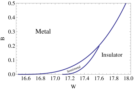
Figure 7: (Color online) The quantum phase diagram in a magnetic field $B$ (arbitrary units), as function of disorder amplitude $W$, in units of $t$. We set $d=3,\eta=2$ and $j=.2$.

X Finite Temperature Properties

We can now proceed to calculate finite temperature properties. To this end, we first derive the density of free magnetic moments at temperature $T$. It can be obtained by integrating $P(T_{K})$ according to

$$n_{FM}(T)=n_{M}\int_{0}^{T}dT_{K}P(T_{K}).$$ (59)

At low temperatures, $T\ll T_{K}^{0}$ the free moments are determined by the tail of the distribution.

X.1 Insulator

In the insulating regime for $T>\Delta_{\xi}$, $P(T_{K})$ is given by Eq. (25), while at smaller temperature, not exceeding the local level spacing, $T<\Delta_{\xi}$, the tail of $P(T_{K})$ is changing to Eq. (36). Thus we find the density of free moments in the insulating regime

$$n_{FM}(T)=n_{FM}(0)+n_{M}\left\{\begin{array}[]{cc}\frac{2d}{\eta}\left(\frac{T}{E_{c}}\right)^{\frac{\eta}{2d}}{\rm for}&T>\Delta_{\xi}\\ \frac{1}{j}\left(\frac{T}{E_{c}}\right)^{j\hskip 8.5359pt}\xi^{-\frac{1}{2\eta}(dj)^{2}}{\rm for}&T<\Delta_{\xi}\end{array}\right.,$$ (60)

where the density of free moments at $T=0$, $n_{FM}(0)$ is given by Eq. (37), decaying towards the AMIT. This result is plotted as function of disorder amplitude $W$ for various temperatures $T$ in Fig. (8). Thus, we find that the magnetic susceptibility is diverging at low temperature

$$\chi(T)=\frac{n_{FM}(T)}{T}\sim n_{FM}(0)\frac{1}{T}+$$

$$n_{M}\frac{1}{E_{c}}\left\{\begin{array}[]{cc}\frac{2d}{\eta}\left(\frac{T}{E_{c}}\right)^{\frac{\eta}{2d}-1}{\rm for}&T>\Delta_{\xi}\\ \frac{1}{j}\left(\frac{T}{E_{c}}\right)^{j-1\hskip 8.5359pt}\xi^{-\frac{1}{2\eta}(dj)^{2}}{\rm for}&T<\Delta_{\xi}\end{array}\right.,$$ (63)

with a Curie tail, whose weight increases as the Fermi energy moves deeper into the insulating regime. The specific heat is given by,

$$C(T)\sim T\frac{dn_{\rm FM}(T)}{dT}=n_{M}\left\{\begin{array}[]{cc}\left(\frac{T}{E_{c}}\right)^{\frac{\eta}{2d}}{\rm for}&T>\Delta_{\xi}\\ \left(\frac{T}{E_{c}}\right)^{j\hskip 8.5359pt}\xi^{-\frac{1}{2\eta}(dj)^{2}}{\rm for}&T<\Delta_{\xi}\end{array}\right..$$ (64)

These results also apply at the AMIT, where $n_{FM}(0)\rightarrow 0$ and $\Delta_{\xi}\rightarrow\Delta$.

X.2 Metal

In the metallic regime, $P(T_{K})$ is for $T<\Delta_{\xi}$ given by Eq. (32), so that we obtain,

$$n_{FM}(T)=n_{M}\frac{d}{\eta}\left(\frac{T}{E_{c}}\right)^{\frac{\eta}{2d}}\exp\left[-\frac{\Delta_{\xi}^{\frac{\eta}{d}}}{c_{1}}\ln(\frac{T}{T_{K}^{0}})^{2}\right],$$ (65)

Accordingly, we find that the magnetic susceptibility $\chi(T)=n_{FM}(T)/T$ has also in the metallic regime a power law tail, which is however cutoff at $T<\Delta_{\xi}$, where it converges to zero. We get the contribution to the specific heat, using $C(T)\sim T\frac{dn_{\rm FM}(T)}{dT}\sim n_{\rm FM}(T)$, vanishing at low temperatures $T\ll\Delta_{\xi}$.

One may ask if these thermodynamic results are modified by inelastic scatterings, introducing a thermal length $L_{T}$, which decreases with increasing temperature according to $L_{T}\sim T^{-1/z}$, where $z$ is the dynamical exponent. If electron-electron and electron-phonon scatterings are disregarded, $L_{T}$ is set by the relation $T=\Delta_{L_{T}}=D/L_{T}^{d}$, yielding $z=d$. Therefore, it has been argued that on length scales exceeding $L_{T}$, the system size $L$ and the localisation length/correlation lengths $\xi$ are substituted by $L_{T}$, in the scaling theory of the AMIT leeramakrishnan . Thus, indeed, for temperatures $T>\Delta_{\xi}$, $\xi$ would have to be substituted by $L_{T}$. However, as we find above, in this temperature range the results do not depend on $\xi$ anymore, so that the finite $L_{T}$ does not modify the above results.

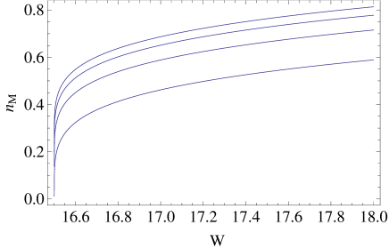
Figure 8: (Color online) The ratio of free magnetic moments (magnetic moments with $T_{K}<T$), $n_{FM}/n_{M}$, as function of disorder strength $W$ on the insultating side of the transition for temperatures $T/E_{c}=0,1\times 10^{-6},5\times 10^{-6},1\times 10^{-5}$ from the bottom to the top curve. We set $j=0.2$, $d=z=3$ and $\eta/d=2/3$.

XI Finite Temperature Phase Diagram: Kondo-Anderson Transitions

The spin relaxation rate is found to depend on temperature, Eq. (44), due to the Kondo screening, and the temperature dependence of the density of free magnetic moments, Eq. (60). Therefore, the amount by which the spin- and time-reversal-symmetry is broken, depends on temperature as well. Since the position of the AMIT is determined by these symmetries,ohtsukislevinreview it shifts as function of temperature $T$: when the spin relaxation rate increases with temperature, the AMIT shifts towards larger values of disorder amplitude $W$. Thus, a metal-insulator transition may occur at a finite temperature $T_{c}(W,J)$. In order to investigate the existence of such a transition, we will apply the Larkin-Khmel’nitskii condition larkin ; droese with the temperature dependent symmetry parameter $X_{s}(T)=\xi^{2}/D_{e}\tau_{s}(T)$. Since the condition $X_{s}=1$ gives an estimate for the position of the transition, $W_{c}(J,T)$, we find,

$$\left[\xi(W_{c}(J,T)\right]^{2}=a_{c}^{2}\left[\frac{W_{c}^{O}}{W_{c}(J,T)-W_{c}^{O}}\right]^{2\nu}=D_{e}\tau_{s}(J,T).$$ (66)

Again, as in the previous section, we can apply this criterion in two ways:

XI.1 Approaching the AMIT from the Insulator side.

Coming from the insulating side of the transition, where the localization length $\xi$ is still finite and smaller than the thermal length $L_{T}$, the ratio $X=\xi^{2}/D_{e}\tau_{s}(T)$ is finite, giving a measure of the amount of time reversal symmetry breaking. $1/\tau_{s}(T)$ saturates at low temperatures to the spin relaxation rate from free magnetic moments Eq. (47). Thus, at low temperatures the transition occurs at $W_{c}^{I}(J)$ as given by Eq. (49). At higher temperatures $1/\tau_{s}(T)$ increases with a power which depends on the distribution of the Kondo temperature. Thus, the spin relaxation rate at finite temperature is given by a weighted integral over the distribution function of $T_{K}$, as $1/\tau_{s}(T)=\int_{0}^{\infty}dT_{K}P(T_{K})1/\tau_{s}(T/T_{K})$. The spin relaxation rate of a magnetic impurity with a given Kondo temperature $T_{K}$, $1/\tau_{s}(T/T_{K})$, follows Eq. (44). Thus, it increases first like $T^{2}/T_{K}^{2}$ when $T<T_{K}$, until it reaches a maximum and then decays logarithmically slowly towards its classical value $1/\tau^{\rm classical}_{s}$. Since our analysis is limited to low temperatures $T\ll T^{0}_{K}$, we can simplify $1/\tau_{s}(T)$ as a sum of spin relaxation of free moments of density Eq. (60), at sites whose density of states is suppressed as $\rho({\bf r})\sim\xi^{d-\alpha_{FM}}$, and the spin relaxation from spins whose Kondo temperature exceeds $T$, which we can approximate by $T^{0}_{K}$ due to the peaked distribution. Thereby we get in good approximation the spin relaxation rate in the insulator as

$$\frac{1}{\tau_{s}}(T)=\frac{1}{\tau^{0}_{s}}\left(\xi^{d-\alpha_{0}-dj}\frac{n_{FM}(T)}{n_{M}}+\frac{T^{2}}{T^{02}_{K}}\frac{1-\frac{n_{FM}(T)}{n_{M}}}{S(S+1)\pi^{2}}\right).$$ (67)

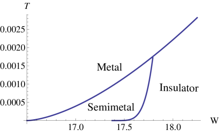
Figure 9: (Color online) The finite-temperature phase diagram of Kondo-Anderson transitions. The solid lines are plots of the critical temperatures $T_{c}^{M}(W,J)$, Eq. (70), and $T_{c}^{I}(W,J)$, Eq. (68), respectively, where the disorder amplitude $W$ is given in units of the hopping parameter $t$ and the temperature is in ratios of $E_{c}$. We used the following parameters: $j=0.2$, $\alpha_{0}=4$, $d=3$, $\eta/d=2/3$, $\nu=1.57$ and $a_{c}^{2}/(D_{e}\tau^{(0)}_{s})=0.1$.

When $X_{s}=1$ the symmetry breaking is sufficient to shift the transition to the larger disorder amplitude $W_{c}^{I}(J,T)$. Accordingly, we find the transition temperature,

$$T_{c}^{I}=E_{c}c_{I}\left(\frac{W-W_{c}^{I}}{W_{c}^{O}}\right)^{\frac{1}{j}},$$ (68)

where $W_{c}^{I}$ is given by Eq. (49), and $c_{I}=(\kappa_{j}/j)^{-1/j}(D_{e}\tau_{s}^{0})^{\kappa_{j}/j}$, where $1/\kappa_{j}=\nu(2-d^{2}/2/\eta(j+\eta/d)^{2})$.

XI.2 Approaching the AMIT from the Metallic side.

Coming from the metallic side, the density of free magnetic moments is decaying fast at temperatures $T<\Delta_{\xi}$ according to Eq. (65). Thus, the spin relaxation rate is dominated by the screened magnetic impurities, yielding,

$$\frac{1}{\tau_{s}}\approx\frac{1}{\tau^{0}_{s}}\frac{1}{S(S+1)\pi^{2}}\frac{T^{2}}{T_{K}^{02}},$$ (69)

where $1/\tau^{0}_{s}$ is given by Eq. (48). Thus, the transition is shifted to $W_{c}^{M}(T)$ and, accordingly, we find a transition temperature,

$$T_{c}^{M}(W)=\sqrt{S(S+1)\pi^{2}D_{e}\tau_{s}^{0}}\left|\frac{W-W_{c}^{O}}{W_{c}^{O}}\right|^{\nu}T_{K}^{0},$$ (70)

This is plotted in Fig. 9 as function of disorder amplitude $W$.

Thus, we can conclude that there is a critical semimetal region which extends over a finite temperature range, $T_{c}^{I}<T<T_{c}^{M}$. Since we derived the scaling function only at small symmetry breaking parameter $X_{s}$, the phase diagram at larger disorder, where the critical disorder of the unitary ensemble (when time-reversal symmetry completely broken) is approached, might be modified. This part of the phase diagram is further complicated by the fact that $1/\tau_{s}$ reaches a maximum and decays logarithmically at temperatures exceeding $T^{(0)}_{K}$. Furthermore, as inelastic scattering and dephasing processes will become stronger at higher temperatures, that higher temperature part of the phase boundaries is expected to become less well defined, mainly indicating a crossover region.

XII Conclusions and Discussion

We conclude that spin correlations in disordered metals do strongly modify the disorder induced Anderson metal-insulator transitions. Starting from the numerically well-established fact that a system of noninteracting electrons in a nonmagnetic disorder potential undergoes a second-order transition between a metallic state and an insulator, we studied the mutual influence of Kondo correlations and the Anderson localization transition. Since the position of the AMIT depends very strongly on time-reversal and spin symmetries, we find that the critical density and the critical disorder depend on the density of magnetic impurities, since these randomize the conduction electron spins. However, since the magnetic impurity spin in a metal is screened at low temperatures due to the Kondo effect, restoring a renormalized Fermi liquid with full time-reversal symmetry,nozieresfl we conclude that coming from the metallic side, the transition occurs at the critical disorder of a time-reversal invariant system, $W_{c}^{\rm O}$. However, coming from the insulating side, it occurs instead at the stronger critical disorder of a system where this symmetry is to some degree broken by free magnetic impurity spins. Since a shift in the AMIT results in an exponential change of the finite temperature resistivity, this has very strong experimental consequences. Since both the correlation length and the localization length are infinite in the critical region in-between the two critical points, the zero-temperature conductivity vanishes in this region, making the system a semimetal.

Taking into account the multifractality of the critical wave functions, we derived the concentration of unscreened magnetic impurities, the resulting spin scattering rate, and therefore the shift of the AMIT. Information on the multifractal distribution of the critical wave functions, which is well established by numerous careful numerical calculations,rmpmirlinevers allowed us also to characterize this critical region in more detail. Unscreened magnetic moments occur at sites with low intensity, which break the time-reversal symmetry of the conduction electrons. At sites with high intensity local singlets are formed, where one conduction electron is captured and localised, leaving the symmetry of the other conduction electrons unchanged. Thus, the Kondo-Anderson transitions share some features of a first-order phase transition: In the critical semimetal phase there is coexistence of different magnetic states of the magnetic impurity spins, which change the states of the conduction electrons, accordingly. A magnetic Zeeman fields is found to shift the transition to larger disorder $W$, and is dominating the magnetic field dependence for small exchange couplings $j<j_{z}$.

An experimental consequence of the critical semimetal phase is the divergence of the dielectric susceptibility, $\chi(T=0)\sim\xi^{2}\sim[W^{I}_{c}(J)-W]^{-2\nu}$ at the disorder amplitude $W^{I}_{c}(J)$ (or at a critical electron density $n^{I}_{c}(J)$), while the zero temperature limit of the resistivity diverges with the correlation length as $\rho(T=0)\sim\xi_{c}\sim(W-W_{c}^{\rm O})^{-\nu}$ at the weaker disorder amplitude $W_{c}^{\rm O}$ (or at a larger critical density $n_{c}^{\rm O}$, accordingly). This difference, $W^{I}_{c}(J)-W_{c}^{\rm O}$, increases with the concentration of Kondo impurities, as given by Eq. (49), until it converges to its limiting value $W^{U}_{c}-W_{c}^{\rm O}$.ohtsukislevinreview We expect the critical semimetallic phase to be observable in materials where both the AMIT and the Kondo effect are present simultaneously at experimentally accessible temperatures, such as in amorphous metal-semiconductor alloys kmck ; amormetal with dilute magnetic impurities,hasegawa or in doped semiconductors, such as Si:P, where thermopower measurements are consistent with the presence of Kondo impurities with $\langle T_{K}\rangle\approx 1K$.thermopower

On the insulating side of the transition, physical properties such as the finite-temperature resistivity are governed by the single-particle gap $\Delta_{c}=1/(\rho\xi^{d})=E_{c}[(W-W_{c}^{I})/W_{c}^{I}]^{\nu d}$, which causes activated behavior.

Aspects of the Kondo-Anderson transitions may be relevant for the understanding of metal-insulator transitions in real materials like Si:P. There have been detailed observations of a finite density of magnetic moments in Si:P across the transition, from magnetic susceptibility and specific heat measurements.loehneysen These have been previously modeled by the phenomenological two-fluid model of Refs. andres, ; paalanen, which did not take into account the Kondo effect. On the other hand, a realistic description of Si:P should consider that uncompensated Si:P contains a random array of half-filled donor levels that are randomly coupled. At low-donor concentration, close to the MIT, these levels are only weakly hybridized with the conduction band. Therefore, Si:P should at least be described by a half-filled Hubbard model with random hopping and on-site potentials.bhatt ; loehneysen ; paalanen Thus, all localized states carry single electrons with spin $1/2$ and double occupancy is prevented by the on-site interaction $U$. For the Hubbard model without disorder, the ground state at half filling is antiferromagnetic and there is an excitation gap of order $U$. Dynamical mean-field theory (DMFT) calculations show that, at least in the limit of infinite dimensions, spectral weight is transferred into the middle of the gap; it has been argued that these states yield extended quasiparticles which may form a Fermi liquid.nozieres2004 These quasiparticles interact with the localized magnetic moments in the lower Hubbard band, similarly to normal conduction electron quasiparticles which interact with magnetic Anderson impurities. In the presence of disorder, it has been shown that even when there are no resonant levels, and the donor levels have merged with the conduction band, the localized states in the band tail may carry localized magnetic moments.milovanovic Calculations of the disordered Hubbard model, using the statistical DMFT,Miranda ; mirandaprl and a variant of the local DMFT method byczuk show also that this model shares many features with the disordered Anderson impurity model studied in this article. As mentioned above, starting from the Anderson impurity model, we neglected the magnetic impurity scalar potential $K$ given in Eq. (9). We can justify this now, by referring to nonperturbative numerical studies of the Kondo effect with a pseudogap of power $r$ which find that, below the critical exchange coupling $J_{c}=rD$, a scalar scattering potential is irrelevant and the magnetic moment remains unscreened,pseudogap leaving our conclusion about the density of free moments unchanged. In the other case of power-law divergencies, which we find to occur in the multifractal states at sites with large intensiy ($\alpha<\alpha_{0}$), a nonperturbative renormalization group analysis shows that the on-site potential is irrelevant for all antiferromagnetic exchange coupling amplitudes,bulla leaving our conclusion on the formation of local singlets at such sites unchanged as well. At finite density of magnetic moments the indirect exchange coupling is in competition with the Kondo screening. In a disordered metal these couplings are widely distributed. In the vicinity of the AMIT, their distribution function can be calculated in a similar manner than the Kondo temperature, and this will be presented in the subsequent article Ref. rkkykondo, .

A nonphenomenological, analytical approach to the AMIT of interacting, disordered electrons is provided by field theoretical methods that typically employ the replica trick.mitspinfluctuations Decoupling the resulting action of interacting Grassmann fields with the Hubbard-Stratonovich transformation, a subsequent gradient expansion of the matrix fields results in the nonlinear sigma model,mitspinfluctuations ; rmpbelitzkirkpatrick . This kind of field theory treats the disorder scattering nonperturbatively and allows for a renormalization group analysis. It turns out that not only the conductance but also a frequency parameter and the spin density are renormalized. In particular, it has been found that the disordered electron system becomes unstable to local spin density fluctuations at the AMIT.mitspinfluctuations It is still unclear if these indicate the onset of a magnetic phase transition,chamon00 ; nayak03 or are rather precursors of the formation of local magnetic moments.rmpbelitzkirkpatrick Since the nonlinear sigma model is formulated in order to account for long wavelength fluctuations such as charge diffusion and spin diffusion modes, it cannot, at least in these early formulations, describe local moment formation. Therefore, it is an open challenge, to combine the field-theoretical approach to the AMIT with a nonperturbative treatment of the local moment formation and the Kondo correlations caused by them. Field theoretical formulations of the disordered Kondo problem have been developed in the mean field approximation,burdin ; kim and in the Ginzburg-Landau theory.kiselev ; coqblin However, in these approaches, the AMIT of the conduction electrons in the disordered potential has not yet been taken into account. We hope that the theory of the Kondo-Anderson transitions presented in this paper, which was based, to some extent phenomenologically, on the multifractal distributions and correlations at AMITs, can serve as a guide in the quest for a theory, which is derived from the Hamiltonian of disordered, interacting electrons, taking into account nonperturbatively both disorder and interaction effects, including Kondo correlations.

XIII Acknowledgements

We gratefully acknowledge useful discussions with Elihu Abrahams, Ravin Bhatt, Georges Bouzerar, Vladimir Dobrosavljevic, Alexander M. Finkel’stein, Serge Florens, Hilbert von Löhneysen, Philippe Nozières, Mikhail Raikh, and Gergely Zarand. This research was supported by WCU(World Class University) program through the National Research Foundation of Korea funded by the Ministry of Education, Science and Technology(R31-2008-000-10059-0), Division of Advanced Materials Science. This work was partially financed by the Hungarian Research Fund (OTKA) grant K73361 and the Alexander von Humboldt Foundation. ERM, KS and IV thank the WCU AMS and APCTP for its hospitality. SK thanks the ILL Grenoble for its hospitality.

Appendix A Wave function Correlations in the vicinity of the AMIT

A.1 One Energy at the mobility edge $E_{M}$.

The long-range spectral correlations in a $d$-dimensional system can be quantified by spatially integrating the correlation function of the eigenfunction probabilities associated to two energy levels distant by $\omega_{nm}=E_{n}-E_{m}$.ioffe When one of these energies is at the mobility edge $E_{M}$, one finds

$$C_{nm} = L^{d}\int d^{d}r\,\left\langle|\psi_{n}({\bf r})|^{2}|\psi_{m}({\bf r})|^{2}\right\rangle$$ (73)

$$= \left\{\begin{array}[]{ll}(\frac{E_{c}}{{\rm Max}(|\omega_{nm}|,\Delta)})^{\eta/d},&0<|\omega_{nm}|<E_{c},\\ (E_{c}/|\omega_{nm}|)^{2},&E_{p}>|\omega_{nm}|>E_{c},\end{array}\right.$$

where $0<\eta<d$, with $\eta=2(\alpha_{0}-d)$. This exponent is obtained by the requirement that in the limit of small energy differences, $|\omega_{nm}|\rightarrow\Delta$, one recovers

$$C_{nm}|_{|\omega_{nm}|\rightarrow\Delta}\rightarrow L^{2d}\left\langle|\psi_{n}({\bf r})|^{4}\right\rangle\sim L^{d-\tau_{2}},$$ (74)

where $\tau_{2}=d_{2}=d-2(\alpha_{0}-d)$ and $\Delta=D/L^{d}$. For $|\omega_{nm}|<E_{c}$, correlations are enhanced in comparison to the plane-wave limit, where $C_{nm}=1$. Note that for $|\omega_{nm}|>E_{c}$ the correlation function decays below $1$. This anticorrelation ensures that the intensity is normalised: A dip in the intensity at one energy implies an enhancement of intensity at another energy in the band. This anticorrelation is expected to occur up to some finite energy $E_{p}$, beyond which the correlation function increases to the uncorrelated value $1$ in a nonuniversal way.

A.2 Both energies at a distance from the mobility edge $E_{M}$.

The spectral correlations in a $d$-dimensional system also exist away from the transition whenever either the correlation length $\xi$ (on the metallic side) or the localization length $\xi_{c}$ (on the insulator side) are finite. In the correlation function of Eq. (73), the energy difference $|\omega_{nm}|$ is for $\epsilon_{n}<\epsilon_{m}$ then substituted by ${\rm Max}[|\omega_{nm}|,\Delta_{\xi_{n}}]$, where $\Delta_{\xi_{n}}=E_{c}\,(\xi_{n}/a_{c})^{-d}$, and $a_{c}$ is defined by $E_{c}=1/(\rho a_{c}^{d})$, with $\rho$ denoting the average density of states. We get therefore

$$C_{nm} = L^{d}\int d^{d}r\,\left\langle|\psi_{n}({\bf r})|^{2}|\psi_{m}({\bf r})|^{2}\right\rangle$$ (77)

$$= \left\{\begin{array}[]{ll}\left[\frac{E_{c}}{{\rm Max}[|\omega_{nm}|,\Delta_{\xi_{n}}]}\right]^{\eta/d},&0<|\omega_{nm}|<E_{c},\\ \left(\frac{E_{c}}{|\omega_{nm}|}\right)^{2},&|\omega_{nm}|>E_{c},\end{array}\right.$$

where $\eta=2(\alpha_{0}-d)$. For $\omega_{nm}<E_{c}$, correlations are still enhanced in comparison to the plane-wave limit, where $C_{nm}=1$.

A.3 Joint Distribution Function.

The joint distribution function of two eigenfunction intensities at the same position should be log-normal since the distribution function of a single eigenfunction intensity is log-normal as given by Eq. (2). Therefore, we recently conjectured it recently to be of a log-normal form, when one of the energies is at the mobility edge.kettemann In general, when, one or both energies are away from the mobility edge, the finite correlation length/ localisation length $\xi$ needs to be taken into account when one or both energies are on the metallic/localised side of the transition, respectively. We can then conjecture the joint distribution function for $\alpha_{l}$ and $\alpha_{k}$, where, in the metallic regime, we define $\alpha=-\frac{\ln[(L/\xi)^{d}|\psi(x)|^{2}]}{\ln\xi},$ which has the distribution $P(\alpha)\sim\xi^{-(\alpha-\alpha_{0})^{2}/(2\eta)}$. Accordingly, in the localized regime, we get the same distribution function, defining there $\alpha=-\ln[|\psi(x)|^{2}]/\ln\xi$. Then, for $|\epsilon_{l}-\epsilon_{k}|<E_{c}$, we conjecture the joint distribution function to be of the form,

$$P(\alpha_{l},\alpha_{k})=\xi_{l}^{a_{lk}\left[f(\alpha_{l})-d\right]}\xi_{k}^{a_{lk}\left[f(\alpha_{k})-d\right]}K_{lk}^{-a_{lk}\frac{(\alpha_{l}-\alpha_{0})(\alpha_{k}-\alpha_{0})}{d\eta}},$$ (78)

where $\xi_{l}$ is the correlation/localization length of a state at energy $E_{l}$, $K_{{lk}}={\rm Max}\left[|E_{l}-E_{k}|,{\rm Min}(\Delta_{\xi_{l}},\Delta_{\xi_{k}})\right]/E_{c}$, and

$$a_{lk}=\frac{1}{1-\left(\frac{\ln K_{lk}}{d\ln\hat{\xi}}\right)^{2}},$$ (79)

where we introduced the length scale $\hat{\xi}$ through

$$\ln\hat{\xi}=\sqrt{\ln\xi_{l}\ln\xi_{k}}.$$ (80)

Averaging the local intensity of the state with energy $E_{l}$ with the conditional probability $P(\alpha,\alpha_{l})/P(\alpha)$, which can be rewritten as

$$P_{\alpha_{k}=\alpha}(\alpha_{l})=\xi_{l}^{-a_{lk}\frac{[\alpha_{l}-\alpha_{0}+\frac{\ln K_{lk}}{d\ln\xi_{l}}(\alpha-\alpha_{0})]^{2}}{2\eta}},$$ (81)

we then get Eq. (28),

$$I_{\alpha{\rm}}(\xi_{l},\xi_{k})=\langle L^{d}|\psi_{l}({\bf r})|^{2}\rangle_{\alpha}=K_{lk}^{\frac{\alpha-\alpha_{0}}{d}-\frac{\eta}{2d^{2}}\frac{\ln K_{lk}}{\ln\xi_{k}}}.$$ (82)

Note that when the energy $E_{k}$ is at the mobility edge $E_{k}=E_{M}$ then $\xi_{k}\rightarrow L$, in Eq. (78), and we recover the conditional intensity at energy $E_{l}$, Eq. (5), in a more rigourous way (the finite correlation length of that state, $\xi_{l}$, did not appear explicitly in our previous conjecture Eq. (7) of Ref. kettemann, , but is now taken into account in Eq. (78)).

A.4 Higher Moment Correlation Functions

The correlation of higher moments of the intensities is defined by

$$C^{q}_{\{n_{i}\}} = L^{qd}\left\langle\prod_{i=1}^{q}|\psi_{n_{i}}({\bf r})|^{2}\right\rangle.$$ (83)

We consider first the case, where, one of the energies is fixed to the mobility edge, $E_{n_{1}}=E_{M}$. The power law of the correlation of higher moments of the intensity, can then be obtained by taking the limit of small energy differences, $\omega_{n_{i},n_{j}}\rightarrow\Delta$, which yields,

$$C^{q}_{\{n_{i}\}}\mid_{\omega_{n_{i},n_{j}}\rightarrow\Delta,\forall i} = L^{qd}\left\langle|\psi_{n}({\bf r})|^{2q}\right\rangle$$ (84)

$$\sim L^{(q-1)d-\tau_{q}}\sim L^{\eta_{q}}.$$

$\tau_{q}$ is found to terminate for $q>q_{c}=\alpha_{0}/\eta$. Thus, for $d=3$ and $\alpha_{0}=4$, $q_{c}=2$, so that all higher order moments have the same $\tau_{q}=\tau_{2}=d-\eta,\forall q>q_{c}$. Thus we find

$$\eta_{q}=(q-2)d+\eta.$$ (85)

Furthermore, we notice that the pair of intensities whose energy are closest to each other are correlated with a power $\eta/d$. Thus, we can conclude that the 3-rd order correlation function is to leading order given by

$$C^{3}_{\{n_{i}\}}\sim\left(\frac{E_{c}}{|{\rm Min}(\omega_{n_{i},n_{j}})|}\right)^{\frac{\eta}{d}}\frac{E_{c}}{|{\rm Max}(\omega_{n_{i},n_{j}})|}.$$ (86)

This result is valid for $0<|\omega_{n_{i},n_{j}}|<E_{c}\forall i,j$. If all energies in $C^{3}$ are placed away from the mobility edge, $E_{n_{1}}\neq E_{M}$, then the energy difference $|{\rm Min}(\omega_{n_{i},n_{j}})|$, is replaced by $\Delta_{n_{i}}=E_{c}/\xi_{n_{i}}^{d}$ if it is smaller than that energy scale, respectively.

Appendix B $F[\alpha,T_{K}]$

Let us first consider the case, when the Fermi energy is at the mobility edge. We can then evaluate $F[\alpha,T_{K}]$ in the following way. We transform the summation over states $l$ to the integration over energy $\epsilon$. Then, we transform to $t=-\ln(\epsilon/E_{c})$. Next, we can substitute in good approximation $\tanh x\approx x$ for $0<x<1$, and $\tanh x\approx 1$ for $x>1$. Thereby, we get

$$F[\alpha,T_{K}]=j\left(\int_{\ln(E_{c}/T_{K})}^{\ln(E_{c}/\Delta)}dte^{-t}+\int^{\ln(E_{c}/T_{K})}_{0}dt\right)$$

$$\times\exp[-\frac{\alpha-\alpha_{0}}{d}t-\frac{\alpha_{0}-d}{d^{2}}\frac{t^{2}}{\ln L}].$$ (87)

The integrals can now be performed, yielding Error functions, $\int_{a}^{b}e^{-At^{2}-Bt}=e^{B^{2}/(4A)}\frac{\sqrt{\pi}}{2\sqrt{A}}(Erf[\sqrt{A}b+B/(2\sqrt{A}))]-Erf[\sqrt{A}a+B/(2\sqrt{A}))])$, for each term in Eq. (B). Since $A=(\alpha_{0}-d)/(d^{2}\ln L)$ the arguments of all Error functions diverge for $L\rightarrow\infty$, and we can use the asymptotic expansion $Erf[z]\rightarrow{\rm sign}z\times 1-e^{-z^{2}}/(\sqrt{\pi}z)$. Thereby, we find for $\alpha>\alpha_{0}-d$,

$$F[\alpha,T_{K}]/j = \frac{d}{\alpha-\alpha_{0}}+\left(\frac{d}{2\alpha-\eta}-\frac{d}{\alpha-\alpha_{0}}\right)\left(\frac{E_{c}}{T_{K}}\right)^{\frac{\alpha_{0}-\alpha}{d}}$$ (88)

$$- d_{\alpha}\frac{E_{c}}{T_{K}}L^{-\alpha},$$

where $d_{\alpha}=d/(\eta+2\alpha)$. Solving $1=F[\alpha,T_{K}]$ we obatin then for $L\rightarrow\infty$, Eq. (13) for $T_{K}(\alpha)$.

References

- (1) R. N. Bhatt and D. S. Fisher, Phys. Rev. Lett. 68, 3072 (1992).
- (2) A. Langenfeld and P. Wölfle, Ann. Physik 4, 43 (1995).
- (3) V. Dobrosavljevic, T. R. Kirkpatrick, and G. Kotliar, Phys. Rev. Lett. 69, 1113 (1992); E. Miranda, V. Dobrosavljevic, and G. Kotliar, ibid. 78, 290 (1997).
- (4) E. Miranda and V. Dobrosavljevic, Rep. Prog. Phys. 68, 2337 (2005).
- (5) I. V. Lerner, Phys. Lett. A 133, 253 (1988).
- (6) S. Kettemann and E. R. Mucciolo, Pisma Zh. Eksp. Teor. Fiz. 83, 284 (2006) [JETP Lett. 83, 240 ( 2006)]; S. Kettemann and E. R. Mucciolo, Phys. Rev. B 75, 184407 (2007)
- (7) T. Micklitz, A. Altland, T. A. Costi, and A. Rosch, Phys. Rev. Lett. 96, 226601 (2006); T. Micklitz, T. A. Costi, and A. Rosch, Phys. Rev. B 75, 054406 (2007).
- (8) P. S. Cornaglia, D. R. Grempel, and C. A. Balseiro, Phys. Rev. Lett. 96, 117209 (2006).
- (9) I. Varga, E. R. Mucciolo, and S. Kettemann, International Journal of Modern Physics: Conference Series, Vol. x, to be published (2012).
- (10) A. Zhuravlev, I. Zharekeshev, E. Gorelov, A. I. Lichtenstein, E. R. Mucciolo, and S. Kettemann, Phys. Rev. Lett. 99, 247202 (2007).
- (11) F. Wegner, Z. Phys. B 36, 209 (1980); H. Aoki, J. Phys. C 16, L205 (1983); C. Castellani and L. Peliti, J. Phys. A 19, L991 (1986); M. Schreiber and H. Grußbach, Phys. Rev. Lett. 67, 607 (1991); M. Janssen, Int. J. Mod. Phys. B 8, 943 (1994).
- (12) F. Evers and A. D. Mirlin, Rev. Mod. Phys. 80, 1355 (2008).
- (13) L. J. Vasquez, A. Rodriguez, and R. A. Romer, Phys. Rev. B 78, 195106 (2008).
- (14) M. A. Ruderman and C. Kittel, Phys. Rev. 96, 99 (1954); T. Kasuya, Prog. Theor. Phys. 16, 45 (1956); K. Yosida, Phys. Rev. 106, 893 (1957).
- (15) A. I. Liechtenstein, M. I. Katsnelson, V. P. Antropov, and V. A. Gubanov, J. Magn. Magn. Mater. 67, 65 (1987).
- (16) S. Kettemann, K. Slevin, E. Mucciolo, unpublished (2011).
- (17) J. T. Chalker, Physica A (Amsterdam) 167, 253 (1990); V. E. Kravtsov and K. A. Muttalib, Phys. Rev. Lett. 79, 1913 (1997); J. T. Chalker et al., JETP Lett. 64, 386 (1996); T. Brandes, B. Huckestein, L. Schweiser, Ann. Phys. (Leipzig) 5, 633 (1996); V. E. Kravtsov, ibid. 8, 621 (1999); V. E. Kravtsov, A. Ossipov, O. M. Yevtushenko, and E. Cuevas, Phys. Rev. B 82, 161102 (2010); V. E. Kravtsov, A. Ossipov, O. M. Yevtushenko, J. Phys. A 44, 305003 (2011).
- (18) E. Cuevas and V. E. Kravtsov, Phys. Rev. B 76, 235119 (2007).
- (19) M. V. Feigel’man, L. B. Ioffe, V. E. Kravtsov, and E. A. Yuzbashyan, Phys. Rev. Lett. 98, 027001 (2007).
- (20) M. V. Feigel’man, L. B. Ioffe, V. E. Kravtsov, E. Cuevas, Annals of Physics 325, 1368 (2010).
- (21) S. Kettemann, E. R. Mucciolo, and I. Varga, Phys. Rev. Lett. 103, 126401 (2009).
- (22) A. D. Mirlin, Phys. Rep. 326, 259 (2000).
- (23) P. W. Anderson, Phys. Rev. 124, 41(1961).
- (24) A. C. Hewson, The Kondo Problem to Heavy Fermions (Cambridge University Press, Cambridge, 1997).
- (25) D. Withoff and E. Fradkin, Phys. Rev. Lett. 64, 1835 (1990); K. Ingersent, Phys. Rev. B 54, 11936 (1996); S. Florens, M. Vojta, Phys. Rev. B 72, 115117 (2005). L. Fritz, S. Florens, and M. Vojta, Phys. Rev. B 74, 144410 (2006).
- (26) Y. Nagaoka, Phys. Rev. 138, 1112 (1965); H. Suhl, Phys. Rev. A 138, 515 (1965).
- (27) G. Zarand and L. Udvardi, Phys. Rev. B 54, 7606 (1996).
- (28) For simplicity, we restrict here the integration interval to . Since the integration should actually be extended upto the band edges, the Kondo temperature we obtain is accordingly smaller by a constant factor. Since we rescale all results with the Kondo temperature of a clean system, , as obtained in the same approximation, this approximation does not effect any of the results reported here.
- (29) M. Vojta, and R. Bulla, Eur. Phys. J. B 28, 283 (2002).
- (30) A. MacKinnon and B. Kramer, Phys. Rev. Lett. 47, 1546 (1981); A. MacKinnon, and B. Kramer, Zeitschrift f. Physik B 53, 1 (1983).
- (31) S. Kettemann and M. E. Raikh, Phys. Rev. Lett. 90, 146601 (2003).
- (32) D. Khmelnitskii and A. I. Larkin, Solid State Comm. 39, 1069 (1981).
- (33) T. Dröse, M. Batsch, I. Kh. Zharekeshev, and B. Kramer, Phys. Rev. B 57, 37 (1998).
- (34) F. J. Wegner, Nuclear Physics B270 [FS16] , 1(1986).
- (35) S. Hikami, A. I. Larkin, and Y. Nagaoka, Prog. Theor. Phys. 63, 707 (1980).
- (36) M. A. Paalanen, T. F. Rosenbaum, G. A. Thomas, and R. N. Bhatt, Phys. Rev. Lett. 51, 1896 (1983).
- (37) P. A. Lee and T. V. Ramakrishnan, Rev. Mod. Phys. 57, 287 (1985).
- (38) G. Bergmann, Phys. Rev. Lett. 58, 1236 (1987); R. P. Peters, G. Bergmann, and R. M. Mueller, ibid. 58, 1964 (1987); C. Van Haesendonck, J. Vranken, and Y. Bruynseraede, ibid. 58, 1968 (1987).
- (39) P. Mohanty and R. A. Webb, Phys. Rev. Lett. 84, 4481 (2000).
- (40) G. Zaránd, L. Borda, J. von Delft, and N. Andrei, Phys. Rev. Lett. 93, 107204 (2004).
- (41) P. Nozières, J. Low Temp. Phys. 17, 3 (1974).
- (42) A finite magnetic scattering rate may arise on the metallic side when clusters of magnetic impurities form. However, their probability and the resulting magnetic scattering rate scale with the th power of the density of magnetic impurities,boucai and therefore are negligible for dilute systems.
- (43) E. Boucai, B. Lecoanet, J. Pilon, J. L. Tholence, and R. Tournier, Phys. Rev. B 3, 3834 (1971).
- (44) T. Ohtsuki and T. Kawarabayashi, J. Phys. Soc. Jpn. 66, 314 (1997); T. Ohtsuki, K. Slevin, and T. Kawarabayashi, Ann. Physik 8, 655 (1999).
- (45) A. Rodriguez, L. J. Vasquez, K. Slevin, R. A. Roemer, Phys. Rev. B 84, 134209 (2011).
- (46) A.A. Bobkov, V.I. Fal ko, and D.E. Khmel nitskii, Zh. Exp. Teor. Fiz. 98, 703 (1990) [Sov. Phys. JETP 71, 393 (1990)].
- (47) M.G. Vavilov, L.I. Glazman, Phys. Rev. B 67, 115310 (2003); M. G. Vavilov, L. I. Glazman, and A. I. Larkin, Phys. Rev. B 68, 075119 (2003).
- (48) We thank M. Raikh for asking us this question.
- (49) K. Andres, R. N. Bhatt, P. Goalwin, T. M. Rice, and R. E. Walstedt, Phys. Rev. B 24, 244 (1981) .
- (50) Note that we could get a more accurate result by integrating Eq. (44) , weighted by the distribution of , Eq. (36) in the localized regime. The result for low temperatures will not be strongly changed from the following result, however.
- (51) C. Van Haesendonck and Y. Bruynseraede, Phys. Rev. B 33, 1684 (1986); B. W. Dodson, W. L. McMillan, J. M. Mochel, and R. C. Dynes, Phys. Rev. Lett. 46, 46 (1981).
- (52) B. Kramer, A. MacKinnon, Rep. Prog. Phys. 56, 1469 (1993).
- (53) C. C. Tsuei and R. Hasegawa, Solid State Commun. 7, 1581 (1969).
- (54) M. Lakner and H. v. Löhneysen, Phys. Rev. Lett. 70, 3475 (1993).
- (55) H. v. Löhneysen, Adv. in Solid State Phys. 40, 143 (2000).
- (56) A. M. Finkel’shtein, JETP Lett. 46, 513 (1987).
- (57) M. A. Paalanen, S. Sachdev, R. N. Bhatt, and A. E. Ruckenstein, Phys. Rev. Lett. 57, 2061 (1986).
- (58) M. A. Paalanen, J. E. Graebner, R. N. Bhatt, and S. Sachdev, Phys. Rev. Lett. 61, 597 (1988); S. Sachdev, Phys. Rev. B 39, 5297 (1989).
- (59) P. Nozieres, J. Stat. Phys. 115, 19 (2004).
- (60) M. Milovanovic, S. Sachdev, and R. N. Bhatt, Phys. Rev. Lett. 63, 82 (1989).
- (61) E. Miranda and V. Dobrosavljevic, Phys. Rev. Lett. 86, 264 (2001); M. C. O. Aguiar, V. Dobrosavljevic, E. Abrahams, and G. Kotliar, Phys. Rev. Lett. 102, 156402 (2009).
- (62) K. Sato, L. Bergqvist, J. Kudrnovsky, P. H. Dederichs, O. Eriksson, I. Turek, B. Sanyal, G. Bouzerar, H. Katayama-Yoshida, V. A. Dinh, T. Fukushima, H. Kizaki and R. Zeller, Rev. Mod. Phys. 82, 1633 (2010).
- (63) K. Byczuk, W. Hofstetter, U. Yu, and D. Vollhardt, Eur. Phys. J. Special Topics 180, 135 (2010).
- (64) A. M. Finkel’stein, JETP Lett. 37, 517 (1983); ibid. 40, 796 (1984).
- (65) D. Belitz and T. R. Kirkpatrick, Rev. Mod. Phys. 66, 261 (1994).
- (66) C. Chamon and E. R. Mucciolo, Phys. Rev. Lett. 85, 5607 (2000).
- (67) C. Nayak and X. Yang Phys. Rev. B 68, 104423 (2003).
- (68) S. Burdin, and P. Fulde, Phys. Rev. B 76, 104425 (2007).
- (69) M.-T. Tran and K.-S. Kim, Phys. Rev. Lett. 105, 116403 (2010); J. Phys. Condens. Matter 23, 425602 (2011).
- (70) M. N. Kiselev, K. Kikoin, and R. Oppermann, Phys. Rev. B 65, 184410 (2002).
- (71) S. G. Magalhaes, F. M. Zimmer, B. Coqblin, Phys. Rev. B 81, 094424 (2010); B. Coqblin, J. R. Iglesias, N. B. Perkins, S. G. Magalhaes, F. M. Zimmer, J. Magn. Magn. Mater. 320, 1989 (2008).