Characterizing $W^{2,p}$ submanifolds by $p$-integrability of global curvatures

Abstract

We give sufficient and necessary geometric conditions, guaranteeing that an immersed compact closed manifold $\Sigma^{m}\subset{\mathbb{R}}^{n}$ of class $C^{1}$ and of arbitrary dimension and codimension (or, more generally, an Ahlfors-regular compact set $\Sigma$ satisfying a mild general condition relating the size of holes in $\Sigma$ to the flatness of $\Sigma$ measured in terms of beta numbers) is in fact an embedded manifold of class $C^{1,\tau}\cap W^{2,p}$, where $p>m$ and $\tau=1-m/p$. The results are based on a careful analysis of Morrey estimates for integral curvature–like energies, with integrands expressed geometrically, in terms of functions that are designed to measure either (a) the shape of simplices with vertices on $\Sigma$ or (b) the size of spheres tangent to $\Sigma$ at one point and passing through another point of $\Sigma$.

Appropriately defined maximal functions of such integrands turn out to be of class $L^{p}(\Sigma)$ for $p>m$ if and only if the local graph representations of $\Sigma$ have second order derivatives in $L^{p}$ and $\Sigma$ is embedded. There are two ingredients behind this result. One of them is an equivalent definition of Sobolev spaces, widely used nowadays in analysis on metric spaces. The second one is a careful analysis of local Reifenberg flatness (and of the decay of functions measuring that flatness) for sets with finite curvature energies. In addition, for the geometric curvature energy involving tangent spheres we provide a nontrivial lower bound that is attained if and only if the admissible set $\Sigma$ is a round sphere.

MSC 2000: 28A75, 46E35, 53A07

1 Introduction

In this paper we address the following question: under what circumstances is a compact, $m$-dimensional set $\Sigma$ in ${\mathbb{R}}^{n}$, satisfying some mild additional assumptions, an $m$-dimensional embedded manifold of class $W^{2,p}$? For $p>m=\dim\Sigma$ we formulate two necessary and sufficient criteria for a positive answer. Each of them says that $\Sigma$ is an embedded manifold of class $W^{2,p}$ if and only if a certain geometrically defined integrand is of class $L^{p}$ with respect to the $m$-dimensional Hausdorff measure on $\Sigma$. One of these integrands measures the flatness of all $(m+1)$-dimensional simplices with one vertex at a fixed point of $\Sigma$ and other vertices elsewhere on $\Sigma$; see Definition 1.2. The other one measures the size of all spheres that touch an $m$-plane passing through a fixed point of $\Sigma$ and contain another (arbitrary) point of $\Sigma$ (Definition 1.3).

The extra assumptions we impose on the set $\Sigma$ are: (1) Ahlfors regularity with respect to the $m$-dimensional Hausdorff measure $\mathscr{H}^{m}$, and (2) roughly speaking, a certain relation between the flatness of $\Sigma$ and the size of “holes” it might have: the flatter $\Sigma$ is, the smaller these holes must be. To state the main result, Theorem 1.4, formally, let us first specify these two conditions precisely and then define the geometric integrands mentioned above. Throughout the paper we denote with $\mathbb{B}^{n}(a,s)$ an open $n$-dimensional ball of radius $s$ centered at the point $a\in{\mathbb{R}}^{n}$, and we write $a\approx b$ if $a/C\leq b\leq Ca$ for some constant $C\geq 1$, and $a\lesssim b$ (or $a\gtrsim b$), if only the left (or right) of these inequalities holds.

1.1 Statement of results

Definition 1.1 (the class of $m$-fine sets).

Let $\Sigma\subset{\mathbb{R}}^{n}$ be compact. We call $\Sigma$ an $m$-fine set and write $\Sigma\in\mathscr{F}(m)$ if there exist constants $A_{\Sigma}>0$ and $M_{\Sigma}\geq 2$ such that

1. (Ahlfors regularity) for all $x\in\Sigma$ and $r\leq\mathop{\rm diam}\nolimits\Sigma$ we have

   $$\mathscr{H}^{m}(\Sigma\cap\mathbb{B}^{n}(x,r))\geq A_{\Sigma}r^{m}\,;$$ (1.1)

2. (control of “holes” in small scales) for each $x\in\Sigma$ and $r\leq\mathop{\rm diam}\nolimits\Sigma$ we have

   $$\theta_{\Sigma}(x,r)\leq M_{\Sigma}\,\beta_{\Sigma}(x,r)\,.$$

Here, $\beta_{\Sigma}$ and $\theta_{\Sigma}$ denote, respectively, the beta numbers and the bilateral beta numbers of $\Sigma$, defined by

$$\beta_{\Sigma}(x,r) :=\frac{1}{r}\inf\left\{\sup_{z\in\Sigma\cap\mathbb{B}(x,r)}\mathop{\rm dist}\nolimits(z,x+H):H\in G(n,m)\right\},$$ (1.2)

$$\theta_{\Sigma}(x,r) :=\frac{1}{r}\inf\Bigl{\{}d_{\mathscr{H}}(\Sigma\cap\overline{\mathbb{B}}(x,r),(x+H)\cap\overline{\mathbb{B}}(x,r)):H\in G(n,m)\Bigr{\}}\,,$$ (1.3)

where $G(n,m)$ stands for the Grassmannian of all $m$-dimensional linear subspaces of ${\mathbb{R}}^{n}$, and where

$$d_{\mathscr{H}}(E,F):=\sup\{\mathop{\rm dist}\nolimits(y,F):y\in E\}+\sup\{\mathop{\rm dist}\nolimits(z,E):z\in F\}$$

is the Hausdorff distance of sets in ${\mathbb{R}}^{n}$. Intuitively, condition (ii) of Definition 1.1 ascertains that if $\Sigma$ is flat at some scale $r>0$, then the gaps and holes in $\Sigma$ cannot be large. Their sizes are at most comparable to the degree of flatness of $\Sigma$. If an $m$-fine set $\Sigma$ satisfies $\beta_{\Sigma}(x,r)\to 0$ uniformly w.r.t $x\in\Sigma$ as $r\to 0$, then $\Sigma$ is Reifenberg flat with vanishing constant, see e.g. G. David, C. Kenig and T. Toro [5, Definition 1.3] for a definition. However, note that neither the Reifenberg flatness of $\Sigma$, nor rectifiability of $\Sigma$ itself is required in Definition 1.1. Both these properties follow from the finiteness of geometric curvature energies we consider here.

It is relatively easy to see that $\mathscr{F}(m)$ contains immersed $C^{1}$ submanifolds of ${\mathbb{R}}^{n}$ (cf. [16, Example 1.60] for a short proof), or embedded Lipschitz submanifolds without boundary. It also contains other sets such as the following stack of spheres $\Sigma=\bigcup_{i=0}^{\infty}\Sigma_{i}\cup\{0\}$, where the $2$-spheres $\Sigma_{i}={\mathbb{S}}^{2}(c_{i},r_{i})\subset{\mathbb{R}}^{3}$ with radii $r_{i}=2^{-i-2}>0$ are centered at the points $c_{i}=(p_{i}+p_{i+1})/2$ for $p_{i}=(2^{-i},0,0)\in{\mathbb{R}}^{3}$, $i=0,1,2,\ldots.$ Note that the spheres $\Sigma_{i}$ and $\Sigma_{i+1}$ touch each other at $p_{i+1}$, and the whole stack $\Sigma$ is an admissible set in the class $\mathscr{F}(2)$; see Figure 1.

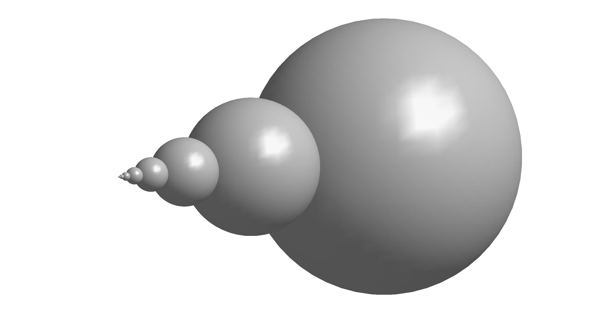
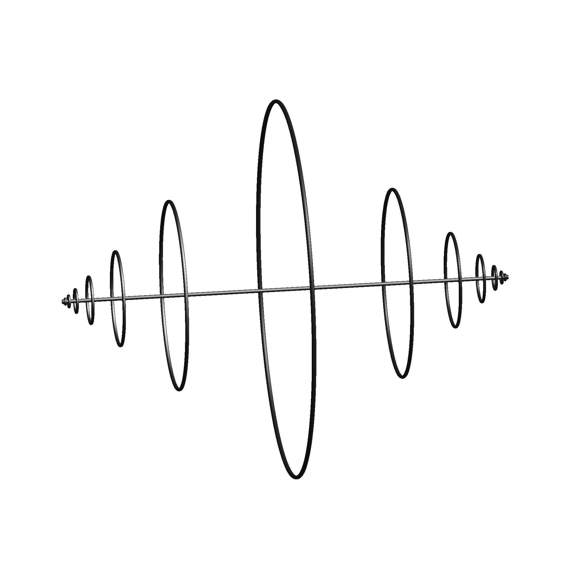
Figure 1: Left: a union of countably many spheres is in $\mathscr{F}(2)\cap\mathscr{A}(\delta)$. Right: a set in $\mathscr{F}(1)\setminus\mathscr{A}(\delta)$.

A slightly different class $\mathscr{A}(\delta)$ of admissible sets was used by the second and third author in [29]. Roughly speaking, the elements of $\mathscr{A}(\delta)$ are Ahlfors regular unions of countably many continuous images of closed manifolds, and have to satisfy two more conditions: a certain degree of flatness and a related linking condition; all this holds up to a set of $\mathscr{H}^{m}$-measure zero. The class $\mathscr{A}(\delta)$ contains, for example, finite unions of $C^{1}$ embedded manifolds that intersect each other along sets of $\mathscr{H}^{m}$-measure zero (such as the stack of spheres in Figure 1), and bi-Lipschitz images of such unions, but also certain sets with cusp singularities. For example, an arc with two tangent segments,

$$A=\big{\{}x\in{\mathbb{R}}^{2}\colon x_{1},x_{2}\geq 0\text{ and }\big{(}x_{1}^{2}+x_{2}^{2}=1\text{ or }\max_{i=1,2}|x_{i}|=1\big{)}\big{\}}$$

is in $\mathscr{A}(\delta)$ for each $\delta>0$. However, $A$ is not in $\mathscr{F}(1)$ as the $\beta_{A}(\cdot,r)$ goes to zero as $r\to 0$ at the cusp points while $\theta_{A}(x,r)$ remains constant there. On the other hand, the union of a segment and countably many circles that are contained in planes perpendicular to that segment,

$$\big{\{}(t,0,0)\colon t\in[0,1]\big{\}}\cup\bigcup_{j=1}^{\infty}\gamma_{j}\cup\bigcup_{j=2}^{\infty}\tilde{\gamma}_{j},$$

where

$$\gamma_{j}=\big{\{}2^{-j}(1,\cos\varphi,\sin\varphi)\colon\varphi\in[0,2\pi]\big{\}}$$

and $\tilde{\gamma}_{j}$ is the image of $\gamma_{j}$ under the reflection $(x,y,z)\mapsto(1-x,y,z)$, is not in $\mathscr{A}(\delta)$ as the linking condition is violated at all the points of the segment but it does belong to $\mathscr{F}(1)$, as the circles prevent the $\beta(x,r)$ from going to zero at the endpoints of the segment.

Both $\mathscr{F}(m)$ and $\mathscr{A}(\delta)$ contain sets of fractal dimension, e.g. sufficiently flat von Koch snowflakes. However, if one of our curvature energies of $\Sigma$ is finite, it follows rather easily that the Hausdorff dimension of $\Sigma$ must be $m$.

Definition 1.2 (Global Menger curvature at a point).

Let $\Sigma\in\mathcal{F}(m)$ and $x\in\Sigma$. Set

$$\mathcal{K}_{G}[\Sigma](x)\equiv\mathcal{K}_{G}(x):=\sup_{x_{1},\ldots,x_{m+1}\in\Sigma}K(x,x_{1},\ldots,x_{m+1})\,,$$

where

$$K(x,x_{1},\ldots,x_{m+1}):=\frac{\mathscr{H}^{m+1}(\operatorname{conv}(x,x_{1},\ldots,x_{m+1}))}{\mathop{\rm diam}\nolimits\bigl{(}\{x,x_{1},\ldots,x_{m+1}\}\bigr{)}^{m+2}},$$ (1.4)

and $\operatorname{conv}(E)$ and $\mathop{\rm diam}\nolimits(E)$ denote the convex hull and the diameter of a set $E$, respectively. We say that $\mathcal{K}_{G}(x)$ is the global Menger curvature of  $\Sigma$  at $x$.

When $m=1$ and $\Sigma$ is just a curve or a more general one-dimensional set  then $K(x_{0},x_{1},x_{2})$ is the ratio of the area of the triangle $T=\operatorname{conv}(x_{0},x_{1},x_{2})$ to the third power of the maximal edge length of $T$. Thus, $K$ is controlled by $R(T)^{-1}$, where $R(T)$ is the circumradius of $T$;

$$K(x_{0},x_{1},x_{2})\leq\frac{1}{4R(T)}=\frac{\text{Area}\,(T)}{|x_{0}-x_{1}|\,|x_{1}-x_{2}|\,|x_{2}-x_{0}|}\,.$$

For triangles with angles bounded away from $0$ and $\pi$, both quantities are in fact comparable. Therefore, in this case our global curvature function $\mathcal{K}_{G}$ does not exceed a constant multiple of the global curvature as defined by O. Gonzalez and J.H. Maddocks [12], and widely used afterwards; see e.g. [13], [4], [22], [21], [23], [27], [10], [9], and for global curvature on surfaces [25], [26]. Also for $m=2$, integrated powers of a function quite similar to $K(x_{0},x_{1},x_{2})$ in (1.4) were used in [28] to prove geometric variants of Morrey-Sobolev imbedding theorems for compact two-dimensional sets in ${\mathbb{R}}^{3}$ in an admissibility class slightly more general than the class $\mathscr{A}(\delta)$ defined in [29].

To define the second integrand, we first introduce the tangent-point radius, which for the purposes of this paper is a function

$$R_{\rm tp}\colon\Sigma\times\Sigma\times G(n,m)\to[0,+\infty]$$

given by

$$R_{\rm tp}(x,y;H):=\frac{|y-x|^{2}}{2\mathop{\rm dist}\nolimits(y,x+H)}\,.$$ (1.5)

Geometrically, this is the radius of the smallest sphere tangent to the affine $m$-plane $x+H$ and passing through $x$ and $y$. (If $y$ happens to be contained in $x+H$, in particular if $y=x$, then we set $1/R_{\rm tp}(x,y;H)=0$.)

Definition 1.3 (Global tangent-point curvature).

Assume that $H\colon\Sigma\to G(n,m)$ is an arbitrary map. Set

$$\mathcal{K}_{\textnormal{tp}}[\Sigma](x)\equiv\mathcal{K}_{\textnormal{tp}}(x)\equiv\mathcal{K}_{\textnormal{tp}}(x,H(x)):=\sup_{y\in\Sigma}\frac{1}{R_{\rm tp}(x,y;H(x))}\,.$$

Of course, the definition of $\mathcal{K}_{\textnormal{tp}}\colon\Sigma\to[0,+\infty]$ depends on the choice of $H$. However, we shall often omit the particular map $H$ from the notation, assuming tacitly that a choice of ‘tangent’ planes $\Sigma\ni x\mapsto H(x)\in G(n,m)$ has been fixed.

Theorem 1.4.

Let $0<m<n$ and $\Sigma\in\mathcal{F}(m)$. Assume $p>m$. The following conditions are equivalent:

1. $\Sigma$ is an embedded $W^{2,p}$-submanifold of ${\mathbb{R}}^{n}$ without boundary;

2. $\mathcal{K}_{G}[\Sigma]\in L^{p}(\Sigma,\mathscr{H}^{m})$;

3. There is a map $H\colon\Sigma\to G(n,m)$ such that for this map

   $$\mathcal{K}_{\textnormal{tp}}[\Sigma]\equiv\mathcal{K}_{\textnormal{tp}}(\cdot,H(\cdot))\ \in\ L^{p}(\Sigma,\mathscr{H}^{m}).$$

A quick comment on the equivalence of (1) and (3) should be made right away: it is a relatively simple exercise to see that for a $C^{1}$ embedded manifold $\Sigma$ the $L^{p}$ norm of $\mathcal{K}_{\textnormal{tp}}(\cdot,H(\cdot))$ can be finite for at most one continuous map $H\colon\Sigma\to G(n,m)$ – the one sending every $x\in\Sigma$ to $T_{x}\Sigma\in G(n,m)$.

Let us also mention a toy case of the equivalence of conditions (1) and (2) in the above theorem. For rectifiable curves $\gamma$ in ${\mathbb{R}}^{n}$ the equivalence of the arc-length parametrization $\Gamma$ of $\gamma$ being injective and in $W^{2,p}$, and the global curvature of $\gamma$ being in $L^{p}$ has been proved by the second and third author in [27]. To be more precise, let $S_{L}:={\mathbb{R}}/L{\mathbb{Z}},$ $L>0$, be the circle with perimeter $L$, and denote by $\Gamma:S_{L}\to{\mathbb{R}}^{n}$ the arclength parametrization of a closed rectifiable curve $\gamma:{\mathbb{S}}^{1}\to{\mathbb{R}}^{n}$ of length $L$. Then the global radius of curvature function $\rho_{G}[\gamma]:S_{L}\to{\mathbb{R}}$, ; see, e.g., [13], is defined as

$$\rho_{G}[\gamma](s):=\inf_{\sigma,\tau\in S_{L}\setminus\{s\}\atop\sigma\not=\tau}R(\Gamma(s),\Gamma(\sigma),\Gamma(\tau)),\qquad s\in S_{L}$$ (1.6)

where, again, $R(\cdot,\cdot,\cdot)$ denotes the circumradius of a triangle, and the global curvature $\kappa_{G}[\gamma](s)$ of $\gamma$ is given by

$$\kappa_{G}[\gamma](s):=\frac{1}{\rho_{G}[\gamma](s)}\,.$$ (1.7)

In [27] we prove for $p>1$ that $\Gamma\in W^{2,p}(S_{L},{\mathbb{R}}^{n})$ and $\Gamma$ is injective (so that $\gamma$ is simple) if and only if $\kappa_{G}[\gamma]\in L^{p}$. Examples show that this fails for $p=1=\dim\gamma$: There are embedded curves of class $W^{2,1}$ whose global curvature $\kappa_{G}$ is not in $L^{1}.$ The first part of the proof (3) $\Rightarrow$ (1) for $m=1$, namely the optimal $C^{1,\tau}$-regularity of curves with finite energy, is modelled on the argument that was used in [30] for a different geometric curvature energy, namely for $\iint_{\gamma\times\gamma}1/R_{\rm tp}^{q}$.

We conjecture that the implications (1) $\Rightarrow$ (2), (3) of Theorem 1.4 fail for $p=m>1$.

Remark.

If (2) or (3) holds, then according to Theorem 1.4 $\Sigma$ is embedded and locally, for some $R>0$, $\Sigma\cap\mathbb{B}^{n}(x,R)$ is congruent to a graph of a $W^{2,p}$ function $f\colon{\mathbb{R}}^{m}\to{\mathbb{R}}^{n-m}$. Since $p>m$, we also know from a result of A. Calderón and A. Zygmund (see e.g. [7, Theorem 1, p. 235]) that $Df\colon{\mathbb{R}}^{m}\to L({\mathbb{R}}^{m},{\mathbb{R}}^{n-m})$ is differentiable a.e. in the classic sense.

Remark.

One can complement Theorem 1.4 by the contribution of S. Blatt and the first author [3] in the following way. Suppose that $2\leq k\leq m+2$ and in Definition 1.2 one takes the supremum only with respect to $(m+2)-k$ points of $\Sigma$, defining the respective curvature $\mathcal{K}_{G,k}$ as a function of $k$-tuples $(x_{0},x_{1},\ldots,x_{k-1})\in\Sigma^{k}$. Suppose that $p>m(k-1)$ and $\Sigma$ is a $C^{1}$ embedded manifold. Then, $\mathcal{K}_{G,k}$ is of class $L^{p}(\Sigma^{k},\mathscr{H}^{mk})$ if and only if $\Sigma$ is locally a graph of class $W^{1+s,p}({\mathbb{R}}^{m},{\mathbb{R}}^{n-m})$, where $s=1-m(k-1)p^{-1}\in(0,1)$. If $k=m+2$ and $p>m(m+2)$, then the assumption that $\Sigma$ be a $C^{1}$ manifold is not necessary; one can just assume $\Sigma\in\mathscr{F}(m)$. See [3] for details. We believe that the characterization of [3] does hold for all $2\leq k\leq m+2$ without the assumption that $\Sigma$ is of class $C^{1}$. (To prove this, one would have to generalize the regularity theory presented in [16] to all curvatures $\mathcal{K}_{G,k}$).

Blatt’s preprint [2] contains a similar characterization in terms of fractional Sobolev spaces of those $C^{1}$ manifolds $\Sigma$ for which the tangent–point energy $\iint_{\Sigma\times\Sigma}1/(R_{\rm tp})^{q}$ is finite.

Remark.

W. Allard, in his classic paper [1], develops a regularity theory for $m$-dimensional varifolds whose first variation (i.e., the distributional counterpart of mean curvature) is in $L^{p}$ for some $p>m$. His Theorem 8.1 ascertains that, under mild extra assumptions on the density function of such a varifold $V$, an open and dense subset of the support of $\|V\|$ is locally a graph of class $C^{1,1-m/p}$. For $p>m$ Sobolev–Morrey imbedding yields $W^{2,p}\subset C^{1,1-m/p}$ and one might naïvely wonder if a stronger theorem does hold, implying Allard’s (qualitative) conclusion just by Sobolev–Morrey. Indeed, J.P. Duggan [6] proved later an optimal result in this direction. For integral varifolds, $W^{2,p}$-regularity can be obtained directly via elliptic regularity theory, see U. Menne [19, Lemmata 3.6 and 3.21].

In Allard’s case the ‘lack of holes’ is built into his assumption on the first variation $\delta V$ of $V$. Our setting is not so close to PDE theory: both ‘curvatures’ are defined in purely geometric terms and in a nonlocal way. Here, the ‘lack of holes’ follows, roughly speaking, from a delicate interplay between the inequality $\theta(x,r)\lesssim\beta(x,r)$ built into the definition of $\mathscr{F}(m)$ and the decay of $\beta(x,r)$ which follows from the finiteness of energy. A more detailed account on our strategy of proof here, is presented in the next subsection.

At this stage we do not know for our curvature energies what the situation is like in the scale invariant case $p=m$. For two-dimensional integer multiplicity varifolds, however (or in the simpler situation of $W^{2,2}$-graphs over planar domains) Toro [31] was able to prove the existence of bi-Lipschitz parametrizations. For $m$-dimensional sets Toro [32, eq. (1)] established a sufficient condition for the existence of bi-Lipschitz parametrizations in terms of $\theta$. Her condition is satisfied, e.g., by S. Semmes’ chord-arc surfaces with small constant, and by graphs of functions that are sufficiently well approximated by affine functions; see [32, Section 5] for the details.

Remark.

Following the reasoning in [27, Lemma 7] one can easily provide nontrivial lower bounds for the global tangent-point curvature for hypersurfaces ($n=m+1$), and also for curves $m=1<n$; see Theorem 1.5 below. Indeed, setting $E:=\|\mathcal{K}_{\textnormal{tp}}[\Sigma]\|_{L^{p}(\Sigma)}$, where $\Sigma\subset{\mathbb{R}}^{n}$ is a compact connected $m$-dimensional $C^{1}$-submanifold without boundary, we can find at least one point $x\in\Sigma$ such that $\mathcal{K}_{\textnormal{tp}}[\Sigma](x)\leq E/(\mathscr{H}^{m}(\Sigma)^{1/p}),$ since otherwise we had a contradiction via

$$E=\left(\int_{\Sigma}\Big{(}\mathcal{K}_{\textnormal{tp}}[\Sigma](x)\Big{)}^{p}\,d\mathscr{H}^{m}(x)\right)^{1/p}>\frac{E}{\mathscr{H^{m}}(\Sigma)^{1/p}}\mathscr{H^{m}}(\Sigma)^{1/p}=E.$$

Therefore $R:=\inf_{y\in\Sigma}R_{\textnormal{tp}}(x,y,T_{x}\Sigma)\geq\mathscr{H}^{m}(\Sigma)^{1/p}/E.$ If there existed an open ball $\mathbb{B}^{n}(a,R)$ with

$$(x+T_{x}\Sigma)\cap\partial\mathbb{B}^{n}(a,R)=\{x\}$$

such that $\Sigma\cap\mathbb{B}^{n}(a,R)\not=\emptyset$, then we could find a strictly smaller sphere tangent to $\Sigma$ in $x$ and containing yet another point $y\in\Sigma$ contradicting the definition of $R$. Hence we have shown that the union of such open balls

$$M:=\bigcup\{\mathbb{B}^{n}(a,R):\partial\mathbb{B}^{n}(a,R)\cap(x+T_{x}\Sigma)=\{x\}\}$$ (1.8)

contains no point of $\Sigma.$ In other words, $\Sigma$ is a compact embedded submanifold without boundary, contained in ${\mathbb{R}}^{n}\setminus M$, and one can ask for the area minimizing submanifold in ${\mathbb{R}}^{n}\setminus M$. In codimension one, i.e., for $m=n-1$, $\Sigma=\partial\Omega$ for a bounded open set $\Omega\subset{\mathbb{R}}^{n}$, and the union of balls defining $M$ just consists of two such balls, one in $\Omega$ and one in the unbounded exterior of $\Sigma$. So, due to the classic isoperimetric inequality (see, e.g. [8, Theorem 3.2.43]) one finds

$$\mathscr{H}^{n-1}(\Sigma) \geq n\omega_{n}^{1/n}\mathscr{H}^{n}((\Omega))^{\frac{n-1}{n}}$$

$$\geq n\omega_{n}^{1/n}\mathscr{H}^{n}(B(a,R))^{\frac{n-1}{n}}=\mathscr{H}^{n-1}(\partial\mathbb{B}^{n}(a,R))=n\omega_{n}R^{n-1}.$$

which by definition of $R$ can be rewritten as

$$\|\mathcal{K}_{\textnormal{tp}}[\Sigma]\|_{L^{p}(\Sigma)}=E\geq(\mathscr{H}^{n-1}(\Sigma))^{\frac{1}{p}-\frac{1}{n-1}}(n\omega_{n})^{\frac{1}{n-1}}$$ (1.9)

with equality if and only if $\Sigma$ equals a round sphere. Hence, we obtain the following simple result.

Theorem 1.5.

Let $p>0$. Among all compact embedded $C^{1}$-hypersurfaces with given surface area, the round sphere uniquely (up to isometries) minimizes the energy $\|\mathcal{K}_{\textnormal{tp}}[\Sigma]\|_{L^{p}(\Sigma,\mathscr{H}^{n-1})}.$ If $p>n-1$, the same holds true for all $(n-1)$-fine sets $\Sigma\in\mathscr{F}(n-1)$.

Similarly, for $m=1$ one concludes that any of those great circles on any of the balls $\mathbb{B}^{n}(a,R)$ generating $M$ in (1.8) that are also geodesics on $M$ uniquely minimize $E$ among all closed simple $C^{1}$-curves $\Sigma\equiv\gamma\subset{\mathbb{R}}^{n}\setminus M$, which provides the lower bound

$$\|\mathcal{K}_{\textnormal{tp}}[\gamma]\|_{L^{p}(\gamma)}=E\geq 2\pi\mathscr{H}^{1}(\gamma)^{\frac{1}{p}-1}.$$ (1.10)

This is exactly what we found for curves in [27, Lemma 7 (3.1)], and is also consistent with (1.9) if $n=2=m+1$.

1.2 Essential ideas and an outline of the proof.

This paper grew out of our interest in geometric curvature energies and earlier related research, cf. [27], [24], [28], [29] and [16]. While working on the integral Menger curvature energy of rectifiable curves $\gamma\subset{\mathbb{R}}^{n}$

$$\mathscr{M}_{p}(\gamma)=\iiint_{\gamma\times\gamma\times\gamma}\frac{1}{R^{p}(x,y,z)}\,d\mathscr{H}^{1}(x)\,d\mathscr{H}^{1}(y)\,d\mathscr{H}^{1}(z)\,,\qquad p>3,$$

we realized how slicing can be used to obtain optimal Hölder continuity of arc-length parametrizations. (The scale invariant exponent $p=3$ is critical here: polygons have infinite $M_{p}$-energy precisely for $p\geq 3$; see S. Scholtes [20] for a proof).

One crucial difference between curves $\gamma$ and $m$-dimensional sets $\Sigma$ in ${\mathbb{R}}^{n}$ for $m\geq 2$ lies in the distribution of mass in balls on various scales: If $\gamma$ is a rectifiable curve and $r<\frac{1}{2}\mathop{\rm diam}\nolimits\gamma$, then obviously $\mathscr{H}^{1}(\gamma\cap\mathbb{B}^{n}(x,r))\geq r$ for each $x\in\gamma$. For $m>1$ the measure $\mathscr{H}^{m}(\Sigma\cap\mathbb{B}^{n}(x,r))$ might be much smaller than $r^{m}$ due to complicated geometry of $\Sigma$ at intermediate length scales. In [28] we have devised a method, allowing us to obtain estimates of $\mathscr{H}^{m}(\Sigma\cap\mathbb{B}^{n}(x,r))$ for $m=2$, $n=3$ and all radii $r<R_{0}$, with $R_{0}$ depending only on the energy level of $\Sigma$ in terms of its integral Menger curvature. This method has been later reworked and extended in the subsequent papers [29], [16], to yield the so-called uniform Ahlfors regularity, i.e., estimates of the form

$$\mathscr{H}^{m}(\Sigma\cap\mathbb{B}^{n}(x,r))\geq\frac{1}{2}\omega_{m}r^{m},\qquad\,\,\,\text{for all }\,\,r<R_{0}=R_{0}(\text{energy})\,,$$

for other curvature energies and arbitrary $0<m<n$ (to cope with the case of higher codimension, we used a linking invariant to guarantee that $\Sigma$ has large projections onto some $m$-dimensional planes). Combining such estimates for $\mathscr{H}^{m}(\Sigma\cap\mathbb{B}^{n}(x,r))$ with an extension of ideas from [24] we obtained in [28], [29] and [16] a series of results, establishing $C^{1,\alpha}$ regularity for surfaces, or more generally, for a priori non-smooth $m$-dimensional sets for which certain geometric curvature energies are finite. Finally, we also realized that the well-known pointwise characterization of $W^{1,p}$-spaces of P. Hajłasz [14] is the missing link, allowing us to combine the ideas from [16] and [29] in the present paper in order to provide with Theorem 1.4 a far-reaching, general extension of [27, Theorems 1 & 2] from curves to $m$-dimensional manifolds in ${\mathbb{R}}^{n}$.

Let us now discuss the plan of proof of Theorem 1.4 and outline the structure of the whole paper.

The easier part is to check that if $\Sigma$ is an embedded compact $W^{2,p}$ manifold without boundary, then conditions (2) and (3) hold. We work in small balls $\mathbb{B}(x,R)$ centered on $\Sigma$, with $R>0$ chosen so that $\Sigma\cap\mathbb{B}(x,R)$ is a (very flat) graph of a $W^{2,p}$ function $f\colon\mathbb{B}^{m}(x,2R)\to{\mathbb{R}}^{n-m}$. Using Morrey’s inequality twice, we first show that

$$\beta_{\Sigma}(a,r)\lesssim g(a)r,\qquad a\in\mathbb{B}(x,R)\cap\Sigma,\quad 0<r<R\,,$$

for a function $g\in L^{p}$ that is comparable to some maximal function of $|D^{2}f|$. Next, working with this estimate of beta numbers on all scales $r=R/2^{k}$, $k=0,1,2,\ldots$, we show that in each coordinate patch each of the global curvatures $\mathcal{K}_{G}$ and $\mathcal{K}_{\textnormal{tp}}$ can be controlled by two terms,

$$\mathcal{K}_{G}(a),\text{resp. }\mathcal{K}_{\textnormal{tp}}(a)\lesssim g(a)+C(R)\,$$

where $C(R)$ is a harmless term depending only on the size of the patches. (It is clear from the definitions that for embedded manifolds one can estimate both $\mathcal{K}_{G}$ and $\mathcal{K}_{\textnormal{tp}}$ taking into account only the local bending of $\Sigma$ and working in coordinate patches of fixed size; the effects of self-intersections are not an issue). This yields $L^{p}$-integrability of $\mathcal{K}_{G}$ and $\mathcal{K}_{\textnormal{tp}}$. We refer to Section 4 for the details.

The reverse implications require more work. The proofs that (3) or (2) implies (1) have, roughly speaking, four separate stages. First, we use energy estimates to show that if $\|\mathcal{K}_{G}\|_{L^{p}}$ or $\|\mathcal{K}_{\textnormal{tp}}\|_{L^{p}}$ are less than $E^{1/p}$ for some finite constant $E$, then

$$\beta_{\Sigma}(x,r)\lesssim\left(\frac{E}{A_{\Sigma}}\right)^{\kappa/(p-m)}r^{\kappa}\,.$$

Here $\kappa$ denotes a number in $(0,1-m/p)$, depending only on $m,p$ with different explicit values for $\mathcal{K}_{G}$ or $\mathcal{K}_{\textnormal{tp}}$, and $A_{\Sigma}$ is the constant from Definition 1.1 measuring Ahlfors regularity of $\Sigma$. By the very definition of $m$-fine sets, such an estimate implies that the bilateral beta numbers of $\Sigma$ tend to zero with a speed controlled by $r^{\kappa}$. In particular, $\Sigma$ is Reifenberg flat with vanishing constant, and an application of [5, Proposition 9.1] shows that $\Sigma$ is an embedded manifold of class $C^{1,\kappa}$. See Section 3.1 for more details.

Next, we prove the uniform Ahlfors regularity of $\Sigma$, i.e. we show that

$$\mathscr{H}^{m}(\Sigma\cap\mathbb{B}(x,r))\geq\frac{1}{2}\mathscr{H}^{m}(\mathbb{B}^{m}(x,r))$$

for all radii $r\in(0,R_{0})$, where $R_{0}$ depends only on the energy bound $E$ and the parameters $n,m,p$, but not at all on $\Sigma$ itself. Here, we rely on methods from our previous papers [16] and [28, 29]. Roughly speaking, we combine topological arguments based on the linking invariant with energy estimates to show that for each $r<R_{0}=R_{0}(E,n,m,p)$ the portion of $\Sigma$ in $\mathbb{B}^{n}(x,r)$ has large projection onto some plane $H=H(r)\in G(n,m)$. See Section 3.2.

(There is a certain freedom in this phase of the proof; it would be possible to prove uniform Ahlfors regularity first, and estimate the decay of $\beta_{\Sigma}(x,r)$ afterwards. This approach has been used in [28, 29].)

After the second step we know that in coordinate patches of diameter comparable to $R_{0}$ the manifold $\Sigma$ coincides with a graph of a function $f\in C^{1,\kappa}(\mathbb{B}^{m},{\mathbb{R}}^{n-m})$. The third stage is to bootstrap the Hölder exponent $\kappa$ to the optimal $\tau=1-m/p>\kappa$ for both global curvatures $\mathcal{K}_{G}$ and $\mathcal{K}_{\textnormal{tp}}$. This is achieved by an iterative argument which uses slicing: If the integral of the global curvature to the power $p$ over a ball is not too large, then this global curvature itself cannot be too large on a substantial set of good points in that ball. Geometric arguments based on the definition of the global curvature functions $\mathcal{K}_{G}$ and $\mathcal{K}_{\textnormal{tp}}$ show that $|Df(x)-Df(y)|\lesssim|x-y|^{\tau}$ on the set of good points. It turns out that there are plenty of good points at all scales, and in the limit we obtain a similar Hölder estimate on the whole domain of $f$. See Section 3.3.

The fourth and last step is to combine the $C^{1,\tau}$-estimates with a pointwise characterization of first order Sobolev spaces obtained by Hajłasz [14]. The idea is very simple. Namely, the bootstrap reasoning in the third stage of the proof (Section 3.3) yields the following, e.g. for the global Menger curvature $\mathcal{K}_{G}$: On a scale $R_{1}\approx R_{0}$, the intersection $\Sigma\cap\mathbb{B}^{n}(a,R_{1})$ coincides with a flat graph of a function $f\colon P\simeq{\mathbb{R}}^{m}\to{\mathbb{R}}^{n-m}\simeq P^{\perp}$, with

$$|Df(x)-Df(y)|\lesssim\biggl{(}\int_{\mathbb{B}^{m}(\frac{x+y}{2},5|x-y|)}\mathcal{K}_{G}\bigl{(}(\xi,f(\xi))\bigr{)}^{p}\,d\xi\biggr{)}^{1/p}|x-y|^{\tau}\,$$

for $\tau=1-m/p$. Such an inequality is true for every $p>m$ so we can easily fix a number $p^{\prime}\in(m,p)$ and show that

$$|Df(x)-Df(y)|\lesssim\bigl{(}M(x)+M(y)\bigr{)}|x-y|\,,$$ (1.11)

where $M(\cdot)^{p^{\prime}}$ is the Hardy–Littlewood maximal function of the global curvature. Since $p/p^{\prime}>1$, an application of the Hardy–Littlewood maximal theorem yields $M^{p^{\prime}}\in L^{p/p^{\prime}}$, or, equivalently, $M\in L^{p}$. Thus, by the well known result of Hajłasz (see Section 2.3), (1.11) implies that $Df\in W^{1,p}$. In fact, the $L^{p}$ norm of $D^{2}f$ is controlled by a constant times the $L^{p}$-norm of the global Menger curvature $\mathcal{K}_{G}$. An analogous argument works for the global tangent-point curvature function $\mathcal{K}_{\textnormal{tp}}$. This concludes the whole proof; see Section 3.4.

For each of the global curvatures $\mathcal{K}^{(i)}_{G}$, there are some technical variations in that scheme; here and there we need to adjust an argument to one of them. However, the overall plan is the same in both cases.

The paper is organized as follows. In Section 2, we gather some preliminaries from linear algebra and some elementary facts about simplices, introduce some specific notation, and list some auxiliary results with references to existing literature. Section 3 forms the bulk of the paper. Here, following the sketch given above, we prove that $L^{p}$ bounds for (either of) the global curvatures imply that $\Sigma$ is an embedded manifold with local graph representations of class $W^{2,p}$. Finally, in Section 4 we prove the reverse implications, concluding the whole proof of Theorem 1.4.

Acknowledgement. The authors are grateful to the anonymous referee for her/his careful reading of this paper and the suggestions which have helped to improve the presentation of our work.

2 Preliminaries

2.1 The Grassmannian

In this paragraph we gather a few elementary facts about the angular metric $\operatorname{\varangle}(\cdot,\cdot)$ on the Grassmannian $G(n,m)$ of $m$-dimensional linear subspaces of ${\mathbb{R}}^{n}$.

Here is a summary: for two $m$-dimensional linear subspaces

$$U=\mathrm{span}\,\{u_{1},\ldots,u_{m}\}\qquad\text{and}\qquad V=\mathrm{span}\,\{v_{1},\ldots,v_{m}\}$$

in ${\mathbb{R}}^{n}$ such that the bases $(u_{1},\ldots,u_{m})$, $(v_{1},\ldots,v_{m})$ are roughly orthonormal and such that $|u_{i}-v_{i}|\leq\varepsilon$, we have the estimate $\operatorname{\varangle}(U,V)\lesssim\varepsilon$. This will become especially useful in Section 3.3.

For $U\in G(n,m)$ we write $\pi_{U}$ to denote the orthogonal projection of ${\mathbb{R}}^{n}$ onto $U$ and we set $Q_{U}={{\rm Id}}_{{\mathbb{R}}^{n}}-\pi_{U}=\pi_{U^{\perp}}$, where ${{\rm Id}}_{{\mathbb{R}}^{n}}:{\mathbb{R}}^{n}\to{\mathbb{R}}^{n}$ denotes the identity mapping.

Definition 2.1.

Let $U,V\in G(n,m)$. We set

$$\operatorname{\varangle}(U,V):=\|\pi_{U}-\pi_{V}\|=\sup_{w\in{\mathbb{S}}^{n-1}}|\pi_{U}(w)-\pi_{V}(w)|\,.$$

The function $\operatorname{\varangle}(\cdot,\cdot)$ defines a metric on the Grassmannian $G(n,m)$. The topology induced by this metric agrees with the standard quotient topology of $G(n,m)$. We list several properties of $\operatorname{\varangle}$ below. They will become useful for Hölder estimates of the graph parameterizations of $\Sigma$ in Section 3.3. The proofs are elementary and we omit them here.

Remark.

Notice that

$$\operatorname{\varangle}(U,V)=\|\pi_{U}-\pi_{V}\|=\|{{\rm Id}}_{{\mathbb{R}}^{n}}-Q_{U}-({{\rm Id}}_{{\mathbb{R}}^{n}}-Q_{V})\|=\|Q_{V}-Q_{U}\|\,.$$

Proposition 2.2 (Lemma 2.2 in [29]).

If the spaces $U,V\in G(n,m)$ have orthonormal bases $(e_{1},\ldots,e_{m})$ and $(f_{1},\ldots,f_{m})$, respectively, and if $|e_{i}-f_{i}|\leq\vartheta$ for $i=1,\ldots,m$, then $\operatorname{\varangle}(U,V)\leq 2m\vartheta$.

Definition 2.3.

Let $V\in G(n,m)$ and let $(v_{1},\ldots,v_{m})$ be a basis of $V$. Fix some radius $\rho>0$ and two constants $\varepsilon\in(0,1)$ and $\delta\in(0,1)$. We say that $(v_{1},\ldots,v_{m})$ is a $(\rho,\varepsilon,\delta)$-basis if

$$(1-\varepsilon)\rho\leq|v_{i}| \leq(1+\varepsilon)\rho\quad\text{for }i=1,\ldots,m$$

$$\text{and}\quad|\langle v_{i},v_{j}\rangle| \leq\delta\rho^{2}\quad\text{for }i\neq j\,.$$

Specifically, a $(\rho,0,0)$-basis will be called ortho-$\rho$-normal.

Proposition 2.4.

Let $\rho>0$, $\varepsilon\in(0,1/2)$ and $\delta\in(0,1)$ be some constants. Let $(v_{1},\ldots,v_{m})$ be a $(\rho,\varepsilon,\delta)$-basis of $V\in G(n,m)$. Then there exist an ortho-$\rho$-normal-basis $(\hat{v}_{1},\ldots,\hat{v}_{m})$ of $V$ and a constant $C_{2}=C_{2}(m)$ such that

$$|v_{i}-\hat{v}_{i}|\leq(\varepsilon+C_{2}\delta)\rho\quad\text{for }i=1,\ldots,m\,.$$

Proof.

By scaling we may assume that $\rho=1$. Define $w_{i}:=v_{i}/|v_{i}|$ for $i=1,\ldots,m$, $f_{1}:=w_{1}$, $\hat{v}_{1}:=w_{1},$ and then recursively

$$f_{k}:=w_{k}-\sum_{i=1}^{k-1}\langle w_{k},\hat{v}_{i}\rangle\hat{v}_{i},\qquad\textnormal{and}\quad\hat{v}_{k}:=f_{k}/|f_{k}|\quad\textnormal{ for $k=1,\ldots,m$},$$

and observe that $|w_{i}-v_{i}|=|1-|v_{i}||\leq\epsilon$ and $|\langle w_{i},w_{j}\rangle|\leq\delta/(1-\epsilon)^{2}<4\delta$ for all $i,j=1,\ldots,m$, and in addition, $V=\mathop{\rm span}\nolimits\{w_{1},\ldots,w_{m}\}=\mathop{\rm span}\nolimits\{\hat{v}_{1},\ldots,\hat{v}_{m}\}$ by construction. Notice that $||f_{k}|-1|=||f_{k}|-|w_{k}||\leq|f_{k}-w_{k}|$, and therefore

$$|f_{k}-\hat{v}_{k}|=||f_{k}|-1|\leq|f_{k}-w_{k}|$$

so that by

$$|v_{k}-\hat{v}_{k}|\leq|v_{k}-w_{k}|+|w_{k}-f_{k}|+|f_{k}-\hat{v}_{k}|\leq\epsilon+2|f_{k}-w_{k}|$$

the main task turns out to be to estimate $a_{k}:=|f_{k}-w_{k}|$ for $k=1,\ldots,m$, where we get immediately $a_{1}=0$ by definition. If one estimates

$$a_{k} \leq\sum_{i=1}^{k-1}|\langle w_{k},w_{i}\rangle|+\sum_{i=1}^{k-1}|w_{i}-\hat{v}_{i}|$$

$$\leq 4\delta(k-1)+\sum_{i=1}^{k-1}(a_{i}+|f_{i}-\hat{v}_{i}|)$$

$$\leq 4\delta(k-1)+2\sum_{i=1}^{k-1}a_{i},$$

one can prove by induction that

$$a_{k}\leq 4\delta\Big{[}(k-1)+2\sum_{i=0}^{l}3^{i}(k-i-2)\Big{]}+2\cdot 3^{l+1}\sum_{i=1}^{k-l-2}a_{i}\quad\text{for all }l=0,\ldots,k-3.$$

Specifically for $l=k-3$ we obtain

$$a_{k}\leq 4\delta\Big{[}(k-1)+2\sum_{i=0}^{k-3}3^{i}(k-i-2)\Big{]},$$

and therefore, for all $k=1,\ldots,m,$

$$|v_{k}-\hat{v}_{k}|\leq\varepsilon+8\delta\Big{[}(m-1)+2\sum_{i=0}^{m-3}3^{i}(m-i-2)\Big{]}=:\varepsilon+C_{2}(m)\delta\,.\qed$$

Proposition 2.5.

Let $U,V\in G(n,m)$ and let $(e_{1},\ldots,e_{m})$ be some orthonormal basis of $V$. Assume that for each $i=1,\ldots,m$ we have the estimate $\mathop{\rm dist}\nolimits(e_{i},U)=|Q_{U}(e_{i})|\leq\vartheta$ for some $\vartheta\in(0,1/\sqrt{2})$. Then there exists a constant $C_{3}=C_{3}(m)$ such that

$$\operatorname{\varangle}(U,V)\leq C_{3}\vartheta\,.$$

Proof.

Set $u_{i}:=\pi_{U}(e_{i})$. For each $i=1,\ldots,m$ we have $|Q_{U}(e_{i})|\leq\vartheta$, so

$$|u_{i}-e_{i}| =|Q_{U}(e_{i})|\leq\vartheta\quad\text{hence}$$

$$1-\vartheta^{2}<\sqrt{1-\vartheta^{2}} \leq|u_{i}|\leq 1<1+\vartheta^{2}\quad\text{for }i=1,\ldots,m\,.$$ (2.12)

For any $i\neq j$ the vectors $e_{i}$ and $e_{j}$ are orthogonal, hence

$$0=\langle e_{i},e_{j}\rangle =\langle\pi_{U}(e_{i})+Q_{U}(e_{i}),\pi_{U}(e_{j})+Q_{U}(e_{j})\rangle$$

$$=\langle\pi_{U}(e_{i}),\pi_{U}(e_{j})\rangle+\langle Q_{U}(e_{i}),Q_{U}(e_{j})\rangle\,.$$

Therefore

$$|\langle u_{i},u_{j}\rangle|=|\langle Q_{U}(e_{i}),Q_{U}(e_{j})\rangle|\leq|Q_{U}(e_{i})||Q_{U}(e_{j})|\leq\vartheta^{2}\,.$$ (2.13)

Estimates (2.12) and (2.13) show that $(u_{1},\ldots,u_{m})$ is a $(\rho,\varepsilon,\delta)$-basis of $U$ with constants $\rho=1$, $\varepsilon=\vartheta^{2}$ and $\delta=\vartheta^{2}$. Let $(f_{1},\ldots,f_{m})$ be the orthonormal basis of $U$ arising from $(u_{1},\ldots,u_{m})$ by means of Proposition 2.4, so that we obtain

$$|f_{i}-e_{i}|\leq|f_{i}-u_{i}|+|u_{i}-e_{i}|\leq(1+C_{2})\vartheta^{2}+\vartheta\,.$$

Using Proposition 2.2 and the fact that $\vartheta^{2}<\vartheta<1$ we finally get

$$\operatorname{\varangle}(U,V)\leq 2m((1+C_{2})\vartheta^{2}+\vartheta)\leq 2m(1+C_{2}+1)\vartheta\,.$$

Now we can set $C_{3}=C_{3}(m):=2m(1+C_{2}(m)+1)=2m(2+C_{2}(m))$. ∎

Proposition 2.6.

Let $(v_{1},\ldots,v_{m})$ be a $(\rho,\varepsilon,\delta)$-basis of $V\in G(n,m)$ with constants $\rho>0$, $\varepsilon\in(0,1/2)$ and $\delta\in(0,1)$. Let $(u_{1},\ldots,u_{m})$ be some basis of $U\in G(n,m)$, such that $|u_{i}-v_{i}|\leq\vartheta\rho$ for some $\vartheta\in(0,\tfrac{1}{\sqrt{2}}-\tfrac{1}{4})$ and for each $i=1,\ldots,m$. Furthermore, let us assume that

$$C_{3}(\varepsilon+C_{2}\delta)<1/2\,.$$ (2.14)

Then there exists a constant $C_{4}=C_{4}(m,\varepsilon,\delta)$ such that

$$\operatorname{\varangle}(U,V)\leq C_{4}\vartheta\,.$$

Proof.

Set $e_{i}:=v_{i}/\rho$ and let $(\hat{e}_{1},\ldots,\hat{e}_{m})$ be the orthonormal basis of $V$ arising from $(e_{1},\ldots,e_{m})$ by virtue of Proposition 2.4. Set $f_{i}:=u_{i}/\rho$.

$$|Q_{U}(\hat{e}_{i})| \leq|Q_{U}(\hat{e}_{i}-e_{i})|+|Q_{U}(e_{i})|\leq|\hat{e}_{i}-e_{i}|\operatorname{\varangle}(U,V)+|e_{i}-f_{i}|$$

$$\leq|\hat{e}_{i}-e_{i}|\operatorname{\varangle}(U,V)+\vartheta\,.$$

From Proposition 2.4 we have $|\hat{e}_{i}-e_{i}|\leq\varepsilon+C_{2}\delta$, so

$$|Q_{U}(\hat{e}_{i})|\leq(\varepsilon+C_{2}\delta)\operatorname{\varangle}(U,V)+\vartheta\leq 2(\epsilon+C_{2}\delta)+\vartheta\overset{\eqref{cond:eps-del}}{<}\frac{1}{4}+\vartheta<\frac{1}{\sqrt{2}}\,,$$

since $C_{3}(m)\geq 4$ for all $m\in{\mathbb{N}}$; see the definition of $C_{3}(m)$ at the end of the proof of Proposition 2.5. Hence Proposition 2.5 is applicable to the orthonormal basis $(\hat{e}_{1},\ldots,\hat{e}_{m})$ of $V$, and we conclude

$$\operatorname{\varangle}(U,V)\leq C_{3}(\varepsilon+C_{2}\delta)\operatorname{\varangle}(U,V)+C_{3}\vartheta$$

$$\text{hence}\qquad(1-C_{3}(\varepsilon+C_{2}\delta))\operatorname{\varangle}(U,V)\leq C_{3}\vartheta\,.$$

Since we assumed (2.14) we can divide both sides by $1-C_{3}(\varepsilon+C_{2}\delta)$ reaching the estimate

$$\operatorname{\varangle}(U,V)\leq\frac{C_{3}}{1-C_{3}(\varepsilon+C_{2}\delta)}\vartheta\,.$$

Finally we set

$$C_{4}=C_{4}(m,\varepsilon,\delta):=\frac{C_{3}(m)}{1-C_{3}(m)(\varepsilon+C_{2}(m)\delta)}\,.\qed$$

2.2 Angles and intersections of tubes

The results of this subsection are taken from our earlier work [29]. We are concerned with the intersection of two tubes whose $m$-dimensional ‘axes’ form a small angle, i.e. with the set

$$S(H_{1},H_{2}):=\{y\in{\mathbb{R}}^{n}\,\colon\mathop{\rm dist}\nolimits(y,H_{i})\leq 1\quad\mbox{for $i=1,2$}\},$$ (2.15)

where $H_{1}\not=H_{2}\in G(n,m)$ are such that $\pi_{H_{1}}$ restricted to $H_{2}$ is bijective. Since the set $\{y\in{\mathbb{R}}^{n}\,\colon\mathop{\rm dist}\nolimits(y,H_{i})\leq 1\}$ is convex, closed and centrally symmetric for each $i=1,2$, we immediately obtain the following:

Lemma 2.7.

$S(H_{1},H_{2})$ is a convex, closed and centrally symmetric set in ${\mathbb{R}}^{n}$; $\pi_{H_{1}}(S(H_{1},H_{2}))$ is a convex, closed and centrally symmetric set in $H_{1}\cong{\mathbb{R}}^{m}$.

For the global tangent-point curvature $\mathcal{K}_{\textnormal{tp}}$, the next lemma and its corollary provide a key tool in bootstrap estimates in Section 3.3.

Lemma 2.8.

There exist constants $1>\varepsilon_{1}=\varepsilon_{1}(m)>0$ and $c_{2}(m)<\infty$ with the following property. If $H_{1},H_{2}\in G(n,m)$ satisfy $0<\mathop{\mbox{$<\!\!\!)$}}\nolimits(H_{1},H_{2})=\alpha<\varepsilon_{1}$, then there exists an $(m-1)$-dimensional subspace $W\subset H_{1}$ such that

$$\pi_{H_{1}}\bigl{(}S(H_{1},H_{2})\bigr{)}\subset\{y\in H_{1}\colon\mathop{\rm dist}\nolimits(y,W)\leq 5c_{2}/\alpha\}\,.$$

For the proof, we refer to [29, Lemma 2.6]. It is an instructive elementary exercise in classical geometry to see why this lemma is true for $m=2$ and $n=3$.

The next lemma is now practically obvious.

Lemma 2.9.

Suppose that $H\in G(n,m)$ and a set $S^{\prime}\subset H$ is contained in $\{y\in H\colon\mathop{\rm dist}\nolimits(y,W)\leq d\}$ for some $d>0$, where $W$ is an $(m-1)$-dimensional subspace of $H$. Then

$$\mathscr{H}^{m}\bigl{(}S^{\prime}\cap\mathbb{B}^{n}(a,s)\bigr{)}\leq 2^{m}s^{m-1}d\,$$

for each $a\in H$ and each $s>0$.

Proof.

Writing each $y\in S^{\prime}\cap\mathbb{B}^{n}(a,s)$ as $y=\pi_{W}(y)+(y-\pi_{W}(y))$, one sees that $S^{\prime}\cap\mathbb{B}^{n}(a,s)$ is contained in a rectangular box with $(m-1)$ edges parallel to $W$ and of length $2s$ and the remaining edge perpendicular to $W$ and of length $2d$. ∎

2.3 The voluminous simplices

Several energy estimates for the global Menger curvature are based on considerations of simplices that are roughly regular, which means that they have all edges $\approx d$ and volume $\approx d^{m+1}$. Here are the necessary definitions, making this vague description precise.

Definition 2.10.

Let $T=\operatorname{conv}(x_{0},\ldots,x_{m+1})$ be an $(m+1)$-dimensional simplex in ${\mathbb{R}}^{n}$. For each $j=0,\ldots,m+1$ we define the faces $\mathfrak{fc}_{j}(T)$, the heights $0pt_{j}(T)$ and the minimal height $\mathfrak{h}_{\text{min}}(T)$ by

$$\mathfrak{fc}_{j}(T) =\operatorname{conv}(x_{0},\ldots,x_{j-1},x_{j+1},\ldots,x_{m+1})\,,$$

$$0pt_{j}(T) =\mathop{\rm dist}\nolimits(x_{j},\operatorname{aff}\{x_{0},\ldots,x_{j-1},x_{j+1},\ldots,x_{m+1}\})$$

$$\text{and}\quad\mathfrak{h}_{\text{min}}(T) =\min\{0pt_{i}(T):i=0,1,\ldots,m+1\}\,,$$

where $\operatorname{aff}\{p_{0},\ldots,p_{N}\}$ denotes the (at most $N$-dimensional) affine plane spanned by $N+1$ the points $p_{0},\ldots,p_{N}\in{\mathbb{R}}^{n}.$

Note that for any $(m+1)$-dimensional simplex $T$ the volume is given by

$$\mathscr{H}^{m+1}(T)=\frac{1}{m+1}0pt_{i}(T)\mathscr{H}^{m}(\mathfrak{fc}_{i}(T))\quad\textnormal{for any $i\in\{0,\ldots,m+1\}.$}$$ (2.16)

The faces $\mathfrak{fc}_{i}(T)$ are lower-dimensional simplices themselves, so that a simple inductive argument yields the estimate

$$\mathscr{H}^{m+1}(T)\geq\frac{1}{(m+1)!}0pt_{\textnormal{min}}(T)^{m+1}.$$ (2.17)

Definition 2.11.

Fix some $\eta\in[0,1]$ and $d>0$. Let $T=\operatorname{conv}(x_{0},\ldots,x_{m+1})$ be an $(m+1)$-dimensional simplex in ${\mathbb{R}}^{n}$. We say that $T$ is $(\eta,d)$-voluminous and write $T\in\mathscr{V}(\eta,d)$ if the following conditions are satisfied

$$\mathop{\rm diam}\nolimits(T)\leq d\quad\text{and}\quad\mathfrak{h}_{\text{min}}(T)\geq\eta d\,.$$

Proposition 2.12.

Let $T=\operatorname{conv}(x_{0},\ldots,x_{m+1})$ be an $(\eta,d)$-voluminous simplex in ${\mathbb{R}}^{n}$ and set $\alpha=\frac{1}{8}\eta^{2}$. Let $\bar{x}_{0}\in{\mathbb{R}}^{n}$ be such that $|x_{0}-\bar{x}_{0}|\leq\alpha d$ and set $\bar{T}=\operatorname{conv}(\bar{x}_{0},x_{1},\ldots,x_{m+1})$. Then

$$\mathop{\rm diam}\nolimits(\bar{T})\leq\tfrac{9}{8}d\quad\text{and}\quad\mathfrak{h}_{\text{min}}(\bar{T})\geq\tfrac{1}{2}\eta d=\left(\tfrac{4}{9}\eta\right)\left(\tfrac{9}{8}d\right)\,.$$

Thus, $\bar{T}\in\mathscr{V}\big{(}\tfrac{4}{9}\eta,\tfrac{9}{8}d\big{)}$ .

Proof.

First we estimate the height $0pt_{0}(\bar{T})$. Because $|x_{0}-\bar{x}_{0}|\leq\alpha d$ and $\eta\in[0,1]$ we have

$$0pt_{0}(\bar{T})\geq 0pt_{0}(T)-\alpha d\geq(\eta-\alpha)d>\frac{1}{2}\eta d\,.$$ (2.18)

Fix two indices $i_{1},i_{2}\in\{1,2,\ldots,m+1\}$ such that $i_{1}\neq i_{2}$. We shall estimate the height $0pt_{i_{1}}(\bar{T})$. Without loss of generality we can assume that $x_{i_{2}}$ is placed at the origin. Furthermore, permuting the vertices of $T$ we can assume that $i_{1}=1$ and $i_{2}=2$. We need to estimate $0pt_{1}(\bar{T})$. Set

$$P=\operatorname{span}\{x_{0}-x_{2},x_{3}-x_{2},\ldots,x_{m+1}-x_{2}\}=\operatorname{span}\{x_{0},x_{3},\ldots,x_{m+1}\}$$

$$\bar{P}=\operatorname{span}\{\bar{x}_{0}-x_{2},x_{3}-x_{2},\ldots,x_{m+1}-x_{2}\}=\operatorname{span}\{\bar{x}_{0},x_{3},\ldots,x_{m+1}\}\,.$$

Now we can write

$$0pt_{1}(\bar{T}) =\mathop{\rm dist}\nolimits(x_{1},\bar{P})=|Q_{\bar{P}}(x_{1})|$$

$$=|Q_{P}(x_{1})-(Q_{P}(x_{1})-Q_{\bar{P}}(x_{1}))|$$

$$\geq|Q_{P}(x_{1})|-|Q_{P}(x_{1})-Q_{\bar{P}}(x_{1})|$$ (2.19)

$$\geq\eta d-\|Q_{P}-Q_{\bar{P}}\||x_{1}|$$

$$\geq(\eta-\operatorname{\varangle}(P,\bar{P}))d\,,$$

so all we need to do is to estimate $\operatorname{\varangle}(P,\bar{P})$ from above unless $\mathop{\mbox{$<\!\!\!)$}}\nolimits(P,\bar{P})=0,$ in which case we are done anyway.

For that purpose let $y_{0}:=\pi_{P\cap\bar{P}}(x_{0})$ be the closest point to $x_{0}$ in the $(m-1)$-dimensional subspace $P\cap\bar{P}$. (Recall that $x_{2}=0$.) Set

$$v_{1}:=\frac{x_{0}-y_{0}}{|x_{0}-y_{0}|}\in(P\cap\bar{P})^{\perp},$$

and choose an orthonormal basis $(v_{2},\ldots,v_{m})$ of $P\cap\bar{P}$. Since $y_{0}\in P\cap\bar{P}\subset\operatorname{aff}\{x_{1},x_{2},\ldots,x_{m+1}\}$ one has

$$|x_{0}-y_{0}|\geq\mathop{\rm dist}\nolimits(x_{0},\operatorname{aff}\{x_{1},x_{2},\ldots,x_{m+1}\})\geq 0pt_{\textnormal{min}}(T)\geq\eta d,$$

so that

$$Q_{\bar{P}}(v_{1})=\frac{Q_{\bar{P}}(x_{0}-y_{0})}{|x_{0}-y_{0}|}=\frac{Q_{\bar{P}}(x_{0})}{|x_{0}-y_{0}|}=\frac{\mathop{\rm dist}\nolimits(x_{0},\bar{P})}{|x_{0}-y_{0}|}\leq\frac{|x_{0}-\bar{x}_{0}|}{\eta d}\leq\frac{\alpha}{\eta}\,.$$ (2.20)

Choose any vector $\bar{v}_{1}\in\bar{P}$ such that $(\bar{v}_{1},v_{2},\ldots,v_{m})$ forms an orthonormal basis of $\bar{P}$. Note that $\pi_{\bar{P}}(v_{1})$ is orthogonal to $v_{j}$ for each $j=2,\ldots,m$. Indeed, if $j\in\{2,\ldots,m\}$, then we have

$$\langle\pi_{\bar{P}}(v_{1}),v_{j}\rangle =\Bigl{\langle}\sum_{i=2}^{m}\underbrace{\langle v_{1},v_{i}\rangle}_{=0}v_{i},v_{j}\Bigr{\rangle}+\big{\langle}\langle v_{1},\bar{v}_{1}\rangle\underbrace{\bar{v}_{1},v_{j}\big{\rangle}}_{=0}=0.$$

Hence, for

$$w=\frac{\pi_{\bar{P}}(v_{1})}{|\pi_{\bar{P}}(v_{1})|}\,,$$

we have $\bar{P}=\operatorname{span}\{w,v_{2},\ldots,v_{m}\}$ and $(w,v_{2},\ldots,v_{m})$ is also an orthonormal basis of $\bar{P}$. Moreover

$$|w-v_{1}|\leq|w-\pi_{\bar{P}}(v_{1})|+|\pi_{\bar{P}}(v_{1})-v_{1}|=(1-|\pi_{\bar{P}}(v_{1})|)+|Q_{\bar{P}}(v_{1})|\,.$$

Using (2.20) we obtain $(1-|\pi_{\bar{P}}(v_{1})|)\leq\alpha/\eta$, hence

$$|w-v_{1}|\leq 2\frac{\alpha}{\eta}\,.$$ (2.21)

Let $h\in{\mathbb{S}}^{n-1}$ be any unit vector in ${\mathbb{R}}^{n}$. We calculate

$$|\pi_{P}(h)-\pi_{\bar{P}}(h)| =\left|\sum_{j=2}^{m}\langle h,v_{j}\rangle v_{j}+\langle h,v_{1}\rangle v_{1}-\sum_{j=2}^{m}\langle h,v_{j}\rangle v_{j}-\langle h,w\rangle w\right|$$

$$\leq|\langle h,(v_{1}-w)\rangle v_{1}|+|\langle h,w\rangle(v_{1}-w)|\leq 2|v_{1}-w|\leq 4\frac{\alpha}{\eta}\,.$$

This gives us the bound $\operatorname{\varangle}(P,\bar{P})\leq 4\frac{\alpha}{\eta}$. Plugging this into (2.19) and recalling that $\alpha=\frac{1}{8}\eta^{2}$ we get

$$0pt_{i_{1}}(\bar{T})=0pt_{1}(\bar{T})\geq\big{(}\eta-4\tfrac{\alpha}{\eta}\big{)}d=\frac{1}{2}\eta d\,.$$

Since the index $i_{1}$ was chosen arbitrarily from the set $\{1,\ldots,m+1\}$, together with (2.18) we obtain

$$\mathfrak{h}_{\text{min}}(\bar{T})\geq\frac{1}{2}\eta d\,,$$

which ends the proof. ∎

2.4 Other auxiliary results

The following theorem due to Hajłasz gives a characterization of the Sobolev space $W^{1,p}$ and is now widely used in analysis on metric spaces. We shall rely on this result in Section 3.4.

Theorem 2.13 (Hajłasz[14, Theorem 1]).

Let $\Omega$ be a ball in ${\mathbb{R}}^{m}$ and $1<p<\infty$. Then a function $f\in L^{p}(\Omega)$ belongs to $W^{1,p}(\Omega)$ if and only if there exists a function $g\in L^{p}(\Omega)$ such that

$$|f(x)-f(y)|\leq|x-y|\bigl{(}g(x)+g(y)\bigr{)}\,.$$ (2.22)

In fact, Hajłasz shows that if $f\in W^{1,p}$, then (2.22) holds for $g$ equal to a constant multiple of the Hardy–Littlewood maximal function $M(|Df|)$ of $|Df|$ defined as

$$Mh(x):=\sup_{r>0}\mathop{\int\mskip-18.5mu-}_{\mathbb{B}^{m}(x,r)}h(y)\,dy.$$

Conversely,

$$\|f\|_{W^{1,p}}\approx\|f\|_{L^{p}}+\inf_{g}\|g\|_{L^{p}}\,,$$

where the infimum is taken over all $g$ for which (2.22) holds. This follows from the proof of Theorem 1 in [14, p. 405].

Recall that $\beta$ and $\theta$ numbers were defined by (1.2) and (1.3).

Definition 2.14 (cf. [5], Definition 1.3).

We say that a compact set $\Sigma\subset{\mathbb{R}}^{n}$ is Reifenberg-flat (of dimension $m$) with vanishing constant if

$$\lim_{r\to 0}\sup_{x\in\Sigma}\theta_{\Sigma}(x,r)=0\,.$$

The following proposition was proved by David, Kenig and Toro. We will rely on it in Section 3.1.

Proposition 2.15 (cf. [5], Proposition 9.1).

Let $\kappa\in(0,1)$ be given. Suppose $\Sigma$ is an $m$-dimensional compact Reifenberg-flat set with vanishing constant in ${\mathbb{R}}^{n}$ and that there is a constant $C_{\Sigma}$ such that

$$\beta_{\Sigma}(x,r)\leq C_{\Sigma}r^{\kappa}\quad\text{for each $x\in\Sigma$ and $r\leq 1$.}$$

Then $\Sigma$ is an $m$-dimensional $C^{1,\kappa}$-submanifold of ${\mathbb{R}}^{n}$ without boundary.

3 Towards the $W^{2,p}$ estimates for graphs

In this section we prove the harder part of the main result, i.e. the implications (2) $\Rightarrow$ (1) and (3) $\Rightarrow$ (1). We follow the scheme sketched in the introduction. Each of the four steps is presented in a separate subsection.

3.1 The decay of $\beta$ numbers and initial $C^{1,\kappa}$ estimates

In this subsection we prove the following two results.

Proposition 3.1.

Let $\Sigma\subset{\mathbb{R}}^{n}$ be an $m$-fine set, i.e. $\Sigma\in\mathscr{F}(m)$, such that

$$\|\mathcal{K}_{G}\|_{L^{p}(\Sigma,\mathscr{H}^{m})}\leq E^{1/p}$$

for some $E<\infty$ and some $p>m$. Then, the inequality

$$\beta_{\Sigma}(x,r)\leq C\left(\frac{E}{A_{\Sigma}}\right)^{\kappa_{1}/(p-m)}r^{\kappa_{1}}\,,\qquad\kappa_{1}:=\frac{p-m}{p(m+1)+2m}\,,$$

holds for all $r\in(0,\mathop{\rm diam}\nolimits\Sigma]$ and all $x\in\Sigma$. The constant $C$ depends on $m,p$ only.

Proposition 3.2.

Let $\Sigma\in\mathscr{F}(m)$ be an $m$-fine set such that

$$\|\mathcal{K}_{\textnormal{tp}}\|_{L^{p}(\Sigma,\mathscr{H}^{m})}\leq E^{1/p}$$

for some map $H\colon\Sigma\to G(n,m)$, a constant $E<\infty$ and some $p>m$. Then, the inequality

$$\beta_{\Sigma}(x,r)\leq C\left(\frac{E}{A_{\Sigma}}\right)^{\kappa_{2}/(p-m)}r^{\kappa_{2}}\,,\qquad\kappa_{2}:=\frac{p-m}{p+m}\,,$$

holds for all $r\in(0,\mathop{\rm diam}\nolimits\Sigma]$ and all $x\in\Sigma$. The constant $C$ is an absolute constant.

The argument is pretty similar in either case but it will be convenient to give two separate proofs.

For the proof of Proposition 3.1 we mimic – up to some technical changes – the proof of [16, Corollary 2.4]. First we prove a lemma which is an analogue of[16, Proposition 2.3].

Lemma 3.3.

Let $\Sigma\subset{\mathbb{R}}^{n}$ be an $m$-fine set, and let $x_{0},x_{1},\ldots,x_{m+1}$ be arbitrary points of $\Sigma$. Assume that $T=\operatorname{conv}(x_{0},\ldots,x_{m+1})$ is $(\eta,d)$-voluminous for some $\eta\in(0,1)$ and some $d\in(0,\infty)$. Furthermore, assume that $\|\mathcal{K}_{G}\|_{L^{p}(\Sigma,\mathscr{H}^{m})}\leq E^{1/p}$ for some $E<\infty$ and some $p>m$. Then there exists a constant $C=C(m,p)$ depending only on $m$ and $p$, such that

$$E\geq CA_{\Sigma}d^{m-p}\eta^{p(m+1)+2m}\,.$$

Equivalently,

$$\eta\leq C^{\prime}\left(\frac{E}{A_{\Sigma}}\right)^{\kappa_{1}/(p-m)}d^{\kappa_{1}}\,,$$

where $C^{\prime}=C^{\prime}(m,p)$ and

$$\kappa_{1}=\frac{p-m}{p(m+1)+2m}\,.$$

Proof.

Set $\alpha=\frac{1}{8}\eta^{2}$. By Proposition 2.12, each $(m+1)$-simplex

$$\bar{T}=\operatorname{conv}(\bar{x}_{0},x_{1},\ldots,x_{m+1})$$

satisfying $|x_{0}-\bar{x}_{0}|\leq\alpha d$ is $(\frac{4}{9}\eta,\frac{9}{8}d)$-voluminous. Thus, for any such $\bar{T}$ we have according to (2.17)

$$K(\bar{T})\geq\frac{\big{(}\frac{4}{9}\eta\big{)}^{m+1}}{(m+1)!\frac{9}{8}d}=C\frac{\eta^{m+1}}{d}\,,$$ (3.23)

where $C=C(m)=(\frac{4}{9})^{m+1}\frac{8}{9(m+1)!}$. Using (3.23) we obtain

$$E \geq\|\mathcal{K}_{G}\|^{p}_{L^{p}(\Sigma,\mathscr{H}^{m})}$$

$$\geq\int_{\Sigma\cap\mathbb{B}(x_{0},\alpha d)}\mathcal{K}_{G}(x)^{p}\ d\mathscr{H}^{m}(x)$$

$$\geq\Big{(}C\frac{\eta^{m+1}}{d}\Big{)}^{p}\mathscr{H}^{m}(\Sigma\cap\mathbb{B}(x_{0},\alpha d))$$

$$\geq C^{p}\left(\tfrac{1}{8}\right)^{m}A_{\Sigma}d^{m-p}\eta^{p(m+1)+2m}\,.$$

This completes the proof of the lemma. ∎

We are now ready to give the Proof of Proposition 3.1.

Fix some point $x\in\Sigma$ and a radius $r\in(0,\mathop{\rm diam}\nolimits(\Sigma)]$. Let $T=\operatorname{conv}(x_{0},\ldots,x_{m+1})$ be an $(m+1)$-simplex such that $x_{i}\in\Sigma\cap\overline{\mathbb{B}}(x,r)$ for $i=0,1,\ldots,m+1$ and such that $T$ has maximal $\mathscr{H}^{m+1}$-measure among all simplices with vertices in $\Sigma\cap\overline{\mathbb{B}}(x,r)$, i.e.

$$\mathscr{H}^{m+1}(T)=\max\{\mathscr{H}^{m+1}(\operatorname{conv}(x_{0}^{\prime},\ldots,x_{m+1}^{\prime})):x_{i}^{\prime}\in\Sigma\cap\overline{\mathbb{B}}(x,r)\}\,.$$

The existence of $T$ follows from the fact that the set $\Sigma\cap\overline{\mathbb{B}}(x,r)$ is compact and from the fact that the function $T\mapsto\mathscr{H}^{m+1}(T)$ is continuous with respect to $x_{0}$, …, $x_{m+1}$; see, e.g., formula (2.16).

Renumbering the vertices of $T$ we can assume that $\mathfrak{h}_{\text{min}}(T)=0pt_{m+1}(T)$. Thus, according to (2.16) the largest $m$-face of $T$ is $\operatorname{conv}(x_{0},\ldots,x_{m})$ . Let $H=\operatorname{span}\{x_{1}-x_{0},\ldots,x_{m}-x_{0}\}$, so that $x_{0}+H$ contains the largest $m$-face of $T$. Note that the distance of any point $y\in\Sigma\cap\overline{\mathbb{B}}(x,r)$ from the affine plane $x_{0}+H$ has to be less then or equal to $\mathfrak{h}_{\text{min}}(T)=\mathop{\rm dist}\nolimits(x_{m+1},x_{0}+H)$, since if we could find a point $y\in\Sigma\cap\overline{\mathbb{B}}(x,r)$ with $\mathop{\rm dist}\nolimits(y,x_{0}+H)>\mathfrak{h}_{\text{min}}(T)$, then the simplex $\operatorname{conv}(x_{0},\ldots,x_{m},y)$ would have larger $\mathscr{H}^{m+1}$-measure than $T$ but this is impossible due to the choice of $T$.

Since $x\in\Sigma\cap\overline{\mathbb{B}}(x,r)$, we know that $\mathop{\rm dist}\nolimits(x,x_{0}+H)\leq\mathfrak{h}_{\text{min}}(T)$. Thus, we obtain for all $y\in\Sigma\cap\overline{\mathbb{B}}(x,r)$

$$\mathop{\rm dist}\nolimits(y,x+H)\leq\mathop{\rm dist}\nolimits(y,x_{0}+H)+\mathop{\rm dist}\nolimits(x,x_{0}+H)\leq 2\mathfrak{h}_{\text{min}}(T).$$ (3.24)

Hence

$$\beta_{\Sigma}(x,r)\leq\frac{2\mathfrak{h}_{\text{min}}(T)}{r}\,.$$ (3.25)

Now we only need to estimate $\mathfrak{h}_{\text{min}}(T)=0pt_{m+1}(T)$ from above. Of course $T$ is $(\eta,2r)$-voluminous with $\eta={\mathfrak{h}_{\text{min}}(T)}/({2r})$. Lemma 3.3 implies that

$$\beta_{\Sigma}(x,r)\leq\frac{2\mathfrak{h}_{\text{min}}(T)}{r}=4\eta\leq C\left(\frac{E}{A_{\Sigma}}\right)^{\kappa_{1}/(p-m)}r^{\kappa_{1}}\,,$$

which ends the proof of the proposition. ∎

Now we come to the Proof of Proposition 3.2.

Fix $x\in\Sigma$ and $r\in(0,\mathop{\rm diam}\nolimits\Sigma]$. We know by definition of the $\beta$-numbers that $\beta\equiv\beta_{\Sigma}(x,r)\leq{}1$. We also know that for any $z\in\Sigma\cap\mathbb{B}(x,\beta r/2)$ that

$$\sup_{\Sigma\cap\mathbb{B}(x,r)}\mathop{\rm dist}\nolimits(\cdot,x+H_{z})\geq\beta_{\Sigma}(x,r)r,$$

where $H_{z}\in G(n,m)$ denotes the image of $z$ under the mapping $H:\Sigma\to G(n,m)$. Furthermore, for any $\epsilon>0$ we can find a point $y_{\epsilon}\in\Sigma\cap\mathbb{B}(x,r)$ such that

$$\mathop{\rm dist}\nolimits(y_{\epsilon},x+H_{z})\geq\sup_{\Sigma\cap\mathbb{B}(x,r)}\mathop{\rm dist}\nolimits(\cdot,x+H_{z})-\epsilon\geq\beta_{\Sigma}(x,r)r-\epsilon.$$

On the other hand, we have by $|y_{\epsilon}-z|\leq|y_{\epsilon}-x|+|x-z|\leq\tfrac{3}{2}r$

$$\mathop{\rm dist}\nolimits(y_{\epsilon},z+H_{z})\leq\frac{1}{2}\mathcal{K}_{\textnormal{tp}}(z)|y_{\epsilon}-z|^{2}\leq\mathcal{K}_{\textnormal{tp}}(z)\frac{9}{8}r^{2}$$

so that we obtain

$$\frac{9}{8}r^{2}\mathcal{K}_{\textnormal{tp}}(z) \geq \mathop{\rm dist}\nolimits(y_{\epsilon},z+H_{z})$$

$$\geq \mathop{\rm dist}\nolimits(y_{\epsilon},x+H_{z})-|x-z|$$

$$\geq \beta_{\Sigma}(x,r)r-\epsilon-\beta_{\Sigma}(x,r)r/2,$$

which upon letting $\epsilon\to 0$ leads to

$$\mathcal{K}_{\textnormal{tp}}(z)\geq\frac{4}{9}\beta_{\Sigma}(x,r)/r.$$

Estimating the energy as

$$E \geq\int_{\Sigma\cap\mathbb{B}(x,\beta r/2)}\mathcal{K}_{\textnormal{tp}}(z)^{p}\,d\mathscr{H}^{m}(z)$$

$$\geq\left(\frac{4}{9}\right)^{p}(\beta_{\Sigma}(x,r))^{p}r^{-p}\mathscr{H}^{m}(\Sigma\cap\mathbb{B}(x,\beta r/2))\geq\left(\frac{4}{9}\right)^{p}\left(\frac{1}{2}\right)^{m}A_{\Sigma}r^{m-p}(\beta_{\Sigma}(x,r))^{p+m},$$

which gives the desired estimate for $C=4>\left(\frac{9}{4}\right)^{p/(p+m)}2^{m/(p+m)}$. ∎

Corollary 3.4 ($C^{1,\kappa}$ estimates, first version).

Let $\Sigma\subset{\mathbb{R}}^{n}$ be an $m$-fine set and set $\mathcal{K}^{(1)}(\cdot):=\mathcal{K}_{G}[\Sigma](\cdot)$ and $\mathcal{K}^{(2)}(\cdot):=\mathcal{K}_{\textnormal{tp}}[\Sigma](\cdot)$. If

$$\int_{\Sigma}\mathcal{K}^{(i)}(z)^{p}\,d\mathscr{H}^{m}(z)\leq E<\infty$$

holds for $i=1$ or $i=2$. Then $\Sigma$ is an embedded closed manifold of class $C^{1,\kappa_{i}}$, where

$$\kappa_{1}=\frac{p-m}{p(m+1)+2m}\,,\qquad\kappa_{2}=\frac{p-m}{p+m}\,.$$

Moreover we can find a radius $R=R(n,m,p,A_{\Sigma},M_{\Sigma},E,\mathop{\rm diam}\nolimits\Sigma)$ and a constant $K=K(n,m,p,A_{\Sigma},M_{\Sigma},E,\mathop{\rm diam}\nolimits\Sigma)$ such that for each $x\in\Sigma$ there is a function

$$f_{x}:T_{x}\Sigma=:P\cong{\mathbb{R}}^{m}\to P^{\perp}\cong{\mathbb{R}}^{n-m}$$

of class $C^{1,\kappa_{i}}$, such that $f_{x}(0)=0$ and $Df_{x}(0)=0$, and

$$\Sigma\cap\mathbb{B}^{n}(x,R)=x+\Big{(}\operatorname{Graph}f_{x}\cap\mathbb{B}^{n}(0,R)\Big{)},$$

where $\operatorname{Graph}f_{x}\subset P\times P^{\perp}={\mathbb{R}}^{n}$ denotes the graph of $f_{x}$, and

$$\|Df_{x}\|_{C^{0,\kappa_{i}}(\overline{\mathbb{B}^{m}(0,R)},{\mathbb{R}}^{(n-m)\times n})}\leq K.$$

Proof.

The first non-quantitative part follows from our estimates on the $\beta$-numbers in Proposition 3.1 and 3.2 in combination with [5, Proposition 9.1], cf. Proposition 2.15 of the previous section. However, direct arguments (as in [16, Corollary 3.18] for the global Menger curvature $\mathcal{K}_{G}$, and in [29, Section 5] for the global tangent-point curvature $\mathcal{K}_{\textnormal{tp}}$), lead to the full statement of that corollary including the uniform estimates on the Hölder-norm of $Df_{x}$ and on the minimal size of the surfaces patches of $\Sigma$ that can be represented as the graph of $f_{x}$. Let us give the main ideas here for the convenience of the reader.

Assume without loss of generality that $x=0$ and write $\kappa:=\kappa_{i}$ for any $i\in\{1,2\}$ depending on the particular choice of integrand $\mathcal{K}^{(i)}$. We know from Proposition 3.1 or 3.2, respectively, that there is a constant $C_{1}=C_{1}(A_{\Sigma},E,m,p)$ such that

$$\beta(r):=\beta_{\Sigma}(0,r)\leq C_{1}r^{\kappa}\quad\,\,\,\text{for all }\,\,r\in(0,\mathop{\rm diam}\nolimits\Sigma].$$ (3.26)

Since $\Sigma\in\mathscr{F}(m)$ we have

$$\theta(r):=\theta_{\Sigma}(0,r)\leq M_{\Sigma}C_{1}r^{\kappa}\quad\,\,\,\text{for all }\,\,r\in(0,\mathop{\rm diam}\nolimits\Sigma].$$ (3.27)

The Grassmannian $G(n,m)$ is compact, so we find for each $r\in(0,\mathop{\rm diam}\nolimits\Sigma]$ an $m$-plane $H_{x}(r)\in G(n,m)$ such that

$$\sup_{z\in\Sigma\cap\mathbb{B}(x,r)}\mathop{\rm dist}\nolimits(z,H_{x}(r))=\beta(r)r.$$

Taking an ortho-$(r/3)$-normal basis $(v_{1}(r),\ldots,v_{m}(r))$ of $H_{x}(r)$ for any such $r\in(0,\mathop{\rm diam}\nolimits\Sigma]$ we find by (3.27) for each $i=1,\ldots,m$, some point $z_{i}(r)\in\Sigma$ such that

$$|z_{i}(r)-v_{i}(r)|\leq M_{\Sigma}C_{1}r^{\kappa+1};$$ (3.28)

see Definition 1.1. Now there is a radius $R_{0}=R_{0}(A_{\Sigma},E,m,p,M_{\Sigma})>0$ so small that we have the inclusion $\mathbb{B}(v_{i}(r),M_{\Sigma}C_{1}r^{\kappa+1})\subset\mathbb{B}(0,r/2)$ for each $r\in(0,R_{0})$ and each $i=1,\ldots,m$, which then implies by (3.26) that

$$\mathop{\rm dist}\nolimits(z_{i}(r),H_{x}(r/2))\leq C_{1}r^{\kappa+1}\quad\,\,\,\text{for all }\,\,r\in(0,R_{0}).$$ (3.29)

The orthogonal projections $u_{i}(r):=\pi_{H_{x}(r/2)}(v_{i}(r))$ for $i=1,\ldots,m,$ satisfy due to (3.28) and (3.29)

$$|u_{i}(r)-v_{i}(r)|\leq|v_{i}(r)-z_{i}(r)|+\mathop{\rm dist}\nolimits(z_{i}(r),H_{x}(r/2))\leq(M_{\Sigma}+1)C_{1}r^{\kappa+1}.$$

Hence there is a smaller radius $0<R_{1}=R_{1}(A_{\Sigma},E,m,p,M_{\Sigma})\leq R_{0}$ such that for all $r\in(0,R_{1})$ one has

$$C_{1}r^{\kappa}<(M_{\Sigma}+1)C_{1}r^{\kappa}<\frac{1}{\sqrt{2}}-\frac{1}{4},$$ (3.30)

so that Proposition 2.6 is applicable to the $(r/3,0,0)$-basis $(v_{1}(r),\ldots,v_{m}(r))$ of $V:=H_{x}(r)$ and the basis $(u_{1}(r),\ldots,u_{m}(r))$ of $U:=H_{x}(r/2)$ with $\vartheta:=C_{1}r^{\kappa}.$ (Notice that condition (2.14) in Proposition 2.6 is automatically satisfied since $\epsilon=\delta=0$ in the present situation.) Consequently,

$$\mathop{\mbox{$<\!\!\!)$}}\nolimits(H_{x}(r),H_{x}(r/2))\leq C_{4}C_{1}r^{\kappa}\quad\,\,\,\text{for all }\,\,r\in(0,R_{1}).$$ (3.31)

Iterating this estimate, one can show that the sequence of $m$-planes $(H_{x}(r/2^{N}))$ is a Cauchy sequence in $G(n,m)$, hence converges as $N\to\infty$ to a limit $m$-plane, which must coincide with the already present tangent plane $T_{0}\Sigma$ at $x=0$, and the angle estimate (3.31) carries over to

$$\mathop{\mbox{$<\!\!\!)$}}\nolimits(T_{x}\Sigma,H_{x}(r))\leq Cr^{\kappa}\quad\,\,\,\text{for all }\,\,r\in(0,R_{1})\,.$$ (3.32)

Let $y\in\Sigma$ be such that $|y-x|=r/2$ and set $w_{i}(r)=\pi_{H_{y}(r)}(v_{i}(r))$. We have $z_{i}(r)\in\mathbb{B}(y,r)$, so

$$\mathop{\rm dist}\nolimits(z_{i}(r),H_{y}(r))\leq\beta_{\Sigma}(y,r)r\leq C_{1}r^{\kappa+1}\,,$$

$$\text{hence}\quad|v_{i}(r)-w_{i}(r)|\leq|v_{i}(r)-z_{i}(r)|+\mathop{\rm dist}\nolimits(z_{i}(r),H_{y}(r))\leq(M_{\Sigma}+1)C_{1}r^{\kappa+1}\,.$$

Applying once again Proposition 2.6 – which is possible due to (3.30) – we obtain the inequality

$$\mathop{\mbox{$<\!\!\!)$}}\nolimits(H_{x}(r),H_{y}(r))\leq C_{4}(M_{\Sigma}+1)C_{1}r^{\kappa}=\bar{C}|x-y|^{\kappa}\,.$$

This together with (3.32) (which by symmetry also holds in $y$ replacing $x$) leads to the desired local estimate for the oscillation of tangent planes

$$\mathop{\mbox{$<\!\!\!)$}}\nolimits(T_{x}\Sigma,T_{y}\Sigma)\leq C|x-y|^{\kappa}\quad\,\,\,\text{for all }\,\,|x-y|\leq R_{1}/2,$$ (3.33)

where $C=C(E,A_{\Sigma},m,p,M_{\Sigma})$ and $R_{1}=R_{1}(E,A_{\Sigma},m,p,M_{\Sigma})$ do not depend on the choice of $x,y\in\Sigma$.

Next we shall find a radius $R_{2}=R_{2}(E,A_{\Sigma},m,p,M_{\Sigma})$ such that for each $x\in\Sigma$ the affine projection

$$\pi_{x}:\Sigma\cap\mathbb{B}(x,R_{2})\to x+T_{x}\Sigma$$

is injective. This will prove that $\Sigma\cap\mathbb{B}(x,R_{2})$ coincides with a graph of some function $f_{x}$, which is $C^{1,\kappa}$-smooth by (3.33).

Assume that there are two distinct points $y,z\in\Sigma\cap\mathbb{B}(x,R_{1})$ such that $\pi_{x}(y)=\pi_{x}(z)$. In other words $(y-z)\perp T_{x}\Sigma$. Since $y$ and $z$ are close to each other the vector $(y-z)$ should form a small angle with $T_{z}\Sigma$ but then $\mathop{\mbox{$<\!\!\!)$}}\nolimits(T_{z}\Sigma,T_{x}\Sigma)$ would be large and due to (3.33) this can only happen if one of $y$ or $z$ is far from $x$. To make this reasoning precise assume that $|x-y|\leq|x-z|$ and set $H_{x}=H_{x}(|y-x|)$. Employing (3.26) and (3.32) we get

$$|Q_{T_{x}\Sigma}(y-x)| \leq|Q_{H_{x}}(y-x)|+|Q_{T_{x}\Sigma}(y-x)-Q_{H_{x}}(y-x)|$$

$$\leq\beta(x,|y-x|)|y-x|+\mathop{\mbox{$<\!\!\!)$}}\nolimits(T_{x}\Sigma,H_{x})|y-x|\leq C|y-x|^{1+\kappa}\leq C|z-x|^{1+\kappa}\,,$$

where $C$ depends only on $E$, $A_{\Sigma}$, $m$ and $p$. The same applies to $(z-x)$ so we also have

$$|Q_{T_{x}\Sigma}(z-x)|\leq C|z-x|^{1+\kappa}\,.$$

Next we estimate

$$|z-y|=|Q_{T_{x}\Sigma}(z-y)|\leq|Q_{T_{x}\Sigma}(z-x)|+|Q_{T_{x}\Sigma}(y-x)|\leq 2C|z-x|^{1+\kappa}\,.$$ (3.34)

Setting $H_{z}=H_{z}(|y-z|)$ and repeating the same calculations we obtain

$$\mathop{\rm dist}\nolimits(y-z,T_{z}\Sigma)=|Q_{T_{z}\Sigma}(y-z)|\leq C|y-z|^{1+\kappa}\,.$$

This gives

$$\mathop{\mbox{$<\!\!\!)$}}\nolimits(T_{x}\Sigma,T_{z}\Sigma) =\|Q_{T_{x}\Sigma}-Q_{T_{z}\Sigma}\|\geq|Q_{T_{x}\Sigma}(z-y)-Q_{T_{z}\Sigma}(z-y)||z-y|^{-1}$$

$$\geq\left(|z-y|-|Q_{T_{z}\Sigma}(z-y)|\right)|z-y|^{-1}\geq 1-C|y-z|^{\kappa}\,.$$

On the other hand by (3.33) $\mathop{\mbox{$<\!\!\!)$}}\nolimits(T_{x}\Sigma,T_{z}\Sigma)\leq C|x-z|^{\kappa}\,.$ Hence, applying (3.34) we obtain

$$C|x-z|^{\kappa}\geq 1-\tilde{C}|y-z|^{\kappa}\geq 1-\bar{C}|x-z|^{\kappa+\kappa^{2}}\\ \,\iff\,|x-z|\geq\left(C+\bar{C}|x-z|^{\kappa^{2}}\right)^{-1/\kappa}\,.$$

This shows that if $(y-z)\perp T_{x}\Sigma$ then the point $z$ has to be far from $x$. We set

$$R_{2}=\min\left(1,(C+\bar{C})^{-1/\kappa}\right)$$

and this way we make sure that $\pi_{x}:\Sigma\cap\mathbb{B}(x,R_{2})\to x+T_{x}\Sigma$ is injective for each $x\in\Sigma$, hence $\Sigma\cap\mathbb{B}(x,R_{2})$ is a graph of some function $f_{x}:T_{x}\Sigma\cap\mathbb{B}(0,R_{2})\to(T_{x}\Sigma)^{\perp}$.

The oscillation estimate (3.33) leads with standard arguments (as, e.g., presented in [29, Section 5]) to the desired uniform $C^{1,\kappa}$-estimates for $f_{x}$ on balls in $T_{x}\Sigma$ of radius $R_{2}$ which depends on $E,A_{\Sigma},p,m,M_{\Sigma}$, but not on the particular choice of the point $x$ on $\Sigma$. ∎

Remark 3.5.

The statement of Corollary 3.4 can a posteriori be sharpened: One can show that one can make the constants $R$ and $K$ independent of $M_{\Sigma}$. This was carried out in detail in the first author’s doctoral thesis; see [16, Theorem 2.13], so we will restrict to a brief sketch of the argument here. Assume as before that $x=0$ and notice that $\beta(r)=\beta(0,r)\to 0$ uniformly (independent of the point $x$ and also independent of $M_{\Sigma}$ according to (3.26)). Since at this stage we know that $\Sigma$ is a $C^{1,\kappa}$-submanifold of ${\mathbb{R}}^{n}$ without boundary, it is clearly also admissible in the sense of [29, Definition 2.9]. In particular $\Sigma$ is locally flat around each point $y\in\Sigma$ – it is actually close to the tangent $m$-plane $T_{y}\Sigma$ near $y$ – and $\Sigma$ is nontrivially linked with sufficiently small $(n-m-1)$-spheres contained in the orthogonal complement of $T_{y}\Sigma.$ Let $H_{x}(r)$ for $r\in(0,\mathop{\rm diam}\nolimits\Sigma]$ be as in the proof of Corollary 3.4 the optimal $m$-plane through $x=0$ such that

$$\mathop{\rm dist}\nolimits(y,x+H_{x}(r))\leq\beta(r)r\quad\,\,\,\text{for all }\,\,y\in\Sigma\cap\mathbb{B}(0,r).$$ (3.35)

One can use now the uniform estimate (3.26) (not depending on $M_{\Sigma}$) to prove that there is a radius $R_{3}=R_{3}(E,A_{\Sigma},m,p)$ such that the angle $\mathop{\mbox{$<\!\!\!)$}}\nolimits(T_{0}\Sigma,H_{x}(r))$ is for each $r\in(0,R_{3})$ so small that, for any given $p\in H_{x}(r)\cap\mathbb{B}(0,R_{3})$, one can deform the linking sphere in the orthogonal complement of $T_{0}\Sigma$ with a homotopy to a small sphere in $p+H_{x}(r)^{\perp}$ without ever hitting $\Sigma$. Because of the homotopy invariance of linking one finds also this new sphere nontrivially linked with $\Sigma$. This implies in particular by standard degree arguments the existence of a point $z\in\Sigma$ contained in the $(n-m)$-dimensional disk in $p+H_{x}(r)^{\perp}$ spanned by this new sphere; see, e.g. [29, Lemma 3.5]. On the other hand by (3.35) $\Sigma\cap\mathbb{B}(0,r)$ is at most $\beta(r)r$ away from $H_{x}(r)$ which implies now that this point $z\in\Sigma$ must satisfy $|z-p|\leq\beta(r)r$. This gives the uniform estimate $\theta(r)\leq C\beta(r)$ for all $r<R_{3}$ and some absolute constant $C$.

Now we know that the estimates in Corollary 3.4 do not depend on $M_{\Sigma}$. This constant may be replaced by an absolute one if we are only working in small scales. In the next section we show that this can be further sharpened: $R$ and $K$ depend in fact only on $m$, $p$ and $E$, but not on the constant $A_{\Sigma}$.

3.2 Uniform Ahlfors regularity and its consequences

In this section, we show that the $L^{p}$-norms of the global curvatures $\mathcal{K}_{G}$ and $\mathcal{K}_{\textnormal{tp}}$ control the length scale in which bending (or ‘hairs’, narrow tentacles, long thin tubes etc.) can occur on $\Sigma$. In particular, there is a number $R$ depending only on $n,m,p$ and $E$, where $E$ is any constant dominating $\|\mathcal{K}_{G}\|_{L^{p}}^{p}$ or $\|\mathcal{K}_{\textnormal{tp}}\|_{L^{p}}^{p}$, such that for all $x\in\Sigma$ and all $r\leq R$ the intersection $\Sigma\cap\mathbb{B}^{n}(x,r)$ is congruent to $\operatorname{Graph}f_{x}\cap\mathbb{B}^{n}(x,r)$, where $f_{x}\colon{\mathbb{R}}^{m}\to{\mathbb{R}}^{n-m}$ is a $C^{1,\kappa_{i}}$ function (with small $C^{1}$ norm, if one wishes). Note that $R$ does not at all depend on the shape or on other properties of $\Sigma$, just on its energy value, i.e. on the $L^{p}$-norm of $\mathcal{K}_{G}$ or of $\mathcal{K}_{\textnormal{tp}}$.

By the results of the previous subsection, we already know that $\Sigma$ is an embedded $C^{1}$ compact manifold without boundary. This is assumed throughout this subsection.

The crucial tool needed to achieve such control over the shape of $\Sigma$ is the following.

Theorem 3.6 (Uniform Ahlfors regularity).

For each $p>m$ there exists a constant $C(n,m,p)$ with the following property. If $\|\mathcal{K}_{G}\|_{L^{p}}$ or $\|\mathcal{K}_{G}\|_{L^{p}}$ is less than $E^{1/p}$ for some $E<\infty$, then for every $x\in\Sigma$

$$\mathscr{H}^{m}(\Sigma\cap\mathbb{B}^{n}(x,r))\geq\frac{1}{2}\omega_{m}r^{m}\qquad\mbox{for all $0<r\leq R_{0}$,}$$ (3.36)

where $R_{0}=C(n,m,p)E^{-1/(p-m)}$ and $\omega_{m}=\mathscr{H}^{m}(\mathbb{B}^{m}(0,1)).$

The proof of Theorem 3.6 is similar to the proof of Theorem 3.3 in [28] where Menger curvature of surfaces in $R^{3}$ has been investigated. This idea has been later reworked and extended in various settings to the case of sets having codimension larger than 1.

Namely, one demonstrates that each $\Sigma$ with finite energy cannot penetrate certain conical regions of ${\mathbb{R}}^{n}$ whose size depends solely on the energy. The construction of those regions has algorithmic nature. Proceeding iteratively, one constructs for each $x\in\Sigma$ an increasingly complicated set $S$ which is centrally symmetric with respect to $x$ and its intersection with each sphere $\partial\mathbb{B}^{n}(x,r)$ is equal to the union of two or four spherical caps. The size of these caps is proportional to $r$ but their position may change as $r$ grows from $0$ to the desired large value, referred to as the stopping distance $d_{s}(x)$. The interior of $S$ contains no points of $\Sigma$ but it contains numerous $(n-m-1)$-dimensional spheres which are nontrivially linked with $\Sigma$. Due to this, for each $r$ below the stopping distance, $\Sigma\cap\mathbb{B}^{n}(x,r)$ has large projections onto some planes in $G(n,m)$. However, there are points of $\Sigma$ on $\partial S$, chosen so that the global curvature $\mathcal{K}_{G}(x)$, or $\mathcal{K}_{\textnormal{tp}}(x)$, respectively, must be $\gtrsim 1/d_{s}(x)$.

To avoid entering into too many technical details of such a construction, we shall quote almost verbatim two purely geometric lemmata from our previous work that are independent of any choice of energy, and indicate how they are used in the proof of Theorem 3.6.

3.2.1 The case of global Menger curvature

Recall the Definition 2.11 of the class $\mathscr{V}(\eta,d)$ of $(\eta,d)$-voluminous simplices. The following proposition comes from the doctoral thesis of the first author, see [16, Proposition 2.5].

Proposition 3.7.

Let $\delta\in(0,1)$ and $\Sigma$ be an embedded $C^{1}$ compact manifold without boundary. There exists a real number $\eta=\eta(\delta,m)\in(0,1)$ such that for every point $x_{0}\in\Sigma$ there is a stopping distance $d=d_{s}(x_{0})>0$, and an $(m+1)$-tuple of points $(x_{1},x_{2},\ldots,x_{m+1})\in\Sigma^{m+1}$ such that

$$T=\mathrm{conv}\{x_{0},\ldots,x_{m+1}\}\in\mathscr{V}(\eta,d)\,.$$

Moreover, for all $\rho\in(0,d)$ there exists an $m$-dimensional subspace $H=H(\rho)\in G(n,m)$ with the property

$$(x_{0}+H)\cap\mathbb{B}^{n}(x_{0},\sqrt{1-\delta^{2}}\rho)\subset\pi_{x_{0}+H}(\Sigma\cap\mathbb{B}^{n}(x_{0},\rho))\,.$$ (3.37)

Fixing $\delta=\delta(m)\in(0,\sqrt{1-4^{-1/m}})$ small enough, we obtain $\eta=\eta(m)$ depending on $m$ only. This yields the following.

Corollary 3.8.

For any $x_{0}\in\Sigma$ and any $\rho\leq d_{s}(x_{0})$ we have

$$\mathscr{H}^{m}(\Sigma\cap\mathbb{B}(x_{0},\rho))\geq(1-\delta^{2})^{m/2}\omega_{m}\rho^{m}\geq\frac{1}{2}\omega_{m}\rho^{m}\,.$$ (3.38)

Moreover, we can provide a lower bound for all stopping distances. For this, we need an elementary consequence of the definition of voluminous simplices:

Observation 3.9.

If $T=\operatorname{conv}(x_{0},\ldots,x_{m+1})\in\mathscr{V}(\eta,d)$ then by (2.17)

$$K(x_{0},\ldots,x_{m+1})\geq\frac{(\eta d)^{m+1}}{(m+1)!(d)^{m+2}}=\frac{\eta^{m+1}}{(m+1)!d}\,.$$ (3.39)

For $\eta=\eta(m)$ and $d=d_{s}(x_{0})$ this yields

$$\mathcal{K}_{G}(x_{0})\geq K(x_{0},\ldots,x_{m+1})\geq\frac{a(m)}{d_{s}(x_{0})}$$

for some constant $a(m)$ depending only on $m$. By Proposition 2.12, we know that for simplices $\bar{T}$ that arise from $T$ by shifting $x_{0}$ by at most $\frac{1}{8}\eta^{2}d$ a similar estimate holds, possibly with a slightly smaller $a(m)$ – still, depending only on $m$. Thus,

$$\mathcal{K}_{G}(z)\geq\frac{a(m)}{d_{s}(x_{0})}\,,\quad\,\,\,\text{for all }\,\,z\in\Sigma\cap\mathbb{B}^{n}(x_{0},\eta^{2}d/8)\,.$$ (3.40)

Using the assumption of Theorem 3.6 we now estimate

$$E \geq\int_{\Sigma\cap\mathbb{B}^{n}(x_{0},\eta^{2}d/8)}\mathcal{K}_{G}(z)^{p}\,d\mathscr{H}^{m}(z)$$

$$\geq\mathscr{H}^{m}(\Sigma\cap\mathbb{B}^{n}(x_{0},\eta^{2}d/8))\left(\frac{a(m)}{d_{s}(x_{0})}\right)^{p}\qquad\text{by \eqref{GMC-lowbound}}$$

$$\geq\frac{1}{2\cdot 8^{m}}\omega_{m}\eta^{2m}d_{s}(x_{0})^{m-p}a(m)^{p}\qquad\text{by Corollary~{}\ref{cor:uahlreg}.}$$

Note that $\eta\in(0,1)$, so Corollary 3.8 is indeed applicable. Equivalently,

$$d_{s}(x_{0})^{p-m}\geq c/E$$

for some $c$ depending only on $m$ and $p$. Upon taking the infimum w.r.t. $x_{0}\in\Sigma$ (note that we use $p>m$ here!), we obtain

$$d(\Sigma):=\inf_{x_{0}\in\Sigma}d_{s}(x_{0})\geq\left(\frac{c}{E}\right)^{1/(p-m)}=:R_{0}$$

An application of Corollary 3.8 implies now Theorem 3.6 in the case of $\mathcal{K}_{G}$.

3.2.2 The case of global tangent–point curvature

As we have already mentioned in the introduction, the $L^{p}$ norm of the global tangent-point curvature $\mathcal{K}_{\textnormal{tp}}[\Sigma]$ can be finite for at most one choice of a continuous map $H\colon\Sigma\ni x\mapsto H(x)\in G(n,m)$. Thus, from now on we suppose

$$H\colon\Sigma\ni x\longmapsto T_{x}\Sigma\in G(n,m)\,,$$

since at this point we know already that $\Sigma$ is a $C^{1}$ submanifold of ${\mathbb{R}}^{n}$ (without boundary). The general scheme of proof is similar to the case of global Menger curvature. Some of the technical details are different and we present them below.

High energy couples of points and large projections

The notion of a high energy couple expresses in a quantitative way the following rough idea: if there are two points $x,y\in\Sigma$ such that the distance from $y$ to a substantial portion of the affine planes $z+T_{z}\Sigma$ (where $z$ is very close to $x$) is comparable to $|x-y|$, then a certain fixed portion of the ‘energy’, i.e. of the norm $\|\mathcal{K}_{\textnormal{tp}}\|_{L^{p}}$, comes only from a fixed neighbourhood of $x$, of size comparable to $|x-y|$.

Recall that $Q_{T_{z}\Sigma}$ stands for the orthogonal projection onto $(T_{z}\Sigma)^{\perp}$.

Definition 3.10 (High energy couples).

We say that $(x,y)\in\Sigma\times\Sigma$ is a $(\lambda,\alpha,d)$–high energy couple if and only if the following two conditions are satisfied:

1. $d/2\leq|x-y|\leq 2d$;

2. The set

   $$S(x,y;\alpha,d):=\left\{z\in\mathbb{B}^{n}(x,\alpha^{2}d)\cap\Sigma\colon|Q_{T_{z}\Sigma}(y-z)|\geq\alpha d\right\}$$

   satisfies

   $$\mathscr{H}^{m}(S(x,y;\alpha,d))\geq\lambda\mathscr{H}^{m}(\mathbb{B}^{m}(0,\alpha^{2}d))=\lambda\omega_{m}\alpha^{2m}d^{m}\,.$$

We shall be using this definition for fixed $0<\alpha,\lambda\ll 1$ depending only on $n$ and $m$. Intuitively, high energy couples force the $L^{p}$-norm of $\mathcal{K}_{\textnormal{tp}}$ to be large.

Lemma 3.11.

If $(x,y)\in\Sigma\times\Sigma$ is a $(\lambda,\alpha,d)$–high energy couple with $\alpha<\frac{1}{2}$ and an arbitrary $\lambda\in(0,1]$, then

$$\mathcal{K}_{\textnormal{tp}}(z)>\frac{\alpha}{9d}$$ (3.41)

for all $z\in S(x,y;\alpha,d)$.

Proof.

For $z\in S(x,y;\alpha,d)$ and $w\in\mathbb{B}^{n}(y,\alpha^{2}d)$ we have

$$\mathop{\rm dist}\nolimits(w,z+T_{z}\Sigma)=|Q_{T_{z}\Sigma}(w-z)| = |Q_{T_{z}\Sigma}(y-z)+Q_{T_{z}\Sigma}(w-y)|$$

$$\geq \alpha d-|w-y|\qquad\mbox{by Definition~{}\ref{couples}~{}(ii)}$$

$$> \frac{\alpha d}{2}\qquad\text{as }\alpha<\tfrac{1}{2}\,.$$

Moreover, $|w-z|\leq|x-y|+|x-z|+|w-y|<2d+2\alpha^{2}d<3d$. Thus, by the above computation,

$$\mathcal{K}_{\textnormal{tp}}(z) =\sup_{w\in\Sigma}\frac{2\mathop{\rm dist}\nolimits(w,z+T_{z}\Sigma)}{|w-z|^{2}}$$

$$\geq\sup_{w\in\Sigma\cap\mathbb{B}^{n}(y,\alpha^{2}r)}\frac{2\mathop{\rm dist}\nolimits(w,z+T_{z}\Sigma)}{|w-z|^{2}}>\frac{\alpha d}{(3d)^{2}}=\frac{\alpha}{9d}\,.$$

This completes the proof of the lemma. ∎

The key to Theorem 3.6 in the case of $\mathcal{K}_{\textnormal{tp}}$ global curvature is to observe that high energy couples and large projections coexist on the same scale.

Proposition 3.12 (Stopping distances and large projections).

There exist constants $\eta=\eta(m),\delta=\delta(m),\lambda=\lambda(n,m)\in(0,\frac{1}{9})$ which depend only on $n,m$, and have the following property.

Assume that $\Sigma$ is an arbitrary embedded $C^{1}$ compact manifold without boundary. For every $x\in\Sigma$ there exist a number $d\equiv d_{s}(x)>0$ and a point $y\in\Sigma$ such that

1. $(x,y)$ is a $(\lambda,\eta,d)$–high energy couple;

2. for each $r\in(0,d]$ there exists a plane $H(r)\in G(n,m)$ such that

   $$\pi_{H(r)}(\Sigma\cap\mathbb{B}^{n}(x,r))\ \supset\ H(r)\cap\mathbb{B}^{n}\bigl{(}\pi_{H(r)}(x),r\sqrt{1-\delta^{2}}\bigr{)}\,,$$

   and therefore

   $$\mathscr{H}^{m}(\Sigma\cap\mathbb{B}^{n}(x,r))\geq(1-\delta^{2})^{m/2}\omega_{m}r^{m}\geq\frac{1}{2}\omega_{m}r^{m}$$

   for all $0<r\leq d_{s}(x)$.

For the proof of this lemma (for a much wider class of $m$-dimensional sets than just $C^{1}$ embedded compact manifolds) we refer the reader to [29, Section 4].

Lemma 3.13.

If $\Sigma\subset{\mathbb{R}}^{n}$ is an embedded $C^{1}$ compact manifold without boundary, $p>m$ and

$$E\geq\int_{\Sigma}\mathcal{K}_{\textnormal{tp}}(x)^{p}\,d\mathscr{H}^{m}(x)\,,$$

then the stopping distances $d_{s}(x)$ of Proposition 3.12 satisfy

$$d(\Sigma)=\inf_{x\in\Sigma}d_{s}(x)\geq\left(\frac{c}{E}\right)^{1/(p-m)}=:R_{0}$$ (3.42)

where $c$ depends only on $n$, $m$ and $p$.

Proof.

Let $\lambda$ and $\eta$ be the constants of Proposition 3.12. Use this proposition to select a $(\lambda,\eta,d)$–high energy couple $(x,y)\in\Sigma\times\Sigma$. Let

$$S:=S(x,y;\eta,d_{s}(x))$$

be as in Definition 3.10 (ii). Applying Lemma 3.11 we estimate

$$E \geq \int_{S}\mathcal{K}_{\textnormal{tp}}(z)^{p}\,d\mathscr{H}^{m}(z)$$

$$> \mathscr{H}^{m}(S)\left(\frac{\eta}{9d_{s}(x)}\right)^{p}\qquad\mbox{by Lemma~{}\ref{1/R-est}}$$

$$\geq \lambda\omega_{m}\eta^{2m+p}d_{s}(x)^{m-p}9^{-p}\qquad\mbox{by Definition~{}\ref{couples}~{}(ii).}$$

This implies

$$d_{s}(x)^{p-m}>c/E$$

for a constant $c$ depending only on $n$, $m$, $p$. As in the case of $\mathcal{K}_{G}$, upon taking the infimum of the left hand side w.r.t. $x\in\Sigma$, we conclude the proof of the lemma. ∎

Theorem 3.6 in the case of $\mathcal{K}_{\textnormal{tp}}$ follows now immediately. By the lower bound (3.42) for stopping distances and Proposition 3.12 (ii), the inequality

$$\mathscr{H}^{m}(\Sigma\cap\mathbb{B}(x,r))\geq(1-\delta^{2})^{m/2}\omega_{m}r^{m}\geq\frac{1}{2}\omega_{m}r^{m}$$

holds for each $x\in\Sigma$ and each $r\leq R_{0}$, since $R_{0}\leq d(\Sigma)\leq d_{s}(x)$.

3.2.3 An application: uniform size of $C^{1,\kappa}$-graph patches

Now, returning to the proofs of Propositions 3.1 and 3.2, we see that for all radii

$$r\leq C(n,m,p)E^{-1/(p-m)}=R_{0}$$

the estimate $\mathscr{H}^{m}(\mathbb{B}(x,r))\geq A_{\Sigma}\omega_{m}r^{m}$ can be replaced by (3.36), i.e. used with $A_{\Sigma}=1/2$. Thus, for such radii the decay estimates in Propositions 3.1 and 3.2, and the resulting $C^{1,\kappa}$-estimates do not depend on $A_{\Sigma}$ or $\mathop{\rm diam}\nolimits\Sigma$ at all. An inspection of the argument leading to Corollary 3.4 gives the following sharpened version, with all estimates depending in a uniform way only on the energy.

Corollary 3.14 ($C^{1,\kappa}$ estimates, second version).

Assume that $\Sigma\subset{\mathbb{R}}^{n}$ is an $m$-fine set and let $\mathcal{K}^{(1)}(\cdot):=\mathcal{K}_{G}[\Sigma](\cdot)$ and $\mathcal{K}^{(2)}(\cdot):=\mathcal{K}_{\textnormal{tp}}[\Sigma](\cdot)$. If

$$\int_{\Sigma}\mathcal{K}^{(i)}(z)^{p}\,d\mathscr{H}^{m}(z)\leq E<\infty$$

holds for $i=1$ or $i=2$. Then $\Sigma$ is an embedded closed manifold of class $C^{1,\kappa_{i}}$, where

$$\kappa_{1}=\frac{p-m}{p(m+1)+2m}\,,\qquad\kappa_{2}=\frac{p-m}{p+m}\,.$$

Moreover we can find a radius $R_{1}=a(n,m,p)E^{-1/(p-m)}\leq R_{0}$ and a constant $K_{1}=K(n,m,p)$ such that for each $x\in\Sigma$ there is a function

$$f_{x}:T_{x}\Sigma=:P\cong{\mathbb{R}}^{m}\to P^{\perp}\cong{\mathbb{R}}^{n-m}$$

of class $C^{1,\kappa_{i}}$, such that $f_{x}(0)=0$ and $Df_{x}(0)=0$, and

$$\Sigma\cap\mathbb{B}^{n}(x,R_{1})=x+\Big{(}\operatorname{Graph}f_{x}\cap\mathbb{B}^{n}(0,R_{1})\Big{)},$$

where $\operatorname{Graph}f_{x}\subset P\times P^{\perp}={\mathbb{R}}^{n}$ denotes the graph of $f_{x}$, and

$$\|Df_{x}\|_{C^{0,\kappa_{i}}(\overline{\mathbb{B}^{n}}(0,R_{1}),{\mathbb{R}}^{(n-m)\times n})}\leq K_{1}E^{\kappa_{i}/(p-m)}\,.$$

As for Corollary 3.4 also here we do not enter into the details of construction of the graph parametrizations $f_{x}$. These are described in [29, Section 5.4] and in [16, Section 3].

Remark 3.15.

Note that shrinking $a(n,m,p)$ if necessary, we can always assume that

$$|Df_{x}(z_{1})-Df_{x}(z_{2})|\leq K_{1}E^{\kappa_{i}/(p-m)}\cdot R_{1}^{\kappa_{i}}\\ =K_{1}a(n,m,p)^{\kappa_{i}}E^{\kappa_{i}/(p-m)}E^{-\kappa_{i}/(p-m)}=K_{1}(m,p)\cdot a(n,m,p)^{\kappa_{i}}<\varepsilon_{0}$$

for an arbitrary small $\varepsilon_{0}=\varepsilon_{0}(m)>0$ that has been a priori fixed.

3.3 Bootstrap: optimal Hölder regularity for graphs

In this subsection we assume that $\Sigma$ is a flat $m$-dimensional graph of class $C^{1,\kappa_{i}}$, satisfying

$$\int_{\Sigma}\mathcal{K}^{(i)}(z)^{p}\,d\mathscr{H}^{m}(z)<\infty\,$$

for $i=1$ or $i=2$, recall our notation from before: $\mathcal{K}^{(1)}:=\mathcal{K}_{G}$ and $\mathcal{K}^{(2)}:=\mathcal{K}_{\textnormal{tp}}.$ The goal is to show how to bootstrap the Hölder exponent $\kappa_{i}$ to $\tau=1-m/p$.

Relying on Corollary 3.14 and Remark 3.15, without loss of generality we can assume that

$$\Sigma\cap\mathbb{B}^{n}(0,20R)=\mathrm{Graph}\,f\cap\mathbb{B}^{n}(0,20R)$$

for a fixed number $R>0$, where

$$f\colon P\cong{\mathbb{R}}^{m}\to P^{\perp}\cong{\mathbb{R}}^{n-m}$$

is of class $C^{1,\kappa_{i}}$ and satisfies $Df(0)=0$, $f(0)=0$,

$$|Df|<\varepsilon_{0}(m)\qquad\mbox{on $P$ }$$ (3.43)

for some number $\varepsilon_{0}$ to be specified later on. The ultimate goal is to show that $\mathop{\rm osc\,}_{\mathbb{B}^{m}(b,s)}Df\leq Cs^{\tau}$ with a constant $C$ depending only on the local energy of $\Sigma$; cf. (3.3). The smallness condition (3.43) allows us to use all estimates of Section 2 for all tangent planes $T_{z}\Sigma$ with $z\in\Sigma\cap\mathbb{B}^{n}(0,20R)$.

Let $F\colon P\to{\mathbb{R}}^{n}$ be the natural parametrization of $\Sigma\cap\mathbb{B}^{n}(0,20R)$, given by $F(\xi)=(\xi,f(\xi))$ for $\xi\in P$; outside $\mathbb{B}^{n}(0,20R)$ the image of $F$ does not have to coincide with $\Sigma$. The choice of $\varepsilon_{0}$ guarantees

$$\mathop{\mbox{$<\!\!\!)$}}\nolimits(T_{F(\xi_{1})}\Sigma,T_{F(\xi_{2})}\Sigma)<\varepsilon_{1}(m)\qquad\mbox{for all $x_{1},x_{2}\in\mathbb{B}^{n}(0,5R)\cap P$,}$$ (3.44)

where $\varepsilon_{1}(m)$ is the constant from Lemma 2.8.

As in our papers [29, Section 6], [28] and [16], developing the idea which has been used in [24] for curves, we introduce the maximal functions controlling the oscillation of $Df$ at various places and scales,

$$\Phi^{\ast}(\varrho,A)=\sup_{{B_{\varrho}\subset A}}\left(\mathop{\rm osc\,}_{B_{\varrho}}Df\right)$$ (3.45)

where the supremum is taken over all possible closed $m$-dimensional balls $B_{\varrho}$ of radius $\varrho$ that are contained in a subset $A\subset\mathbb{B}^{n}(0,5R)\cap P$, with $\varrho\leq 5R$. Since $f\in C^{1,\kappa}$ with $\kappa=\kappa_{1}$ or $\kappa=\kappa_{2}$ we have a priori

$$\Phi^{\ast}(\varrho,A)\leq C\varrho^{\kappa_{i}},\qquad i=1\mbox{ or }i=2,$$ (3.46)

for some constant $C$ which does not depend on $\varrho,A$.

To show that $f\in C^{1,\tau}$ for $\tau=1-m/p$, we check that locally, on each scale $\rho$, the oscillation of $Df$ is controlled by a main term which involves the local integral of $\mathcal{K}^{(i)}(z)^{p}$ and has the desired form $C\rho^{\tau}$, up to a small error, which itself is controlled by the oscillation of $Df$ on a much smaller scale $\rho/N$. The number $N$ can be chosen so large that upon iteration this error term vanishes.

Lemma 3.16.

Let $f$, $F$, $\Sigma$, $R>0$ and $P$ be as above. If $z_{1},z_{2}\in\mathbb{B}^{n}(0,2R)\cap P$ with $|z_{1}-z_{2}|=t>0$, then for each sufficiently large $N>4$ we have

$$|Df(z_{1})-Df(z_{2})|\leq A(m)\Phi^{\ast}(2t/N,B)+C(N,m,p)\,E_{B}^{1/p}\,t^{\tau}$$ (3.47)

where $B:=\mathbb{B}^{m}(\frac{z_{1}+z_{2}}{2},t)$ is an $m$-dimensional disk in $P$, $\tau:=1-m/p$, and

$$E_{B}=\int_{F(\!B)}\mathcal{K}^{(i)}(z)^{p}\,\,d\mathscr{H}^{m}(z)$$ (3.48)

is the local curvature energy of $\Sigma$ (with $i=1$ or $i=2$, respectively) over $B$. In the case of global tangent-point curvature $\mathcal{K}_{\textnormal{tp}}$ one can use (3.47) with $A(m)=2$.

Remark. Once this lemma is proved, one can fix an $m$-dimensional disk

$$\mathbb{B}^{m}(b,s)\subset\mathbb{B}^{n}(0,R)\cap P$$

and use (3.47) to obtain for $t\leq s$

$$\Phi^{\ast}(t,\mathbb{B}^{m}(b,s))\leq A(m)\Phi^{\ast}\bigl{(}4t/N,\mathbb{B}^{m}(b,s+2t)\bigr{)}\\ {}+C(N,m,p)\,M_{p}^{i}(b,s+2t)\,t^{\tau}\,,\quad\tau=1-\frac{m}{p}\,,$$ (3.49)

where

$$M_{p}^{i}(b,r):=\left(\int_{F(\!\mathbb{B}^{m}(b,r))}\mathcal{K}^{(i)}(z)^{p}\,\,d\mathscr{H}^{m}(z)\right)^{1/p}\quad\,\,\,\text{for }\,\,i=1,2.$$

We fix $i$ and then a large $N=N(i,m,p)>4$ such that $A(m)(4/N)^{\kappa_{i}}<1/2$. This yields $A(m)^{j}\cdot(2/N)^{j\kappa_{i}}\to 0$ as $j\to\infty$. Therefore, one can iterate (3.49) and eventually show that

$$\mathop{\rm osc\,}_{\mathbb{B}^{m}(b,s)}Df \leq C^{\prime}(m,p)M_{p}^{i}(b,5s)\cdot s^{\tau}$$

$$= C^{\prime}(m,p)\left(\int_{F(\!\mathbb{B}^{m}(b,5s))}\mathcal{K}^{(i)}(z)^{p}\,\,d\mathscr{H}^{m}(z)\right)^{1/p}\,\cdot s^{\tau}\,,\quad\tau=1-\frac{m}{p}\,.$$

Thus, in particular, we have the following.

Corollary 3.17 (Geometric Morrey-Sobolev embedding into $C^{1,\tau}$).

Let $p>m$ and $\Sigma\subset{\mathbb{R}}^{n}$ be an $m$-fine set

$$\int_{\Sigma}\mathcal{K}^{(i)}(z)^{p}\,d\mathscr{H}^{m}(z)\leq E<\infty$$

for $i=1$ or $i=2$. Then $\Sigma$ is an embedded closed manifold of class $C^{1,\tau}$, where $\tau=1-m/p$. Moreover we can find a radius $R_{2}=a_{2}(n,m,p)E^{-1/(p-m)}\leq R_{1}$, where $a_{2}(n,m,p)$ is a constant depending only on $n$, $m$ and $p$, and a constant $K_{2}=K_{2}(n,m,p)$ such that for each $x\in\Sigma$ there is a function

$$f:T_{x}\Sigma=:P\cong{\mathbb{R}}^{m}\to P^{\perp}\cong{\mathbb{R}}^{n-m}$$

of class $C^{1,\tau}$, such that $f(0)=0$ and $Df(0)=0$, and

$$\Sigma\cap\mathbb{B}^{n}(x,R_{2})=x+\Big{(}\operatorname{Graph}f\cap\mathbb{B}^{n}(0,R_{2})\Big{)},$$

where $\operatorname{Graph}f\subset P\times P^{\perp}={\mathbb{R}}^{n}$ denotes the graph of $f$, and we have

$$|Df(z_{1})-Df(z_{2})|\leq K_{2}\biggl{(}\int_{U(z_{1},z_{2})}\mathcal{K}^{(i)}\bigl{(}(z,f(z)\bigr{)}^{p}\,dz\biggr{)}^{1/p}|z_{1}-z_{2}|^{\tau}$$ (3.51)

for all $z_{1},z_{2}\in\mathbb{B}^{n}(0,{R_{2}})\cap P$, where

$$U(z_{1},z_{2})=\mathbb{B}^{m}((z_{1}+z_{2})/2,5|z_{1}-z_{2}|)\,.$$

The rest of this section is devoted to the proof of Lemma 3.16 for each of the global curvatures $\mathcal{K}^{(i)}$. We follow the lines of [16] and [29] with some technical changes and necessary adjustments.

3.3.1 Slicing: the setup. Bad and good points.

We fix $z_{1},z_{2}$ and the disk $B=\mathbb{B}^{m}(\tfrac{z_{1}+z_{2}}{2},t)$ as in the statement of Lemma 3.16; we have $\mathscr{H}^{m}(B)=\omega_{m}t^{m}$. Pick $N>4$ and let $E_{B}$ be the curvature energy of $\Sigma$ over $B$, defined for $i=1$ or $i=2$ by (3.48). Assume that $Df\not\equiv\mathrm{const}$ on $B$, for otherwise there is nothing to prove.

Take

$$K_{0}:=\left(E_{B}\cdot N^{m}\omega_{m}^{-1}\right)^{1/p}>0$$ (3.52)

and consider the set of bad points where the global curvature becomes large,

$$Y_{0}:=\{\xi\in B\ \colon\ \mathcal{K}^{(i)}(F(\xi))>K_{0}t^{-1+\tau}=K_{0}t^{-m/p}\}\,.$$ (3.53)

We now estimate the curvature energy to obtain a bound for $\mathscr{H}^{m}(Y_{0})$. For this we restrict ourselves to a portion of $\Sigma$ that is described as the graph of the function $f$.

$$E_{B} = \int_{F(B)}\mathcal{K}^{(i)}(z)^{p}\,\,d\mathscr{H}^{m}(z)$$

$$\geq \int_{F(Y_{0})}\mathcal{K}^{(i)}(z)^{p}\,d\mathscr{H}^{m}(z)$$

$$= \int_{Y_{0}}\mathcal{K}^{(i)}(F(\xi))^{p}\sqrt{\det\Big{(}\Big{[}\begin{array}[]{c}{{\rm Id}}_{{\mathbb{R}}^{m}}\\ Df(\xi)\end{array}\Big{]}^{T}\Big{[}\begin{array}[]{c}{{\rm Id}}_{{\mathbb{R}}^{m}}\\ Df(\xi)\end{array}\Big{]}\Big{)}}\,d\xi$$

$$\geq \int_{Y_{0}}\mathcal{K}^{(i)}(F(\xi))^{p}\,d\xi$$

$$\stackrel{{\scriptstyle\eqref{bad}}}{{>}} \mathscr{H}^{m}(Y_{0})K_{0}^{p}t^{-m}\ =\ E_{B}\mathscr{H}^{m}(Y_{0})N^{m}\bigl{(}\mathscr{H}^{m}(B)\bigr{)}^{-1}\,.$$

The last equality follows from the choice of $K_{0}$ in (3.52). Thus, we obtain

$$\mathscr{H}^{m}(Y_{0})<\frac{1}{N^{m}}\mathscr{H}^{m}(B)=\omega_{m}\frac{t^{m}}{N^{m}},$$ (3.55)

and since the radius of $B$ equals $t$, we obtain

$$\mathbb{B}^{m}(z_{j},t/N)\setminus Y_{0}\not=\emptyset\qquad\mbox{for $j=1,2$.}$$ (3.56)

Now, select two good points $u_{j}\in\mathbb{B}^{m}(z_{j},t/N)\setminus Y_{0}$ ($j=1,2$). By the triangle inequality,

$$|Df(z_{1})-Df(z_{2})| \leq |Df(z_{1})-Df(u_{1})|+|Df(u_{2})-Df(z_{2})|$$ (3.57)

$${}+|Df(u_{1})-Df(u_{2})|$$

$$\leq 2\Phi^{\ast}(t/N,B)+|Df(u_{1})-Df(u_{2})|\,.$$

Thus, we must only show that for good $u_{1},u_{2}$ the last term in (3.57) satisfies

$$|Df(u_{1})-Df(u_{2})|\leq A(m)\Phi^{\ast}(2t/N,B)+C(N,m,p)E_{B}^{1/p}t^{\tau}\,.$$ (3.58)

This has to be done for each of the global curvatures $\mathcal{K}^{(i)}$. (It will turn out that for $\mathcal{K}_{\textnormal{tp}}$ one can use just the second term on the right hand side of (3.58).)

3.3.2 Angles between good planes: the ‘tangent-point’ case

We first deal with the case of $\mathcal{K}_{\textnormal{tp}}$ which is less complicated. To verify (3.58), we assume that $Df(u_{1})\not=Df(u_{2})$ and work with the portion of the surface parametrized by the points in the good set

$$G:=B\setminus Y_{0}.$$ (3.59)

By (3.55), $G$ satisfies

$$\mathscr{H}^{m}(G)>(1-N^{-m})\mathscr{H}^{m}(B)=:C_{1}(p,m)\,t^{m}\,.$$ (3.60)

To conclude the whole proof, we shall derive – for each of the two global curvatures – an upper estimate for the measure of $G$,

$$\mathscr{H}^{m}(G)\leq C_{2}(p,m)\,K_{0}\,\frac{t^{m+\tau}}{\alpha},\,$$ (3.61)

where $\alpha:=\mathop{\mbox{$<\!\!\!)$}}\nolimits(H_{1},H_{2})\not=0$ and $H_{i}:=T_{F(u_{i})}\Sigma$ denotes the tangent plane to $\Sigma$ at $F(u_{i})\in\Sigma$ for $i=1,2.$ Combining (3.61) and (3.60), we will then obtain

$$\alpha<(C_{1})^{-1}C_{2}K_{0}t^{\tau}=:C_{3}E_{B}^{1/p}t^{\tau}\,.$$

(By an elementary reasoning analogous to the proof of Theorem 5.7 in [29], this also yields an estimate for the oscillation of $Df$.)

Following [29, Section 6] closely, we are going to prove the upper estimate (3.61) for $\mathscr{H}^{m}(G)$.

By Corollary 3.14 and Remark 3.15

$$\Sigma\cap\mathbb{B}^{n}(F(u_{1}),20R)=F(u_{1})+\Big{(}\operatorname{Graph}f_{1}\cap\mathbb{B}^{n}(0,20R)\Big{)},$$

i.e, that portion of $\Sigma$ near $F(u_{1})\in\Sigma$ is a graph of a $C^{1,\kappa_{2}}$ function $f_{1}:H_{1}:=T_{F(u_{1})}\Sigma\to H_{1}^{\perp}$ with $|\nabla f_{1}|<\varepsilon_{0}(m)\ll 1.$ As $G\subset B=\mathbb{B}^{m}(\tfrac{z_{1}+z_{2}}{2},t)$ with $z_{i}\in\mathbb{B}^{n}(0,2R)\cap P,$ $t=|z_{1}-z_{2}|\leq 4R,$ and $u_{i}\in\mathbb{B}^{m}(z_{i},t/N)$ (see (3.56)), we have the inclusion

$$G\subset\mathbb{B}^{m}(0,6R)\subset\mathbb{B}^{m}(u_{1},6R+2R+t/N)\subset\mathbb{B}^{m}(u_{1},10R),$$

and, as $F$ is $2$-Lipschitz, $F(G)\subset\mathbb{B}^{n}(F(u_{1}),20R),$ i.e., $F(G)\subset x+\Big{(}\operatorname{Graph}f_{1}\cap\mathbb{B}^{n}(0,20R)\Big{)}.$ Thus, since $\varepsilon_{0}(m)$ is small,

$$\mathscr{H}^{m}(F(G)) = \int_{\pi_{H_{1}}(F(G))}\sqrt{\det\Big{(}\Big{[}\begin{array}[]{c}{{\rm Id}}_{{\mathbb{R}}^{m}}\\ Df_{1}(\xi)\end{array}\Big{]}^{T}\Big{[}\begin{array}[]{c}{{\rm Id}}_{{\mathbb{R}}^{m}}\\ Df_{1}(\xi)\end{array}\Big{]}\Big{)}}\,d\xi$$

$$< \int_{\pi_{H_{1}}(F(G))}\sqrt{2}\,d\xi=\sqrt{2}\mathscr{H}^{m}(\pi_{H_{1}}(F(G))).$$

Therefore,

$$\mathscr{H}^{m}(G)\leq\mathscr{H}^{m}(F(G))<\sqrt{2}\mathscr{H}^{m}(\pi_{H_{1}}(F(G))),$$

so that (3.61) would follow from

$$\mathscr{H}^{m}\bigl{(}\pi_{H_{1}}(F(G))\bigr{)}\leq C_{4}(m)\,K_{0}\,\frac{t^{m+\tau}}{\alpha}\,.$$ (3.63)

To achieve this, we shall use the definition of $\mathcal{K}_{\textnormal{tp}}$ combined with the properties of intersections of tubes stated in Lemma 2.8. To shorten the notation, we write

$$\frac{1}{R_{\rm tp}(x,y;T_{x}\Sigma)}\equiv\frac{1}{R_{\rm tp}(x,y)}\,,\qquad x,y\in\Sigma\,.$$

For an arbitrary $\zeta\in G$ and $i=1,2$ we have by (3.53)

$$\frac{1}{R_{\rm tp}(F(u_{i}),F(\zeta))} =\frac{2\bigl{|}Q_{H_{i}}(F(\zeta)-F(u_{i}))\bigr{|}}{|F(\zeta)-F(u_{i})|^{2}}$$

$$\leq\mathcal{K}_{\textnormal{tp}}(F(u_{i}))\leq K_{0}t^{-1+\tau}\,.$$

Let $P_{i}=F(u_{i})+H_{i}$ be the affine tangent plane to $\Sigma$ at $F(u_{i})$. Since $F$ is Lipschitz with constant $(1+\varepsilon_{0})<2$ and $|\zeta-u_{i}|\leq 2t$,

$$\mathop{\rm dist}\nolimits(F(\zeta),P_{i}) = \mathop{\rm dist}\nolimits(F(\zeta)-F(u_{i}),H_{i})$$

$$= \bigl{|}Q_{H_{i}}(F(\zeta)-F(u_{i}))\bigr{|}\ <8K_{0}t^{1+\tau}=:h_{0}$$

for $\zeta\in G$, $i=1,2$. Select the points $p_{i}\in P_{i}$, $i=1,2$, so that $|p_{1}-p_{2}|=\mathop{\rm dist}\nolimits(P_{1},P_{2})$. The vector $p_{2}-p_{1}$ is then orthogonal to $H_{1}$ and to $H_{2}$, and since $G$ is nonempty by (3.60), we have $|p_{1}-p_{2}|<2h_{0}$ by (3.3.2).

Set $p=(p_{1}+p_{2})/2$, pick a parameter $\zeta\in G$ and consider $y=F(\zeta)-p$. We have

$$y=(F(\zeta)-F(u_{1}))+(F(u_{1})-p_{1})+(p_{1}-p),$$

so that $\pi_{H_{1}}(y)=\pi_{H_{1}}(F(\zeta)-F(u_{1}))+(F(u_{1})-p_{1})$, and

$$|y-\pi_{H_{1}}(y)| = |(p_{1}-p)+F(\zeta)-F(u_{1})-\pi_{H_{1}}(F(\zeta)-F(u_{1}))|$$

$$= |(p_{1}-p)+Q_{H_{1}}(F(\zeta)-F(u_{1}))|\,.$$

Therefore, since $|p-p_{1}|\leq h_{0}$ and by (3.3.2), $|y-\pi_{H_{1}}(y)|<h_{0}+h_{0}=2h_{0}$. In the same way, we obtain $|y-\pi_{H_{2}}(y)|<2h_{0}$. Thus,

$$\frac{y}{2h_{0}}=\frac{F(\zeta)-p}{2h_{0}}\in S(H_{1},H_{2}),$$

where $S(H_{1},H_{2})=\{x\in{\mathbb{R}}^{n}\colon\mathop{\rm dist}\nolimits(x,H_{j})\leq 1\mbox{ for $j=1,2$}\}$ is the intersection of two tubes around the planes $H_{j}$ considered in Section 2.2. Applying Lemma 2.8 which is possible due to the estimate (3.44) for $\mathop{\mbox{$<\!\!\!)$}}\nolimits(H_{1},H_{2})$, we conclude that there exists an $(m-1)$-dimensional subspace $W\subset H_{1}$ such that

$$\pi_{H_{1}}(F(G)-p)\subset\{x\in H_{1}\,\colon\,\mathop{\rm dist}\nolimits(x,W)\leq 2h_{0}\cdot 5c_{2}/\alpha\}\,.$$ (3.65)

On the other hand, since $F$ is $2$-Lipschitz, we certainly have

$$F(G)\subset\mathbb{B}^{n}\Bigl{(}F(\frac{z_{1}+z_{2}}{2}),2t\Bigr{)}$$

and therefore

$$\pi_{H_{1}}(F(G)-p)\subset\mathbb{B}^{n}(a,2t),\qquad a:=\pi_{H_{1}}(F(\frac{z_{1}+z_{2}}{2})-p).$$ (3.66)

Combining (3.65)–(3.66), we use Lemma 2.9 for the plane $H:=H_{1}\in G(n,m)$, the set $S^{\prime}:=\pi_{H_{1}}(F(G)-p)$, and $d:=2h_{0}5c_{2}/\alpha$, to obtain

$$\mathscr{H}^{m}\bigl{(}\pi_{H_{1}}(F(G))\bigr{)}\leq 4^{m-1}t^{m-1}\cdot 20h_{0}c_{2}/\alpha=:C_{4}(m)K_{0}\frac{t^{m+\tau}}{\alpha}$$ (3.67)

by definition of $h_{0}$ in (3.3.2), which is the desired (3.63), implying (3.61) and thus completing the bootstrap estimates in the case of the global tangent-point curvature $\mathcal{K}_{\textnormal{tp}}$.

3.3.3 Angles between good planes: the ‘Menger’ case

To obtain (3.58) for the global Menger curvature $\mathcal{K}_{G}$, one proceeds along the lines of [16], with a few necessary changes.

The main difference between $\mathcal{K}_{\textnormal{tp}}$ and $\mathcal{K}_{G}$ is that the control of $\mathcal{K}_{\textnormal{tp}}$ directly translates to the control of the angles between the tangent planes. In the case of $\mathcal{K}_{G}$ an extra term is necessary. Namely, we choose $x_{1},\ldots,x_{m}\in P$ so that

$$|x_{i}-u_{1}|=\frac{t}{N},\qquad i=1,2,\ldots,m$$

and the vectors $x_{i}-u_{1}$ form and ortho-$\rho$-normal basis of $P$ with $\rho=t/N$; see Definition 2.3. Analogously, we choose $y_{1},\ldots,y_{m}\in P$ close to $u_{2}$. Next, setting as before $H_{j}=T_{F(u_{j})}\Sigma$, we write

$$|Df(u_{1})-Df(u_{2})| \lesssim\mathop{\mbox{$<\!\!\!)$}}\nolimits(H_{1},H_{2})$$ (3.68)

$$\leq\mathop{\mbox{$<\!\!\!)$}}\nolimits(H_{1},X)+\mathop{\mbox{$<\!\!\!)$}}\nolimits(X,Y)+\mathop{\mbox{$<\!\!\!)$}}\nolimits(Y,H_{2})\,,$$

with the constant in (3.68) depending on $m$ only, where

$$X =\mathrm{span}\,(F(x_{1})-F(u_{1}),F(x_{2})-F(u_{1}),\ldots,F(x_{m})-F(u_{1}))$$

$$Y =\mathrm{span}\,(F(y_{1})-F(u_{2}),F(y_{2})-F(u_{2}),\ldots,F(y_{m})-F(u_{2}))\,$$

are the secant $m$-dimensional planes, approximating the tangent ones. A technical but routine calculation, relying on the fundamental theorem of calculus (see e.g. [16, Proof of Thm. 4.3] or (for $m=2$) Step 4 of the proof of Theorem 6.1 in [28]), shows that if the constant $\varepsilon_{0}=\varepsilon_{0}(m)>0$ controlling the oscillation of $Df$ is chosen small enough then

$$\mathop{\mbox{$<\!\!\!)$}}\nolimits(H_{1},X)+\mathop{\mbox{$<\!\!\!)$}}\nolimits(Y,H_{2})\leq C(m)\Phi^{\ast}(2t/N,B)\,,$$

and consequently

$$|Df(u_{1})-Df(u_{2})|\leq A(m)\Phi^{\ast}(2t/N,B)+C(m)\mathop{\mbox{$<\!\!\!)$}}\nolimits(X,Y)\,,$$ (3.69)

where $C(m)$ comes from (3.68). Thus, it remains to estimate the angle between the secant planes $X,Y$ approximating the tangent ones $H_{1},H_{2}$. The estimate of $\mathop{\mbox{$<\!\!\!)$}}\nolimits(X,Y)$ is very similar to the computations carried out in Section 3.3.2 for the global-tangent point curvature. Here is the crux of the argument.

We let $G=B\setminus Y_{0}$ be the good set defined in (3.59). Shrinking $\varepsilon_{0}=\varepsilon_{0}(m)$ if necessary, we may assume that

$$\mathop{\mbox{$<\!\!\!)$}}\nolimits(X,Y)\leq\varepsilon_{1}(m)$$ (3.70)

where $\varepsilon_{1}(m)$ is sufficiently small. Then,

$$\mathscr{H}^{m}(G)\leq\mathscr{H}^{m}(F(G))\leq 2H^{m}(\pi_{X}(F(G)))\,,$$

and the strategy is to show a counterpart of (3.63), namely

$$\mathscr{H}^{m}\bigl{(}\pi_{X}(F(G))\bigr{)}\leq C_{5}\,K_{0}\,\frac{t^{m+\tau}}{\alpha}\,,\qquad\alpha=\mathop{\mbox{$<\!\!\!)$}}\nolimits(X,Y)\,.$$ (3.71)

Comparing this estimate with the lower bound (3.60) for the measure of $G$, one obtains

$$\mathop{\mbox{$<\!\!\!)$}}\nolimits(X,Y)\lesssim K_{0}t^{\tau}=\mathrm{const}\cdot E_{B}^{1/p}t^{\tau}$$

which is enough to conclude the proof of Lemma 3.16 also in the case of the global Menger curvature $\mathcal{K}_{G}$.

Now, to verify (3.71), we select a point $\zeta\in B=\mathbb{B}^{m}(\tfrac{z_{1}+z_{2}}{2},t)$ with

$$|\zeta-u_{j}|\approx|F(\zeta)-F(u_{j})|\approx\frac{t}{2},\qquad j=1,2$$

(one can arrange to have constants here close to $1$ by the initial uniform smallness of $\varepsilon_{0}(m)$ in (3.43)). Then, the $(m+1)$-simplex $T$ with vertices at $F(u_{1})$, $F(x_{1})$, …, $F(x_{m})$, $F(\zeta)$ is of diameter $\approx t$. The face

$$\mathfrak{fc}_{m+1}(T)=\operatorname{conv}\bigl{\{}F(u_{1}),F(x_{1}),\ldots,F(x_{m})\bigr{\}}$$

is spanned by $m$ nearly orthogonal edges $F(x_{i})-F(u_{1})$, of length roughly $t/N$ each, and therefore $\mathscr{H}^{m}(\mathfrak{fc}_{m+1}(T))\approx t^{m}$. Thus, setting now $P_{1}=F(u_{1})+X$, and keeping in mind that $u_{1}\not\in Y_{0}$ (see (3.53)), we obtain by means of (2.16)

$$K_{0}t^{-1+\tau} \geq\mathcal{K}_{G}(F(u_{1}))$$

$$\geq K(F(u_{1}),F(x_{1}),\ldots,F(x_{m}),F(\zeta))\approx\frac{t^{m}\mathop{\rm dist}\nolimits(F(\zeta),P_{1})}{t^{m+2}}.$$

Thus,

$$\mathop{\rm dist}\nolimits(F(\zeta),P_{1})\leq C(m)K_{0}t^{1+\tau}\,,$$ (3.72)

and the same estimate holds for $\mathop{\rm dist}\nolimits(F(\zeta),P_{2})$ where $P_{2}=F(u_{2})+Y$. Thus, we have a counterpart of (3.3.2) in the previous subsection. From that point we reason precisely like in Section 3.3.2, between (3.3.2) and (3.67), where at one point we need to use (3.70). This completes the proof of Lemma 3.16 in the case of global Menger curvature $\mathcal{K}_{G}$.

3.4 $W^{2,p}$ estimates for the graph patches

We now show that Corollary 3.17 combined with the result of Hajłasz, cf. Theorem 2.13, easily yields the following.

Theorem 3.18 (Sobolev estimates).

Let $\Sigma\subset{\mathbb{R}}^{n}$ be an $m$-fine set with

$$\int_{\Sigma}\mathcal{K}^{(i)}(z)^{p}\,d\mathscr{H}^{m}(z)\leq E<\infty$$

for $i=1$ or $i=2$. Then $\Sigma$ is an embedded closed manifold of class $C^{1,\tau}\cap W^{2,p}$, where $\tau=1-m/p$.

Moreover we can find a radius $R_{3}=a_{3}(n,n,p)E^{-1/(p-m)}\leq R_{2}$,where $a_{3}(n,m,p)$ is a constant depending only on $n,m$, and $p$, and a constant $K_{3}=K_{3}(n,m,p)$ such that for each $x\in\Sigma$ there is a function

$$f:T_{x}\Sigma=:P\cong{\mathbb{R}}^{m}\to P^{\perp}\cong{\mathbb{R}}^{n-m}$$

of class $C^{1,\tau}\cap W^{2,p}$, such that $f(0)=0$ and $Df(0)=0$, and

$$\Sigma\cap\mathbb{B}^{n}(x,R_{3})=x+\Big{(}\operatorname{Graph}f\cap\mathbb{B}^{n}(0,R_{3})\Big{)},$$

where $\operatorname{Graph}f\subset P\times P^{\perp}={\mathbb{R}}^{n}$ denotes the graph of $f$

Proof.

It remains to show that the graph parametrizations are in fact in $W^{2,p}$. To this end, we fix an exponent $s\in(m,p)$ and apply Corollary 3.17 with $p$ replaced by $s$, to obtain from (3.51) the following estimate

$$|Df(z_{1})-Df(z_{2})|$$

$$\lesssim \biggl{(}\int_{\mathbb{B}^{m}((z_{1}+z_{2})/2,5|z_{1}-z_{2}|)}\mathcal{K}^{(i)}\bigl{(}(z,f(z))\bigr{)}^{s}\,dz\biggr{)}^{1/s}|z_{1}-z_{2}|^{1-m/s}$$

$$\lesssim \biggl{(}\fint_{\mathbb{B}^{m}((z_{1}+z_{2})/2,5|z_{1}-z_{2}|)}\mathcal{K}^{(i)}\bigl{(}(z,f(z))\bigr{)}^{s}\,dz\biggr{)}^{1/s}|z_{1}-z_{2}|$$

$$\lesssim \bigl{(}G(z_{1})+G(z_{2})\bigr{)}|z_{1}-z_{2}|$$

where

$$G(z)=\Bigl{(}M\mathcal{K}^{(i)}\bigl{(}F(z)\bigr{)}^{s}\Bigr{)}^{1/s}\quad\,\,\,\text{for }\,\,F(z)=(z,f(z))\,,$$

and $Mh$ denotes the standard Hardy-Littlewood maximal function of $h$. Since $p>s$, we have $p/s>1$, so that $(\mathcal{K}^{(i)}\circ F)^{s}$ is in $L^{p/s}$ and by the Hardy–Littlewood maximal theorem $\bigl{.}G\,\bigr{.}^{s}=M\bigl{(}(\mathcal{K}^{(i)}\circ F)^{s}\bigr{)}\in L^{p/s}$. Thus, $G\in L^{p}$. An application of Hajłasz’ Theorem 2.13 concludes the proof of Theorem 3.18. ∎

4 From $W^{2,p}$ estimates to finiteness of both energies

In this section, we prove the implications (1) $\Rightarrow$ (2), (3) of the main result, Theorem 1.4. Let us begin with a definition.

Definition 4.1.

Let $\Sigma\subset{\mathbb{R}}^{n}$. We say that $\Sigma$ is an $m$-dimensional, $W^{2,p}$-manifold (without boundary) if at each point $x\in\Sigma$ there exist an $m$-plane $T_{x}\Sigma\in G(n,m)$, a radius $R_{x}>0$, and a function $f\in W^{2,p}(T_{x}\Sigma\cap\mathbb{B}^{n}(0,2R_{x}),{\mathbb{R}}^{n-m})$ such that

$$\Sigma\cap\mathbb{B}^{n}(x,R_{x})=x+\Big{(}\operatorname{Graph}f\cap\mathbb{B}^{n}(0,R_{x})\Big{)}\,.$$

We will use this definition only for $p>m$. In this range, by the Sobolev imbedding theorem, each $W^{2,p}$-manifold is a manifold of class $C^{1}$.

Theorem 4.2.

Let $p>m$ and let $\Sigma$ be a compact, $m$-dimensional, $W^{2,p}$-manifold. Then the global curvature functions $\mathcal{K}_{G}[\Sigma]$ and $\mathcal{K}_{\textnormal{tp}}[\Sigma]$ are of class $L^{p}(\Sigma,\mathscr{H}^{m})$.

Remark 4.3.

As already explained in the introduction, here we assume that $\mathcal{K}_{\textnormal{tp}}$ is defined for the natural choice of $m$-planes $H_{x}=T_{x}\Sigma$. As we mentioned before, if $\Sigma$ is a $C^{1}$ manifold and $H_{x}\neq T_{x}\Sigma$ on a set of positive $\mathscr{H}^{m}$-measure, then the global curvature $\mathcal{K}_{\textnormal{tp}}$ defined for $H_{x}$ instead of $T_{x}\Sigma$ has infinite $L^{p}$-norm.

4.1 Beta numbers for $W^{2,p}$ graphs

We start the proof with a general lemma that shall be applied later to obtain specific estimates for $\mathcal{K}_{G}$ and $\mathcal{K}_{\textnormal{tp}}$ in $L^{p}(\Sigma)$.

Lemma 4.4.

Let $f\in W^{2,p}(\mathbb{B}^{m}(0,2R),{\mathbb{R}}^{n-m})$, where $p>m$ and let $\Sigma=\operatorname{Graph}f$. Then there exists a function $g\in L^{p}(\Sigma\cap\mathbb{B}^{n}((0,f(0),2R),\mathscr{H}^{m})$ such that for each $a\in\Sigma\cap\mathbb{B}^{n}((0,f(0)),R)$ and any $r<R$

$$\beta_{\Sigma}(a,r)\leq g(a)r\,.$$

Proof.

Fix $s\in(m,p)$. Then, $f\in W^{2,s}(\mathbb{B}^{m}(0,2R))$. Since $s>m$ we have the embedding

$$W^{2,s}(\mathbb{B}^{m}(0,2R))\subset C^{1,\alpha}(\overline{\mathbb{B}^{m}(0,2R)}),$$

where $\alpha=1-\frac{m}{s}$. Choose some point $x\in\mathbb{B}^{m}(0,R)$ and set as before

$$F(z):=(z,f(z))\quad\text{and}\quad\Psi_{x}(z):=F(z)-DF(x)(z-x)\quad\,\,\,\text{for }\,\,z\in\mathbb{B}^{m}(0,2R).$$

Of course $\Psi_{x}$ is in $W^{2,p}(\mathbb{B}^{m}(0,2R),{\mathbb{R}}^{n})$ and therefore also in $W^{2,s}(\mathbb{B}^{m}(0,2R),{\mathbb{R}}^{n})$. We now fix another point $y$ in $\mathbb{B}^{m}(x,R)$ and estimate the oscillation of $\Psi_{x}$. Set

$$U:=\mathbb{B}^{m}\Bigl{(}\frac{x+y}{2},|x-y|\Bigr{)}$$

By two consecutive applications of the Sobolev imbedding theorem in the supercritical case (cf. [11, Theorem 7.17]), keeping in mind that $U$ is a ball of radius $|x-y|$, we obtain

$$|\Psi_{x}(y)-\Psi_{x}(x)| \leq C(n,m,s)|y-x|^{1-\frac{m}{s}}\left(\int_{U}|D\Psi_{x}(z)|^{s}\ dz\right)^{1/s}$$

$$=C^{\prime}|y-x|\left(\fint_{U}|D\Psi_{x}(z)|^{s}\ dz\right)^{1/s}$$

$$=C^{\prime}|y-x|\left(\fint_{U}|DF(z)-DF(x)|^{s}\ dz\right)^{1/s}$$

$$\leq\tilde{C}|y-x|\left(\fint_{U}|z-x|^{s-m}\int_{U}|D^{2}F(w)|^{s}\ dw\ dz\right)^{1/s}$$

$$=\bar{C}|y-x|^{2}\left(\fint_{\mathbb{B}^{m}(\frac{x+y}{2},|x-y|)}|D^{2}f(w)|^{s}\ dw\right)^{1/s}$$

$$\leq\hat{C}|y-x|^{2}M(|D^{2}f|^{s})^{1/s}(x)\,.$$

Here $M$ denotes the Hardy-Littlewood maximal function and the constant $\hat{C}=\hat{C}(n,m,s)$ depends on $n,m,$ and $s$. Since $m<s<p$ we have $\frac{p}{s}>1$ and $|D^{2}f|^{s}\in L^{p/s}(\mathbb{B}^{m}(0,2R))$. Hence we also have $M(|D^{2}f|^{s})\in L^{p/s}(\mathbb{B}^{m}(0,2R))$. Therefore $M(|D^{2}f|^{s})^{1/s}\in L^{p}(\mathbb{B}^{m}(0,2R))$.

To estimate the $\beta$ number, note that

$$|\Psi_{x}(y)-\Psi_{x}(x)|=|F(y)-F(x)-DF(x)(y-x)|=|f(y)-f(x)-Df(x)(y-x)|\,.$$

Choose two points $a\in\Sigma\cap\mathbb{B}^{n}(F(0),R)$ and $b\in\Sigma\cap\mathbb{B}^{n}(F(0),2R)$. Since $\Sigma=\operatorname{Graph}f$ there exist $x,y\in\mathbb{B}^{m}(0,2R)$ such that $F(x)=a$ and $F(y)=b$.

Of course we have $|y-x|\leq|b-a|$. Now we obtain

$$\mathop{\rm dist}\nolimits(b,a+T_{a}\Sigma) =\mathop{\rm dist}\nolimits(F(y),F(x)+T_{F(x)}\Sigma)$$

$$\leq|F(y)-F(x)-DF(x)(y-x)|$$

$$=|\Psi_{x}(y)-\Psi_{x}(x)|$$

$$\leq\hat{C}|y-x|^{2}M(|D^{2}f|^{s})^{1/s}(x)$$

$$\leq\hat{C}|b-a|^{2}M(|D^{2}f|^{s})^{1/s}(\pi_{{\mathbb{R}}^{m}}(a))\,.$$

Since $\pi_{{\mathbb{R}}^{m}}$ is bounded we find together with the previous considerations that the function $g(a):=\hat{C}M(|D^{2}f|^{s})^{1/s}(\pi_{{\mathbb{R}}^{m}}(a))$ is of class $L^{p}(\Sigma\cap\mathbb{B}^{n}(F(0),2R),\mathscr{H}^{m})$. Choose a radius $r\in(0,R]$. We have

$$\sup_{b\in\Sigma\cap\mathbb{B}^{n}(a,r)}\mathop{\rm dist}\nolimits(b,a+T_{a}\Sigma)\leq\sup_{b\in\Sigma\cap\mathbb{B}^{n}(a,r)}|b-a|^{2}g(a)\leq r^{2}g(a)\,.$$

Hence

$$\beta_{\Sigma}(a,r)=\frac{1}{r}\inf_{H\in G(n,m)}\bigg{(}\sup_{b\in\Sigma\cap\mathbb{B}^{n}(a,r)}\mathop{\rm dist}\nolimits(b,a+H)\bigg{)}\leq\frac{1}{r}\sup_{b\in\Sigma\cap\mathbb{B}^{n}(a,r)}\mathop{\rm dist}\nolimits(b,a+T_{a}\Sigma)\leq g(a)r\,.$$

∎

We now need to estimate the global curvatures in terms of $\beta$ numbers. Combining these estimates with the previous lemma, we will later be able to conclude the proof of Theorem 4.2.

4.2 Global Menger curvature for $W^{2,p}$ graphs

Let us begin with an estimate for the global Menger curvature $\mathcal{K}_{G}$.

Lemma 4.5.

Let $\Sigma\subset{\mathbb{R}}^{n}$ be a closed $m$-dimensional set. Choose $m+2$ points $x_{0}$,…,$x_{m+1}$ of $\Sigma$; set $T=\operatorname{conv}(x_{0},\ldots,x_{m+1})$ and $d=\mathop{\rm diam}\nolimits(T)$. There exists a constant $C=C(m,n)$ such that

$$\mathscr{H}^{m+1}(T)\leq C\beta_{\Sigma}(x_{0},d)d^{m+1}$$

and

$$K(x_{0},\ldots,x_{m+1})\leq C\frac{\beta_{\Sigma}(x_{0},d)}{d}\,.$$

Proof.

If the affine space $\operatorname{aff}\{x_{0},\ldots,x_{m+1}\}$ is not $(m+1)$-dimensional then $\mathscr{H}^{m+1}(T)=0$ and there is nothing to prove. Hence, we can assume that $T$ is an $(m+1)$-dimensional simplex. The measure $\mathscr{H}^{m+1}(T)$ can be expressed by the formula (cf. (2.16))

$$\mathscr{H}^{m+1}(T)=\frac{1}{m+1}\mathop{\rm dist}\nolimits(x_{m+1},\operatorname{aff}\{x_{0},\ldots,x_{m}\})\mathscr{H}^{m}(\operatorname{conv}(x_{0},\ldots,x_{m}))\,.$$

In the same way, one can express the measure $\mathscr{H}^{m}(\operatorname{conv}(x_{0},\ldots,x_{m}))$ etc.; by induction,

$$\mathscr{H}^{m+1}(T)\leq\frac{1}{(m+1)!}d^{m+1}\,.$$

Hence, if $\beta_{\Sigma}(x_{0},d)=1$, then there is nothing to prove, so we can assume that $\beta_{\Sigma}(x_{0},d)<1$.

Fix an $m$-plane $H\in G(n,m)$ such that

$$\mathop{\rm dist}\nolimits(y,x_{0}+H)\leq d\beta_{\Sigma}(x_{0},d)\qquad\text{for all }y\in\Sigma\cap\mathbb{B}^{n}(x_{0},d)\,.$$ (4.1)

Set $h:=d\beta_{\Sigma}(x_{0},d)<d$. Without loss of generality we can assume that $x_{0}$ lies at the origin. Let us choose an orthonormal basis $(v_{1},\ldots,v_{n})$ of ${\mathbb{R}}^{n}$ as coordinate system, such that $\mathop{\rm span}\nolimits\{v_{1},\ldots,v_{m}\}=H$. Because of (4.1) in our coordinate system we have

$$T\subset[-d,d]^{m}\times[-h,h]^{n-m}\,.$$

Of course, $T$ lies in some $(m+1)$-dimensional section of the above product. Let

$$V :=\operatorname{aff}\{x_{0},\ldots,x_{m+1}\}=\operatorname{span}\{x_{1},\ldots,x_{m+1}\}\,,$$

$$Q(a,b) :=[-a,a]^{m}\times[-b,b]^{n-m}\,,$$

$$Q :=Q(d,h)$$

$$\text{and}\quad P :=V\cap Q\,.$$

Note that each of the sets $V$, $Q$ and $P$ contains $T$. Choose another orthonormal basis $w_{1}$, …, $w_{n}$ of ${\mathbb{R}}^{n}$ such that $V=\operatorname{span}\{w_{1},\ldots,w_{m+1}\}$. Set

$$S:=\{x\in V^{\perp}:|\langle x,w_{i}\rangle|\leq h\quad\,\,\,\text{for }\,\,i=1,\ldots,m\}\,.$$

Thus, $S$ is just the cube $[-h,h]^{n-m-1}$ placed in the orthogonal complement of $V$. Note that $\mathop{\rm diam}\nolimits S=2h\sqrt{n-m-1}$. In this setting we have

$$P\times S=\subset Q(d+2h\sqrt{n-m-1},h+2h\sqrt{n-m-1})\,.$$ (4.2)

Recall that $h=d\beta_{\Sigma}(x_{0},d)<d$. We estimate

$$\mathscr{H}^{n}(T\times S) \leq\mathscr{H}^{n}(P\times S)$$

$$\leq\mathscr{H}^{n}\bigl{(}Q(d+2h\sqrt{n-m-1},h+2h\sqrt{n-m-1})\bigr{)}$$

$$=\bigl{(}2d+4h\sqrt{n-m-1}\bigr{)}^{m}\bigl{(}2h+4h\sqrt{n-m-1}\bigr{)}^{n-m}$$

$$<(2d+4d\sqrt{n-m-1})^{m}(2h+4h\sqrt{n-m-1})^{n-m}$$

$$=(2+4\sqrt{n-m-1})^{n}d^{n}\beta_{\Sigma}(x_{0},d)^{n-m}\,.$$

On the other hand we have

$$\mathscr{H}^{n}(T\times S) =\mathscr{H}^{m+1}(T)\mathscr{H}^{n-m-1}(S)$$

$$=\mathscr{H}^{m+1}(T)2^{n-m-1}h^{n-m-1}$$

$$=2^{n-m-1}\mathscr{H}^{m+1}(T)d^{n-m-1}\beta_{\Sigma}(x_{0},d)^{n-m-1}\,.$$

Hence

$$2^{n-m-1}\mathscr{H}^{m+1}(T)d^{n-m-1}\beta_{\Sigma}(x_{0},d)^{n-m-1}\leq(2+4\sqrt{n-m-1})^{n}d^{n}\beta_{\Sigma}(x_{0},d)^{n-m},$$

or equivalently

$$\mathscr{H}^{m+1}(T)\leq(2+4\sqrt{n-m-1})^{n}2^{-(n-m-1)}d^{m+1}\beta_{\Sigma}(x_{0},d)\,.$$

We may set $C=C(n,m)=(2+4\sqrt{n-m-1})^{n}2^{-(n-m-1)}$. This completes the proof of the lemma. ∎

Since $\Sigma$ is a compact $W^{2,p}$-manifold ($p>m$) we may cover it by finitely many balls, in which $\Sigma$ is described as a graph, such that Lemma 4.4 is satisfied in each of these graph patches with a respective function $g$ defined only on that patch. More precisely, we find $a_{1},\ldots,a_{N}\in\Sigma$ with

$$\Sigma\subset\bigcup_{k=1}^{N}\mathbb{B}^{n}(a_{k},R/2),$$

such that for each $k=1,\ldots,N,$ one has

$$\Sigma\cap\mathbb{B}^{n}(a_{k},2R)=a_{k}+\left(\operatorname{Graph}f_{k}\cap\mathbb{B}^{n}(a_{k},2R)\right),$$

where $f_{k}\in W^{2,p}(\mathbb{B}^{m}(0,2R),{\mathbb{R}}^{n-m})$, and there is a function $g_{k}\in L^{p}(\Sigma\cap\mathbb{B}^{n}(a_{k},2R),\mathscr{H}^{m})$ with the property that for each $a\in\Sigma\cap\mathbb{B}^{n}(a_{k},R)$ and any $r<R$ one has the estimate

$$\beta_{\Sigma}(a,r)\leq g_{k}(a)r.$$ (4.3)

Using a partition of unity subordinate to this finite covering, i.e., $(\eta_{k})_{k=1}^{N}\subset C_{0}^{\infty}(\mathbb{B}^{n}(a_{k},R/2))$ with $0\leq\eta_{k}\leq 1$, $\sum_{k=1}^{N}\eta=1$, we can extend the functions $\eta_{k}g_{k}$ to all of $\Sigma$ by the value zero outside of $\mathbb{B}^{n}(a_{k},R/2)$ for each $k=1,\ldots,N,$ and define finally $g\in L^{p}(\Sigma,\mathscr{H}^{m})$ as

$$g=\sum_{k=1}^{N}\eta_{k}g_{k}.$$

Now, for any $x_{0}\in\Sigma$ there exists $k\in\{1,\ldots,N\}$ such that $x_{0}\in\Sigma\cap\mathbb{B}^{n}(a_{k},R/2)$, so that $\mathbb{B}^{n}(x_{0},R/2)\subset\mathbb{B}^{n}(a_{k},R)$, and we conclude with (4.3) for any $r<R$

$$\beta_{\Sigma}(x_{0},r)=\sum_{k=1}^{N}\eta_{k}\beta_{\Sigma}(x_{0},r)\leq\sum_{k=1}^{N}\eta_{k}g_{k}(x_{0})r=g(x_{0})r.$$

Consequently, by Lemma 4.5,

$$\mathcal{K}_{G}(x_{0}) =\sup_{x_{1},\ldots,x_{m+1}\in\Sigma}K(x_{0},x_{1},\ldots,x_{m+1})$$

$$\leq C\sup_{x_{1},\ldots,x_{m+1}\in\Sigma}\frac{\beta_{\Sigma}(x_{0},\mathop{\rm diam}\nolimits(x_{0},\ldots,x_{m+1}))}{\mathop{\rm diam}\nolimits(x_{0},\ldots,x_{m+1})}$$

$$\leq C\sup_{x_{1},\ldots,x_{m+1}\in\Sigma}g(x_{0})=Cg(x_{0})\,.$$

This leads to the following result.

Corollary 4.6.

Let $\Sigma$ be a compact, $m$-dimensional, $W^{2,p}$-manifold for some $p>m$. Then $\mathcal{K}_{G}[\Sigma]\in L^{p}(\Sigma,\mathscr{H}^{m}).$

4.3 Global tangent–point curvature for $W^{2,p}$ graphs

The following simple lemma can be easily obtained from the definition of $\mathcal{K}_{\textnormal{tp}}$.

Lemma 4.7.

Assume that $\Sigma$ is a $C^{1}$ embedded, compact $m$-dimensional manifold without boundary. Then, for some $R=R(\Sigma)>0$ we have

$$\mathcal{K}_{\textnormal{tp}}(x)\lesssim\frac{1}{R}+\sup_{r<R}\frac{\beta_{\Sigma}(x,r)}{r}.$$

Proof.

Choose $R>0$ so that for each point $x\in\Sigma$ the intersection $\Sigma\cap\mathbb{B}^{n}(x,3R)$ is a graph of a $C^{1}$ function $f\colon T_{x}\Sigma\to(T_{x}\Sigma)^{\perp}$ with oscillation of $Df$ being small. Fix $x\in\Sigma$. Set $F(z):=(z,f(z))$ for $z\in P=T_{x}\Sigma$. As before, we write

$$\frac{1}{R_{\rm tp}(x,y;T_{x}\Sigma)}\equiv\frac{1}{R_{\rm tp}(x,y)}\,,\qquad x,y\in\Sigma\,.$$

It is clear that for $|x-y|\geq R$ we have $R_{\rm tp}(x,y)\geq R/2$ by definition. Thus

$$\mathcal{K}_{\textnormal{tp}}(x)\leq\frac{2}{R}+\sup_{|x-y|<R}\frac{1}{R_{\rm tp}(x,y)}\,.$$

It remains to estimate the last term. Now, if $x=F(\xi)$ and $y=F(\eta)\in\Sigma\cap\mathbb{B}^{n}(x,R)$ with

$$|y-x|=|F(\eta)-F(\xi)|\approx|\eta-\xi|\approx\rho_{j}\equiv\frac{R}{2^{j}}\,,\qquad j=0,1,,2,\ldots,$$

then

$$\frac{1}{R_{\rm tp}(x,y)}=\frac{2\mathop{\rm dist}\nolimits(y,x+T_{x_{1}}\Sigma)}{|y-x|^{2}}\lesssim\frac{\beta_{\Sigma}(x,\rho_{j})}{\rho_{j}}$$

with an absolute constant. The lemma follows. ∎

Combining the above lemma with Lemma 4.4, we conclude immediately that $\mathcal{K}_{\textnormal{tp}}\in L^{p}$ for $W^{2,p}$-manifolds with $p>m$. The proof of the implications (1) $\Rightarrow$ (2), (3) of Theorem 1.4 is now complete.

Sławomir Kolasiński
Instytut Matematyki
Uniwersytet Warszawski
ul. Banacha 2
PL-02-097 Warsaw
POLAND
E-mail: skola@mimuw.edu.pl

Paweł Strzelecki
Instytut Matematyki
Uniwersytet Warszawski
ul. Banacha 2
PL-02-097 Warsaw
POLAND
E-mail: pawelst@mimuw.edu.pl

Heiko von der Mosel
Institut für Mathematik
RWTH Aachen University
Templergraben 55
D-52062 Aachen
GERMANY
Email: heiko@instmath.rwth-aachen.de

References

• [1] William K. Allard, On the first variation of a varifold, Ann. of Math. (2) 95 (1972), 417–491.
• [2] Simon Blatt, The energy spaces of the tangent–point energies, 2011.
• [3] Simon Blatt and Sławomir Kolasiński, Sharp boundedness and regularizing effects of the integral Menger curvature for submanifolds, Adv. Math. 230 (2012), no. 3, 839–852.
• [4] Jason Cantarella, Robert B. Kusner, and John M. Sullivan, On the minimum ropelength of knots and links, Invent. Math. 150 (2002), no. 2, 257–286.
• [5] Guy David, Carlos Kenig, and Tatiana Toro, Asymptotically optimally doubling measures and Reifenberg flat sets with vanishing constant, Comm. Pure Appl. Math. 54 (2001), no. 4, 385–449.
• [6] J. P. Duggan, $W^{2,p}$ regularity for varifolds with mean curvature, Comm. Partial Differential Equations 11 (1986), no. 9, 903–926.
• [7] Lawrence C. Evans and Ronald F. Gariepy, Measure theory and fine properties of functions, Studies in Advanced Mathematics, CRC Press, Boca Raton, FL, 1992.
• [8] Herbert Federer, Geometric measure theory, Die Grundlehren der mathematischen Wissenschaften, Band 153, Springer-Verlag New York Inc., New York, 1969.
• [9] Henryk Gerlach and Heiko von der Mosel, On sphere-filling ropes, Amer. Math. Monthly 118 (2011), no. 10, 863–876.
• [10]  , What are the longest ropes on the unit sphere?, Arch. Ration. Mech. Anal. 201 (2011), no. 1, 303–342.
• [11] David Gilbarg and Neil S. Trudinger, Elliptic partial differential equations of second order, Classics in Mathematics, Springer-Verlag, Berlin, 2001, Reprint of the 1998 edition.
• [12] Oscar Gonzalez and John H. Maddocks, Global curvature, thickness, and the ideal shapes of knots, Proc. Natl. Acad. Sci. USA 96 (1999), no. 9, 4769–4773 (electronic).
• [13] Oscar Gonzalez, John H. Maddocks, Friedemann Schuricht, and Heiko von der Mosel, Global curvature and self-contact of nonlinearly elastic curves and rods, Calc. Var. Partial Differential Equations 14 (2002), no. 1, 29–68.
• [14] Piotr Hajłasz, Sobolev spaces on an arbitrary metric space, Potential Anal. 5 (1996), no. 4, 403–415.
• [15] Alan Hatcher, Algebraic topology, Cambridge University Press, 2002.
• [16] Sławomir Kolasiński, Integral Menger curvature for sets of arbitrary dimension and codimension, Ph.D. thesis, Institute of Mathematics, University of Warsaw, 2011, arXiv:1011.2008v4.
• [17] Gilad Lerman and J. Tyler Whitehouse, High-dimensional Menger-type curvatures. II. $d$-separation and a menagerie of curvatures, Constr. Approx. 30 (2009), no. 3, 325–360.
• [18]  , High-dimensional Menger-type curvatures. Part I: Geometric multipoles and multiscale inequalities, Rev. Mat. Iberoam. 27 (2011), no. 2, 493–555.
• [19] Ulrich Menne, Second order rectifiability of integral varifolds of locally bounded first variation, 2011, J. Geom. Anal., accepted, DOI: 10.1007/s12220-011-9261-5.
• [20] Sebastian Scholtes, For which positive $p$ is the integral Menger curvature $\mathcal{M}_{p}$ finite for all simple polygons?, 2011, arXiv:1202.0504v1.
• [21] Friedemann Schuricht and Heiko von der Mosel, Euler-Lagrange equations for nonlinearly elastic rods with self-contact, Arch. Ration. Mech. Anal. 168 (2003), no. 1, 35–82.
• [22]  , Global curvature for rectifiable loops, Math. Z. 243 (2003), no. 1, 37–77.
• [23]  , Characterization of ideal knots, Calc. Var. Partial Differential Equations 19 (2004), no. 3, 281–305.
• [24] Paweł Strzelecki, Marta Szumańska, and Heiko von der Mosel, Regularizing and self-avoidance effects of integral Menger curvature, Ann. Sc. Norm. Super. Pisa Cl. Sci. (5) 9 (2010), no. 1, 145–187.
• [25] Paweł Strzelecki and Heiko von der Mosel, On a mathematical model for thick surfaces, Physical and numerical models in knot theory, Ser. Knots Everything, vol. 36, World Sci. Publ., Singapore, 2005, pp. 547–564.
• [26]  , Global curvature for surfaces and area minimization under a thickness constraint, Calc. Var. Partial Differential Equations 25 (2006), no. 4, 431–467.
• [27]  , On rectifiable curves with ${L}^{p}$-bounds on global curvature: Self-avoidance, regularity, and minimizing knots., Math. Z. 257 (2007), 107–130.
• [28]  , Integral Menger curvature for surfaces, Adv. Math. 226 (2011), 2233–2304.
• [29]  , Tangent-point repulsive potentials for a class of non-smooth $m$-dimensional sets in $\mathbb{R}^{n}$. Part I: Smoothing and self-avoidance effects, 2011, arXiv:1102.3642; J. Geom. Anal., accepted, DOI: 10.1007/s12220-011-9275-z.
• [30]  , Tangent-point self-avoidance energies for curves, J. Knot Theory Ramifications 21 (2012), no. 5, 28 pages.
• [31] Tatiana Toro, Surfaces with generalized second fundamental form in $L^{2}$ are Lipschitz manifolds, J. Differential Geom. 39 (1994), no. 1, 65–101.
• [32]  , Geometric conditions and existence of bi-Lipschitz parameterizations, Duke Math. J. 77 (1995), no. 1, 193–227.