Propagation Of Waves In Periodic-Heterogeneous Bistable Systems

Abstract

Wave propagation in one-dimensional heterogeneous bistable media is studied using the Schlögl model as a representative example. Starting from the analytically known traveling wave solution for the homogeneous medium, infinitely extended, spatially periodic variations in kinetic parameters as the excitation threshold, for example, are taken into account perturbatively. Two different multiple scale perturbation methods are applied to derive a differential equation for the position of the front under perturbations. This equation allows the computation of a time independent average velocity, depending on the spatial period length and the amplitude of the heterogeneities. The projection method reveals to be applicable in the range of intermediate and large period lengths but fails when the spatial period becomes smaller than the front width. Then, a second order averaging method must be applied. These analytical results are capable to predict propagation failure, velocity overshoot, and the asymptotic value for the front velocity in the limit of large period lengths in qualitative, often quantitative agreement with the results of numerical simulations of the underlying reaction-diffusion equation. Very good agreement between numerical and analytical results has been obtained for waves propagating through a medium with periodically varied excitation threshold.

I Introduction

I.1 Heterogeneities in Reaction-Diffusion Systems

Spatio-temporal patterns of Reaction-Diffusion Systems (RDS) are of fundamental interest in many chemical Kapral and Showalter (1995) and biological systems Keener and Sneyd (2008). Prominent examples are the Belousov-Zhabotinsky reaction (BZR), action potential propagation in cardiac tissue and chemical catalysis. A large variety of patterns can be found, e.g. traveling fronts and pulses in one spatial dimension, spiral waves and traveling spots in two and three spatial dimensions Cross and Hohenberg (1993); Bode et al. (2002). Most of the models describing these effects are assumed spatially homogeneous, although at least biological systems are intrinsically heterogeneous. Recently there is an increasing interest in heterogeneous RDS where the diffusion coefficients, the reaction rate constants or other important parameters as the excitation threshold depend explicitly on space. Effects of heterogeneities on traveling wave solutions of RDS reach from reflection and diffraction to velocity overshoots (the velocity of the wave is larger in the case of heterogeneities than without them) and propagation failure or oscillatory pinning Schütz et al. (1995); Teramoto et al. (2009); Keener (2000a); Bode (1997); Xin (2000); Nishiura et al. (2007). In two spatial dimensions, breakup of plane waves into spiral waves and spatio-temporal chaos can occur Bub et al. (2002); Bär et al. (2002).
The BZ reaction is an example for an experimental realization of a heterogeneous RDS. The use of masks and lithographic techniques permits the introduction in the reaction of patterned illumination and patterned distribution of catalyst, respectively. A spatially varied intensity of applied light corresponds to a spatial variation of the excitation threshold of the system. A mathematical model for this reaction is the modified Oregonator model Krug et al. (1990). The velocity of pulse propagation in one spatial dimension under the influence of a spatially periodically rectangularly varied excitation threshold was studied numerically in Schebesch and Engel (1998) and revealed a velocity overshoot at small period lengths. An analytical investigation by Keener Keener (2000a) based on the averaging theorem for the Schlögl model with a spatial variation of a reaction rate in form of a Dirac comb showed a large velocity overshoot for period lengths of the heterogeneities smaller than the frontwidth. We derive a slightly generalized version of Keener’s method in section III.
An alternative perturbation method was applied to scalar and multicomponent RDS by Bode Bode (1997); Schütz et al. (1995) and also by Nishiura Nishiura et al. (2007); Teramoto et al. (2009) with mostly bump-type heterogeneities. In section II a different form of this perturbation method, called projection method throughout this publication, is proposed, which allows the investigation of the effect of heterogeneities with medium and large period lengths on front propagation. In the form we use this method it was also applied in e.g. Engel (1985); Mikhailov et al. (1983); Schimansky-Geier et al. (1983) to traveling fronts in stochastic bistable media. Both methods are applied to various variations of kinetic parameters of the Schlögl model in section IV, and compared with numerical results in section V.

I.2 The Schlögl model

This scalar RDS, proposed by Zeldovich-Frank-Kamenetsky Zeldovich and Frank-Kamenetsky (1938) as a model for front propagation, and later applied by Schlögl Schlögl (1972) as a model for a non-equilibrium phase transition, also known as bistable equation, is given in its general form as

$$\partial_{t}u=D\partial_{x}^{2}u+R\left(u\right)$$ (1)

with a reaction function

$$R\left(u\right) =-k\left(u-u_{1}\right)\left(u-u_{2}\right)\left(u-u_{3}\right),\,0\leq u_{1}<u_{2}<u_{3}.$$ (2)

The parameters $u_{1},\,u_{3}$ are stable fixed points and the parameter $u_{2}$ is an unstable fixed point which corresponds to the excitation threshold of the system and $D$ is the diffusion coefficient. $k$ is called reaction coefficient and has a dimension $\left[\textrm{time}\right]^{-1}.$ It is a measure of the intrinsic time scale on which the reaction takes place. The traveling front solution of (2) is Mikhailov (1990)

$$u\left(x,t\right)=U_{c}\left(\xi\right)=\\ \frac{1}{2}\left(u_{1}+u_{3}+\left(u_{1}-u_{3}\right)\tanh\left(\frac{1}{2}\sqrt{\frac{k}{2D}}\left(u_{3}-u_{1}\right)\xi\right)\right)$$ (3)

with $\xi=x-ct$ and a velocity

$$c =\sqrt{\frac{Dk}{2}}\left(u_{1}+u_{3}-2u_{2}\right).$$ (4)

The front width $l$ of the traveling wave solution can be defined as Schlögl (1972)

$$l =\frac{4\sqrt{2D}}{\sqrt{k}\left(u_{3}-u_{1}\right)}.$$ (5)

For every choice of the value of the excitation threshold $u_{2}$ the front has a certain velocity $c=c\left(u_{2}\right)$ but the same front profile $U_{c},$ which shows no explicit dependence on $u_{2}.$ This is a peculiarity of the Schlögl model.The general Schlögl model (2) can be cast, without loss of generality, into the form

$$\partial_{t}u =\partial_{x}^{2}u-u\left(u-u_{2}\right)\left(u-1\right),\;0<u_{2}<1.$$ (6)

The traveling wave solution, with boundary conditions

$$\lim_{x\rightarrow\infty} u\left(x,t\right)=0, \lim_{x\rightarrow-\infty}u\left(x,t\right)=1,$$ (7)

simplifies to

$$U_{c}\left(\xi\right) =\frac{1}{2}\left(1-\tanh\left(\frac{1}{2\sqrt{2}}\xi\right)\right)=\frac{1}{1+e^{\frac{\xi}{\sqrt{2}}}}$$ (8)

with a velocity

$$c =\dfrac{1}{\sqrt{2}}\left(1-2u_{2}\right).$$ (9)

All analytical computations are done with the simpler form (6) of the Schlögl model.

I.3 Harmonic mean velocity

The appropriate average speed for a wave traveling with a space dependent velocity is the harmonic mean of the velocity. Suppose a wave travels a distance $L/2$ with velocity $c_{1}$ and the same distance $L/2$ with velocity $c_{2}.$ The total time it takes the wave to travel through both regions is

$$T =T_{1}+T_{2}=\frac{L}{2}\left(\frac{1}{c_{1}}+\frac{1}{c_{2}}\right)$$ (10)

and the harmonic mean velocity is

$$\bar{c}_{harm} =\frac{L}{T}=\frac{2}{1/c_{1}+1/c_{2}}.$$ (11)

If the velocity is assumed to depend on the space coordinate $x$ in a periodic way with period length $1,$ $c=c\left(x\right),$ one can approximate the average velocity over an arbitrary period length $L$ by dividing $L$ in $n$ pieces

$$\bar{c}_{harm} =\frac{n}{\sum_{i=1}^{n}1/c\left(x_{i}/L\right)}.$$ (12)

Consider a traveling wave with speed $c$ depending on a parameter $s$, $c=c\left(s\right)$. If this parameter is spatially varied in the form of an infinitely extended periodic function with period $L,$ $s=s\left(x/L\right),$ the harmonic mean velocity can be approximated as

$$\bar{c}_{harm} =\frac{n}{\sum_{i=1}^{n}1/c\left(s\left(x_{i}/L\right)\right)}.$$ (13)

The underlying assumption is that the front instantaneously adapts its velocity when transiting from one region of space to the other, distinguished by the different values $s\left(x_{i}/L\right)$ of the parameter $s.$ In the limit of infinitely many pieces the sum becomes an integral and the harmonic mean velocity is

$$\bar{c}_{harm} =1/\left(\intop_{0}^{1}\frac{1}{c\left(s\left(x\right)\right)}\textrm{d}x\right).$$ (14)

For the more realistic case that it takes the front some transient time to adapt its velocity when transiting from one region to the other, one can state that $\bar{c}_{harm}$ (14) still gives a good approximation for the average speed, if the transient time is small compared to the traveling time through one period of the spatial heterogeneities. This is always the case for the limit of an infinite period length of the spatial heterogeneities. Thus one expects the harmonic mean velocity (14) to give the approximate average velocity for a wave traveling through a periodic medium with large period lengths.

II Projection Method

Consider an unperturbed scalar RDS in one spatial dimension, Eq. (1) (with $D=1$) and a traveling wave solution $U_{c}\left(\xi\right)$ with constant velocity $c.$ A perturbation $\kappa\left(u,x,t\right),$ depending on space and time as well as on $u,$ is introduced. $\kappa$ is multiplied by $\epsilon,$ which serves as the small parameter for the perturbation expansion and is set to $\epsilon=1$ at the end of the computations. The perturbed RDS, written in the co-moving frame $\xi=x-ct$ of the unperturbed RDS (1) and with $u=u\left(\xi,t\right)$, is

$$\partial_{t}u =\partial_{\xi}^{2}u+c\partial_{\xi}u+R\left(u\right)+\epsilon\kappa\left(u,\xi+ct,t\right).$$ (15)

The introduction of an additional heterogeneous diffusion coefficient is straightforward Kulka et al. (1995), but not done here. Under the perturbation $\kappa,$ the approximate solution of the perturbed RDS (15) is assumed to be

$$u\left(\xi,t\right) =U_{c}\left(\xi\right)+\epsilon\tilde{u}\left(\xi,t\right).$$ (16)

Inserting (16) into the unperturbed RDS (1) and expanding $R$ in powers of $\epsilon$ leads, in order $\epsilon^{1},$ to

$$\partial_{t}\tilde{u} =\partial_{\xi}^{2}\tilde{u}+c\partial_{\xi}\tilde{u}+R^{\prime}\left(U_{c}\left(\xi\right)\right)\tilde{u}=\mathcal{L}\tilde{u}.$$ (17)

The operator $\mathcal{L}$ is a linear differential operator with eigenvalues $\lambda$ which determine the stability of the traveling wave solution $U_{c}.$ Under the condition of a translationally invariant reaction function in (1) one can prove the existence of a certain eigenfunction $\tilde{u}\left(\xi,t\right)=U_{c}^{\prime}\left(\xi\right)$ of $\mathcal{L}$ corresponding to the eigenvalue $\lambda_{0}=0$ which is called the Goldstone mode. If the wave is stable, this is the largest eigenvalue. The function $\tilde{u}$ can be split up in a part parallel to the Goldstone mode and and a part orthogonal to it (with $p,\,q$ arbitrary constants),

$$\tilde{u}\left(\xi,t\right) =pU_{c}^{\prime}\left(\xi\right)+qv\left(\xi,t\right)$$ (18)

with

$$\left\langle W^{\dagger}\left(\xi\right),v\left(\xi,t\right)\right\rangle =\intop_{-\infty}^{\infty}W^{\dagger}\left(\xi\right)v\left(\xi,t\right)\textrm{d}\xi=0.$$ (19)

Eq. (19) is called projection condition, where

$$\left\langle g,f\right\rangle =\intop_{-\infty}^{\infty}g\left(\xi\right)f\left(\xi\right)\textrm{d}\xi$$ (20)

is the inner product in function space and $W^{\dagger}$ is the Goldstone mode of the adjoint operator of $\mathcal{L},$ $\mathcal{L}^{\dagger}W^{\dagger}=0,$ and will be referred to as the adjoint Goldstone mode. The Goldstone mode $U_{c}^{\prime}$ leads to a small shift of the traveling wave solution,

$$U_{c}\left(\xi\right)+pU_{c}^{\prime}\left(\xi\right)+qv\left(\xi,t\right) \approx U_{c}\left(\xi+p\right)+qv\left(\xi,t\right),$$ (21)

so the projection condition (19) can be interpreted as saying that $v$ does not take part in a shift of the traveling wave solution, it only leads to a deformation of the wave profile.
A slow time scale $T=\epsilon t$ is introduced and the time derivative transformed accordingly

$$\partial_{t} \rightarrow\partial_{t}+\partial_{t}T\partial_{T}=\partial_{t}+\epsilon\partial_{T}.$$ (22)

From now on, $T$ and $t$ are treated as independent of each other, as it is the usual procedure in multiple scale perturbation theory. The ansatz for the solution of the perturbed problem (15) is

$$u\left(\xi,t,T\right) =U_{c}\left(\xi+p\left(T\right)\right)+\epsilon v\left(\xi,t,T\right),$$ (23)

together with the projection condition

$$\left\langle W^{\dagger}\left(\xi+p\left(T\right)\right),v\left(\xi,t,T\right)\right\rangle=\\ \intop_{-\infty}^{\infty}W^{\dagger}\left(\xi+p\left(T\right)\right)v\left(\xi,t,T\right)\textrm{d}\xi=0,$$ (24)

where the correction to the position of the front under perturbation $p\left(T\right)$ is constant on the original time scale $t$ but depending on the 2nd timescale $T.$ The functions $R\left(u\right)$ and $\kappa\left(u,\xi+ct,t\right)$ are expanded in powers of $\epsilon.$ In order $\epsilon^{1}$ one gets

$$-\partial_{t}v\left(\xi,t,T\right)+\mathcal{L}v\left(\xi,t,T\right)=\\ -\kappa\left(U_{c}\left(\xi+p\left(T\right)\right),\xi+ct,t\right)+p^{\prime}\left(T\right)U_{c}^{\prime}\left(\xi+p\left(T\right)\right),$$ (25)

a linear PDE for the correction $v$ of the front shape under perturbation with an inhomogeneity on the r.h.s. Eq. (25) is projected onto the adjoint Goldstone mode, and by applying a variant of the projection condition (24) one can eliminate one term to get

$$\left\langle W^{\dagger}\left(\xi+p\left(T\right)\right),\mathcal{L}v\left(\xi,t,T\right)\right\rangle=\\ -\left<W^{\dagger}\left(\xi+p\left(T\right)\right),\kappa\left(U_{c}\left(\xi+p\left(T\right)\right),\xi+ct,t\right)\right.\\ \left.\vphantom{W^{\dagger}\left(\xi+p\left(T\right)\right),\kappa\left(U_{c}\left(\xi+p\left(T\right)\right),\xi+ct,t\right)}-p^{\prime}\left(T\right)U_{c}^{\prime}\left(\xi+p\left(T\right)\right)\right>$$ (26)

This turns out to be a solvability condition (or Fredholm alternative, see Keener (2000b)) for $v,$ which guarantees a bounded solution for $v$ only if the r.h.s. of (26) is zero. With the adjoint Goldstone mode of a scalar traveling wave solution $U_{c}\left(\xi\right)$ in one spatial dimension,

$$W^{\dagger}\left(\xi\right) =e^{c\xi}U_{c}^{\prime}\left(\xi\right),$$ (27)

and a coordinate change $\xi\rightarrow\xi+p\left(T\right),$ the solvability condition reads as

$$\intop_{-\infty}^{\infty}e^{c\xi}U_{c}^{\prime}\left(\xi\right)\left(\kappa\left(U_{c}\left(\xi\right),\xi+ct-p\left(T\right),t\right)\right.\\ \left.\vphantom{\kappa\left(U_{c}\left(\xi\right),\xi+ct-p\left(T\right),t\right)}-p^{\prime}\left(T\right)U_{c}^{\prime}\left(\xi\right)\right)\textrm{d}\xi=0.$$ (28)

This is a differential equation for $p\left(T\right),$ the correction to the position of the front. Rescaling $p\left(T\right)$ to the original time $t$ by introducing a new function

$$\phi\left(t\right) =ct-p\left(T\right)$$ (29)

and using (22) gives

$$\frac{\textrm{d}}{\textrm{d}t}\phi\left(t\right) =c-\epsilon\frac{\textrm{d}}{\textrm{d}T}p\left(T\right).$$ (30)

Thus one has derived the ODE for the position of the traveling wave under perturbation

$$\frac{\textrm{d}}{\textrm{d}t}\phi\left(t\right) =c+\epsilon\Theta_{1}^{P}\left(\phi\left(t\right)\right)$$

$$\Theta_{1}^{P}\left(\phi\left(t\right)\right) =\frac{1}{K_{c}}\intop_{-\infty}^{\infty}e^{c\xi}U_{c}^{\prime}\left(\xi\right)\kappa\left(U_{c}\left(\xi\right),\xi+\phi\left(t\right),t\right)\textrm{d}\xi,$$ (31)

with

$$K_{c} =\intop_{-\infty}^{\infty}e^{c\xi}U_{c}^{\prime 2}\left(\xi\right)\textrm{d}\xi.$$ (32)

The advantage of introducing a new function $\phi,$ (29), is that if the perturbation $\kappa$ has no explicit time dependence, one gets an autonomous ODE for $\phi\left(t\right)$ which is usually much easier to solve. If the r.h.s. of (31) is zero, propagation fails.
In the case of a time independent perturbation $\kappa$ with period length $L$

$$\kappa\left(u,x\right) =\kappa\left(u,x+L\right),$$ (33)

one can compute a time-independent average velocity $c_{avg}$ over one period of the heterogeneities. The traveling time $T_{c}$ is the time it takes the front to travel through one period of the spatially periodic heterogeneities

$$T_{c} =\intop_{0}^{L}\frac{\textrm{d}\phi}{c+\epsilon\Theta_{1}^{P}\left(\phi\right)}=L\intop_{0}^{1}\frac{\textrm{d}\phi}{c+\epsilon\Theta_{1}^{P}\left(\phi L\right)}$$ (34)

and the average velocity is

$$c_{avg} =\frac{L}{T_{c}}=1/\intop_{0}^{1}\frac{\textrm{d}\phi}{c+\epsilon\Theta_{1}^{P}\left(\phi L\right)}.$$ (35)

III Averaging Method

Keener developed a method based on the averaging theorem Bogoliubov and Mitropolsky (1961); Keener (2000b) to derive an ODE for the position of the front of a RDS with a heterogeneous reaction function of the form

$$R\left(u,x\right) =\left(1+g^{\prime}\left(\frac{x}{L}\right)\right)f\left(u\right)-a\left(u\right),$$ (36)

where $f$ is an arbitrary nonlinear function Keener (2000a). He also treated the case of a heterogeneous diffusion coefficient Keener (2000c) with a similar method. The spatial heterogeneities have to be periodic and the period length $L$ is used as the small parameter for the perturbation expansion.
Written as a system of two differential equations with reaction function (36), (1) is

$$\partial_{x}u =v,$$

$$\partial_{x}v =\partial_{t}u-\left(1+g^{\prime}\left(\frac{x}{L}\right)\right)f\left(u\right)+a\left(u\right).$$ (37)

In contrast to Keener’s approach Keener (2000a), which assumes a linear dependence of $a$ on $u,$ here the function $a\left(u\right)$ is allowed to be an arbitrary, possibly nonlinear function. The function $g^{\prime}\left(x\right)$ denotes the heterogeneities with period one and zero mean:

$$\left\langle g^{\prime}\left(x\right)\right\rangle=\intop_{0}^{1}g^{\prime}\left(x\right)\textrm{d}x=0.$$ (38)

A second length scale $\tau=x/L$ is introduced and the space derivative transformed accordingly, $\partial_{x}\rightarrow\partial_{x}+\frac{1}{L}\partial_{\tau}.$ An exact change of variables from $u,\,v$ to new variables $y,\,z$ is applied to (37) to get, after expanding nonlinear terms in (37) and the unknown functions $y,\,z$ in powers of $L,$ a homogeneous averaged system

$$\partial_{t}y_{0}\left(x,t\right)=\partial_{x}^{2}y_{0}\left(x,t\right)+f\left(y_{0}\left(x,t\right)\right)-a\left(y_{0}\left(x,t\right)\right)$$ (39)

in order $L^{0}$ and linear inhomogeneous PDEs for the new variables in higher orders of $L.$ Eq. (39) must have an analytically known traveling wave solution $y_{0}\left(x,t\right)=U_{c}\left(x-ct\right).$ Transforming into the co-moving frame $\xi=x-\phi\left(t\right)$ with an unknown, time dependent position of the front $\phi\left(t\right),$ and applying a solvability condition to the linear PDE obtained in the next non-vanishing order of $L$ yields an ODE for $\phi\left(t\right).$ For more details, see Keener’s publication Keener (2000a).

III.1 Averaging in 1st order

The exact change of variables is

$$u\left(x,t,\tau\right) =y\left(x,t,\tau\right)$$

$$v\left(x,t,\tau\right) =z\left(x,t,\tau\right)-Lg\left(\tau\right)f\left(u\right),$$ (40)

where $g$ is the anti derivative of $g^{\prime}.$ The ODE for the position of the front under perturbation is

$$\frac{\textrm{d}\phi\left(t\right)}{\textrm{d}t} =c+L\Theta_{1}^{A}\left(\phi\left(t\right)\right)$$ (41)

with

$$\Theta_{1}^{A}\left(\phi\right)=\frac{1}{K_{c}}\intop_{-\infty}^{\infty}g\left(\frac{\xi+\phi}{L}\right)\frac{\textrm{d}}{\textrm{d}\xi}\left(f\left(U_{c}\right)U_{c}^{\prime}e^{c\xi}\right)\textrm{d}\xi$$ (42)

and $K_{c}$ given as above (32).

III.2 Averaging in 2nd order

For second order averaging a different exact change of coordinates is applied which does not only eliminate all heterogeneous terms in order $L^{0},$ but also all terms in order $L^{1}$ and yields a linear inhomogeneous PDE for the new variables $y_{2},\,z_{2}$ in order $L^{2}.$
We follow Keener and use as exact change of coordinates

$$u\left(x,t,\tau\right) =y\left(x,t\right)-L^{2}G\left(\tau\right)f\left(y\right),$$

$$v\left(x,t,\tau\right) =z\left(x,t\right)-Lg\left(\tau\right)f\left(y\right)+L^{2}G\left(\tau\right)f^{\prime}\left(y\right)y_{x}$$

$$+L^{3}g\left(\tau\right)G\left(\tau\right)f^{\prime}\left(y\right)f\left(y\right),$$ (43)

where $G$ is the anti derivative of $g.$ If

$$\lim_{\xi\rightarrow-\infty}f\left(U_{c}\left(\xi\right)\right) =0,$$ (44)

the integration constants for $g$ and $G$ can be chosen so that the mean values $\left\langle g\left(x\right)\right\rangle$ and $\left\langle G\left(x\right)\right\rangle$ are zero. If not, one has to choose

$$\left\langle G\left(x\right)\right\rangle =\left\langle g^{2}\left(x\right)\right\rangle\lim_{\xi\rightarrow-\infty}\dfrac{f^{\prime}\left(U_{c}\right)}{f^{\prime}\left(U_{c}\right)-a^{\prime}\left(U_{c}\right)}.$$ (45)

The ODE for the position of the front under perturbation in 2nd order averaging is

$$\frac{\textrm{d}\phi\left(t\right)}{\textrm{d}t}=c+L^{2}\Theta_{2}^{A}\left(\phi\right),$$ (46)

with

$$\Theta_{2}^{A}\left(\phi\right) =-\dfrac{1}{K_{c}}\intop_{-\infty}^{\infty}g^{2}\left(\frac{\xi+\phi}{L}\right)f^{\prime}\left(U_{c}\right)f\left(U_{c}\right)U_{c}^{\prime}e^{c\xi}\textrm{d}\xi$$

$$-\intop_{-\infty}^{\infty}G\left(\frac{\xi+\phi}{L}\right)\frac{\textrm{d}}{\textrm{d}\xi}\left(e^{c\xi}\frac{\textrm{d}}{\textrm{d}\xi}\left(f\left(U_{c}\right)U_{c}^{\prime}\right)\right)\textrm{d}\xi.$$ (47)

The explicit dependence on the homogeneous part $a\left(u\right)$ of the reaction function can be eliminated in both cases (41), (46), which is also the reason why these results are the same as derived by Keener Keener (2000a) for a linear function $a\left(u\right).$ Eq. (42) and (47) depend implicitly on $a$ through the traveling wave solution of the homogeneous case $U_{c}\left(\xi\right).$
To compute an average velocity $c_{avg}$ over one period length of the heterogeneities, one proceeds analogously to the projection method (35), and derives

$$c_{avg} =\frac{L}{T_{c}}=1/\intop_{0}^{1}\frac{\textrm{d}\phi}{c+L^{2}\Theta_{2}^{A}\left(\phi L\right)}.$$ (48)

III.3 Equivalence of 1st order averaging and projection method

With one partial integration and assuming that $g\left(\frac{\xi+\phi}{L}\right)f\left(U_{c}\right)U_{c}^{\prime}e^{c\xi}$ vanishes at the boundaries, the ODE for the position of the front derived in first order averaging (41) becomes

$$\frac{\textrm{d}\phi\left(t\right)}{\textrm{d}t} =c-\frac{1}{K_{c}}\intop_{-\infty}^{\infty}g^{\prime}\left(\frac{\xi+\phi}{L}\right)f\left(U_{c}\right)U_{c}^{\prime}e^{c\xi}\textrm{d}\xi$$ (49)

If the periodic-heterogeneous reaction function can be split up in the form we assumed for the averaging method, $R\left(u,x\right)=f\left(u\right)-a\left(u\right)+g^{\prime}\left(x/L\right)f\left(u\right)=R\left(u\right)+\kappa\left(u,x\right),$ then the ODE for the position of the front derived with the projection method (31) becomes

$$\frac{\textrm{d}}{\textrm{d}t}\phi\left(t\right) =c-\frac{\epsilon}{K_{c}}\intop_{-\infty}^{\infty}g^{\prime}\left(\frac{\xi+\phi}{L}\right)f\left(U_{c}\right)U_{c}^{\prime}e^{c\xi}\textrm{d}\xi.$$ (50)

For evaluation of (50), $\epsilon$ is set to $\epsilon=1$ and one realizes that (50) and (49) are equal. Note the differences in the approaches of these two multiple scale perturbation expansions: for the projection method, a second time scale $T=\epsilon t$ is introduced. For the averaging method a second space scale $\tau=x/L$ is introduced and the heterogeneities are restricted to periodic ones with small period lengths. Thus it can be shown that the validity of equation (41) for the position of the front derived in 1st order averaging can be extended to arbitrary large period lengths and even to non-periodic heterogeneities. In fact, in the case of the Schlögl model, it fails for small period lengths but gives good results for large period lengths, as will be shown later.

IV Analytical Results for the Schlögl Model

IV.1 Projection method for a variation of $u_{1},\,u_{2},\,u_{3}$ and $k$

An infinitely extended sinusoidal variation of the excitation threshold $u_{2}$ of the Schlögl model is considered,

$$u_{2}\left(x\right) =u_{2}+A\sin\left(2\pi x/L\right),$$ (51)

where $A$ is the amplitude of the spatial variation and $L$ its period length. The heterogeneous reaction function is

$$R\left(u,x\right) =-u\left(u-\left(u_{2}+A\sin\left(2\pi x/L\right)\right)\right)\left(u-1\right)$$

$$=-u\left(u-u_{2}\right)\left(u-1\right)+A\sin\left(2\pi x/L\right)u\left(u-1\right)$$

$$=R\left(u\right)+\kappa\left(u,x\right).$$ (52)

Similarly, one introduces the heterogeneities for the variations of $u_{1},\,u_{3}$ and $k.$ The derivation of the ODE for the position of the front under perturbation can be done simultaneously for all four variations by introducing a general perturbation

$$\kappa\left(u,x\right) =\left(u-Z_{1}\right)\left(u-Z_{2}\right)\left(Z_{4}u+Z_{3}\right)A\sin\left(2\pi x/L\right),$$ (53)

where one has for the different variations

1. $u_{1}\left(x\right)=A\sin\left(2\pi x/L\right):$

   $Z_{1}=1,\,Z_{2}=u_{2},\,Z_{3}=1,\,Z_{4}=0,$

2. $u_{2}\left(x\right)=u_{2}+A\sin\left(2\pi x/L\right):$

   $Z_{1}=1,\,Z_{2}=0,\,Z_{3}=1,\,Z_{4}=0,$

3. $u_{3}\left(x\right)=1+A\sin\left(2\pi x/L\right):$

   $Z_{1}=0,\,Z_{2}=u_{2},\,Z_{3}=1,\,Z_{4}=0,$

4. $k\left(x\right)=1+A\sin\left(2\pi x/L\right):$

   $Z_{1}=1,\,Z_{2}=u_{2},\,Z_{3}=0,\,Z_{4}=-1.$

Note that the amplitude $A$ is restricted to values for which the condition $0\leq u_{1}<u_{2}<u_{3}$ and $k>0$ is fulfilled locally, e.g. for a variation of $u_{2}:$ $u_{1}<u_{2}\left(x\right)<u_{3}$ for all $x.$ This implies that the computation for a variation of $u_{1}$ cannot be done with the form (6) of the Schlögl model, where $u_{1}=0,$ but the general form (2) has to be used instead.
The differential equation for the position of the front $\phi\left(t\right),$ see (31), is

$$\frac{\textrm{d}}{\textrm{d}t}\phi\left(t\right) =c-\frac{\epsilon A}{K_{c}}\intop_{-\infty}^{\infty}e^{c\xi}U_{c}^{\prime}\left(\xi\right)\sin\left(2\pi\left(\xi+\phi\left(t\right)\right)/L\right)$$

$$\times\left(U_{c}\left(\xi\right)-Z_{1}\right)\left(U_{c}\left(\xi\right)-Z_{2}\right)\left(Z_{4}U_{c}\left(\xi\right)+Z_{3}\right)\textrm{d}\xi$$

$$=c+\epsilon C_{1}\left(C_{2}\sin\left(\frac{2\pi\phi(t)}{L}\right)+C_{3}\cos\left(\frac{2\pi\phi(t)}{L}\right)\right).$$ (54)

The values of the constants $C_{1},\,C_{2}$ and $C_{3}$ are given in the appendix, see (76). The average velocity $c_{avg}$ can be computed according to the formula (35) to get

$$c_{avg} =\sqrt{c^{2}-\epsilon^{2}C_{1}^{2}\left(C_{2}^{2}+C_{3}^{2}\right)}.$$ (55)

The ODE for the position of the front (54) with the initial condition $\phi\left(0\right)=0$ can be solved to give

$$\phi\left(t\right) =\frac{L}{\pi}\arctan\left(\frac{c+\epsilon C_{1}C_{3}}{\cot\left(\frac{\pi}{L}c_{avg}t\right)c_{avg}-\epsilon C_{1}C_{2}}\right),$$ (56)

which describes the position of the front for one spatial period of the heterogeneities, $-\frac{L}{2}<\phi\left(t\right)<\frac{L}{2}.$
Propagation failure occurs if $\dfrac{\textrm{d}}{\textrm{d}t}\phi\left(t\right)=0.$ With the help of the r.h.s. of (54) one derives the relation

$$c_{avg} =0$$ (57)

as the condition for propagation failure.
Computation of the ODE for the position of the front (31) can be done for periodic arbitrary shaped heterogeneities by expanding $\kappa\left(u,x\right)$ in a Fourier series in $x.$ This was done for variations of all kinetic parameters in form of an infinitely extended rectangular function, but results are not shown.

IV.2 Failure of projection method for small period lengths

As was already mentioned by Keener Keener (2000c, a), 1st order averaging fails for small period lengths and smooth nonlinear functions $f\left(u\right).$ This can be shown for the Schlögl model by estimating the dependence of the coefficients $C_{1}C_{2}$ and $C_{1}C_{3}$ in (54) on $L,$ see (76). For small $L,$ one can approximate

$$\cosh\left(\frac{1}{L}\right) \approx\frac{1}{2}e^{1/L},$$ (58)

$$\sinh\left(\frac{1}{L}\right) \approx\frac{1}{2}e^{1/L}$$ (59)

in $C_{2},\,C_{3},$ and in the denominator of $C_{1}$

$$\left|\cos\left(2\sqrt{2}c\pi\right)-\cosh\left(\frac{4\sqrt{2}\pi^{2}}{L}\right)\right| \leq\left|1+\cosh\left(\frac{4\sqrt{2}\pi^{2}}{L}\right)\right|$$ (60)

$$\approx\frac{1}{2}e^{\frac{4\sqrt{2}\pi^{2}}{L}}.$$

By keeping only the largest terms up to order $L^{1}$ in $H_{1},\,H_{2}$ ((77), (78)), one derives

$$c^{2}-c_{avg}^{2}=\epsilon^{2}C_{1}^{2}\left(C_{2}^{2}+C_{3}^{2}\right)\\ =\frac{256A^{2}\epsilon^{2}e^{-\frac{4\sqrt{2}\pi^{2}}{L}}\pi^{6}\sin^{2}\left(\sqrt{2}c\pi\right)}{\left(c-2c^{3}\right)^{2}L^{8}}\left(4\pi^{2}\sin^{2}\left(\sqrt{2}c\pi\right)Z_{4}^{2}\right.\\ \left.\vphantom{4\pi^{2}\sin^{2}\left(\sqrt{2}c\pi\right)Z_{4}^{2}}+\left(2\pi\cos\left(\sqrt{2}c\pi\right)Z_{4}+L\sin\left(\sqrt{2}c\pi\right)\right.\right.\\ \left.\left.\times\left(\left(4c+\sqrt{2}\left(2Z_{1}+2Z_{2}-3\right)\right)Z_{4}-2\sqrt{2}Z_{3}\right)\right)^{2}\right)+O\left(L^{2}\right)$$ (61)

The term $e^{-4\sqrt{2}\pi^{2}/L}$ vanishes faster than any polynomial order of $L,$ and is called transcendentally small by Keener.

IV.3 2nd order averaging for a sinusoidally varied excitation
threshold

The heterogeneous reaction function is cast in the form necessary for averaging (36)

$$R\left(u,x\right) =-u\left(u-\left(u_{2}+A\sin\left(2\pi x/L\right)\right)\right)\left(u-1\right)$$

$$=\left(1+\dfrac{A}{u_{2}}\sin\left(2\pi x/L\right)\right)u\left(u-1\right)u_{2}-u^{2}\left(u-1\right)$$

$$=\left(1+g^{\prime}\left(\dfrac{x}{L}\right)\right)f\left(u\right)-a\left(u\right).$$ (62)

To derive the differential equation (46) one has to solve the integrals arising in $\Theta_{2}^{A},$ (47). The integration constants for the anti derivative $g$ of $g^{\prime}$ and $G$ of $g$ can be chosen so that $g$ and $G$ have vanishing mean, (44). The function $\Theta_{2}^{A}\left(\phi\right)$ can be computed analytically to get

$$\Theta_{2}^{A}\left(\phi\right)=H_{1}\sin\left(\frac{2\pi\phi}{L}\right)+H_{2}\cos\left(\frac{2\pi\phi}{L}\right)\\ +H_{3}\sin\left(\frac{4\pi\phi}{L}\right)+H_{4}\cos\left(\frac{4\pi\phi}{L}\right)+H_{5}.$$ (63)

The values of the constants $H_{1}$ up to $H_{5}$ can be found in the appendix, see (80). The average velocity (48) is computed numerically, because analytical computation is possible, but very tedious.
Computation of the ODE for the position of the front (31) can be done for periodic arbitrary shaped variations of the excitation threshold $u_{2}$ by expanding $g$ and $G$ in (47) in a Fourier series in $x.$ This was done for a rectangular variation of the excitation threshold, but results are not shown.

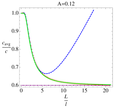
Figure 1: Ratio of velocities $c_{avg}/c$ plotted over the ratio of period length $L$ and frontwidth $l$ for a sinusoidal variation of excitation threshold $u_{2}\left(x\right)=0.35+A\sin\left(2\pi x/L\right).$ Projection method (green solid line) shows excellent agreement with numerical results (red crosses), 2nd order averaging (blue dashed line) fails for large period lengths. The harmonic mean velocity (purple dash-dotted line) gives the approximate average velocity for large period lengths.

IV.4 2nd order averaging for a sinusoidally varied fixed point parameter $u_{3}$

The heterogeneous reaction function (36) is

$$R\left(u,x\right) =-u\left(u-u_{2}\right)\left(u-\left(1+A\sin\left(2\pi x/L\right)\right)\right)$$

$$=\left(1+A\sin\left(2\pi x/L\right)\right)u\left(u-u_{2}\right)-u^{2}\left(u-u_{2}\right)$$

$$=\left(1+g^{\prime}\left(\dfrac{x}{L}\right)\right)f\left(u\right)-a\left(u\right).$$ (64)

The integration constant for $G$ is determined so that $\left\langle G\right\rangle=\frac{A^{2}\left(u_{2}-2\right)}{8\pi^{2}\left(3u_{2}-5\right)},$ (45). The ODE for the position of the front has the same form as for a variation of $u_{2},$

$$\Theta_{2}^{A}\left(\phi\right)=H_{1}\sin\left(\frac{2\pi\phi}{L}\right)+H_{2}\cos\left(\frac{2\pi\phi}{L}\right)\\ +H_{3}\sin\left(\frac{4\pi\phi}{L}\right)+H_{4}\cos\left(\frac{4\pi\phi}{L}\right)+H_{5},$$ (65)

The constants $H_{1}$ up to $H_{5}$ are listed in the appendix, see (84). The average velocity (48) is computed numerically.

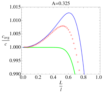
Figure 2: Velocity overshoot for a sinusoidal variation of excitation threshold $u_{2}\left(x\right)=0.35+A\sin\left(2\pi x/L\right),$ predicted by 2nd order averaging (blue dashed line) in qualitative agreement with numerical results (red crosses). Projection method (green solid line) fails for small period lengths.

Figure 3: Velocity overshoot for a sinusoidal variation of $u_{3}\left(x\right)=1+A\sin\left(2\pi x/L\right)$ and $u_{2}=0.35$ predicted by 2nd order averaging (blue dashed line) in agreement with numerical results (red crosses). Propagation failure is predicted qualitatively by projection method (green solid line), which fails for small period lengths.

V Comparison of Analytical and Numerical Results

The PDE for the heterogeneous Schlögl model is solved numerically with a simple finite differences Euler forward scheme and the average velocity is obtained by a linear fit of the space over time data over an integer multiple of period lengths. Data near to the boundaries have to be neglected because of boundary effects.

V.1 Variation of excitation threshold $u_{2}$

A sinusoidally varied excitation threshold $u_{2}\left(x\right)=u_{2}+A\sin\left(\frac{2\pi x}{L}\right)$ leads to an average velocity

$$c_{avg,\,u_{2}}=\left(c^{2}-\frac{4A^{2}\left(\left(u_{2}-1\right)^{2}L^{2}+2\pi^{2}\right)}{\left(2u_{2}^{3}-3u_{2}^{2}+u_{2}\right)^{2}L^{6}}\right.\\ \left.\vphantom{c^{2}-\frac{4A^{2}\left(\left(u_{2}-1\right)^{2}L^{2}+2\pi^{2}\right)}{\left(2u_{2}^{3}-3u_{2}^{2}+u_{2}\right)^{2}L^{6}}}\times\frac{\left(u_{2}^{2}L^{2}+2\pi^{2}\right)\left(L^{2}\left(1-2u_{2}\right)^{2}+8\pi^{2}\right)\sin^{2}\left(2u_{2}\pi\right)}{\left(\cosh\left(\frac{4\sqrt{2}\pi^{2}}{L}\right)-\cos\left(4u_{2}\pi\right)\right)}\right)^{\frac{1}{2}}$$ (66)

obtained by the projection method according to the formula (55). For intermediate and large period lengths, the agreement between (66) and numerical results is excellent, see Fig. 1. The averaging method in 2nd order gives good results for small period lengths but fails for large period lengths, as could be expected because the period length is used as the small parameter for the perturbation expansion (although 1st order averaging does not fail for large period lengths).

V.2 Velocity overshoot

For period lengths smaller than the front width, the numerical results for the sinusoidally varied excitation threshold show a small velocity overshoot. The results obtained in 2nd order averaging predict this overshoot qualitatively at the right size of period lengths. Eq. (66) shows a plateau-like behavior indicating the transcendental smallness of the results obtained with the projection method for small period lengths, see Fig. 2.

For a sinusoidal variation of the fixed point parameter $u_{3}\left(x\right)=1+A\sin\left(\frac{2\pi x}{L}\right),$ a large velocity overshoot is found numerically, again predicted qualitatively by 2nd order averaging and missed by the projection method, which gives an analytical solution for the average velocity

$$c_{avg,\,u_{3}}=\left(c^{2}-\frac{A^{2}\left(\left(u_{2}-1\right)^{2}L^{2}+8\pi^{2}\right)}{\left(2u_{2}^{3}-3u_{2}^{2}+u_{2}\right)^{2}L^{6}}\right.\\ \left.\vphantom{c^{2}-\frac{A^{2}\left(u_{2}^{2}L^{2}+2\pi^{2}\right)\left(\left(u_{2}-1\right)^{2}L^{2}+8\pi^{2}\right)}{\left(2u_{2}^{3}-3u_{2}^{2}+u_{2}\right)^{2}L^{6}\left(\cosh\left(\frac{4\sqrt{2}\pi^{2}}{L}\right)-\cos\left(4u_{2}\pi\right)\right)}}\times\frac{\left(L^{2}\left(1-2u_{2}\right)^{2}+8\pi^{2}\right)\left(u_{2}^{2}L^{2}+2\pi^{2}\right)\sin^{2}\left(2u_{2}\pi\right)}{\left(\cosh\left(\frac{4\sqrt{2}\pi^{2}}{L}\right)-\cos\left(4u_{2}\pi\right)\right)}\right)^{\frac{1}{2}}.$$ (67)

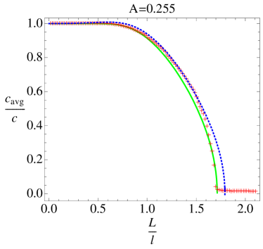
Figure 4: Propagation failure for a sinusoidal variation of excitation threshold $u_{2}\left(x\right)=0.35+A\sin\left(2\pi x/L\right)$ occurs if the average velocity obtained by numerical simulation (red crosses) drops to zero and can be predicted by projection method (green solid line) and qualitatively by 2nd order averaging (blue dashed line).

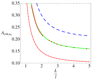
Figure 5: The critical amplitude for which propagation failure occurs for a sinusoidal variation of the excitation threshold $u_{2}\left(x\right)=u_{2}+A\sin\left(2\pi x/L\right),$ obtained by the projection method, is a monotonically decreasing function for all values of $u_{2}$ and shown for $u_{2}=0.3$ (blue dashed line) and $u_{2}=0.4$ (red dash-dotted line). The results for a value of $u_{2}=0.35$ (green solid line) are compared to numerical simulations (red dots).

V.3 Propagation failure

With the condition for propagation failure, $c_{avg}=0,$ the results for the average velocity obtained with the projection method allows to determine the critical amplitude for which propagation failure occurs. For the case of a sinusoidally varied excitation threshold, this gives

$$A_{crit,\,u_{2}}\left(L\right)=\frac{L^{3}\sqrt{\cosh\left(\frac{4\sqrt{2}\pi^{2}}{L}\right)-\cos\left(4\pi u_{2}\right)}}{2\sqrt{2}\sqrt{L^{2}\left(u_{2}-1\right)^{2}+2\pi^{2}}}\\ \times\frac{\csc\left(2\pi u_{2}\right)\left(1-2u_{2}\right)^{2}\left(1-u_{2}\right)u_{2}}{\sqrt{L^{2}u_{2}^{2}+2\pi^{2}}\sqrt{L^{2}\left(1-2u_{2}\right)^{2}+8\pi^{2}}},$$ (68)

which is a monotonically decreasing function for all values of the system parameter $u_{2}.$ This means that for a fixed amplitude large enough, propagation failure occurs for all period lengths larger than a certain critical period length, see Fig. 4. For the choice of parameters shown in Fig. 4, the result of 2nd order averaging can predict the propagation failure, but if propagation failure occurs at larger period lengths, it fails badly to do so. Comparison of (68) with numerical results shows very good agreement, see Fig. 5.

For a sinusoidal variation of the reaction coefficient $k\left(x\right)=1+A\sin\left(\frac{2\pi x}{L}\right)$ a different behavior occurs. The average velocity obtained with the projection method is given as

$$c_{avg,\,k}=\left(c^{2}-\frac{A^{2}\left(\left(u_{2}-1\right)^{2}L^{2}+2\pi^{2}\right)}{4u_{2}^{2}\left(u_{2}\left(2u_{2}-3\right)+1\right)^{2}}\right.\\ \left.\vphantom{c^{2}-\frac{A^{2}\left(\left(u_{2}-1\right)^{2}L^{2}+2\pi^{2}\right)}{4u_{2}^{2}\left(u_{2}\left(2u_{2}-3\right)+1\right)^{2}}}\times\frac{\left(u_{2}^{2}L^{2}+2\pi^{2}\right)\left(L^{2}\left(1-2u_{2}\right)^{2}+8\pi^{2}\right)^{2}\sin^{2}\left(2u_{2}\pi\right)}{L^{8}\left(\cosh\left(\frac{4\sqrt{2}\pi^{2}}{L}\right)-\cos\left(4u_{2}\pi\right)\right)}\right)^{\frac{1}{2}}$$ (69)

and shows, for a certain range of the system parameter $u_{2}$ and in qualitative agreement with numerical simulations, a minimum for a finite period length, see Fig. 6. For a value of the amplitude large enough and slightly different values of the system parameter $u_{2},$ the projection method predicts propagation failure occurring for an interval of period lengths, see Fig. 7, and propagation is possible for larger and smaller period lengths. Comparison with numerical results shows qualitative agreement, see Fig. 8. The critical amplitude for which propagation failure occurs is given as

$$A_{crit,\,k}\left(L\right)=\frac{\sqrt{2}L^{4}\sqrt{\cosh\left(\frac{4\sqrt{2}\pi^{2}}{L}\right)-\cos\left(4\pi u_{2}\right)}}{\sqrt{L^{2}\left(u_{2}-1\right)^{2}+2\pi^{2}}}\\ \times\frac{\csc\left(2\pi u_{2}\right)\left(1-2u_{2}\right)^{2}\left(1-u_{2}\right)u_{2}}{\sqrt{L^{2}u_{2}^{2}+2\pi^{2}}\left(L^{2}\left(1-2u_{2}\right)^{2}+8\pi^{2}\right)}.$$ (70)

and is shown for different values of $u_{2}$ in Fig. 9. There one can see again the fact that propagation fails for an interval of period lengths: the critical amplitude has a minimum for a finite period length and is not a monotonically decreasing function.

For most cases of a variation of $u_{3},$ the critical amplitude for which propagation failure occurs is a monotonically decreasing function, but for a very small range of the system parameter $u_{2},$ propagation failure can occur for an interval of period lengths (not shown).

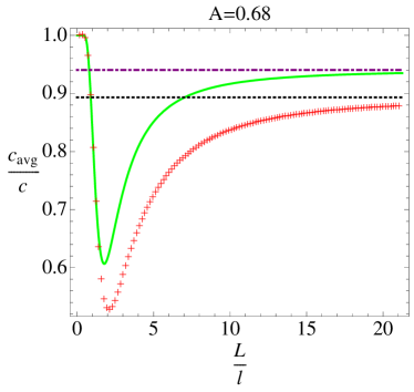
Figure 6: Ratio of velocities $c_{avg}/c$ plotted over the ratio of period length $L$ and front width $l$ for a sinusoidal variation of $k\left(x\right)=1+A\sin\left(2\pi x/L\right)$ and $u_{2}=0.38.$ The average velocity shows a minimum and the numerical solution (red crosses) approaches the harmonic mean velocity (black dashed line) from below. The solution obtained by projection method (green solid line) approaches a different limit (purple dot-dashed line).

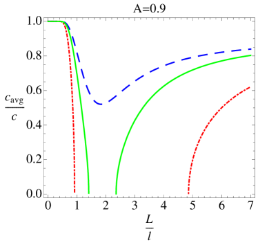
Figure 7: The ratio of velocities $c_{avg}/c$ either shows an interval of period lengths for which propagation failure occurs or a minimum for a sinusoidal variation of $k\left(x\right)=1+A\sin\left(2\pi x/L\right),$ depending on the value of $u_{2}=0.35$ (blue dashed line), $u_{2}=0.425$ (red dot-dashed line), $u_{2}=0.38$ (green solid line).

V.4 Front velocity in the limit of large period lengths

The average velocity obtained with the projection method allows to determine the limit for large period lengths. For the case of the sinusoidal variation of excitation threshold $u_{2},$ this limit is given as

$$\lim_{L\rightarrow\infty}c_{avg,\,u_{2}} =\sqrt{c^{2}-2A^{2}},$$ (71)

which agrees with the harmonic mean of the velocities computed according to (14). The numerical solution approaches the limit (71) from above, as shown in Fig. 1. The limit of the average velocity

$$\lim_{L\rightarrow\infty}c_{avg,\,u_{3}} =\sqrt{c^{2}-\frac{1}{2}A^{2}},$$ (72)

for the sinusoidal variation of $u_{3}$ also agrees with the harmonic mean of the velocities and with numerical results (not shown).

For the sinusoidal variation of reaction coefficient $k$ the limit for large period lengths of (69) is

$$\lim_{L\rightarrow\infty}c_{avg,\,k} =c\sqrt{1-\frac{A^{2}}{4}},$$ (73)

which does not agree with the harmonic mean of the velocities,

$$\bar{c}_{harm,\,k} =\pi c\frac{1}{\left(\frac{K\left(\frac{2A}{A-1}\right)}{\sqrt{1-A}}+\frac{K\left(\frac{2A}{A+1}\right)}{\sqrt{1+A}}\right)},$$ (74)

where $K\left(x\right)$ is the complete elliptic integral of the first kind. The numerical solution approaches the harmonic mean of the velocities (74) from below, see Fig. 6, Fig. 8. The velocity of the unperturbed general Schlögl model has the same square root dependence on the reaction coefficient $k$ as on the diffusion coefficient $D,$ see (4). It follows that the limit of large period lengths of the average velocity for the case of a sinusoidal variation of the diffusion coefficient $D\left(x\right)=1+A\sin\left(2\pi x/L\right)$ is the same as (74), which was checked by numerical simulations (not shown).

VI Discussion

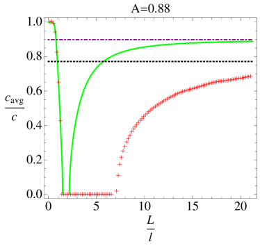
Figure 8: Interval of period lengths for which propagation failure occurs for a sinusoidal variation of reaction coefficient $k\left(x\right)=1+A\sin\left(2\pi x/L\right),$ predicted by projection method (green solid line) in qualitative agreement with numerical results (red crosses). The limit for large period lengths of the numerical results is given by the harmonic mean of the velocities (black dashed line), the analytical solution approaches a different limit (purple dot-dashed line).

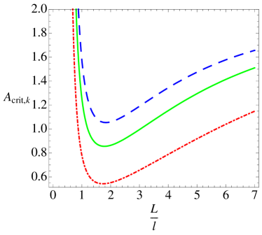
Figure 9: The critical amplitude for which propagation failure occurs obtained by projection method for a sinusoidal variation of $k\left(x\right)=1+A\sin\left(2\pi x/L\right)$ shows a minimum for all values of $u_{2}=0.35$ (blue dashed line), $u_{2}=0.425$ (red dot-dashed line) and $u_{2}=0.38$ (green solid line).

Infinitely extended spatially varied reaction parameters of the Schlögl model are considered and the effects on the propagation velocity are studied. The applied perturbation methods seem to work best for a variation of excitation threshold $u_{2},$ the reason is probably that the front profile (3) does not depend on this parameter. The projection method works worse for a variation of the reaction coefficient $k$ than for all other variations, even not predicting the correct limit of the average velocity for large period lengths. This could be connected to the fact that the velocity of the homogeneous case (4) shows a linear dependence on the fixed point parameters but a square root dependence on $k.$ The ODE for the position of the front obtained in 1st order averaging is equivalent to the one obtained with the projection method, and both fail generally for small period lengths due to the transcendentally small dependence of $\Theta_{1}\left(\phi\right)$ on the period length. This causes the plateau in the plots of the average velocity for small period lengths in all solutions obtained with the projection method. The solutions obtained in 2nd order averaging agree qualitatively with the numerical simulations and can predict the size and the value of the period lengths for which velocity overshoots occur, but generally fail for large period lengths. A small velocity overshoot up to $1.5\%$ is found for a variation of the excitation threshold $u_{2}$ with period lengths slightly smaller than the front width. A similar velocity overshoot was found for period lengths for a variation of the excitation threshold in the modified Oregonator model Schebesch and Engel (1998). For a variation of $u_{3},$ a larger velocity overshoot up to $25\%$ is found, which occurs at period lengths of approximately the same size as the velocity overshoot in the case of the variation of $u_{2}.$ Propagation failure occurs in both cases for amplitudes large enough and all period lengths larger than a certain critical period length. For a variation of the reaction coefficient $k,$ and for a small range of values of the system parameter $u_{2}$ in the case of a variation of $u_{3},$ we find an interval of period lengths for which propagation failure occurs. All computations were done for a sinusoidal as well as for a rectangular variation of the parameters, which show qualitatively the same effects. The amplitude $A$ and the period length $L$ are more important in affecting the front velocity than the shape of the heterogeneities.

Appendix A

The ODE for the position of the front for a sinusoidal variation of $u_{1},\,u_{2},\,u_{3}$ and $k$ obtained with the projection method is

$$\frac{\textrm{d}}{\textrm{d}t}\phi\left(t\right) =c-\frac{\epsilon A}{K_{c}}\intop_{-\infty}^{\infty}e^{c\xi}U_{c}^{\prime}\left(\xi\right)\sin\left(2\pi\left(\xi+\phi\left(t\right)\right)/L\right)$$

$$\times\left(U_{c}\left(\xi\right)-Z_{1}\right)\left(U_{c}\left(\xi\right)-Z_{2}\right)\left(Z_{4}u+Z_{3}\right)\textrm{d}\xi$$

$$=c+\epsilon C_{1}\left(C_{2}\sin\left(\frac{2\pi\phi(t)}{L}\right)+C_{3}\cos\left(\frac{2\pi\phi(t)}{L}\right)\right),$$ (75)

with

$$C_{1} =-\frac{A\sin\left(\sqrt{2}c\pi\right)}{\left(2c^{3}-c\right)L^{4}\left(\cos\left(2\sqrt{2}c\pi\right)-\cosh\left(\frac{4\sqrt{2}\pi^{2}}{L}\right)\right)},$$

$$C_{2} =\cosh\left(\frac{2\sqrt{2}\pi^{2}}{L}\right)\sin\left(\sqrt{2}c\pi\right)H_{1}$$

$$+2\cos\left(\sqrt{2}c\pi\right)\sinh\left(\frac{2\sqrt{2}\pi^{2}}{L}\right)H_{2},$$

$$C_{3} =2\cosh\left(\frac{2\sqrt{2}\pi^{2}}{L}\right)\sin\left(\sqrt{2}c\pi\right)H_{2}$$

$$-\cos\left(\sqrt{2}c\pi\right)\sinh\left(\frac{2\sqrt{2}\pi^{2}}{L}\right)H_{1},$$ (76)

$$H_{1}=32\pi^{4}Z_{4}+L^{4}\left(2\sqrt{2}\left(\left(2Z_{1}+2Z_{2}-3\right)Z_{4}-2Z_{3}\right)c^{3}\right.\\ \left.\vphantom{2Z_{4}c^{4}+2\sqrt{2}\left(\left(2Z_{1}+2Z_{2}-3\right)Z_{4}-2Z_{3}\right)c^{3}}-c^{2}\left(-12Z_{1}\left(Z_{2}-1\right)+12Z_{2}-11\right)Z_{4}\right.\\ \left.\vphantom{2Z_{4}c^{4}+2\sqrt{2}\left(\left(2Z_{1}+2Z_{2}-3\right)Z_{4}-2Z_{3}\right)c^{3}}+2Z_{4}c^{4}-12c^{2}\left(Z_{1}+Z_{2}-1\right)Z_{3}\right.\\ \left.\vphantom{2Z_{4}c^{4}+2\sqrt{2}\left(\left(2Z_{1}+2Z_{2}-3\right)Z_{4}-2Z_{3}\right)c^{3}}+\sqrt{2}c\left(Z_{1}\left(4-6Z_{2}\right)+4Z_{2}-3\right)Z_{4}\right.\\ \left.\vphantom{2Z_{4}c^{4}+2\sqrt{2}\left(\left(2Z_{1}+2Z_{2}-3\right)Z_{4}-2Z_{3}\right)c^{3}}+\sqrt{2}2c\left(Z_{1}\left(3-6Z_{2}\right)+3Z_{2}-2\right)Z_{3}\right)\\ +L^{2}\left(24\sqrt{2}\pi^{2}\left(2Z_{3}+\left(-2Z_{1}-2Z_{2}+3\right)Z_{4}\right)c\right.\\ \left.\vphantom{24\sqrt{2}\pi^{2}\left(2Z_{3}+\left(-2Z_{1}-2Z_{2}+3\right)Z_{4}\right)c}+4\pi^{2}\left(-12Z_{1}\left(Z_{2}-1\right)+12Z_{2}-11\right)Z_{4}\right.\\ \left.\vphantom{24\sqrt{2}\pi^{2}\left(2Z_{3}+\left(-2Z_{1}-2Z_{2}+3\right)Z_{4}\right)c}+\pi^{2}48\left(Z_{1}+Z_{2}-1\right)Z_{3}-48\pi^{2}Z_{4}c^{2}\right),$$ (77)

$$H_{2}=L8\pi^{3}\left(2\sqrt{2}Z_{3}-\left(4c+\sqrt{2}\left(2Z_{1}+2Z_{2}-3\right)\right)Z_{4}\right)\\ +L^{3}\pi\left(\left(6\sqrt{2}\left(2Z_{1}+2Z_{2}-3\right)c^{2}+\left(24Z_{1}\left(Z_{2}-1\right)-24Z_{2}\right)c\right.\right.\\ \left.\left.+22c+8c^{3}+\sqrt{2}\left(Z_{1}\left(4-6Z_{2}\right)+4Z_{2}-3\right)\right)Z_{4}\right.\\ \left.-2\left(6\sqrt{2}c^{2}+12\left(Z_{1}+Z_{2}-1\right)c\right.\right.\\ \left.\left.+\sqrt{2}\left(-3Z_{2}+Z_{1}\left(6Z_{2}-3\right)+2\right)\right)Z_{3}\right).$$ (78)

Appendix B

With the help of the averaging method in 2nd order an ODE for the position of the front for a sinusoidal variation of the excitation threshold is derived

$$\Theta_{2}^{A}\left(\phi\right)=H_{1}\sin\left(\frac{2\pi\phi}{L}\right)+H_{2}\cos\left(\frac{2\pi\phi}{L}\right)\\ +H_{3}\sin\left(\frac{4\pi\phi}{L}\right)+H_{4}\cos\left(\frac{4\pi\phi}{L}\right)+H_{5},$$ (79)

$$H_{1} =\frac{A}{\sqrt{2}D_{1}}\left(\sin\left(2\sqrt{2}c\pi\right)\sinh\left(\frac{2\sqrt{2}\pi^{2}}{L}\right)J_{1}\right.$$

$$\left.\vphantom{\sin\left(2\sqrt{2}c\pi\right)\sinh\left(\frac{2\sqrt{2}\pi^{2}}{L}\right)J_{1}}-4\cosh\left(\frac{2\sqrt{2}\pi^{2}}{L}\right)\sin^{2}\left(\sqrt{2}c\pi\right)J_{3}\right)$$

$$H_{2} =\frac{\sqrt{2}A}{D_{1}}\left(\cosh\left(\frac{2\sqrt{2}\pi^{2}}{L}\right)J_{1}\sin^{2}\left(\sqrt{2}c\pi\right)\right.$$

$$\left.\vphantom{\cosh\left(\frac{2\sqrt{2}\pi^{2}}{L}\right)J_{1}\sin^{2}\left(\sqrt{2}c\pi\right)}+\sin\left(2\sqrt{2}c\pi\right)\sinh\left(\frac{2\sqrt{2}\pi^{2}}{L}\right)J_{3}\right)$$

$$H_{3} =-\frac{A^{2}}{2D_{2}}\left(4\cosh\left(\frac{4\sqrt{2}\pi^{2}}{L}\right)J_{4}\sin^{2}\left(\sqrt{2}c\pi\right)\right.$$

$$\left.\vphantom{4\cosh\left(\frac{4\sqrt{2}\pi^{2}}{L}\right)J_{4}\sin^{2}\left(\sqrt{2}c\pi\right)}+\sin\left(2\sqrt{2}c\pi\right)\sinh\left(\frac{4\sqrt{2}\pi^{2}}{L}\right)J_{2}\right)$$

$$H_{4} =-\frac{A^{2}}{D_{2}}\left(\cosh\left(\frac{4\sqrt{2}\pi^{2}}{L}\right)\sin^{2}\left(\sqrt{2}c\pi\right)J_{2}\right.$$

$$\left.\vphantom{\cosh\left(\frac{4\sqrt{2}\pi^{2}}{L}\right)\sin^{2}\left(\sqrt{2}c\pi\right)J_{2}}-\sin\left(2\sqrt{2}c\pi\right)\sinh\left(\frac{4\sqrt{2}\pi^{2}}{L}\right)J_{4}\right)$$

$$H_{5} =\frac{A^{2}c}{8\pi^{2}}$$ (80)

$$J_{1} =c^{2}\left(1-2c^{2}\right)L^{4}+4\left(12c^{2}-1\right)\pi^{2}L^{2}-32\pi^{4},$$

$$J_{2} =c^{2}\left(2c^{2}-1\right)L^{4}+16\left(1-12c^{2}\right)\pi^{2}L^{2}+512\pi^{4},$$

$$J_{3} =2c\pi L\left(\left(1-4c^{2}\right)L^{2}+16\pi^{2}\right),$$

$$J_{4} =4c\pi L\left(\left(1-4c^{2}\right)L^{2}+64\pi^{2}\right),$$ (81)

$$D_{1} =\left(2c^{3}-c\right)\pi L^{5}\left(\cos\left(2\sqrt{2}c\pi\right)-\cosh\left(\frac{4\sqrt{2}\pi^{2}}{L}\right)\right),$$

$$D_{2} =4\left(2c^{3}-c\right)\pi^{2}L^{4}\left(\cos\left(2\sqrt{2}c\pi\right)-\cosh\left(\frac{8\sqrt{2}\pi^{2}}{L}\right)\right).$$ (82)

Appendix C

For the sinusoidal variation of the fixed point parameter $u_{3},$ 2nd order averaging gives an ODE for the position of the front

$$\Theta_{2}^{A}\left(\phi\right)=H_{1}\sin\left(\frac{2\pi\phi}{L}\right)+H_{2}\cos\left(\frac{2\pi\phi}{L}\right)\\ +H_{3}\sin\left(\frac{4\pi\phi}{L}\right)+H_{4}\cos\left(\frac{4\pi\phi}{L}\right)+H_{5},$$ (83)

with

$$H_{1} =-\frac{A}{D_{1}}\sin\left(\sqrt{2}c\pi\right)\left(\cos\left(\sqrt{2}c\pi\right)\sinh\left(\frac{2\sqrt{2}\pi^{2}}{L}\right)J_{1}\right.$$

$$\left.\vphantom{\cos\left(\sqrt{2}c\pi\right)\sinh\left(\frac{2\sqrt{2}\pi^{2}}{L}\right)J_{1}}+\cosh\left(\frac{2\sqrt{2}\pi^{2}}{L}\right)\sin\left(\sqrt{2}c\pi\right)J_{2}\right),$$

$$H_{2} =-\frac{A}{D_{1}}\sin\left(\sqrt{2}c\pi\right)\left(\cosh\left(\frac{2\sqrt{2}\pi^{2}}{L}\right)\sin\left(\sqrt{2}c\pi\right)J_{1}\right.$$

$$\left.\vphantom{\cosh\left(\frac{2\sqrt{2}\pi^{2}}{L}\right)\sin\left(\sqrt{2}c\pi\right)J_{1}}-\cos\left(\sqrt{2}c\pi\right)\sinh\left(\frac{2\sqrt{2}\pi^{2}}{L}\right)J_{2}\right),$$

$$H_{3} =-\frac{A^{2}}{D_{2}}\sin\left(\sqrt{2}c\pi\right)\left(\cosh\left(\frac{4\sqrt{2}\pi^{2}}{L}\right)\sin\left(\sqrt{2}c\pi\right)J_{4}\right.$$

$$\left.\vphantom{\cosh\left(\frac{4\sqrt{2}\pi^{2}}{L}\right)\sin\left(\sqrt{2}c\pi\right)J_{4}}-\cos\left(\sqrt{2}c\pi\right)\sinh\left(\frac{4\sqrt{2}\pi^{2}}{L}\right)J_{3}\right),$$

$$H_{4} =\frac{A^{2}}{D_{2}}\sin\left(\sqrt{2}c\pi\right)\left(\cosh\left(\frac{4\sqrt{2}\pi^{2}}{L}\right)\sin\left(\sqrt{2}c\pi\right)J_{3}\right.$$

$$\left.\vphantom{\cosh\left(\frac{4\sqrt{2}\pi^{2}}{L}\right)\sin\left(\sqrt{2}c\pi\right)J_{3}}+\cos\left(\sqrt{2}c\pi\right)\sinh\left(\frac{4\sqrt{2}\pi^{2}}{L}\right)J_{4}\right),$$

$$H_{5} =\frac{A^{2}c}{8\pi^{2}},$$ (84)

$$J_{1} =c^{2}\left(\sqrt{2}\left(2-3u_{2}\right)+2c\left(\sqrt{2}c+3u_{2}-3\right)\right)L^{4}+32\sqrt{2}\pi^{4}$$

$$-4\pi^{2}\left(\sqrt{2}\left(2-3u_{2}\right)+6c\left(2\sqrt{2}c+3u_{2}-3\right)\right)L^{2},$$

$$J_{2} =4\pi L\left(c\left(c\left(-4\sqrt{2}c-9u_{2}+9\right)+\sqrt{2}\left(3u_{2}-2\right)\right)L^{2}\right.$$

$$\left.\vphantom{c\left(c\left(-4\sqrt{2}c-9u_{2}+9\right)+\sqrt{2}\left(3u_{2}-2\right)\right)L^{2}}+4\pi^{2}\left(4\sqrt{2}c+3u_{2}-3\right)\right),$$

$$J_{3} =c\left(-2c^{3}-6\sqrt{2}\left(u_{2}-1\right)c^{2}+\left(-6\left(u_{2}-3\right)u_{2}-11\right)c\right)L^{4}$$

$$+16\pi^{2}\left(12c^{2}+18\sqrt{2}\left(u_{2}-1\right)c+6\left(u_{2}-3\right)u_{2}+11\right)L^{2}$$

$$-512\pi^{4}+3\sqrt{2}cL^{4}\left(u_{2}-1\right)^{2},$$

$$J_{4} =4\pi L\left(\left(-18\sqrt{2}\left(u_{2}-1\right)c^{2}-2\left(6\left(u_{2}-3\right)u_{2}+11\right)c\right)L^{2}\right)$$

$$+12\sqrt{2}\pi L^{3}\left(u_{2}-1\right)^{2}-32\pi L^{3}c^{3}$$

$$+128\pi^{3}L\left(4c+3\sqrt{2}\left(u_{2}-1\right)\right),$$ (85)

and $D_{1},\,D_{2}$ are given as in (82).

References

• Kapral and Showalter (1995) R. Kapral and K. Showalter, Chemical waves and patterns (Kluwer Academic Pub, 1995).
• Keener and Sneyd (2008) J. Keener and J. Sneyd, Mathematical Physiology: Cellular Physiology (Springer, 2008).
• Cross and Hohenberg (1993) M. Cross and P. Hohenberg, Reviews of Modern Physics 65, 851 (1993).
• Bode et al. (2002) M. Bode, A. Liehr, C. Schenk, and H. Purwins, Physica D: Nonlinear Phenomena 161, 45 (2002).
• Keener (2000a) J. Keener, SIAM Journal on Applied Mathematics 61, 317 (2000a).
• Teramoto et al. (2009) T. Teramoto, X. Yuan, M. Bär, and Y. Nishiura, Physical Review E 79, 46205 (2009).
• Schütz et al. (1995) P. Schütz, M. Bode, and H. Purwins, Physica D: Nonlinear Phenomena 82, 382 (1995).
• Bode (1997) M. Bode, Physica D: Nonlinear Phenomena 106, 270 (1997).
• Xin (2000) J. Xin, SIAM REVIEW 42, 161 (2000).
• Nishiura et al. (2007) Y. Nishiura, T. Teramoto, X. Yuan, and K. Ueda, Chaos: An Interdisciplinary Journal of Nonlinear Science 17, 037104 (2007).
• Bär et al. (2002) M. Bär, E. Meron, and C. Utzny, Chaos: An Interdisciplinary Journal of Nonlinear Science 12, 204 (2002).
• Bub et al. (2002) G. Bub, A. Shrier, and L. Glass, Physical review letters 88, 58101 (2002).
• Krug et al. (1990) H. Krug, L. Pohlmann, and L. Kuhnert, Journal of Physical Chemistry 94, 4862 (1990).
• Schebesch and Engel (1998) I. Schebesch and H. Engel, Physical Review E 57, 3905 (1998).
• Engel (1985) A. Engel, Physics letters. A 113, 139 (1985).
• Mikhailov et al. (1983) A. Mikhailov, L. Schimansky-Geier, and W. Ebeling, Phys. Lett. A 46, 453 (1983).
• Schimansky-Geier et al. (1983) L. Schimansky-Geier, A. Mikhailov, and W. Ebeling, Annalen der Physik(Leipzig) 40, 277 (1983).
• Zeldovich and Frank-Kamenetsky (1938) Y. Zeldovich and D. Frank-Kamenetsky, in Dokl. Akad. Nauk SSSR (1938), vol. 19, pp. 693–697.
• Schlögl (1972) F. Schlögl, Zeitschrift für Physik A Hadrons and Nuclei 253, 147 (1972).
• Mikhailov (1990) A. Mikhailov, Foundations of Synergetics (Springer, 1990).
• Kulka et al. (1995) A. Kulka, M. Bode, and H. Purwins, Physics Letters A 203, 33 (1995).
• Keener (2000b) J. Keener, Principles of Applied Mathematics: Transformation and Approximation (Perseus Books Group, 2000b).
• Bogoliubov and Mitropolsky (1961) N. Bogoliubov and Y. Mitropolsky, Asymptotic methods in the theory of non-linear oscillations (Hindustan Publ. Corp. Delhi, 1961).
• Keener (2000c) J. Keener, Physica D: Nonlinear Phenomena 136, 1 (2000c).