Adiabatic Heating of Contracting Turbulent Fluids

Abstract

Turbulence influences the behavior of many astrophysical systems, frequently by providing non-thermal pressure support through random bulk motions. Although turbulence is commonly studied in systems with constant volume and mean density, turbulent astrophysical gases often expand or contract under the influence of pressure or gravity. Here, we examine the behavior of turbulence in contracting volumes using idealized models of compressed gases. Employing numerical simulations and an analytical model, we identify a simple mechanism by which the turbulent motions of contracting gases “adiabatically heat”, experiencing an increase in their random bulk velocities until the largest eddies in the gas circulate over a “Hubble” time of the contraction. Adiabatic heating provides a mechanism for sustaining turbulence in gases where no large-scale driving exists. We describe this mechanism in detail and discuss some potential applications to turbulence in astrophysical settings.

1. Introduction

Turbulence – the bulk random motion of a gas or fluid – is ubiquitous in astrophysics. Turbulence can be generated by instabilities, including gravitational (Jeans, 1902), shear (von Helmholtz, 1868; Kelvin, 1871), convective (Rayleigh, 1884; Taylor, 1950), and magnetorotational (Balbus & Hawley, 1991). For overviews, see Elmegreen & Scalo (2004) and McKee & Ostriker (2007). Given its wide-spread importance, turbulence remains a critical area for astrophysical research.

Supersonic turbulence has been studied in great detail with numerical simulations. For instance, supersonic isothermal turbulence exhibits a lognormal density distribution, with a width that increases with the Mach number (e.g., Vazquez-Semadeni, 1994; Padoan et al., 1997; Kritsuk et al., 2007; Lemaster & Stone, 2008; Federrath et al., 2010; Price et al., 2011). The properties of supersonic isothermal turbulence appear to be independent of the simulation methodology (e.g., Kitsionas et al., 2009; Price & Federrath, 2010; Bauer & Springel, 2011). Most studies of turbulence have involved gases simulated in a static volume, whereas astrophysical gases often expand or contract under the influence of pressure or gravity. Little is currently known about the detailed structure of expanding or contracting turbulent gases.

In this Letter, we examine the behavior of turbulence during the contraction of a gas arising from pressure or self-gravity. In Section 2, we use simulations to model contracting turbulence and demonstrate that turbulence adiabatically heats during contraction provided the eddy turnover time is shorter than the contraction time. We term this mechanism “adiabatic heating”, and in Section 3 we present an analytical model that successfully describes its behavior. We discuss some potential astrophysical applications of adiabatic heating in Section 4, and summarize and conclude in Section 5.

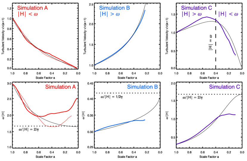
Figure 1.— Contraction of a turbulent gas and the adiabatic heating mechanism. Shown are the RMS turbulent velocities for contracting isothermal simulations with differing Hubble parameters (colored lines). In an initially “slow” contraction (top left panel) where the contraction frequency $|H|$ is lower than the eddy turnover frequency $\omega$, large-scale eddies circulate and the turbulent cascade transfers energy to small scales where it dissipates. Instead, if the contraction frequency is initially higher than the eddy turnover frequency (top center and right panels), the turbulence heats roughly adiabatically at first. As the ratio of eddy turnover and contraction frequencies in the simulations become comparable, whether the turbulence heats or decays as the scale factor $a\to 0$ depends on the evolution of $H(a)$. In a dynamical contraction (top center panel) where $H\propto a^{-3/2}$ the turbulence continues to heat after $\omega$ tracks $|H|$, whereas for constant $H$ (top right panel) it decays. The solid black lines in each panel show the evolution of turbulent velocities predicted by our analytic adiabatic heating model (see Section 3). The dotted lines indicate the model predictions for the synchronized ratio of $\omega/|H|$. To indicate the effect of the forced turbulence initial conditions on the contracting turbulence, the Simulation A panels show two realizations (thick and thin lines).

2. Numerical Simulations of Contracting Turbulence

We use hydrodynamic simulations to study turbulence in a contracting background. We model the contraction by parameterizing the changing physical size $l(t)$ and coordinate scale factor $a=l(t)/L$ of a cubic volume of initial length $L$ through a “Hubble” parameter $H\equiv\dot{a}/a$ that may depend on time $t$. In terms of the proper coordinates within an isotropically contracting volume, the Euler equations connecting derivatives of the density $\rho$, momentum $\rho\vec{v}$, and pressure $p$ are altered by terms that depend on the Hubble parameter as

$$\frac{\partial\rho}{\partial t}=-\nabla\cdot(\rho\vec{v})-3H\rho$$ (1)

$$\frac{\partial\rho\vec{v}}{\partial t}=-\nabla\cdot(\rho\vec{v}\vec{v})-\nabla p-4H\rho\vec{v}$$ (2)

(see, e.g., Section 9 of Peebles, 1980). For an initially constant density and velocity gas without dissipation, these terms give rise to two important scalings well known from cosmology: $\rho\propto a^{-3}$ and $v\propto a^{-1}$. Mass conservation dictates the density scaling, but the presence of dissipation (either through physical viscosity or numerically through the discretized form of Equation 2) implies that the adiabatic velocity scaling does not strictly hold in the contraction of a turbulent gas. How the turbulent velocity evolves depends on how dissipation operates during the contraction, and simulations are required to provide a detailed description.

The simulations were performed using a version of the magnetohydrodynamics code Athena (Stone et al., 2008) modified to model contracting and expanding turbulent gases (see Equations 1 and 2, and below). Athena is a grid code based on the Godunov (1959) method. The calculations use piecewise parabolic reconstruction (Colella & Woodward, 1984) to extrapolate initial states for the Riemann problem between cells and compute final states using an exact solver (Toro, 1999). Cell-averaged conserved quantities are updated using unsplit methods (Gardiner & Stone, 2008). Our modifications to Athena include a Runge-Kutta integrator to evolve a differential equation for the scale factor $a$ that depends on the possibly time-dependent Hubble parameter $H$.

The initial conditions are snapshots of driven isothermal turbulence (with sound speed $c_{s}=1$ and mean density $\bar{\rho}=1$) simulated on an $N=512^{3}$ resolution grid. The random forcing field is generated following Bertschinger (2001), with power input into the two largest modes in the unit ($L=1$) periodic box (e.g., Kritsuk et al., 2007). Driving at intermediate scales produces similar results. A Helmholtz decomposition in Fourier space removes the dilatational component and each forcing field is normalized to maintain an average Mach number $M\approx 6$ when applied as an acceleration ten times per crossing time $t_{\mathrm{cross}}\approx L/2Mc_{s}$. The driving is applied for ten crossing times and then terminated before the contraction initiates. Although we simulate isothermal gases, results relevant for the adiabatic heating mechanism originate from Equations 1 and 2 and should generalize to other adiabatic indices.

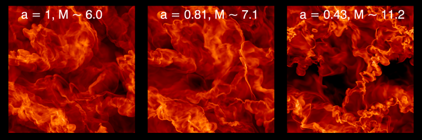
Figure 2.— Adiabatic heating of isothermal supersonic turbulence during contraction. Shown is the logarithmic density distribution through a thin (8/512) slice of Simulation B at three values of the scale factor $a$. Here, the Hubble parameter scales with the inverse dynamical time of the gas. The density maximum in the color map of each panel is scaled by $a^{-3}$, and the dynamic range of each image is $10^{4}$. The turbulence adiabatically heats from the initial Mach number of $M\sim 6$ to $M\sim 11$ as the scale factor decreases by a factor of $\sim 2$. The presence of limited dissipation breaks the perfect adiabatic scaling. The bulk properties of the gas in each panel, including the density distribution and intermittency, behave similarly to static-frame isothermal turbulent gases at the same Mach number.

2.1. Models of Contraction

Two rates characterize the isotropic contraction of a turbulent gas, the contraction frequency $|H|\equiv|\dot{a}/a|$, also called the Hubble parameter ($H<0$ for a contraction), and the eddy turnover frequency

$$\omega\sim\frac{{\rm v}}{aL},$$ (3)

where ${\rm v}$ is the root-mean-squared (RMS) turbulent velocity (for isothermal turbulence ${\rm v}\equiv Mc_{s}$, where $M$ is the typical Mach number and $c_{s}$ is the sound speed). In our simulations, the values of ${\rm v}(t=0)\approx 6c_{s}$, $c_{s}=1$, and $L=1$ imply an initial eddy turnover frequency $\omega(t=0)\approx 6$. To demonstrate the generality of the adiabatic heating mechanism we simulate three different scenarios for the time-dependent relation between $H$ and $\omega$:

Simulation A: an initially “slow exponential contraction”, with $H=$ constant. In this case the scale factor evolves as $a(t)=a_{0}\exp[H(t-t_{0})]$, where $a_{0}=1$ is the initial scale factor and $t_{0}$ is the time when the contraction ensues. We choose a constant Hubble parameter $H=-2$, such that the contraction is slow (i.e., $|H|\ll\omega$) initially. To characterize run-to-run variations, we perform two such simulations differing only in their forced turbulence initial conditions.

Simulation B: an initially “fast dynamical contraction”, with $H\propto\sqrt{\bar{\rho}}$. In this case the contraction time $t_{\mathrm{cont}}\sim|H|^{-1}$ scales with the dynamical time $t_{\mathrm{dyn}}\propto 1/\sqrt{\bar{\rho}}$ set by the mean density $\bar{\rho}\propto a^{-3}$. Starting with an initial value $H(t=t_{0})=H_{0}$, the Hubble parameter varies with the scale factor as $H=H_{0}(a/a_{0})^{-3/2}$. The scale factor decreases with time as $a(t)=a_{0}[3H_{0}(t-t_{0})/2+1]^{2/3}$ (recall that $H_{0}<0$). We set $H_{0}=-20$ to induce an initially fast ($|H|\gg\omega$) contraction.

Simulation C: an initially “fast exponential contraction”, with $H=$ constant. In this case the scale factor evolves with the same time-dependence as in Simulation A, but at a constant contraction frequency ($|H|=20$) such that $|H|\gg\omega$ initially.

2.2. Simulation Results

The properties of contracting turbulence evolve with decreasing scale factor $a$ in a manner that depends upon the ratio of the eddy turnover frequency to the contraction frequency (Figure 1). The simulations demonstrate that if the contraction is slow ($|H|\ll\omega$ initially in Simulation A, left panels), the turbulent velocities decay, whereas if it is fast ($|H|\gg\omega$ initially in Simulations B and C, center and right panels), the turbulent velocities amplify. In a slow contraction, large vortices circulate and nonlinear interactions transfer energy to smaller scales where it is dissipated before the box shrinks appreciably. When the contraction is fast, energy bearing eddies are adiabatically compressed, dissipation primarily operates on small scales, and turbulent velocities increase. In each example in Figure 1, $\omega/|H|$ become comparable (bottom panels). From this trend we surmise that the eddy turnover frequency may eventually “synchronize” with the contraction frequency. Our simulations provide a hint of this behavior, but the synchronized state is not well-explored. Physical considerations suggest the synchronization is stable since the eddies are compressed on their circulation timescale, and the velocities of large eddies should hover around ${\rm v}\sim|H|aL$. If true, as $a\to 0$, the velocities would decrease for constant $|H|$ as observed in Simulations A and C but continue to increase for $|H|\propto a^{-3/2}$ as seen in Simulation B.

Figure 2 shows the projected density distribution through a slice of Simulation B at three scale factors during the contraction. Initially, at $a=1$ (left panel) the gas has a turbulent velocity ${\rm v}\equiv Mc_{s}\approx 6c_{s}$, a lognormal density distribution, and a velocity power spectrum characteristic of supersonic turbulence. Compression during contraction heats the turbulence in the isothermal gas to Mach number $M=7.1$ ($M=11.2$) by scale factor $a=0.81$ ($a=0.43$). As the Mach number increases, the width of the lognormal density distribution increases, the intermittency amplifies, and the velocity power spectrum steepens much in the same way as driven, constant volume isothermal turbulence simulations behave as a function of Mach number (e.g., Price et al., 2011). The increase in turbulent velocities arises from the approximate inverse dependence of velocity on the scale factor during contraction. Since a turbulent cascade transfers large-scale power to small scales where it dissipates, the degree to which the turbulent velocity tracks $a^{-1}$ during the simulation depends on the rate of energy transfer to small scales.

3. Analytical Model of the Adiabatic Heating Mechanism

We model the behavior of turbulent velocities during contraction by calculating the approximate time rate of change of the kinetic energy per unit mass in the gas, including two important terms. A term capturing the effects of adiabatic heating follows from noting that the adiabatic velocity scaling implies ${\rm v}a={\rm v}_{0}$, where ${\rm v}_{0}$ is a constant. Thus

$$\frac{\mathrm{d}}{\mathrm{d}t}\left(\frac{{\rm v}^{2}}{2}\right)_{\mathrm{AH}}={\rm v}\frac{\mathrm{d}{\rm v}}{\mathrm{d}t}=-{\rm v}\frac{{\rm v}_{0}}{a^{2}}\frac{\mathrm{d}a}{\mathrm{d}t}=-H{\rm v}^{2}.$$ (4)

A second term capturing the rate of kinetic energy dissipation is modeled using a parameter $\eta$ that describes the efficiency of the energy cascade. Physically this term would represent viscosity in the Navier-Stokes equation, but in our simulations it arises from dissipative truncation error in the discretization of Euler’s equations. The dissipative term reads

$$\frac{\mathrm{d}}{\mathrm{d}t}\left(\frac{{\rm v}^{2}}{2}\right)_{\mathrm{diss}}=-\eta\frac{{\rm v}^{3}}{aL}.$$ (5)

The relevant length scale in Equation 5 is the driving scale (e.g., Mac Low, 1999), which is the box size $aL$ in our calculations. Simulations of driven incompressible (Gotoh et al., 2002; Beresnyak, 2011) and transonic (Schmidt et al., 2006) turbulence suggest that $\eta\sim 1$. The total rate of change in the turbulent velocity is then

$$\frac{\mathrm{d}{\rm v}}{\mathrm{d}t}=-H{\rm v}-\eta\frac{{\rm v}^{2}}{aL}.$$ (6)

Noting that $aH=\mathrm{d}a/\mathrm{d}t$, and writing the eddy turnover frequency as $\omega({\rm v},a)\sim{\rm v}/aL$, the rate of change of the turbulent velocity with scale factor can be recast as

$$\frac{\mathrm{d}{\rm v}}{\mathrm{d}a}=-\left(1+\eta\frac{\omega}{H}\right)\frac{{\rm v}}{a}.$$ (7)

We will refer to Equation 7 as the “adiabatic heating equation” and it provides quantitative insight into the slow and fast contraction regimes discussed qualitatively above. It shows that the heating of turbulence during contraction is moderated by dissipation with an efficiency proportional to $\sim\omega/|H|$. When the contraction is slow, the dissipative term is larger than the heating term ($\eta\omega/|H|\gg 1$) and the velocity decreases with decreasing scale factor ($\mathrm{d}{\rm v}/\mathrm{d}a>0$). Conversely, when the contraction is fast, the velocity increases with decreasing scale factor ($\mathrm{d}{\rm v}/\mathrm{d}a<0$). Once the eddy turnover and collapse frequencies become comparable and synchronize, whether the velocities grow or decay depends on how $H$ varies with $a$.

Figure 1 depicts the evolution of the turbulent velocity ${\rm v}$ (upper panels) and the ratio of frequencies $\omega/|H|$ (lower panels) obtained from simulations, along with predictions from the adiabatic heating equation using a dissipation parameter fixed at $\eta=1.2$. The model reproduces well the behavior of both properties of turbulence in contracting gases. For simulations where $\omega/|H|\gg 1$ or $\omega/|H|\ll 1$ during the whole computation (left and center panels) the adiabatic heating equation provides an accurate description of the turbulent velocity evolution. In the initially fast contraction with constant $H$ (right panel) the general behavior is also well modeled by the adiabatic heating equation, but the predicted transition from heating to dissipation occurs later in the model than in the numerical computation. These differences may indicate that dissipative effects are delayed in the simulation by an eddy turnover time relative to the analytical model.

The model suggests the adiabatic heating mechanism drives the turbulence in the contraction to an asymptotic relation between $\omega$ and $|H|$ determined by the scale factor dependence of the Hubble parameter. From the adiabatic heating equation and the definition of the eddy turnover frequency, we obtain

$$\frac{d\log(\omega/H)}{d\log(1/a)}=\left(2+\eta\frac{\omega}{H}\right)-\frac{d\log H}{d\log(1/a)}.$$ (8)

The asymptotic relation is approached as $d\log(\omega/H)/d\log(1/a)\to 0$. For $H=~{}$constant we expect $\omega/|H|\to 2/\eta$ (Simulations A and C), while for $H\propto a^{-3/2}$ we have $\omega/|H|\to 1/2\eta$ (Simulation B). We find that the simulations follow the evolution in $\omega/|H|$ predicted by Equation 8 (see Figure 1, lower panels), but can show substantial run-to-run variations (e.g., Simulation A).

The asymptotic relation between the typical turbulent velocities and scale factor can be deduced from Equation 8. By defining

$$\beta\equiv 2+\frac{d\log H}{d\log a},$$ (9)

from the adiabatic heating equation we find simply that ${\rm v}\propto a^{\beta-1}$ once the contraction and eddy turnover frequencies have synchronized.

Although the turbulent velocity roughly tracks the expected scaling ${\rm v}\propto a^{-1}$ before an eddy turnover time elapses, the degree of adiabaticity depends on the small scale dissipation rate. In additional simulations of contracting incompressible isothermal turbulence ($M\sim 0.05$), we have found that even low resolution simulations display almost exact adiabatic heating. For very large isothermal turbulent velocities ($M>10$), we have found that the heating becomes more adiabatic with increasing resolution. This sensible behavior does not affect any of the presented results which have been tested over a wide range of resolutions (from N=64³ to N=512³) and display similar behavior for the same choice of Hubble parameter evolution and initial turbulent velocity.

4. Discussion

Our results have many potential astrophysical applications, but bear especially on the problem of turbulence in giant molecular clouds (GMCs). The properties of GMCs are likely set by turbulence, as the relations between cloud velocity dispersion, size, and mass (Larson, 1981) may reflect properties of turbulence through the velocity structure function (see, e.g., Elmegreen & Scalo, 2004). If so, observations of the dispersion-size relation of GMCs (e.g., Bolatto et al., 2008; Heyer et al., 2009) roughly agree with the properties of compressible turbulence (Ballesteros-Paredes et al., 2006; Kritsuk et al., 2007; Federrath et al., 2010). It has been argued that molecular clouds are in approximate virial equilibrium (Larson, 1981; Solomon et al., 1987) such that turbulent motions either balance the cloud self-gravity or otherwise reflect the depth of the gravitational potential (e.g., Bertoldi & McKee, 1992). This apparent virial balance poses a significant challenge for understanding the origin and evolution of turbulence in molecular clouds, as turbulence should dissipate on a crossing time (e.g., Goldreich & Kwan, 1974) that is shorter than estimates of the cloud lifetime (Blitz & Shu, 1980). The typical GMC lifetime is debated because they may not be in exact balance or gravitationally bound (Hartmann et al., 2001; Dib et al., 2007; Dobbs et al., 2011), and perhaps undergo frequent collisions (e.g., Tasker & Tan, 2009). It remains unclear how turbulence could generically provide support against gravitational collapse since without driving it quickly dissipates (Stone et al., 1998; Mac Low et al., 1998; Cho & Lazarian, 2003).

Our study suggests that the connection between velocity dispersion and size may reflect the competition between adiabatic heating and dissipation. Depending on the nature of the contraction, the adiabatic heating mechanism can enable the typical turbulent velocity to scale with a positive power of the size of a contracting cloud or region, preserving a connection between velocity dispersion and cloud size without an external source for driving the turbulence. From the discussion in Section 3, the observed scalings of ${\rm v}\propto L^{1/2}$ (Solomon et al., 1987; Heyer et al., 2009) require $H\propto a^{-1/2}$. This scaling is quite different than what might occur in a gravitational collapse, where naively one expects $H\propto a^{-3/2}$ and ${\rm v}\propto L^{-1/2}$. If turbulent velocities in GMCs do not originate from gravitational collapse, adiabatic heating may still provide a method for instilling the observed scaling relations through other compression mechanisms.

Although our study has focussed on adiabatic heating in isotropically contracting turbulence, we have examined other scenarios. The inverse process (“adiabatic cooling”) similarly operates in expanding gases. Using simulations with a Hubble parameter $H>0$, we have verified that expanding turbulent gases adiabatically cool if the eddy turnover frequency is less than the expansion frequency $H$. If the expansion is very rapid ($H\gg\omega$) then the turbulence freezes out with ${\rm v}\propto a^{-1}$. Adiabatic cooling may be relevant for turbulent astrophysical systems that rapidly expand, such as those formed in high speed impacts or explosions. We have also simulated anisotropic systems, and found that adiabatic heating and cooling can operate simultaneously in different directions depending on the sign of the effective Hubble parameter for each axis. Applications of anisotropic compressions include studies of shock–turbulence interaction (e.g., Adams & Shariff, 1996).

Some previous works presented ideas related to adiabatic heating. Olson & Sachs (1973) studied analytically the evolution of mean vorticity in incompressible turbulence in expanding universes without dissipation, and commented that in a contracting universe the vorticity would “blow up”. There were early works exploring whether turbulence could seed structure formation (Jones, 1976; Ozernoi, 1978) that considered the adiabatic scaling of velocity with inverse scale factor. The collisional N-body calculations of Scalo & Pumphrey (1982) suggested that turbulence might slow a gravitational collapse. Vazquez-Semadeni et al. (1998) suggested that turbulent velocites might depend on the mean density during collapse. Our description of adiabatic heating has combined and expanded upon some of these concepts.

5. Summary

Using simulations of contracting isothermal turbulent gases performed with the Athena code (Stone et al., 2008), we have identified an “adiabatic heating” mechanism by which random bulk motions are amplified by compression. Adiabatic heating acts to increase the turbulent velocities of a contracting gas if the frequency (or Hubble parameter) $|H|$ of the contraction is larger than the eddy turnover frequency $\omega\sim{\rm v}/aL$ ($L$ is the initial box size, $a$ is the scale factor of the contraction, and ${\rm v}$ is the turbulent velocity). When $|H|\gg\omega$ the cascade of energy from large scales to small scales is limited and dissipation becomes inefficient, thereby allowing the gas velocities to heat with the adiabatic scaling ${\rm v}\propto a^{-1}$ expected from Euler’s equations in a contracting background. When $|H|\ll\omega$, the cascade operates efficiently and energy dissipation proceeds similarly to turbulent decay in static volumes. In each case, the turbulent velocities evolve toward $\omega/|H|\sim 1$ during contraction. Using these insights, we develop an analytical model to describe the rate of change of energy per unit mass in the gas as a competition between compressive adiabatic heating and dissipation on small scales. The analytical model successfully predicts the dependence of both the RMS turbulent velocity ${\rm v}$ and the frequency ratio $\omega/|H|$ on the scale factor $a$.

References

- Adams & Shariff (1996) Adams, N., & Shariff, K. 1996, Journal of Computational Physics, 127, 27
- Balbus & Hawley (1991) Balbus, S. A., & Hawley, J. F. 1991, ApJ, 376, 214
- Ballesteros-Paredes et al. (2006) Ballesteros-Paredes, J., Gazol, A., Kim, J., Klessen, R. S., Jappsen, A.-K., & Tejero, E. 2006, ApJ, 637, 384
- Bauer & Springel (2011) Bauer, A., & Springel, V. 2011, arXiv:1109.4413
- Beresnyak (2011) Beresnyak, A. 2011, Physical Review Letters, 106, 075001
- Bertoldi & McKee (1992) Bertoldi, F., & McKee, C. F. 1992, ApJ, 395, 140
- Bertschinger (2001) Bertschinger, E. 2001, ApJS, 137, 1
- Blitz & Shu (1980) Blitz, L., & Shu, F. H. 1980, ApJ, 238, 148
- Bolatto et al. (2008) Bolatto, A. D., Leroy, A. K., Rosolowsky, E., Walter, F., & Blitz, L. 2008, ApJ, 686, 948
- Cho & Lazarian (2003) Cho, J., & Lazarian, A. 2003, MNRAS, 345, 325
- Colella & Woodward (1984) Colella, P., & Woodward, P. R. 1984, Journal of Computational Physics, 54, 174
- Dib et al. (2007) Dib, S., Kim, J., Vázquez-Semadeni, E., Burkert, A., & Shadmehri, M. 2007, ApJ, 661, 262
- Dobbs et al. (2011) Dobbs, C. L., Burkert, A., & Pringle, J. E. 2011, MNRAS, 413, 2935
- Elmegreen & Scalo (2004) Elmegreen, B. G., & Scalo, J. 2004, ARA&A, 42, 211
- Federrath et al. (2010) Federrath, C., Roman-Duval, J., Klessen, R. S., Schmidt, W., & Mac Low, M.-M. 2010, A&A, 512, A81
- Gardiner & Stone (2008) Gardiner, T. A., & Stone, J. M. 2008, Journal of Computational Physics, 227, 4123
- Godunov (1959) Godunov, S. 1959, Math. Sbornik, 47, 271
- Goldreich & Kwan (1974) Goldreich, P., & Kwan, J. 1974, ApJ, 189, 441
- Gotoh et al. (2002) Gotoh, T., Fukayama, D., & Nakano, T. 2002, Physics of Fluids, 14, 1065
- Hartmann et al. (2001) Hartmann, L., Ballesteros-Paredes, J., & Bergin, E. A. 2001, ApJ, 562, 852
- Heyer et al. (2009) Heyer, M., Krawczyk, C., Duval, J., & Jackson, J. M. 2009, ApJ, 699, 1092
- Jeans (1902) Jeans, J. H. 1902, Royal Society of London Philosophical Transactions Series A, 199, 1
- Jones (1976) Jones, B. J. T. 1976, Reviews of Modern Physics, 48, 107
- Kelvin (1871) Kelvin, L. 1871, Philosophical Magazine, 42, 362
- Kitsionas et al. (2009) Kitsionas, S., et al. 2009, A&A, 508, 541
- Kritsuk et al. (2007) Kritsuk, A. G., Norman, M. L., Padoan, P., & Wagner, R. 2007, ApJ, 665, 416
- Larson (1981) Larson, R. B. 1981, MNRAS, 194, 809
- Lemaster & Stone (2008) Lemaster, M. N., & Stone, J. M. 2008, ApJ, 682, L97
- Mac Low (1999) Mac Low, M.-M. 1999, ApJ, 524, 169
- Mac Low et al. (1998) Mac Low, M.-M., Klessen, R. S., Burkert, A., & Smith, M. D. 1998, Physical Review Letters, 80, 2754
- McKee & Ostriker (2007) McKee, C. F., & Ostriker, E. C. 2007, ARA&A, 45, 565
- Olson & Sachs (1973) Olson, D. W., & Sachs, R. K. 1973, ApJ, 185, 91
- Ozernoi (1978) Ozernoi, L. M. 1978, in IAU Symposium, Vol. 79, Large Scale Structures in the Universe, ed. M. S. Longair & J. Einasto, 427–437
- Padoan et al. (1997) Padoan, P., Nordlund, A., & Jones, B. J. T. 1997, MNRAS, 288, 145
- Peebles (1980) Peebles, P. J. E. 1980, The large-scale structure of the universe (Princeton University Press)
- Price & Federrath (2010) Price, D. J., & Federrath, C. 2010, MNRAS, 406, 1659
- Price et al. (2011) Price, D. J., Federrath, C., & Brunt, C. M. 2011, ApJ, 727, L21
- Rayleigh (1884) Rayleigh, L. 1884, Proceedings of the London Mathematical Society, 14, 170
- Scalo & Pumphrey (1982) Scalo, J. M., & Pumphrey, W. A. 1982, ApJ, 258, L29
- Schmidt et al. (2006) Schmidt, W., Hillebrandt, W., & Niemeyer, J. C. 2006, Computers & Fluids, 35, 353
- Solomon et al. (1987) Solomon, P. M., Rivolo, A. R., Barrett, J., & Yahil, A. 1987, ApJ, 319, 730
- Stone et al. (2008) Stone, J. M., Gardiner, T. A., Teuben, P., Hawley, J. F., & Simon, J. B. 2008, ApJS, 178, 137
- Stone et al. (1998) Stone, J. M., Ostriker, E. C., & Gammie, C. F. 1998, ApJ, 508, L99
- Tasker & Tan (2009) Tasker, E. J., & Tan, J. C. 2009, ApJ, 700, 358
- Taylor (1950) Taylor, G. 1950, Royal Society of London Proceedings Series A, 201, 192
- Toro (1999) Toro, E. F. 1999, Riemann Solvers and Numerical Methods for Fluid Dynamics (Springer-Verlag)
- Vazquez-Semadeni (1994) Vazquez-Semadeni, E. 1994, ApJ, 423, 681
- Vazquez-Semadeni et al. (1998) Vazquez-Semadeni, E., Canto, J., & Lizano, S. 1998, ApJ, 492, 596
- von Helmholtz (1868) von Helmholtz, H. 1868, Monthly Reports of the Royal Prussian Academy of Philosophy in Berlin, 23, 215