Accurate computation of low-temperature thermodynamics for quantum spin chains

Abstract

We apply the biorthonormal transfer-matrix renormalization group (BTMRG) [Phys. Rev. E 83, 036702 (2011)] to study low-temperature properties of quantum spin chains. Simulation on isotropic Heisenberg spin-$1/2$ chain demonstrates that the BTMRG outperforms the conventional transfer-matrix renormalization group (TMRG) by successfully accessing far lower temperature unreachable by conventional TMRG, while retaining the same level of accuracy. The power of the method is further illustrated by the calculation of the low-temperature specific heat for a frustrated spin chain.

Quasi-one-dimensional (Q1D) quantum spin systems have been the focus of intensive research for the past decades. Quantum fluctuation plays an important role in these systems, and powerful non-perturbative analytical methods are available (See, for example, Ref. Giamarchi (2004)). Recently, there is a resurgence of interests in Q1D magnetic materials with spin spiral states such as Rb₂Cu₂Mo₃O₁₂ Hase et al. (2004), LiCuVO₄ Enderle et al. (2005), Li₂ZrCuO₄Drechsler et al. (2007), and LiCu₂O₂Park et al. (2007), due to their close association with multiferroicity Cheong and Mostovoy (2007). Typically these systems are frustrated and Jordan-Wigner transformation approaches can only be applied in limited cases. Consequently numerical methods become the major tools for understanding these systems. It is well known that the density matrix renormalization group (DMRG) White (1992); *SWhite1993; *Schollwock:2005qf; *Hallberg:2006bh is the most powerful numerical method to study ground state properties of Q1D strongly correlated lattice models with extremely high precision. DMRG is further developed into the transfer matrix renormalization group (TMRG) to study thermodynamics at finite temperature by mapping a 1D quantum system onto a 2D classical counterpart and representing the partition function as the trace of powers of quantum transfer matrices (QTMs) Bursill et al. (1996); *XWang1997. TMRG has been applied to study a variety of quantum spin chain systems Xiang (1998); *Naef:1999nx; *Sirker:2002kl; *Sirker:2004oq; Lu et al. (2006). In particular, studies on frustrated Q1D spin chains have predicted several exotic quantum phases and very rich phase diagrams. However, the behavior at very low temperature remains difficult to study Lu et al. (2006); *Sota:2010fk. This is because the conventional TMRG suffers from numerical instabilities at low temperatures due to the difficulties in accurately determining the eigenvalues and eigenvectors of the non-Hermitian reduced density matrix Wang and Xiang (1997). Improved TMRG schemes which can access low temperature regime are hence called for.

In this Letter, we apply the biorthonormal TMRG (BTMRG) method Huang (2011a); *YHuang2011b to accurately determine thermodynamic quantities of 1D spin chains at low temperatures far below TMRG can reach, while retaining the same level of accuracy. BTMRG is built upon a series of dual biorthonormal bases for the left and right dominant eigenvectors of the non-Hermitian QTM Huang (2011a); *YHuang2011b. Here, the dual biorthonormal bases indicate any two sets of vectors $\{\left|{\alpha}\right\rangle\}$ and $\left\{\left|{\beta}\right\rangle\right\}$ satisfying $\left\langle{\alpha}\right|{\beta}\rangle=\delta_{\alpha\beta}$. From the results of the 1D spin-1/2 Heisenberg and frustrated $J_{1}$-$J_{2}$ models, we believe that BTMRG can reach temperatures that is far below TMRG can reach without losing accuracy or suffering from numerical instability. This opens up new possibilities to study interesting physics such as finite-temperature behaviors near a quantum critical point, which are inaccessible previously by other numerical methods.

Let us consider the Hamiltonian ${H}$ of a 1D quantum system of N (even) sites,

$${H} = \underset{i=1}{\overset{N}{\sum}}{h}_{i,i+1}={H}_{1}+{H}_{2},$$

$${H}_{1} = \sum_{i=1}^{N/2}{h}_{2i-1,2i},\quad{H}_{2}=\sum_{i=1}^{N/2}{h}_{2i,2i+1}.$$ (1)

Using Trotter-Suzuki decomposition Trotter (1958); *MSuzuki1976; *MSuzuki1985 and inserting $2M$ complete sets of states $\{|\sigma_{k}^{i}\rangle\}$ with site index $i$ and Trotter index $k$, the partition function can be written as

$$Z \simeq \mathrm{Tr}\,\left\{\left(e^{-\varepsilon{H}_{1}}e^{-\varepsilon{H}_{2}}\right)^{M}\right\}$$ (2)

$$= \sum_{\left\{\sigma_{k}^{i}\right\}}\prod_{k=1}^{M}\prod_{i=1}^{N/2}v_{2k-1,2k}^{2i-1,2i}v_{2k,2k+1}^{2i,2i+1}=\text{Tr}\left(T_{M}^{N/2}\right),$$

where $\varepsilon=1/MT$ and the periodic boundary conditions along both spatial and Trotter directions are assumed. This maps a 1D quantum system onto a 2D classical transfer-matrix tensor network. We define the QTM with length $2M$ as $T_{M}\equiv\left(v_{1,2}v_{3,4}\cdots v_{2M-1,2M}\right)\left(v_{2,3}v_{4,5}\cdots v_{2M,1}\right)$, where $v_{k,k+1}^{i,i+1}\equiv\langle\sigma_{k}^{i}\sigma_{k}^{i+1}|e^{-\epsilon h_{i,i+1}}|\sigma_{k+1}^{i}\sigma_{k+1}^{i+1}\rangle$ (Fig. 1(a)), and the site index can be suppressed due to the translational invariance. Note that $T_{M}$ is real-valued but non-Hermitian. The maximum eigenvalue and the corresponding eigenvectors of $T_{M}$ determine all the physical properties in the thermodynamic limit. In practice the imaginary-time step $\varepsilon$ is usually kept fixed. For low temperatures ($M$ large) the size of $T_{M}$ is beyond the reach of exact diagonalization and DMRG algorithm is applied to approximately determine the maximal eigenvalue and eigenvectors of $T_{M}$ Bursill et al. (1996); *XWang1997.

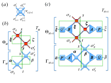
Figure 1: (Color online) (a) A single vertex in the QTM. (b) Configuration of the augmented system (environment) block $\Gamma_{M}$ ($\Theta_{M}$), where $\left\{\left|{\alpha}\right\rangle\right\}$ and $\left\{\left|{\beta}\right\rangle\right\}$ ($\left\{\left|{\xi}\right\rangle\right\}$ and $\left\{\left|{\zeta}\right\rangle\right\})$ represent the reduced dual biorthonormal bases of the current system (environment) block. The superblock $T_{M}$ is formed by contracting indices $s$, and $t$. (c) The enlarged augmented system (environment) block $\Gamma_{M+1}$ ($\Theta_{M+1})$ is obtained by adding one vertex and mapping it onto the new dual biorthonormal bases associated with $\left\{\left|\overline{\alpha}\right\rangle\right\}$ and $\left\{\left|\overline{\beta}\right\rangle\right\}$, obtained through renormalization of $T_{M}$.

The heart of the BTMRG is the bi-orthonormalization procedure for any two sets of arbitrary vectors $\left\{\left|a\right\rangle\right\}$ and $\left\{\left|b\right\rangle\right\}$, where $a,b=1,\cdots,m$. Let $A\equiv[\left|a\right\rangle]$ and $B\equiv[\left|b\right\rangle]$ be matrices with the vectors $\left|a\right\rangle$ and $\left|b\right\rangle$ as their columns. Performing a singular value decomposition (SVD) upon $A^{{\dagger}}B$ to obtain $A^{{\dagger}}B=U\Lambda V^{{\dagger}}$, we can readily obtain a dual set of biorthonormal bases $\widetilde{A}\equiv[\left|\alpha\right\rangle]=AP$ and $\widetilde{B}\equiv[\left|\beta\right\rangle]=BQ$, where $P=U\Lambda^{-1/2}$ and $Q=V\Lambda^{-1/2}$ represent non-unitary basis transformations. In the spirit of DMRG, as shown in Fig. 1(b), $T_{M}$ is partitioned into a system block and an environment block (enclosed in dashed frames) together with two additional time slices (labeled by $\sigma_{S}^{\phantom{\prime}}$, $\sigma_{S}^{\prime}$ and $\sigma_{E}^{\phantom{\prime}},\sigma_{E}^{\prime}$). At any step, we keep a dual set of biorthonormal bases for current system (environment) block labeled by $\left\{\left|\alpha\right\rangle\right\}$ and $\left\{\left|\beta\right\rangle\right\}$ ($\left\{\left|\xi\right\rangle\right\}$ and $\left\{\left|\zeta\right\rangle\right\}$) for the left and right dominant eigenvectors. Matrix elements of the augmented system block ${\Gamma}_{M}$ are obtained by projecting ${\Gamma}_{M}$ onto the dual biorthonormal bases associated with $\left\{\left|\alpha\right\rangle\right\}$ and $\left\{\left|\beta\right\rangle\right\}$ as ${\Gamma}_{M}(s{\alpha}\sigma_{S}^{\phantom{\prime}},\sigma_{E}^{\prime}{\beta}t)=\left\langle s{\alpha}\sigma_{S}\right|\Gamma_{M}\left|\sigma_{E}^{\prime}{\beta}t\right\rangle$, where $|\sigma_{E}^{\prime}\beta t\rangle\equiv|\sigma_{E}^{\prime}\rangle\otimes|\beta\rangle\otimes|t\rangle$, and similarly for the augmented environment block $\Theta_{M}$ onto the bases associated with $\left\{\left|{\xi}\right\rangle\right\}$ and $\left\{\left|{\zeta}\right\rangle\right\}$. In the case where the Hamiltonian has the reflection-symmetry ${h}_{i,i+1}={h}_{i+1,i}$, $\Theta_{M}$ is simply the reflection of ${\Gamma}_{M}$, ${\Theta}_{M}(\sigma_{E}^{\phantom{\prime}}{\xi}t,s{\zeta}\sigma_{S}^{\prime})={\Gamma}_{M}(s{\zeta}\sigma_{S}^{\prime},\sigma_{E}{\xi}t)$, such that only the augmented system block ${\Gamma}_{M}$ needs to be calculated and stored. The superblock $T_{M}$ is built by connecting ${\Gamma}_{M}$ and ${\Theta}_{M}$ through contracting the indices $s$ and $t$:

$$T_{M}(\xi\sigma_{E}\alpha\sigma_{S},\zeta\sigma_{E}^{\prime}\beta\sigma_{S}^{\prime})$$ (3)

$$= \underset{s,t}{\sum}{\Gamma}_{M}(s{\alpha}\sigma_{S},\sigma_{E}^{\prime}{\beta}t){\Theta}_{M}(\sigma_{E}{\xi}t,s{\zeta}\sigma_{S}^{\prime}).$$

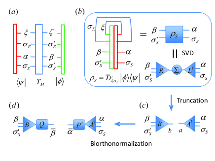
Figure 2: (Color online) Main steps of RG iteration in BTMRG. (a) Computation of the maximal eigenvalue and left and right eigenvectors $|\psi\rangle$, $|\phi\rangle$ of $T_{M}$. (b) The reduced density matrix $\rho_{s}$ is formed, using $|\psi\rangle$ and $|\phi\rangle$ and tracing out the environment. Performing SVD on $\rho_{s}$ and (c) keeping two reduced sets of basis vectors $\{|a\rangle\}$ and $\{|b\rangle\}$ from singular vectors of $\rho_{s}$ in $L$ and $R$. (d) The bases are biorthonormalized to form a new reduced dual biorthonormal bases $|\{\overline{\alpha}\rangle\}$ and $\{|\overline{\beta}\rangle\}$ for the new system block as in Fig. 1(c).

Figure 2 sketches the main steps of the renormalization group (RG) iteration in BTMRG. We first calculate the maximum eigenvalue and the right eigenvectors $\left|\phi\right\rangle$ of ${T}_{M}$ (Fig. 2(a)). The left eigenvector $\left|\psi\right\rangle$ can be directly read out from $\left|\phi\right\rangle$: $\psi_{{\xi}\sigma_{E}{\alpha}\sigma_{S}}=\phi_{{\beta}\sigma_{E}{\zeta}\sigma_{S}}$ Wang and Xiang (1997). No explicit construction of ${T}_{M}$ is required since only matrix-vector multiplication is involved in determining the maximum eigenvalue and eigenvectors, leading to a dramatic reduction of memory usage and computation time. The reduced biorthonormal bases $\{|\overline{\alpha}\rangle\}$ and $\{|\overline{\beta}\rangle\}$ for the new system block are determined from a non-Hermitian reduced density matrix ${\rho}_{S}=Tr_{\sigma_{E}\xi}\left|\phi\right\rangle\left\langle\psi\right|$ (Fig. 2(b)). By carrying out SVD upon $\rho_{S}=R\Sigma L^{{\dagger}}$, we keep two reduced sets of vectors $\left\{\left|a\right\rangle\right\}$ and $\left\{\left|b\right\rangle\right\}$ from singular vectors in $L$ and $R$ corresponding to the $m$ largest singular values in $\Sigma$ (Fig. 2(c)). Finally, we perform the prescribed biorthonormalization procedure to obtain the dual bases $\{|\overline{\alpha}\rangle\}$ and $\{|\overline{\beta}\rangle\}$. This process is equivalent to applying non-unitary basis transformations $P$ and $Q$ upon $\left\{\left|a\right\rangle\right\}$ and $\left\{\left|b\right\rangle\right\}$ (Fig. 2(d)). This completes a cycle of the RG steps in BTMRG. The augmented system block is enlarged by adding one vertex to $\Gamma_{M}$, and the enlarged Hilbert space is truncated by mapping back to the new reduced biorthonormal bases associated with $\{|\overline{\alpha}\rangle\}$ and $\{|\overline{\beta}\}$ (Fig. 1(c)). The next cycle is repeated with the new system block until the desired $M$ is reached.

Instead of performing SVD, conventional TMRG diagonalizes ${\rho}_{S}$ to obtain two reduced sets of left and right eigenvectors, which automatically satisfy the biorthonormal condition. The BTMRG makes clear this insight and generalizes the conventional TMRG to a broad class of biorthonormal bases. We note that the choices of the biorthonormal bases are not unique Huang (2011a); *YHuang2011b and the the steps proposed above are crucial in order to exploit symmetries of the Hamiltonian. The advantage of BTMRG over the conventional TMRG is now clear. In TMRG, the complete diagonalization of the non-Hermitian reduced density matrix will inevitably encounter the problem of complex eigenvalues and eigenvectors, and introduces numerical instability that prevents one from reaching very low temperatures. In BTMRG, on the other hand, only SVD is involved and we obtain real singular values and singular vectors. Note that the small singular values obtained during the biorthonormaliztion procedure can also induce instability to the BTMRG algorithm. But this can be remedied by replacing the dual corresponding basis vectors associated with the small singular value Huang (2011b).

We demonstrate the power of BTMRG using isotropic Heisenberg spin-$1/2$ chain whose Hamiltonian reads:

$${H}=\sum_{i=1}^{N}J\left({S}_{i}^{x}{S}_{i+1}^{x}+{S}_{i}^{y}{S}_{i+1}^{y}+{S}_{i}^{z}{S}_{i+1}^{z}\right),$$ (4)

The local Hamiltonian ${h}_{i,i+1}$ in Eq. (4) conserves total spin thus $q_{i}=\sum_{k}(-1)^{i+k}\sigma_{k}^{i}$ can be regarded as a good quantum number of the QTM Wang and Xiang (1997). Consequently both $T_{M}$ and the reduced density matrix $\rho_{S}$ are block-diagonal and the SVD and the biorthonormalization can both be carried out independently for each subblock for different $q_{i}$. In addition, the maximum eigenvalue occurs in the subblock labeled by $q_{i}=0$ Nomura and Yamada (1991), which results in further simplification. The Helmholtz free energy in the thermodynamic limit can be calculated from the maximum eigenvalue $\Lambda_{0}$ of ${T}_{M}$ as

$$f=-T\underset{N\rightarrow\infty}{\lim}\frac{\log(Z)}{N}=-\frac{T}{2}\log\Lambda_{0}.$$ (5)

Other thermodynamics quantities can either be calculated from the numerical derivatives of the free energy or directly using the dominant eigenvectors and eigenvalues of the QTM. Systematic errors come from two sources: the finiteness of the imaginary-time step $\varepsilon$, and truncation of the reduced basis set. In principle, the first source of error has a $O(\varepsilon^{2})$ correction in the partition function. In practice we find that $\varepsilon=0.05$ is adequate for the models studied in this work. On the other hand, the truncation error can be estimated by the discarded weight $w_{d}=1-\sum_{i=1}^{m}\lambda_{i}$, where $\lambda_{i}$’s are the singular values in the SVD of the reduced density matrix $\rho_{s}$ and $m$ is the number of basis states kept by BTMRG. In this work, we fixed the discarded weight to be $w_{d}=10^{-20}$ and set up a maximum number of basis states $m$ which leads to a fast computation in the first several hundred iterations of the RG steps.

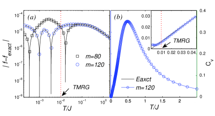
Figure 3: (Color online) (a) Deviations of the BTMRG free energy from the exact results for the isotropic Heisenberg model down to temperature $T/J=0.0002$ for both $m=80$ and $120$. (b) BTMRG and exact results for the specific heat $C_{v}$. Inset: Low temperature regime where the exact results is $C_{v}=(2/3)T$. The TMRG arrows indicate the typical temperature reachable by conventional TMRG.

In Fig. 3(a) we plot the deviation of the BTMRG results with $m=80$ and $120$ from the solution based on the Bethe ansatz Klümper (1993, 2004). We find that the BTMRG is very stable and can reach temperature down to $T/J=0.0002$ for both $m$’s. For a similar $m$, conventional TMRG can only reach down to $T/J=0.01$ due to the numerical instability. Furthermore, we note that $T/J=0.0002$ is not yet the limit of our algorithm, and even lower temperature can be reached by continuing the RG iteration before eventually the numerical instability sets in. More importantly, the accuracy is competitive with the conventional TMRG down to temperature $T/J=0.01$ Sirker (2002), and the absolute error remains within the order of $10^{-5}$ down to $T/J=0.0002$. At low temperatures the truncation error dominates and higher accuracy can be reached by keeping more states, which is clearly shown in Fig. 3. At high temperatures, the Trotter error due to the finite imaginary time step dominates. Due to the small length of the QTM, the number of states kept by BTMRG to keep the discarded weight $w_{d}=10^{-20}$ may not reach the cutoff $m$. Consequently, the accuracy is less sensitive to $m$. Since the calculation is not variational, the numerical results might be larger or smaller than exact values, and an zero error crossing will give rise to the cusps in the error curve. In Fig. 3(b) we show the results of the specific heat $C_{v}$, and an excellent agreement with the exact result is obtained. In the inset, we zoom into the low temperature regime where the exact result is $C_{v}=(2/3)T$ Bursill et al. (1996); *XWang1997. The BTMRG results start to deviate from the exact value at a much lower temperature compared to conventional TMRG. The deviation is due to accumulation of truncation error and not the numerical instability.

To examine the scalability of BTMRG, we also study the 1D frustrated $J_{1}$-$J_{2}$ model with the Hamitonian:

$$H=\sum_{i=1}^{N}J_{1}\vec{S}_{i}\cdot\vec{S}_{i+1}+J_{2}\vec{S}_{i}\cdot\vec{S}_{i+2}.$$ (6)

We consider the case of ferromagnetic nearest-neighbor (NN) interaction $(J_{1}=-1)$ and antiferromagnetic next-nearest-neighbor (NNN) interaction $(J_{2}=0.4)$. We block two adjacent spins as a superspin to obtain a new local Hamiltonian with only NN interaction. Moreover, the QTM of this model possesses neither reflection symmetry nor conserved quantum numbers, which makes the computation much more numerically demanding. In Fig. 4 we calculate the specific heat $C_{v}$ down to temperature $T/|J_{1}|=0.003$ for $m=80$ and $120$. We find a sharp low-temperature anomaly and a broad shoulder at higher temperatures which are in good agreement with the results of conventional TMRG Lu et al. (2006). In the inset of Fig. 4 the low-temperature behavior is magnified. We observe an inflection of the $C_{v}$ curve at very low-temperature. For larger $m$ the $C_{v}$ starts to inflect at lower temperature, indicating the inflection is due to the accumulation of truncation error and not the numerical stability. By increasing the value of $m$, the BTMRG can still be accurately pushed to far lower temperature unreachable by TMRG without suffering from numerical instability.

Our BTMRG computations were performed by using Matlab on a laptop with an Intel Core i5@ 2.3GHz CPU and 4G RAM. It takes about five days to generate a supperblock with size $2M=2\cdot 10^{5}$ for $m=120$. Since BTMRG does not involve complicated eigenvalue decomposition of the non-Hermitian $\rho_{s}$ as in conventional TMRG, no special numerical tricks are necessary, and the computational complexity is significantly reduced.

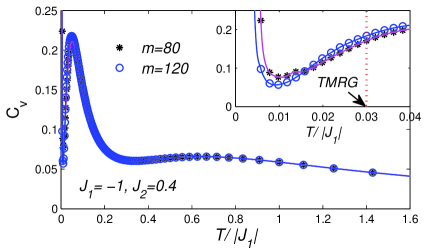
Figure 4: (Color online) Specific heat $C_{v}$ as a function of the temperature for the $J_{1}$-$J_{2}$ model down to temperature $T/|J_{1}|=0.003$. Inset: The inflection of the $C_{v}$ near below $T/|J_{1}|=0.01$ is a result of accumulation of truncation error.

In summary, we apply BTMRG method to accurately determine the thermodynamic properties of 1D quantum spin chains at low temperatures. Due to the improved numerical stability of the BTMRG, the simulations can access temperatures several orders of magnitude lower than the conventional TMRG, while retaining the same level of accuracy. This work suggests that the BTMRG is a promising numerical method to investigate the low temperature thermodynamics of Q1D quantum systems. For example, it may become possible to study the behavior near a quantum critical point, the transition from high-temperature regime into the quantum critical regime, and make direct comparison with experiments. In addition it may also be possible to extend the long-time limit in the studies of real-time dynamics Sirker and Klümper (2005).