First principle electronic, structural, elastic, and optical properties of strontium titanate

Abstract

We report self-consistent ab-initio electronic, structural, elastic, and optical properties of cubic SrTiO₃ perovskite. Our non-relativistic calculations employed a generalized gradient approximation (GGA) potential and the linear combination of atomic orbitals (LCAO) formalism. The distinctive feature of our computations stem from solving self-consistently the system of equations describing the GGA, using the Bagayoko-Zhao-Williams (BZW) method. Our results are in agreement with experimental ones where the later are available. In particular, our theoretical, indirect band gap of 3.24 eV, at the experimental lattice constant of 3.91 Å, is in excellent agreement with experiment. Our predicted, equilibrium lattice constant is 3.92 Å, with a corresponding indirect band gap of 3.21 eV and bulk modulus of 183 GPa.

I Introduction

Strontium titanate (SrTiO₃) is one of the most studied oxides of the ABO₃ perovskite type structures, due to its great technological importance. Many interesting phenomena such as colossal magnetoresistance, high-$T_{c}$ superconductivity, multiferroicity, and ferroelectricity are observed in complex oxides. Since most of the interesting complex oxides have perovskite structure, SrTiO₃ is an ideal starting point for their study. It has been widely used for integration with other oxides into heterostructures. Those heterostructres show interesting properties such as thermoelectricityOhta et al. (2007); Wunderlich et al. (2009) and superconductivityCaviglia et al. (2008); Chang et al. (2010). Many new concepts of modern condensed matter and the physics of phase transitions have been developed while investigating this unique materialHeifets et al. (2006); Wang et al. (2001); Lines and Glass (1997). SrTiO₃ has applications in the fields of ferroelectricity, optoelectronics and macroelectronics. It is used as a substrate for the epitaxial growth of high temperature superconductors. SrTiO₃ exhibits a very large dielectric constant. In comparison with SiO₂, SrTiO₃ has almost two orders of magnitude higher dielectric constant and may as well offer a better replacement for SiO₂ in Si-based nanoelectronic devices (see Wilk et al. (2001)[and references therein]). SrTiO₃ has found usage in optical switches, grain-boundary barrier layer capacitors, catalytic activators, waveguides, laser frequency doubling, high capacity computer memory cells, oxygen gas sensors, semiconductivity, etc Eglitis et al. (2004); Piskunov et al. (2004); Tinte et al. (1998); Jiangni et al. (2006); Cai and Zhang (2004); Bednorz and Muller (1984); Balachandran and Eror (1981); Kim et al. (1985).

During the last few decades, the electronic, structural, elastic, and optical properties of SrTiO₃ (STO), as a model of ABO₃ perovskite, have been under intensive investigation both experimentallyBickel et al. (1989); Maus-Friedrichs et al. (2002); Charlton et al. (2000); Ikeda et al. (1999); Reihl et al. (1984); Pertosa and Michel-Calendini (1978); Brookes et al. (1986) and theoretically Eglitis et al. (2004); Piskunov et al. (2004); Tinte et al. (1998); Jiangni et al. (2006); Cai and Zhang (2004); Padilla and Vanderbilt (1997, 1998); Cheng et al. (2000); Tinte and Stachiotti (2000). But, from a theoretical point of view, a proper description of its electronic properties is still an area of active research. Theoretical computations have had difficulty in predicting the correct band gap energy and other related electronic properties of SrTiO₃ from first principle. The density functional theory plus additional Couloumb interactions (DFT+U) formalism Anisimov et al. (1991); Anisimov and Gunnarsson (1991); Anisimov et al. (1997); Madsen and Novák (2005) has had good successes in obtaining correct energy bands and gaps of materials, but can only be applied to correlated and localized electrons, e.g., 3d or 4f in transition and rare-earth oxides. The hybrid functionals (for e.g., Heyd-Scuseria-Ernzerhof (HSE) hybrid functional Heyd et al. (2006, 2004, 2003)) has also been used in attempt to improve on the energy bands and band gaps of materials. This approach involves a range separation of the exchange energy into some fraction of nonlocal Hartree-Fock exchange potential and a fraction of local spin density approximation (LSDA) or generalized gradient approximation (GGA) exchange potential. We should note that this range separation is not universal. There is always a range separation parameter $\omega$ which varies between 0 and $\infty$. While it is reasonably clear that there exists a value of $\omega$ that gives the correct gap for a given system, this $\omega$ is not universal as it is always adjusted from one system to another Paier et al. (2008); Henderson et al. (20011). For example, in HSE06 Heyd et al. (2006); Krukau et al. (2006), $\omega$ $=$ 0.11$a_{0}^{-1}$ ($a_{0}$ is the Bohr radius) and in Perdew-Burke-Ernzerhof (PBEh) global hybrid Janesko et al. (2008), it is 25 $\%$ short-range exact exchange and 75 $\%$ short-range PBE exchange. Even though the HSE functional, in most cases, accurately reproduces the optical gap in semiconductors, it severely underestimates the gap in insulators Henderson et al. (20011); Stroppa et al. (2007) and its band width in metallic systems is generally too large Henderson et al. (20011); Stroppa et al. (2007); Paier et al. (2006); Koller et al. (2011). The Engel and Vosko (1993) (EV) GGA and the  Tran and Blaha Tran and Blaha (2009) modified Becke-Johnson (TB-mBJ) have also provided some improvements to the band gap of materials. For TB-mBJ, while the band gaps are considerably improved, the effective masses are severely underestimated Koller et al. (2011). In the case of the EV potential, the equilibrium lattice constants are far too large as compared to experiment and, as such, leads to an unsatisfactory total energy Dufek et al. (1994); Singh (2010).

The theoretical underestimations of band gaps and other energy eigenvalues have been ascribed to the inadequacies of density functional potentials for the description of ground state electronic properties of semiconductors Maus-Friedrichs et al. (2002); Charlton et al. (2000); Padilla and Vanderbilt (1997). Also, other methods Chan and Ceder (2010); Georges et al. (1996); Bechstedt et al. (2009) that entirely go beyond the density functional theory (DFT) do not obtain the correct band gap values of most semiconductors without adjustment or fitting parameters Kim and Park (2010); Ahn et al. (2006). This unsatisfactory situation is a key motivation for our work.

Stoichiometric STO has an experimental, indirect band gap of 3.20 - 3.25 eV at room temperature Bickel et al. (1989); Charlton et al. (2000); Ikeda et al. (1999). Theoretical calculations using several techniques have led to band gaps of SrTiO₃ in the ranges 1.71 to 2.2 eV for LDA and GGA Wang et al. (2001); Piskunov et al. (2004); Jiangni et al. (2006), 1.87 to 3.63 eV for Hybrid DFT Heifets et al. (2006); Eglitis et al. (2004); Piskunov et al. (2004), and value as high as 11.97 eV for the Hatree-Fock (HF) method Piskunov et al. (2004).

In this paper, we present a simple, yet robust, and ab-initio method, based on self consistent solutions of the pertinent system of equations Zhao et al. (1999); Bagayoko et al. (2007); Ekuma et al. (2011a); Bagayoko and Franklin (2005), that correctly predicts band gap values and related electronic properties of SrTiO₃ rigorously, from first principle, within the LCAO-GGA formalism. We also compute the structural, elastic and optical properties of SrTiO₃.

The rest of this article is organized as follows. After this introduction in section  I, the computational methods and details are given in section  II. The results of our self-consistent calculations are presented and discussed in section  III. We then summarize and conclude in section  IV.

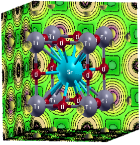
Figure 1: (Color online). The iso-surface cubic unit cell of SrTiO₃ with the iso-lines, at lattice parameter of 3.91 Å.

II Methods and Computational Details

In the ground state, STO has the simple cubic (O${}_{h}^{1}$ - Pm$\bar{3}$m) perovskite structureICSD (2011), with Sr atom sitting at the origin, Ti at the body center and three oxygen atoms at the three face centers Wyckoff (1963) (see Fig. 1). We used the room temperature experimental lattice constant of 3.91 Å ICSD (2011); Wyckoff (1963).

Figure 2: Calculated, band structure of c-SrTiO₃ at the experimental lattice constant of 3.91 Å as obtained with the optimal basis set using PW - GGA. The horizontal, dashed line indicates the position of the Fermi energy (E_F) (-0.10872 eV) which has been set equal to zero.

Our ab initio, self consistent, nonrelativistic calculations employed a linear combination of atomic orbitals (LCAO) formalism and a generalized gradient approximation (GGA) potential. One may argue that relativistic effects are important for the description of SrTiO₃. As was noted by  Marques et al. Marques et al. (2003), relativistic effects are only important for the description of the high-$\kappa$ dielectric band structure. Their calculated, relativistic and non-relativistic band structure for SrTiO₃, up to an energy of 5 eV for the valence and conduction bands, respectively, are almost identical. Consequently, we expect a negligible relativistic correction for the band gap of SrTiO₃.

The distinctive feature of our calculations, the use of the Bagayoko, Zhao, and Williams (BZW) method, has been extensively described in the literature Zhao et al. (1999); Bagayoko et al. (2007); Ekuma (2010); Ekuma et al. (2011a); Bagayoko and Franklin (2005); Ekuma and Bagayoko (2011); Bagayoko et al. (2004). This method has been shown to lead to accurate ground state properties of many semiconductors: c-InN Bagayoko et al. (2004), w-InN Bagayoko and Franklin (2005), w-CdS Ekuma et al. (2011a), c-CdS Ekuma et al. (2011b), rutile-TiO₂ Ekuma and Bagayoko (2011), AlAs Jin et al. (2006), GaN, Si, C, RuO₂ Zhao et al. (1999), and carbon nanotubes Zhao et al. (2004).

Instead of assuming that a single trial basis set will yield the correct ground state charge density of the solid, the BZW method entails a minimum of three self-consistent calculations with basis sets of different sizes and generally with different polarization functions, i.e., p, d, and f functions. The correct ground state is the one where all the occupied energies are at their minima. In practice, up to seven self-consistent calculations have been performed for some materials e.g, wurtzite ZnO Franklin et al. (20xx). The computations begin with a relatively small basis set that should not be smaller than the minimal basis set. The latter is defined as one that is just large enough to account for all the electrons in the atomic or ionic species present in the solid. The preliminary, self-consistent calculations of the electronic properties of the species provide the wave functions that serve as input in the solid state calculations.

The first, self consistent calculation for the solid is performed with this small basis set (Calculation I) that is subsequently augmented with one orbital for the next self-consistent calculation (Calculation II). Depending on the angular symmetry of the added orbital, the size of the new basis set is larger than that of the previous one by 2, 6, 10, or 14 for $s$, $p$, $d$, and f functions, respectively. The occupied energies from calculations I and II are compared graphically and numerically. For the first two calculations, we found these occupied energies to be different for all the solids we have studied to date Ekuma et al. (2011c); Bagayoko (2008), including SrTiO₃. The basis set for calculation II is then augmented in order to carry out self-consistent calculation III. Again, the occupied energies from calculations II and III are compared. This process of augmenting the basis set and of performing self-consistent calculations is continued until the occupied energies from a calculation, say N, are found to be identical to their corresponding ones from calculation (N+1), within computational uncertainties that are less than 50 meV. This perfect superposition of occupied energies from two consecutive calculations identifies the basis set for Calculation N as the optimal one, i.e, the smallest basis set that yields the lowest, occupied energies of the system. The attainement of this minima signifies that this basis set is verifiably complete for the description of the ground state of the system. Larger basis sets that include the optimal one do not lower any occupied energies from their values obtained with the optimal basis set.

As explained elsewhere Ekuma et al. (2011a); Zhao et al. (1999), these larger basis sets do not lead to any changes in the ground state charge density or the Hamiltonian. However, larger basis sets that include the optimal one often lead to a lowering of some unoccupied energies. This lowering of some unoccupied energies cannot be ascribed to a physical interaction included in the Hamiltonian. Up to the optimal basis set, changes in the basis sets lead to changes in the charge density, the potential, and the Hamiltonian. Hence, changes in occupied and unoccupied energies, for self-consistent calculations with basis sets up to the optimal one, can be ascribed to a physical interaction embedded in the Kohn-Sham Hamiltonian. The system of equations in DFT totally determines changes in the occupied states. It also determines, at least in part, low-laying unoccupied states that are interacting with the occupied ones, up to the optimal basis set. For example, in wurtzite InN, the calculated dielectric functions agree with their corresponding experimental ones up to 5.5-6.0 eV Jin et al. (2007). Given that only direct transitions were taken into account in our dielectric functions calculations, this agreement indicates that the low-laying unoccupied bands were correctly determined. For larger basis sets that include the optimal one, the extra lowering of some unoccupied energies is a direct consequence of the Rayleigh theorem Ekuma (2010); Ekuma et al. (2011a); Ekuma and Bagayoko (2011); Ekuma et al. (2011c). This theorem states that when an eigenvalue equation is solved with basis sets I and II, with set II larger than I and including I entirely, then the eigenvalues obtained with set II are lower than or equal to their corresponding ones obtained with basis set I Ekuma et al. (2011a); Ekuma and Bagayoko (2011).

The above process entails iterations for the equation giving the ground state charge density, with the iterations for the Kohn-Sham equation carried out for each choice of the basis set. Given that iterations for the Kohn-Sham (KS) equation involves the charge density (CD) equation, one could conclude that a single trial basis set calculation solves both equations self consistently. A problem with this view stems from the fact that any two such calculations, with different trial basis sets, lead to different, converged (i.e., self consistent) eigenvalues of the KS equation. The fundamental theorem of algebra suffices to guarantee that the two sets will be different if the basis sets have different numbers of basis functions utilized in the expansions. The question then arises as to which of the two sets of eigenvalues of the KS equation provides the physical description of the system under study. To answer such a question definitively and from first principle, the BZW method follows the process described above. Upon reaching the optimal basis set, not only the charge density, the potential, and the Hamiltonian no longer change (i.e., they have converged), but also the resulting, self-consistent eigenvalues of the KS equation have reached their respective minima, for the occupied states. In our understanding, to solve the system of equation self-consistently means obtaining converged eigenvalues (attainable with most arbitrary basis set) but also occupied eigenvalues that have reached their respective minima (attainable with BZW method).

In the above sense, the BZW method solves self-consistently not just the Kohn-Sham equation, but also the equation giving the ground state charge density in terms of the wave functions of the occupied states. Further, in his Nobel lecture Kohn (1999), Kohn noted the “density optimal” feature of the wave functions from correctly performed DFT calculations while those for the Hartree Fock approach are “total-energy optimal.” Without a constrained search for the converged ground state, it is quite difficult to infer the basis set that yields the correct ground state charge density Levy (1982, 1979). This point becomes clearer by noting that the reorganization of the cloud of valence electrons is drastically different for atomic or ionic species as compared to molecules or solids. For instance, single trial basis set calculations cannot make up for any deficiency in the angular symmetry of the functions, irrespective of the degree of convergence of the iterations of the Kohn-Sham equation. By correct ground state charge density, we mean the charge density that leads to the minima of all the occupied energies.

In this work, we utilize the electronic structure package from the Ames Laboratory of the US Department of Energy (DOE), Ames, Iowa Harmon et al. (1982). We employ the generalized gradient approximation (GGA) potential given by  Perdew and Wang Perdew and Wang (1992). We utilize sets of even tempered Gaussian functions with exponents from 0.12 to 10⁵ to form the atomic wavefunctions. There are 15, 15, and 13 s, p, and d orbitals, respectively, for Sr, while 17, 17, and 15 s, p, and d orbitals, respectively, are used for both Ti and O. The charge fitting error using the Gaussian functions in the atomic calculation is about 10^-4. Since the deep core states are fully occupied and are inactive chemically, the charge densities of the deep core states were kept the same as in the free atom. However, the core states of low binding energy were still allowed to fully relax, along with the valence states, in the self consistent calculations. The orbitals employed in the self-consistent calculations are between paranthesis for Sr (3d 4s 4p 4d 5s), Ti (3p 3d 4s) and O (2s 2p 3s), including some that are unoccupied in the free atoms or ions. These unoccupied orbitals are included in the self-consistent LCAO calculation to allow the restructuring of the electronic cloud, including possible polarization, in the crystal environment.

The Brillouin zone (BZ) integration for the charge density in the self consistent procedure is based on 56 special k points in the irreducible Brillouin zone (IBZ). The computational error for the valence charge is 5.3 x 10^-5 eV per valence electron. The self consistent potential converged to a difference of 10^-5 after several tenths of iterations. The energy eigenvalues and eigenfunctions are then solved at 161 special k points in the IBZ for the band structure. A total of 152 weighted k points, chosen along the high symmetry lines in the IBZ of SrTiO₃, are used to solve for the energy eigenvalues from which the electron density of states (DOS) are calculated using the linear analytical tetrahedron method Lehmann and Taut (1972). The partial density of states (pDOS) and the effective charge at each atomic sites are evaluated using the Mulliken charge analysis procedure Mulliken (1955). We also calculated, the equilibrium lattice constant $a_{o}$, the bulk modulus ($B_{o}$), the associated total energy and the electron and hole effective masses in different directions.

In calculating the lattice constant, we utilize a least square fit of our data to the Murnaghan’s equation of state Murnaghan (1944); Mur (1995). The lattice constant for the minimum total energy is the equilibrium one. The bulk modulus ($B_{o}$) is calculated at the equilibrium lattice constant.

The dielectric function $\varepsilon(\omega)=\varepsilon_{1}(\omega)+i\varepsilon_{2}(\omega)$ can be calculated once the electronic wave functions and energies are known. The imaginary part of the dielectric function $\varepsilon_{2}(\omega)$, from the direct interband transitions, is calculated using the Kubo-Greenwood formula Bocquet et al. (1996):

$$\varepsilon_{2}(\omega)=\frac{8\pi^{2}e^{2}}{3m^{2}\hbar\omega^{2}\Omega}\sum_{k}\sum_{nl}|\langle\psi_{kn}(r)|P|\psi_{kl}(r)\rangle|^{2}f_{kl}[1-f_{kn}]\delta(\epsilon_{kn}-\epsilon_{kl}-\hbar\omega)$$ (1)

where $\hbar\omega$ is the photon energy, $P$ = $-i\hbar\triangledown$ is the momentum operator, $\Omega$ is the volume of the unit cell, $\psi_{kn}(r)$ and $\psi_{kl}(r)$ are the initial and final states, respectively, $f_{ki}$ is the Fermi distribution function for the $i_{th}$ states, and $\epsilon_{ki}$ is the energy of the electron in the $i_{th}$ state. The real part of the dielectric function, $\varepsilon_{1}(\omega)$, is obtained from the well-known Kramers-Kronig (KK) relation,

$$\varepsilon_{1}(\omega)=1+\frac{2}{\pi}M\int_{0}^{\infty}\frac{\varepsilon_{2}(\omega^{\prime})\omega^{\prime}}{\omega^{\prime 2}-\omega^{2}}d\omega^{\prime},$$ (2)

where $M$ indicates the principal value of the integral Ching (1990). The real part of the optical conductivity, $Re[\sigma(\omega)]$, follows from above as

$$Re[\sigma(\omega)])={\frac{\omega}{4\pi}}\varepsilon_{2}(\omega)$$ (3)

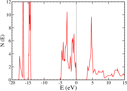
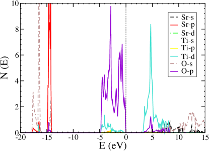
Figure 3: (Color online). (a) Calculated, density of states (DOS) of c-SrTiO₃ at the experimental lattice constant of 3.91 Å as obtained with the optimal basis set using PW - GGA. (b) Calculated, partial density of states (pDOS) of c-SrTiO₃ at the experimental lattice constant of 3.91 Å as obtained with the optimal basis set using PW - GGA. The vertical, dashed line indicates the position of the Fermi energy (E_F) which has been set equal to zero.

III Results and Discussion

The results of the electronic structure computations are given in Figs. 2 to 4. Figure  5 depicts the calculated total energy of STO, while Fig. 6 shows the optical spectra obtained using the optimal basis set from the electronic structure computations. Figures 1 and 4 have been drawn using the xcrysden Kokalj (2003). We discuss the electronic structure, low laying conduction bands, and the effective mass in  III.1. The DOS is discussed elaborately in III.2. The structural properties are presented in III.3, while III.4 deals with the calculated, optical properties.

III.1 The Electronic Structure, Band Gap, Low-energy Conduction Band and Effective Mass

The electronic structure of the valence and the low energy conduction states determine the band gap and other important properties of materials. Table 1 shows that our ab initio, first principle method yielded an indirect band gap of 3.24 eV at the experimental lattice constant of 3.91 Å (see Fig. 2) and an indirect band gap of 3.21 eV at the calculated equilibrium lattice constant of 3.92 Å. This table contains several, previous results from calculations using LDA, GGA or hybrid potentials. Table 2 contains the calculated energies at some high symmetry points in the BZ. These energies are provided for future comparison with experimental and theoretical findings. Our calculated band structure (see Fig. 2) resembles that of the parent TiO₂ system. Fig. 2 also shows that the top of the valence band is at the $L$ point.

The effective mass is one of the main factors determining the transport properties, the Seebeck coefficient, and electrical conductivity of materials. The calculated electron effective masses at the bottom of the conduction band along the $\Gamma$ - $L$, $\Gamma$ - $X$, and $\Gamma$ - $K$ directions, respectively, are 0.68 - 0.81, 0.44 - 0.59, and 0.51 - 0.66 while the calculated hole effective masses at the top of the valence band, along the $\Gamma$ - $L$, $\Gamma$ - $X$, and $\Gamma$ - $K$ directions, respectively, are 0.64 - 0.83, 1.22 - 1.27, and 0.96 - 1.02 (all in units of the electron mass). The observed anisotropy and the ranges of effective masses confirmed the earlier observations of Mattheiss and co-workers Mattheiss (1972a, b). Our calculated effective masses are in excellent agreement with the detailed effective mass values as reported by Mattheiss (1972a)[and references therein] and the relativistic computational results of  Marques et al. Marques et al. (2003).

Table 1: Comparison of our calculated band gap values with other theoretical and experimental ones, for c-SrTiO₃. Our calculations show that c-SrTiO₃ has an indirect band gap from $L$ to $\Gamma$ points. Exactly the same band gap value is found from $L$ to $X$ points. All the band gaps are indirect unless otherwise indicated with (D).

	Computational Method	Eg (eV)
GGA	GGA - BZW (Present work)	3.24
	(with equilibrium lattice constant)	3.21
	PP - PWGA	1.97
	PP - PBE	1.99
	FP - LAPW	1.80
	PP	1.60
	FLAPW	1.78
	TB - LMTO	1.40 (D)
	FB - LMTO	2.20 (D)
LDA	PP	2.04
	PP - PW	1.79
	LMTO - ASA	1.80
	PP	1.71
	PP - PW	1.79
	OLCAO	1.45
HF	PP	11.97
Hybrid DFT	B3PW - LCAO	3.63
	PP - BLYP	1.94
	PP - B3LYP	3.57
	PP - P3PW	3.63
	LCGO - B3PW	3.70
SA	FP - LAPW	1.87 - 3.25
Experiment	NA	3.10 - 3.25

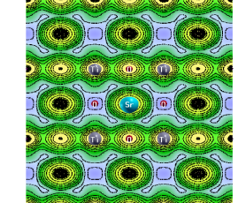
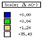
Figure 4: (Color online). The contour plot of the electron charge density of c-SrTiO₃ as obtained with the optimal basis set using PW - GGA. The center atom is Sr with Ti atoms at the corners and O atoms in the middle of the size of the parallelogram around Sr. $\Delta$ $n(r)$ is the variation of the electron charge density as a function of distance away from an atomic site. A logarithmic scale has been used.

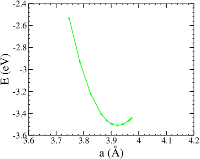
Figure 5: (Color online) Calculated, total energy per unit cell as a function of the lattice constant of c-SrTiO₃, as obtained with the optimal basis set using PW - GGA. The calculated equilibrium lattice constant is 3.92 Å.

There is a significant O_2p – Ti_3d hybridization in the valence bands. As shown in Fig. 2, the valence bands of SrTiO₃ can be divided into three distinct groups: the upper, intermediate, and lower groups of valence bands occupy the energy ranges of 0 to -5.80 eV, -14.2 to -14.78, and -16.62 to -17.80 eV, respectively. The upper VB bands are made up of nine bands with a bandwidth of 5.80 eV, in agreement with X-ray photoemission spectroscopy (XPS) values of 5 - 6 eV Zollner et al. (2000) and the GGA results of  Jiangni et al. Jiangni et al. (2006). They are formed by the hybridization between O 2p and Ti 3d, with very little contribution from the Ti 3p and Sr 4p (see Fig. 3(b)). Two of the bands at the $\Gamma$ point are triply degenerate: ${}^{1}{\Gamma}_{15}$ (-2.75 eV) and ${}^{2}\Gamma_{15}$ (-0.25 eV), while the third band $\Gamma_{25}$ (-1.23 eV) is non-degenerate (see Table 2). Immediately below the upper VB, a group of triply degenerate bands emanating from the hybridization between Sr 4p, O 2s and O 2p, with little dispersion at ${}^{3}\Gamma_{15}$. This group is located at -14.78 eV. The lowest lying VB bands are semi core like bands formed mainly due to the hybridization between O 2s, and Sr 4p with very little bonding coming from Ti 4s and Ti 3p. They are located at ${}^{1}\Gamma_{1}$ (-17.80 eV) and ${}^{2}\Gamma_{1}$ (-16.62 eV). Our calculated position of Sr 4p between - 14.78 to - 17.80 eV is in agreement with the XPS measurement of Battye et al. (1976) which placed it at 16.50 eV below the Fermi surface (E_F). Also, Board et al. (1970) and Battye et al. (1976) measured the average position of the O 2s to be about 17 eV below E_F. Our calculated value of -17.85 eV in Fig. 3(a) is close to the experimental one. In particular, our result does not underestimate this core state position as is often the case in GGA calculations.

The conduction bands (CB), immediately above the Fermi level (low energy conduction band), are dominated by threefold degenerate Ti 3d $t_{2g}$ orbitals which hybridize with O 2p and O 2s. The two-fold degenerate Ti 3d $e_{g}$ states have some hybridization from all other orbitals except Ti (4s and 3p), Sr (4p and 3d). The energy eigenvalue in the lowest conduction bands, at the $X$ point, are practically the same as that at the $\Gamma$ point, resulting in the observed, minimal dispersion in the conduction band between $\Gamma$ and $X$ points. This feature is apparent from our energies at the high symmetry points in Table II. At the $\Gamma$ point, energies associated with the lowest-laying conduction bands are: ${}^{1}\Gamma_{25^{\prime}}$ (3.24 eV), ${}^{1}\Gamma_{12}$ (4.84 eV), ${}^{2}\Gamma_{12}$ (6.10 eV), ${}^{3}\Gamma_{1}$ (6.75 eV) and ${}^{2}\Gamma_{25^{\prime}}$ (8.92 eV). The calculated, low energy conduction bands in Fig. 2 are quite different from those of previous studies. Figure 2 shows that the lowest conduction bands are degenerate at the $\Gamma$ and $X$ points along the [100] and equivalent directions. The electronic structure in Fig. 2 was calculated using the experimental lattice constant. We further examined whether or not the position of the shallow minimum in the lowest conduction band depends on the value of the lattice constant by using several values of the lattice constant around the experimental one. Even though, the band gap value changed from 3.26 to 3.17 eV, there was no appreciable change in the depth of the shallow minimum in the lowest conduction band. We recall that the gap is 3.21 eV for our calculated, equilibrium lattice parameter.

Table 2: Eigenvalues (eV), along high symmetry points, for c-SrTiO₃, as obtained with the experimental lattice constant of 3.91 Å. The Fermi energy of - 0.12188 eV is set to zero in the table. The energy eigenvalues at $\Gamma$ and $X$ points are found to be almost identical.

$L$	$\Gamma$	$X$	$K$
-32.06	-32.03	-32.03	-32.07
-32.06	-32.03	-32.03	-32.04
-32.06	-32.03	-32.03	-32.03
-16.19	-16.62	-16.62	-16.65
-16.19	-16.62	-16.62	-16.49
-14.96	-14.67	-14.67	-14.61
-14.96	-14.67	-14.67	-14.47
-14.96	-14.67	-14.67	-14.33
-4.94	-2.75	-2.75	-3.92
-4.32	-2.75	-2.75	-3.43
-4.32	-2.75	-2.75	-3.09
-3.58	-1.23	-1.23	-1.68
0	-0.25	-0.25	-1.33
0	-0.25	-0.25	-1.04
0	-0.25	-0.25	-0.73
5.22	3.24	3.24	4.06
5.22	3.24	3.24	4.12
5.22	3.24	3.24	4.33
8.65	4.82	4.82	5.38
10.92	10.28	10.28	13.42
10.92	10.28	10.28	14.47

Table 3: Experimental and theoretical lattice constants a (in Å) for c-SrTiO₃ along with the calculated values of the bulk modulus (in GPa).

	Computational Method	a (Å)	B (GPa)
GGA	BZW - LCAO (Present work)	3.92	183.45
	PP - PWGA	3.95 (3.93)	167 (195)
	PP - PBE	3.94 (3.93)	169 (195)
	PW	3.95 (3.88)	167 (194)
	PBE	3.95	167 (194)
	”	3.91 (3.82)	210.21 (252.92)
LDA	PP	3.86	214 (215)
	LAPW	3.86	204 (176)
	FLAPW	3.95	167
	”	3.93 (3.87)	207.28 (227.63)
	PP - PW	3.87	194
	OLCAO	3.93	163
HF	PP	3.92 (3.93)	219 (211)
	PP	3.98 (3.92)	208.85 (206.68)
Hybrid DFT	PP - BLYP	3.98	164
	PP - B3LYP	3.94	177 (187)
	PP - P3PW	3.90 (3.91)	177 (186)
Experiment	NA	3.89 - 3.92	174 - 183

III.2 Densities of States, Electron Distribution and Chemical Bonding

Figures 3(a) and 3(b) exhibit the total (DOS) and related partial (pDOS) densities of states, respectively. Figure 4 shows the contour plot of the distribution of the electron charge density of SrTiO₃. As can be seen from Fig. 4, the electron density of SrTiO₃, away from the atomic sites, does not have a spherically symmetric distribution. Further, the bonding between Ti and O is covalent, due to Ti-3$d$ and O-2$p$ hybridization, unlike in the case of Sr and O that is ionic. The bond length of Sr – O is 2.76 Å, with a minimum charge density of $\sim$ 0.19 $e$/ų, while Ti – O bond length is 1.95 Å, with a charge density of $\sim$ 0.63 $e$/ų. The experimental bond lengths for Sr – O and Ti – O are 2.76 and 1.96 Å, respectively, Kuroiwa et al. (2003); Jauch and Reehuis (2005) with corresponding charge densities of 0.2 and 0.67 – 0.90 $e$/ų, in that order Ikeda et al. (1998); Friis et al. (2004); Jauch and Reehuis (2005); Kuroiwa et al. (2003). The charge density distribution around the O atom with respect to the horizontal Ti – O – Ti line is elongated in the direction along the Ti – O covalent bond in agreement with room temperature experimental charge density distribution of SrTiO₃ reported by Ikeda et al. (1998). This anisotropic charge density distribution is ascribed to the rotational mode of the Ti – O₆ octahedron by experiment Jauch and Reehuis (2005); Kuroiwa et al. (2003); Abramov et al. (1995).

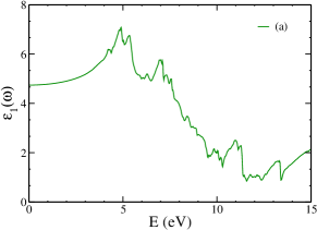
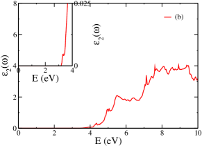
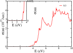
Figure 6: (Color online). (a) Calculated, dispersive part, $\varepsilon_{1}(\omega)$, of the dielectric function of c-SrTiO₃ as obtained with the optimal basis set using PW - GGA. (b) Calculated, absorptive part, $\varepsilon_{2}(\omega)$, of the dielectric function of c-SrTiO₃ as obtained with the optimal basis set using PW - GGA. (c) Calculated, optical conductivity, $\sigma(\omega)$, of c-SrTiO₃ as obtained with the optimal basis set using PW - GGA. As per the inserts (see Figs. 6(b) and  6(c)), the band absorption edge is at 3.24 eV. In all cases, spectra have been calculated without any broadening.

From our calculated DOS (see Fig. 3(a)), it can be inferred that the onset of absorption is quite sharp and it starts at about 3.24 eV. It exhibits a fine structure at 3.6 eV, with a shoulder at 4.50 eV. This picture is consistent with the experimental results of  Cohen and Blunt Cohen and Blunt (1968) and the theoretical findings of  Perkins and Winter Perkins and Winter (1983) of a relatively sharp absorption edge in the optical measurement of SrTiO₃. In the calculated DOS of the low laying conduction bands, sharp peaks appear at 4.70 eV, 5.72 eV, and 7.05 eV. Relatively broad peaks are found at 8.33 eV, 10.97 eV and 12.75 eV. Our computed peaks are in basic agreement with experimental findings of  Cardona Cardona (1965) and  Braun et al. Braun et al. (1978). For the valence bands DOS, we calculated peaks at -0.20 eV, -0.72 eV, -1.14 eV, -1.83 eV, -2.86 eV, -4.06 eV, -4.50 eV, -14.30 eV, -4.61 eV, and -17.53 eV. The peaks in the valence band DOS are all sharp. Our calculated electronic structure is in agreement with scanning transmission electron microscopy, vacuum ultraviolet spectroscopy, and spectroscopic ellipsometry measurement of  Van Benthem et al. Van Benthem et al. (2001).

Our calculated band gap value of 3.24 eV, from $L$ to $\Gamma$, is practical the same as the experimental one. In general, other theoretical calculations obtained values that are up to 1.1 eV smaller. The source of the small band gap values was believed to be due to the pushing up of the top of the valence band dominated by Ti 3d and O 2p states to higher energies Pertosa and Michel-Calendini (1978). According to our findings, it rather appears to be the extra lowering of the conduction bands that produces GGA (or LDA) band gaps that are more than 1.1 eV smaller than the experimental values, if LCAO type computations do not search for and utilize an optimal basis set. Such a basis set is verifiably converged for the description of occupied states Ekuma et al. (2011a, b); Bagayoko et al. (2004). We recall that Kohn and Sham Kohn and Sham (1965), in their original paper, explicitly stated the need to solve self consistently the pertinent system of equations defining LDA. The BZW method, as explained above, rigorously solves the system of equations in the sense explained above. Single trial basis set calculations also involve both the KS and charge density equations. The major difference resides in the fact that these calculations do not generally entail changes in the basis functions beyond those of the expansion coefficients.

III.3 Structural Properties

The total energy versus the lattice constant data are shown in Fig. 5. The data fit well to the Murnaghan equation of state (EOS). The calculated equilibrium lattice constant is 3.92 Å and the bulk modulus, $B_{o}$, is 183.45 GPa.

The experimently reported lattice constants are in the range 3.89 to 3.92 Å ICSD (2011); Wyckoff (1963); Hellwege and Hellwege (1969); Mo et al. (1999) and the bulk modulus lays in the range 174 to 183 GPa Wyckoff (1963); Hellwege and Hellwege (1969); Mo et al. (1999). In Table 3, we show our calculated equilibrium lattice constant and bulk modulus in comparison with experimental and other theoretical results. Both our calculated lattice constant and bulk modulus agree well with corresponding, experimental ones, respectively.

III.4 Optical Properties

The plot of the dispersive ($\varepsilon_{1}(\omega)$) and absorptive ($\varepsilon_{2}(\omega)$) dielectric functions are shown in Figs. 6(a) and 6(b), respectively, while the optical conductivity ($\sigma(\omega)$) profile is in Fig. 6(c). All reported spectra have been calculated without any broadening and, may have more features than experimental ones. Our calculated, dielectric spectra are in good agreement with the experimental measurementsCardona (1965); Mitsui and Nomura (1982). The calculated optical spectra only included the direct inter band transitions. The fundamental absorption edge E_o, which is also a measure of the optical gap, was found to be 3.24 eV from the calculation, as per the insert of Fig. 6(b). Our computed direct gap of 3.43 eV is in agreement with the experimental value of 3.40 eVCardona (1965); Mitsui and Nomura (1982). Our calculated $\varepsilon_{1}(\omega=0)$ at zero frequency equals 4.75 (cf. Fig. 6(a)). It compares well with the experimental value of 4.92 measured by  Braun et al. Braun et al. (1978). Our dielectric spectra resemble that of BaTiO₃ of  Bagayoko et al. Bagayoko et al. (1998). This observation also holds for the data of  Cardona Cardona (1965) and  Baurerle et al. Baurerle et al. (1978). Both the experimental and our calculated results show that the direct optical gap is larger than the smallest indirect band gap.

Figure 6(c) shows the optical conductivity $\sigma(\omega)$ of SrTiO₃. As per the insert, it also shows that the fundamental absorption edge starts at 3.24 eV. The positions of the peaks (without any rigid shift) are in agreement with experimental findings.

IV Summary and Conclusion

We have performed first principle, ab initio calculations of the electronic, structural, elastic, and optical properties of bulk SrTiO₃ in the cubic phase using GGA potential and the BZW method. Our calculated results, without any adjustment or corrections, show good agreement with experimental data.

The agreement of our calculated band gaps (3.21 and 3.24 eV) and electron effective masses with corresponding, experimental values is significant. Some calculations with adjustable parameters can lead to the correct band gap; but they generally do not yield the correct curvature of the conduction band around its minimum-as given by the electron effective masses. Similarly, the agreement between the peaks in the calculated density of states with corresponding, experimental ones denote the correct description of the relative location of the bands. This result is confirmed by our reproduction of the measured features of the dielectric functions, the imaginary part of which was obtained using only direct transitions between occupied and unoccupied bands. Our calculated equilibrium lattice constant (3.92 Å) and bulk modulus (183.45 GPa) also agree with corresponding, experimental findings.