Creating vortons and three-dimensional skyrmions from domain wall annihilation with stretched vortices in Bose-Einstein condensates

Abstract

We study a mechanism to create a vorton or three-dimensional skyrmion in phase-separated two-component BECs with the order parameters $\Psi_{1}$ and $\Psi_{2}$ of the two condensates. We consider a pair of a domain wall (brane) and an anti-domain wall (anti-brane) stretched by vortices (strings), where the $\Psi_{2}$ component with a vortex winding is sandwiched by two domains of the $\Psi_{1}$ component. The vortons appear when the domain wall pair annihilates. Experimentally, this can be realized by preparing the phase separation in the order $\Psi_{1}$, $\Psi_{2}$ and $\Psi_{1}$ components, where the nodal plane of a dark soliton in $\Psi_{1}$ component is filled with the $\Psi_{2}$ component with vorticity. By selectively removing the filling $\Psi_{2}$ component gradually with a resonant laser beam, the collision of the brane and anti-brane can be made, creating vortons.

I Introduction

Quantized vortices are one of remarkable consequences of superconductivity and superfluidity. In multi-component superfluids and superconductors, there appear many kinds of exotic vortices. When a vortex of one condensate traps another condensate inside its core, a supercurrent or superflow of the latter can exist along the vortex line. Such a vortex is called a superconducting or superflowing cosmic string in cosmology Witten:1984eb . Because of the Meissner effect, superconducting strings exclude magnetic fields like superconductive wires, so that they are proposed to explain several cosmological phenomena related to galactic magnetic fields. When a superconducting string is closed and “twisted”, i.e., when the second condensate inside the string core has a non-trivial winding along the string loop, the supercurrent persistently flows along the loop and makes it stable. Such a twisted vortex loop is called a “vorton”, a particle-like soliton made of a vortex Davis:1988jq ; Radu:2008pp . While vortons were discussed in ³He superfluids Volovik , they are considered to be a candidate of dark matter, and a possible source of ultra high energy cosmic ray. There have been a lot of study about their stability, interaction, and applications to cosmology Vilenkin:2000 .

On the other hand, three-dimensional (3D) skyrmions are topological solitons (textures) characterized by the third homotopy group $\pi_{3}(SU(2))\simeq{\bf Z}$ in a pion effective field theory. Skyrmions were proposed to be baryons Skyrme:1961vq . Since their proposal, the skyrmions have been studied for a long time about their stability, interaction, and applications to nuclear physics Manton:2004tk .

Both 3D skyrmions and vortons have been fascinating subjects in high energy physics and cosmology for decades, and a lot of works have been done already, but they have yet to be observed in nature. On the other hand, these topological excitations, 3D skyrmions Ruostekoski:2001fc ; Battye:2001ec ; 3D-Skyrmions2 ; Savage:2003hh ; Ruostekoski:2004pj ; Wuster:2005 ; Oshikawa:2006 and vortons Metlitski:2003gj ; Bedaque:2011sb , can be realized in Bose–Einstein condensates (BECs) of ultracold atomic gasses. Moreover 3D skyrmions and vortons have been shown to be topologically equivalent in two-component BECs Ruostekoski:2001fc ; Battye:2001ec . BECs are extremely flexible systems for studying solitons (or topological defects) since optical techniques can be used to control and directly visualize the condensate wave functions Leslie:2009 . Interest in various topological defects in BECs with multicomponent order parameters has been increasing; the structure, stability, and creation and detection schemes for monopoles Stoof ; Martikainen ; Savage ; Pietila:2009 , knots Kawaguchi:2008xi and non-Abelian vortices Semenoff:2006vv have been discussed review .

It is, however, still unsuccessful to create vortons and 3D skyrmions experimentally, although the schemes to create and stabilize them have been theoretically proposed Ruostekoski:2001fc ; Battye:2001ec ; 3D-Skyrmions2 ; Savage:2003hh ; Ruostekoski:2004pj ; Wuster:2005 ; Oshikawa:2006 . In the present study, we propose how to create vortons or 3D skyrmions in two-component BECs from domain walls and quantized vortices. Specific examples of the system include a BEC mixture of two-species atoms such as ⁸⁷Rb–⁴¹K Thalhammer or ⁸⁵Rb–⁸⁷Rb Papp , where the miscibility and immiscibility can be controlled by tuning the atom–atom interaction via Feshbach resonances. Here, the domain wall is referred to as an interface boundary of phase-separated two-component BECs. Although the interface has a finite thickness, the wall is well-defined as the plane in which both components have the same amplitude. Since a description of two-component BECs can be mapped to the $O(3)$ nonlinear sigma model (NL$\sigma$M) by introducing a pseudospin representation of the order parameter Kasamatsu2 ; Babaev:2001zy ; Babaev:2008zd , the resultant wall–vortex composite soliton corresponds to the Dirichlet(D)-brane soliton described in Refs. Gauntlett:2000de ; Shifman:2002jm ; Isozumi:2004vg ; Eto:2006pg ; Eto:2008mf , which resembles a D-brane in string theory Polchinski:1995mt ; Leigh ; Polchinskibook . Such a D-brane soliton has been already numerically constructed by us in two-component BECs Kasamatsu:2010aq . We have found that these composite solitons are energetically stable in rotating, trapped BECs and are experimentally feasible with realistic parameters. Similar configuration has been also studied in spinor BECs Borgh:2012es .

A brane–antibrane annihilation was demonstrated to create some topological defects in superfluid ³He Bradley . However, a physical explanation of the creation mechanism of defects still remains unclear. The intriguing experiment that mimicked the brane–antibrane annihilation was performed in cold atom systems with the order parameters $\Psi_{1}$ and $\Psi_{2}$ of two-component BECs by Anderson et al. Anderson . They prepared the configuration of the phase separation in the order $\Psi_{1}$, $\Psi_{2}$ and $\Psi_{1}$ components, where the nodal plane of a dark soliton in one component was filled with the other component. By selectively removing the filling component with a resonant laser beam, they made a planer dark-soliton in a single-component BEC. Then, the planer dark soliton in 3D system is dynamically unstable for its transverse deformation (known as snake instability) Anderson , which results in the decay of the dark soliton into vortex rings. In the two-component BECs, we have numerically simulated brane–anti-brane annihilations, which resulted in vortex loops Takeuchi:2011 .

In this paper, we consider a junction of a D-brane soliton and its anti-soliton, namely a pair of a domain wall and an anti-domain wall stretched by vortices. We give an approximate analytic solution for a pair of the D-brane and anti-D-brane in the $O(3)$ NL$\sigma$M. We show that this unstable configuration decays into a vorton or a 3D skyrmion, instead of an untwisted vortex ring Anderson in the case without stretched vortices. Experimentally, this can be realized by preparing the phase separation in the order $\Psi_{1}$, $\Psi_{2}$ and $\Psi_{1}$ components, and rotating the intermediate $\Psi_{2}$ component. By selectively removing the filling $\Psi_{2}$ component gradually with a resonant laser beam, the collision of the D-brane and anti-D-brane can be made, to create vortons.

This paper is organized as follows. In Sec. II, we present the Gross-Pitaevski energy functional of two-component BECs, and rewrite it in the form of NL$\sigma$M. In Sec. III, after constructing a phase separation, i.e., a domain wall configuration in NL$\sigma$M, we consider a pair of a domain wall and an anti-domain wall. We discuss a creation of vortex in two dimensions, and a creation of vortex loops in three dimensions after a pair annihilation of the domain walls. In Sec. IV, we consider a pair of a domain wall and an anti-domain wall with vortices stretched between them. We show that when a vortex loop encloses $n$ of the stretched vortices, the phase of the $\Psi_{2}$ component winds $n$ times, i.e., it is a vorton with $n$ twist. We also confirm a vorton with $n=1$ is topologically equivalent to a 3D skyrmion. Sec. V is devoted to a summary and discussion.

II System

II.1 Gross-Pitaevski energy functional

The order parameter of two-component BECs is

$${\bf\Psi}=(\Psi_{1},\Psi_{2}),$$ (1)

where

$$\Psi_{j}=\sqrt{\rho_{j}}e^{i\theta_{j}}\quad(j=1,2)$$ (2)

are the macroscopically occupied spatial wave function of the two components with the density $\rho_{j}$ and the phase $\theta_{j}$. The order parameter can be represented by the pseudospin

$${\bf s}=(s_{1},s_{2},s_{3})=(\sin\theta\cos\phi,\sin\theta\sin\phi,\cos\theta)$$ (3)

with a polar angle $\theta=\cos^{-1}[(\rho_{1}-\rho_{2})/\rho]$ and an azimuthal angle $\phi=\theta_{2}-\theta_{1}$ as

$${\bf\Psi}=\sqrt{\rho}e^{i\frac{\Theta}{2}}\left(\cos\frac{\theta}{2}e^{-i\frac{\phi}{2}},\sin\frac{\theta}{2}e^{i\frac{\phi}{2}}\right),$$ (4)

where $\rho=\rho_{1}+\rho_{2}$ and $\Theta=\theta_{1}+\theta_{2}$ represent the local density and phase, respectively Kasamatsu2 .

The solutions of the solitonic structure in two-component BECs are given by the extreme of the Gross–Pitaevski (GP) energy functional

$$E[{\bf\Psi}]=\int d^{3}x\biggl{\{}\sum_{j=1,2}\biggl{[}\frac{\hbar^{2}}{2m_{j}}\left|\nabla\Psi_{j}\right|^{2}+(V_{j}-\mu_{j})|\Psi_{j}|^{2}$$

$$+\frac{g_{jj}}{2}|\Psi_{j}|^{4}\biggr{]}+g_{12}|\Psi_{1}|^{2}|\Psi_{2}|^{2}\biggr{\}}.$$ (5)

Here, $m_{j}$ is the mass of the $j$th component and $\mu_{j}$ is its chemical potential. The BECs are confined by the harmonic trap potential

$$V_{j}=\frac{1}{2}m_{j}(\omega_{x}^{2}x^{2}+\omega_{y}^{2}y^{2}+\omega_{z}^{2}z^{2}).$$ (6)

The coefficients $g_{11}$, $g_{22}$, and $g_{12}$ represent the atom–atom interactions. They are expressed in terms of the s-wave scattering lengths $a_{11}$ and $a_{22}$ between atoms in the same component and $a_{12}$ between atoms in the different components as

$$g_{jk}=\frac{2\pi\hbar^{2}a_{jk}}{m_{jk}}$$ (7)

with $m_{jk}^{-1}=m_{j}^{-1}+m_{k}^{-1}$. The GP model is given by the mean-field approximation for the many-body wave function and provides quantitatively good description of the static and dynamic properties of the dilute-gas BECs Pethickbook .

II.2 Mapping to the nonlinear sigma model

To derive the generalized NL$\sigma$M for two-component BECs from the GP energy functional (5), we assume $m_{1}=m_{2}=m$ and $V_{1}=V_{2}=V$. By substituting the pseudospin representation Eq.(4) of ${\bf\Psi}$, we obtain Kasamatsu2

$$E=\int d^{3}x\biggl{\{}\frac{\hbar^{2}}{2m}\biggl{[}(\nabla\sqrt{\rho})^{2}+\frac{\rho}{4}\sum_{\alpha=1}^{3}(\nabla s_{\alpha})^{2}\biggr{]}+V\rho$$

$$+\frac{m\rho}{2}|{\bf v}_{\rm eff}|^{2}+c_{0}+c_{1}s_{3}+c_{2}s_{3}^{2}\biggr{\}},$$ (8)

where we have introduced the effective superflow velocity

$${\bf v}_{\rm eff}=\frac{\hbar}{2m}(\nabla\Theta-\cos\theta\nabla\phi)$$ (9)

and the coefficients

$$c_{0} = \frac{\rho}{8}[\rho(g_{11}+g_{22}+2g_{12})-4(\mu_{1}+\mu_{2})],$$ (10)

$$c_{1} = \frac{\rho}{4}[\rho(g_{11}-g_{22})-2(\mu_{1}-\mu_{2})],$$ (11)

$$c_{2} = \frac{\rho^{2}}{8}(g_{11}+g_{22}-2g_{12}).$$ (12)

The coefficient $c_{1}$ can be interpreted as a longitudinal magnetic field that aligns the spin along the $x^{3}$-axis; it was assumed to be zero in this study. The term with the coefficient $c_{2}$ determines the spin–spin interaction associated with $s_{3}$; it is antiferromagnetic for $c_{2}>0$ and ferromagnetic for $c_{2}<0$ Kasamatsu2 . Phase separation occurs for $c_{2}<0$, which we are focusing on. Further simplification can be achieved by assuming that $V=0$ and the total density is uniform through the relation $\rho=\mu/g$ where $g=g_{11}=g_{22}$ and $\mu=\mu_{1}=\mu_{2}$, and that the kinetic energy associated with the superflow ${\bf v}_{\rm eff}$ is negligible. Although the assumptions ${\bf v}_{\rm eff}=0$ and $\rho$=const. become worse in the vicinities of vortex cores or domain walls, this simplification does not affect on later discussions about the vorton nucleations based on topology.

By using the healing length $\xi=\hbar/\sqrt{2mg\rho}$ as the length scale, the total energy can reduce to

$$\tilde{E}=\frac{E}{g\rho\xi^{3}}=\int d^{3}x\frac{1}{4}\left[\sum_{\alpha=1}^{3}(\nabla s_{\alpha})^{2}+M^{2}(1-s_{3}^{2})\right],\quad\quad$$ (13)

$$M^{2}=\frac{4|c_{2}|}{g\rho^{2}},$$ (14)

where $M$ is the effective mass for $s_{3}$. This is a well-known massive NL$\sigma$M for effective description of a Heisenberg ferromagnet with spin–orbit coupling.

Introducing a stereographic coordinate

$$u={s_{1}-is_{2}\over 1-s_{3}},$$ (15)

we can rewrite Eq. (13) as

$$\tilde{E}=\int d^{3}x\frac{\sum_{\alpha=1}^{3}|\partial_{\alpha}u|^{2}+M^{2}|u|^{2}}{(1+|u|^{2})^{2}}.$$ (16)

Here, $u=0$ $(\infty)$ corresponds to the south (north) pole of the $S^{2}$ target space.

III Wall – anti-wall annihilation

III.1 Domain walls

For a domain wall perpendicular to the $x^{1}$-axis, $u=u(x^{1})$, the total energy is bounded from below by the Bogomol’nyi–Prasad–Sommerfield (BPS) bound as Gauntlett:2000de ; Isozumi:2004vg ; Eto:2006pg ; Kasamatsu:2010aq

$$\tilde{E} = \int d^{3}x\frac{|\partial_{1}u\mp Mu|^{2}\pm M(u^{\ast}\partial_{1}u+u\partial_{1}u^{\ast})}{(1+|u|^{2})^{2}}$$ (17)

$$\geq |T_{\rm w}|$$

by the topological charge that characterizes the wall:

$$T_{\rm w}=M\int d^{3}x\frac{u^{\ast}\partial_{1}u+u\partial_{1}u^{\ast}}{(1+|u|^{2})^{2}},$$ (18)

where $\partial_{i}$ denotes the differentiation with respect to $x^{i}$. Among all configurations with a fixed boundary condition, i.e., with a fixed topological charge $T_{\rm w}$, the most stable configurations with the least energy saturate the inequality (17) and satisfy the BPS equation

$$\partial_{1}u\mp Mu=0,$$ (19)

which is obtained by $|...|^{2}=0$ in Eq. (17). This equation immediately gives the analytic form of the wall configuration

$$u_{\rm w}(x^{1})=e^{\mp M(x^{1}-x^{1}_{0})-i\phi_{0}}.\hskip 8.53581pt$$ (20)

The function $u_{\rm w}$ represents the domain wall with wall position $x^{1}_{0}$ and phase $\phi_{0}$ associated with $(s_{1},s_{2})$; this phase $\phi_{0}$ yields the Nambu–Goldstone mode localized on the wall, as in Fig. 1. The sign $\mp$ implies a domain wall and an anti-domain wall. The domain wall can be mapped to a path in the target space as shown in Fig. 2(a).

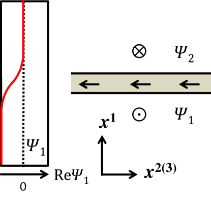
(a)                 (b)

Figure 1: (Color online) A single domain wall in two-component BECs. (a) The amplitude of $\Psi_{1}$ for a domain wall. (b) The pseudospin texture of the single domain wall perpendicular to the $x^{1}$-axis in real space. The arrows denote points in the target space $S^{2}$. The gradient and interaction energies are localized around the wall, which is shaded schematically. The arrows on the wall imply the phase $\phi_{0}$ which the wall possesses.

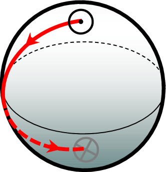
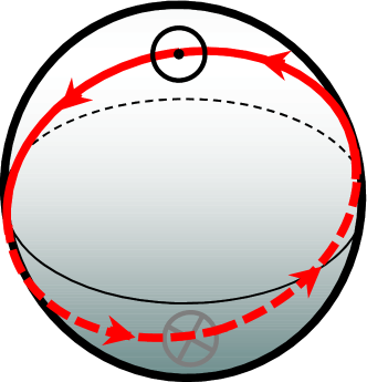
(a)                                   (b)

Figure 2: (Color online) The $S^{2}$ target space where the north and south poles are denoted by $\odot$ and $\otimes$, respectively.
(a) The path connecting the north and south poles represents the map from the path in the domain wall in Fig. 1(b) along the $x^{1}$-axis in real space from $x^{1}\to-\infty$ to $x^{1}\to+\infty$. The path in the $S^{2}$ target space passes through one point on the equator, which is represented by “$\leftarrow$” in Fig. 1(b) in this example. In general, the $U(1)$ zero mode is localized on the wall.
(b) The path in the target space $S^{2}$ for a domain wall and an anti-domain wall. The path represents the map from the path along the $x^{1}$-axis from $x^{1}\to-\infty$ to $x^{1}\to+\infty$ in real space in Fig. 3(b).

III.2 Wall anti-wall annihilation

As described in Sec.I, we note that the intriguing experiment that mimicked the brane–antibrane annihilation was performed by Anderson et al. Anderson . They created the configuration shown in Fig. 3, where the nodal plane of a dark soliton in one component was filled with the other component. By selectively removing the filling component with a resonant laser beam, they made a planer dark-soliton in a single-component BEC. The dark soliton corresponds to the coincident limit of the two kinks in Fig. 3(a). It is known that the planer dark soliton in the 3D system is dynamically unstable for its transverse deformation (known as snake instability) Anderson , which results in the decay of the dark soliton into vortex rings.

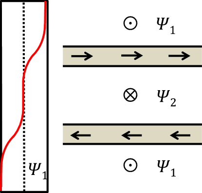
(a)                 (b)

Figure 3: (Color online) A pair of domain wall and anti-domain wall in two-component BECs. (a) The amplitude of $\Psi_{1}$ for the wall and anti-wall configuration. (b) The pseudo-spin texture of the wall and anti-wall configuration in real space. The arrows denote the pseudo-spin. $\Psi_{1}$ ($\Psi_{2}$) is filled outside (between) the walls, where the other component is zero. In the upper (lower) region outside the walls, the phase of $\Psi_{1}$ is fixed to be zero ($\pi$).

In our context, this experiment demonstrated the wall–anti-wall collision and subsequent creation of cosmic strings, where the snake instability may correspond to “tachyon condensation” in string theory Sen . The procedure that removes the filling component can decrease the distance $R$ between two domain walls and cause their collision. The tachyon condensation can leave lower dimensional topological defects after the annihilation of D-brane and anti-D-brane. In our case of the phase-separated two-component BECs, the annihilation of the 2-dimensional defects (domain walls) leaves 1-dimensional defects (quantized vortices).

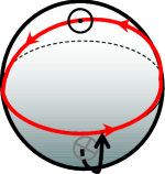
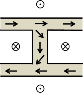
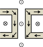
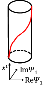
(a)                               (c)                               (e)                        (g)

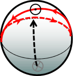
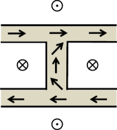
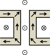
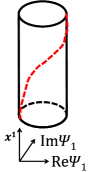
(b)                               (d)                               (f)                        (h)

Figure 4: (Color online) Decaying processes of the wall-anti-wall pair. (a,b) The loop in the pseudo-spin space is unwound in two ways. (c,d) A bridge is created between the wall and anti-wall. In this process there are two possibilities of spin structure along the bridge. (e,f) The upper and lower regions are connected with a ‘passage’ through the bridge being formed. (g,h) The $\Psi_{1}$ component is filled inside the passage, and the phase of $\Psi_{1}$ component is connected anti-clockwise or clockwise.

Let us discuss this in two dimensions in more detail. Here $U(1)$ zero modes of the wall and the anti-wall are taken to be opposite as in Fig. 3 (b). The configuration is mapped to a loop in the $S^{2}$ target space, see Fig. 2 (b). This configuration is unstable. It should end up with the vacuum with the up-spin $\odot$. In the decaying process the loop is unwound from the south pole in the target space. To do this there are two topologically inequivalent ways, which are schematically shown in (a) and (b) in Fig. 4. In real space, at first, a bridge connecting two walls is created as in (c) and (d) in Fig. 4. Here, there exist two possibilities of the spin structure of the bridge, corresponding to two ways of the unwinding processes. Along the bridge in the $x^{1}$-direction, the spin rotates (c) anti-clockwise or (d) clockwise on the equator of the $S^{2}$ target space. Let us label these two kinds of bridges by “$\downarrow$” and “$\uparrow$”, respectively.

In the next step, a ‘passage’ through the bridge is formed as in (e) and (f) in Fig. 4, where the ground state, i.e., the up-spin $\odot$ state, is filled between them. The phase of the filling $\Psi_{1}$ component through the passage is connected anti-clockwise or clockwise [Fig. 4 (g) and (h)] Let us again label these two kinds of passages by “$\downarrow$” and “$\uparrow$”, respectively. In either case, the two regions separated by the domain walls are connected through a passage created in the decay of domain walls. Once created, these passages grow to holes in order to reduce the domain wall energy.

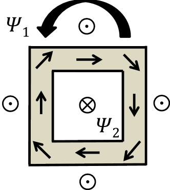
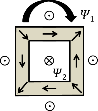
(a)                           (b)

(c)                           (d)

Figure 5: (Color online) Stable and unstable wall rings. (a,b) Stable wall rings. The domain wall phase winds once (the winding number is $\pm 1$) along the rings. Total configurations are 2d skyrmions with a non-trivial element $\pm 1$ of the second homotopy group $\pi_{2}$. The phase $\Psi_{1}$ winds $\pm 1$ so that it is a vortex, while $\Psi_{2}$ is filled inside the core. (c,d) Unstable wall rings. The domain wall phase does not wind (the winding number is $0$) along the rings. The phase $\Psi_{1}$ does not wind so that it cannot be a vortex, while $\Psi_{2}$ is filled inside the ring. They decay into ground state (up pseudo-spin).

Several holes are created in the entire decaying process. Let us focus a pair of two neighboring holes. Then, one can find a ring of a domain wall between the holes as shown in Fig. 5. Here, since there exist two kinds of holes ($\uparrow$ and $\downarrow$), there exist four possibilities of the rings, (a) $\uparrow\downarrow$, (b) $\downarrow\uparrow$, (c) $\uparrow\uparrow$ and (d) $\downarrow\downarrow$ in Fig. 5. In all the cases, the $\Psi_{2}$ component is confined in the domain wall rings. The phase of $\Psi_{1}$ component has a nontrivial winding outside the rings of types (a) and (b), whereas it does not have a winding outiside the domain wall rings of types (c) and (d). Consequently, the domain wall rings of types (c) and (d) can decay and end up with the ground state $\odot$. However, the decay of the rings of types (a) and (b) is topologically forbidden; they are nothing but coreless vortices.

In the $O(3)$ NL$\sigma$M, the domain wall rings of types (a) of (b) are the Anderson–Toulouse vortices AndersonToulouse , or lumps in field theory Polyakov:1975yp . The solutions can be written as ($z\equiv x^{1}+ix^{2}$)

$$u=u_{0}=\sum_{i=1}^{k}{\lambda_{i}\over z-z_{i}}\quad\mbox{or}\quad u=\bar{u}_{0}$$ (21)

for a lump or an anti-lump, where $z_{i}\in{\bf C}$ represent the position of the lump while and $\lambda_{i}\in{\bf C}^{*}$ with $|\lambda_{i}|$ and $\arg\lambda_{i}$ representing the size and the $U(1)$ orientation of the lump, respectively. In fact, one can show that these configurations have a nontrivial winding in the second homotopy group $\pi_{2}(S^{2})\simeq{\bf Z}$ which can be calculated from

$${1\over 2\pi}\int d^{2}x\,{i(\partial_{1}u^{*}\partial_{2}u-\partial_{2}u^{*}\partial_{1}u)\over(1+|u|^{2})^{2}}.$$ (22)

The wall rings of (a) and (b) in Fig. 5 belong to $+1$ and $-1$ of $\pi_{2}(S^{2})$, respectively. Namely they are a lump and an anti-lump, respectively.

So far we have discussed two dimensional space in which domain wall is a line and a vortex is point-like. In three dimensions, domain walls have two spatial dimensions. When the decay of the domain wall pair occurs, there appear two-dimensional holes, which can be labeled by $\downarrow$ or $\uparrow$ in Fig. 6(a). Along the boundary of these two kinds of holes, there appear vortex lines, which in general making vortex loops, as in Fig. 6(b). This process has been numerically demonstrated Takeuchi:2011 . The vortex rings decay into the fundamental excitations in the end.

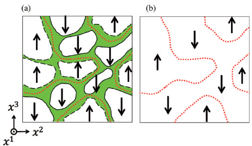
Figure 6: (Color online) Decay of a domain wall pair in three dimensions. Domain walls are two-dimensional objects. (a) Two kinds of holes labeled by $\uparrow$ and $\downarrow$ are created after a domain-wall pair decay. (b) Along the boundary of these two kinds of holes, there appear vortex lines (denoted by dotted lines), which in general making vortex loops.

IV D-brane – anti-D-brane annihilation

IV.1 D-brane soliton

The D-brane soliton by Gauntlett et. al. Gauntlett:2000de can be reproduced in two-component BECs as follows Kasamatsu:2010aq . For a fixed topological sector, vortices (a domain wall) parallel (perpendicular) to the $x^{1}$-axis, the total energy is bounded from below by the BPS bound as Gauntlett:2000de ; Isozumi:2004vg ; Eto:2006pg ; Kasamatsu:2010aq

$$\tilde{E} = \int d^{3}x\frac{|\partial_{1}u\mp Mu|^{2}+|(\partial_{2}\mp i\partial_{3})u|^{2}}{(1+|u|^{2})^{2}}$$ (23)

$$\pm \int d^{3}x\frac{M(u^{\ast}\partial_{1}u+u\partial_{1}u^{\ast})+i(\partial_{2}u^{\ast}\partial_{3}u-\partial_{3}u^{\ast}\partial_{2}u)}{(1+|u|^{2})^{2}}$$

$$\geq |T_{\rm w}|+|T_{\rm v}|$$

by the topological charges that characterize the wall and vortices:

$$T_{\rm w} = M\int d^{3}x\frac{u^{\ast}\partial_{1}u+u\partial_{1}u^{\ast}}{(1+|u|^{2})^{2}},$$ (24)

$$T_{\rm v} = i\int d^{3}x\frac{\partial_{2}u^{\ast}\partial_{3}u-\partial_{3}u^{\ast}\partial_{2}u}{(1+|u|^{2})^{2}}.$$ (25)

Then, the least energy configurations with fixed topological charges (a wall with a fixed number of vortices) satisfy the BPS equations

$$\partial_{1}u\mp Mu=0,\hskip 17.07164pt(\partial_{2}\mp i\partial_{3})u=0.$$ (26)

The analytic form of the wall–vortex composite solitons can be found ($z\equiv x^{2}+ix^{3}$)

$$u(x^{1},z)=u_{\rm w}(x^{1})u_{\rm v}(z),$$ (27)

where Isozumi:2004vg

$$u_{\rm w}(x^{1})=e^{\mp M(x^{1}-x^{1}_{0})-i\phi_{0}},$$ (28)

$$\hskip 8.53581ptu_{\rm v}(z)=\frac{\prod_{j=1}^{N_{v_{1}}}(z-z_{j}^{(1)})}{\prod_{j=1}^{N_{v_{2}}}(z-z_{j}^{(2)})}.$$ (29)

The function $u_{\rm w}$ represents the domain wall with wall position $x^{1}_{0}$ and phase $\phi_{0}$. The function $u_{\rm v}$ gives the vortex configuration, being written by arbitrary analytic functions of $z$; the numerator represents $N_{v_{1}}$ vortices in one domain ($\Psi_{1}$ component) and the denominator represents $N_{v_{2}}$ vortices in the other domain ($\Psi_{2}$ component). The positions of the vortices are denoted by $z_{j}^{(1)}$ and $z_{j}^{(2)}$. The total energy does not depend on the form of the solution, but only on the topological charges as $T_{\rm w}=\pm M$ or 0 (per unit area), and $T_{\rm v}=2\pi N_{\rm v}$ (per unit length), where $N_{\rm v}$ is the number of vortices passing through a certain $x^{1}=$ const plane.

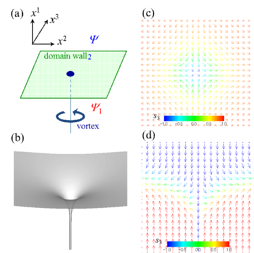
Figure 7: (Color online) The typical D-brane soliton in two-component BECs. (a) Schematic illustration of the wall-vortex soliton configuration viewed from the length scale larger than the domain-wall width and the vortex core size. The two-component BECs $\Psi_{1}$ ($x^{1}<0$) and $\Psi_{2}$ ($x^{1}>0$) are separated by the domain wall. A single vortex located at $x^{1}<0$ ($\Psi_{1}$ component) is connected to the domain wall. (b) The isosurface of $s_{3}=0$ for the solution Eq. (27) of the NL$\sigma$M, where $M=1$, $x_{0}^{1}=0$, $\phi_{0}=0$, $N_{v1}=1$, $N_{v2}=0$, and $z_{1}^{(1)}=0$. The corresponding spin textures ${\bf s}$ in the $z=0$ plane and $y=0$ plane are shown in (c) and (d), respectively. The magnitude of $s_{3}$ is denoted by color. We have ${\bf s}=(0,0,-1)$ along the vortex core.

Figure 7 shows a D-brane soliton with the simplest wall–vortex configuration of Eq. (27). A vortex exists in $x^{1}<0$ and forms a texture, where the spin points down at the center and rotates continuously from down to up as it moves radially outward. The edge of vortex attaches to the wall, causing it to bend logarithmically as $x^{1}=\log|z|/M$ [Fig. 7(b) and (d)]. We can construct solutions in which an arbitrary number of vortices are connected to the domain wall by multiplying by the additional factors $z-z_{j}^{(i)}$ [see Eq. (29)]; Fig. 8 shows a solution in which both components have one vortex connected to the wall. In the NL$\sigma$M, the energy is independent of the vortex positions $z_{j}^{(i)}$ on the domain wall; in other words, there is no static interaction between vortices.

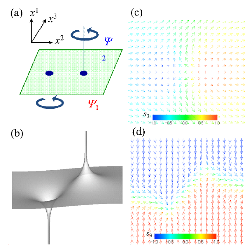
Figure 8: (Color online) The D-brane soliton to which two vortices attach. (a) Schematic illustration of the configuration in which each component has a single vortex connected to the wall. (b) The isosurface of $s_{3}=0$ for the solution Eq. (27) of the NL$\sigma$M, where $M=1$, $x_{0}^{1}=0$, $\phi_{0}=0$, $N_{v1}=1$, $N_{v2}=1$, $z_{1}^{(1)}=-2$, and $z_{1}^{(2)}=2$. The corresponding spin textures ${\bf s}$ in the $z=0$ plane and $y=0$ plane are shown in (c) and (d), respectively. The magnitude of $s_{3}$ is denoted by color. The wall becomes asymptotically flat due to the balance between the tensions of the attached vortices.

IV.2 Brane-anti-brane annihilation with a string

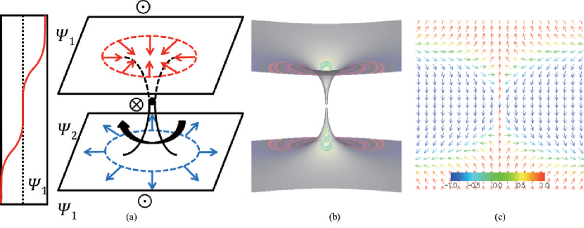
Figure 9: (Color online) (a) A pair of a D-brane (domain wall) and an anti-D-brane (anti-domain wall) stretched by a string (vortex) in two-component BECs. The branes are perpendicular to the $x^{1}$-axis and the string is placed along the $x^{1}$-axis. The arrows denote pseudo-spins. The $\Psi_{1}$ ($\Psi_{2}$) component is filled outside (between) the branes, where the other component is zero. In the upper (lower) region outside the branes, the phase of $\Psi_{1}$ is fixed to be zero ($\pi$). In the middle region, the phase of $\Psi_{2}$ has winding around the vortex placed at the $x^{1}$-axis. Accordingly, the pseudo-spin rotates once (anti-)clockwise at the endpoint of string on the (anti-)brane. The profile of the $\Psi_{1}$ component along a line parallel to the $x^{1}$-axis at $(x^{2},x^{3})\neq 0$ represents two kinks in the left pannel, while the profile of the $\Psi_{1}$ component along the $x^{1}$-axis shows the coincident two kinks, i.e., a dark soliton. The dot in the center denotes the point $(\Psi_{1},\Psi_{2})=0$, which corresponds to a singularity in the NL$\sigma$M approximation ($\rho$ = const.) in (b). (b) The isosurface of $s_{3}=0$ of an approximate solution in Eq. (30) with a domain wall and an anti-domain wall stretched by a vortex in the $O(3)$ NL$\sigma$M, where $M=1$, $x_{1}^{1}=-3$, $x_{2}^{1}=3$, $\phi_{1}=0$, $\phi_{2}=\pi$. (c) The pseudo-spin texture of an approximate solution in Eq. (30).

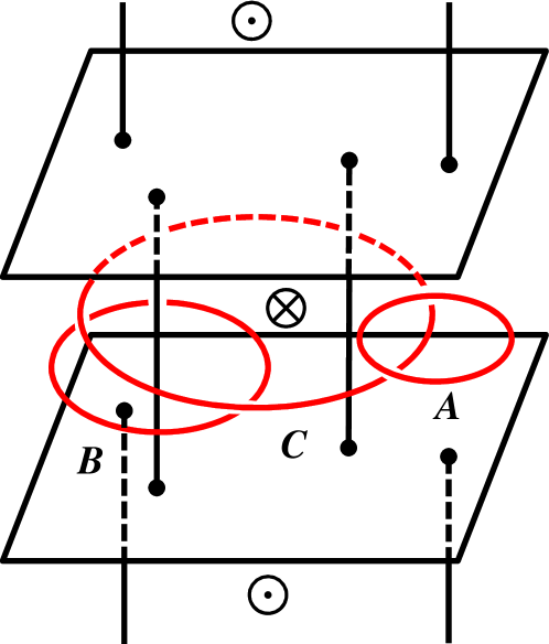
Figure 10: (Color online) Loops in the wall-vortex systems. While the loop A yields an untwisted vortex ring in Fig. 11(a), the loop B (C) yields a vorton, i.e., a vortex ring twisted once (twice). A vorton with twisted once is shown in Fig. 11(b).

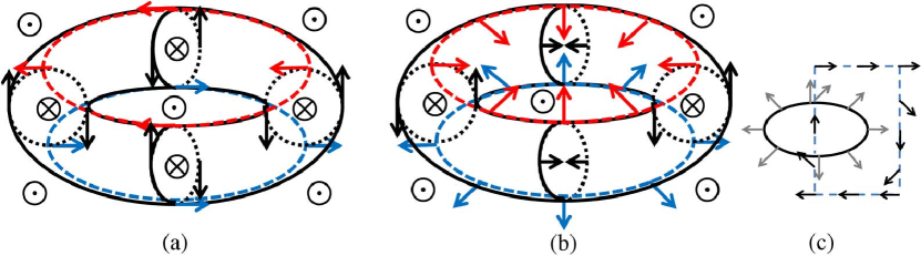
Figure 11: (Color online) (a) The pseudo-spin texture of an untwisted vortex-ring, and (b,c) the pseudo-spin and phase textures of a twisted vortex ring, i.e., a vorton, after the brane-anti-brane annihilation. (b) The pseudo-spin structure of the vorton. The torus divides the regions of $\Psi_{1}$ and $\Psi_{2}$ which repel each other: $\Psi_{1}$ ($\Psi_{2}$) are filled outside (inside) the torus. The vertical section of the torus by the $x^{1}$-$x^{2}$ plane is a pair of 2D skyrmions and anti-skyrmions. While they rotate along the $x^{1}$-axis their pseudo-spins are twisted. This spin texture is equivalent to that of a knot Kawaguchi:2008xi ; Babaev:2001zy ; Babaev:2008zd . (c) The phase structure of the vorton. The arrows denote the phase of $\Psi_{1}$ and $\Psi_{2}$. The circle denotes the core of vorton where $\Psi_{2}$ is filled and $\Psi_{1}$ is zero. The phase of $\Psi_{2}$ winds once along that circle. The square of the dotted line denotes a loop where $\Psi_{2}$ is zero. The phase of $\Psi_{1}$ winds once along that loop. Note that the loops of $\Psi_{1}$ and $\Psi_{2}$ are zero respectively make a link. Along the zeros of $\Psi_{1}$ ($\Psi_{2}$), the phase of $\Psi_{2}$ ($\Psi_{1}$) winds once.

We are ready to study a pair of a domain wall and an anti-domain wall stretched by vortices. An approximate analytic solution of the domain wall pair stretched by one vortex, which is schematically shown in Fig. 9(a), can be given in the $O(3)$ NL$\sigma$M as

$$u(x^{1},z)=u_{\rm w}(x^{1})u_{\rm v}(z),$$ (30)

$$u_{\rm w}(x^{1})=e^{-M(x^{1}-x^{1}_{1})-i\phi_{1}}+e^{M(x^{1}-x^{1}_{2})-i\phi_{2}},\quad$$ (31)

$$u_{\rm v}(z)={1/z}.$$ (32)

Here, $x^{1}_{1}$ and $x^{1}_{2}$ ($x_{1}^{1}<x_{2}^{1}$) represent the positions of the wall and anti-wall, respectively, while $\phi_{1}$ and $\phi_{2}$ denote the phase of the wall and anti-wall, respectively. This solution is good when the distance $|x^{1}_{1}-x^{2}_{2}|$ between the walls is large compared with the mass scale $M^{-1}$. For our purpose, the phases are taken as $\phi_{1}=\phi_{2}+\pi$, which means that the $\Psi_{1}$ component has a dark soliton when the intermediate $\Psi_{2}$ component vanishes. The isosurface of $s_{3}=0$ and the pseudospin structure of this configuration are plotted in Fig. 9(b) and (c), respectively. In order to avoid the logarithmic bending of the walls, one can use $u_{\rm v}(z)$ in Eq. (29) with $N_{v_{1}}=N_{v_{2}}$ instead of Eq. (32), as in Fig. 10. The solution in Eqs. (30)–(32) of the $O(3)$ NL$\sigma$M has a singularity at the midpoint of the vortex stretching the domain walls, as in Fig. 9. It is, however, merely an artifact in the NL$\sigma$M approximation of $\rho$ = const.; the singularity does not exist in the original theory without such the approximation, because $\rho$ varies and merely vanishes at that point.

Now let us discuss the dynamics of the wall–anti-wall configuration. As in the case without a stretched string, the configuration itself is unstable to decay, and vortex-loops are created in the $\Psi_{1}$ component. Since the $\Psi_{2}$ component is localized along the vortex core, the $s_{3}=0$ surface forms a torus (ring), where the region of $s_{3}>0$ is outside the torus whereas the region $s_{3}<0$ is inside it. As the phase of $\Psi_{2}$ component inside the ring is concerned, the vortex loops are classified into 1) the untwisted case [see Fig. 11(a)] and 2) the twisted case [see Fig. 11(b)].

1) If the closed vortex-loop encloses no stretched vortices as the loop A in Fig. 10, the vortex-loop is not twisted, as in Fig. 11(a). Equivalently, the phase of the $\Psi_{2}$ component inside the ring is not wound.

2) However, if the vortex-loop encloses $n$ stretched vortices as the loops B and C in Fig. 10, the vortex-loop is twisted $n$ times. It implies that the phase of the $\Psi_{2}$ component inside the ring is wound $n$ times. A vortex-loop twisted once, which is nothing but a vorton with the minimum twist, is shown in Fig. 11(b). The vertical section of the torus by the $x^{1}$-$x^{2}$ plane is a pair of a skyrmion (coreless vortex) and an anti-skyrmion (coreless vortex). Moreover, the presence of the stretched vortex implies that the phase winds anti-clockwise along the loops, as can be seen by the arrows on the top and the bottom of the torus in Fig. 11(b). When the 2D skyrmion pair rotate along the $x^{1}$-axis their phases are twisted and connected to each other at the $\pi$ rotation. Note that the zeros of $\Psi_{1}$ and $\Psi_{2}$ make a link. Along the zeros of $\Psi_{1}$ ($\Psi_{2}$), the phase of $\Psi_{2}$ ($\Psi_{1}$) winds once. The configuration is nothing but a vorton.

It may be interesting to point out that this spin texture is equivalent to the one of a knot soliton Kawaguchi:2008xi ; Babaev:2001zy ; Babaev:2008zd , i.e. a topologically nontrivial texture with a Hopf charge $\pi_{3}(S^{2})\simeq{\bf Z}$ in an $O(3)$ NL$\sigma$M. Mathematically, this fact implies that a vorton is Hopf fibered over a knot.

Finally, to confirm a vorton creation of a domain wall pair annihilations, we show a numerical simulation of the time-dependent GP equation $i\hbar\partial_{t}\Psi_{j}=\delta E/\delta\Psi_{j}^{\ast}$ for the domain wall pair with a stretched vortex in Fig. 12. The numerical scheme to solve the GP equation is a Crank–Nicholson method with the Neumann boundary condition in a cubic box without external potentials. The box size is $52.1\xi\times 52.1\xi\times 52.1\xi$ with $\xi=\hbar/\sqrt{m\mu_{1}}$. We prepare a pair of a domain wall and an anti-domain wall at coincident limit with a vortex winding in the $\Psi_{2}$ component. Here, for simplicity we put a cylindrically symmetric perturbation, which is expected to be induced from varicose modes of the string. Several holes grow after being created, and there appear vortex loops. Although the holes appear asymmetrically because of the cubic boundary, the boundary effect is small in the center region and the initial perturbation causes a vortex loop there. The vortex loop enclosing the $\Psi_{2}$ winding, which is nothing but a vorton, is created in the center of Fig. 12(c).

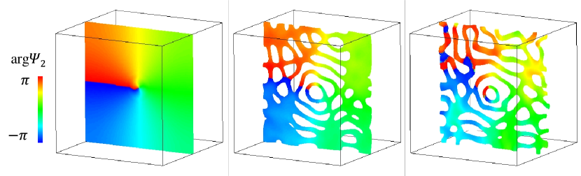
(a)                                           (b)                                           (c)

Figure 12: (Color online) A numerical simulation of a vorton creation. Surfaces are defined by $n_{1}-n_{2}=0.18(\mu_{1}/g)$ ($\mu_{1}=g=1,\hbar=m=1$), while color represents the phase of the $\Psi_{2}$ component. (a) First, we prepare a pair of a domain wall and an anti-domain wall at coincident limit with a vortex winding in the $\Psi_{2}$ component. (b) Holes are created in the wall annihilation. (c) A vorton is created in the center.

IV.3 Equivalence of the vorton to the three-dimensional skyrmion

It has been already shown in Ruostekoski:2001fc ; Battye:2001ec that 3D skyrmions are topologically equivalent to vortons in two-component BECs. In this subsection, we show it in our context of the brane-anti-brane annihilations.

In Fig. 13, the arrows denote the phase of $\Psi_{1}$ along a large loop (of the square of the dotted line) going to the boundary where $\Psi_{2}$ is zero, making a link with the vorton core. The left panel of Fig. 13 represents the phases of $\Psi_{1}$ and $\Psi_{2}$ of the vorton from the brane-anti-brane annihilation [see also Fig. 11(b)]. This is topologically equivalent to the right panel of Fig. 13. Here we show that the phase structure of the right panel is that of a 3D skyrmion. They are topologically isomorphic to each other.

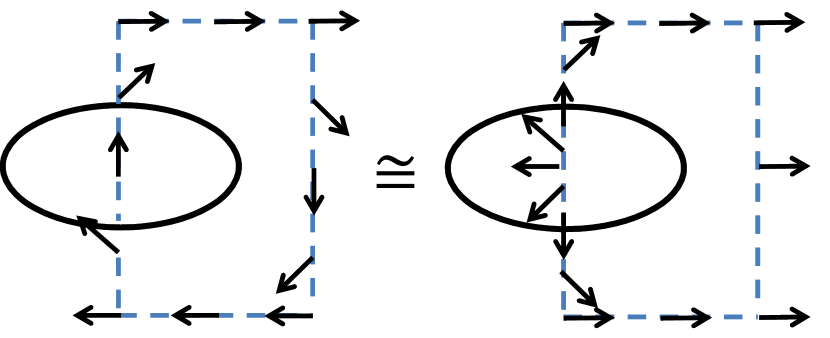
Figure 13: (Color online) The equivalence between the vorton and the 3D skyrmion. The arrows denote the phase of $\Psi_{1}$ along a large loop (of the square of the dotted line) going to the boundary where $\Psi_{2}$ is zero, making a link with the vorton core. The left panel represents the configuration of the vorton from the brane-anti-brane annihilation [see Fig. 11-(a)], while the right panel represents the configuration of a 3D skyrmion. They are topologically isomorphic to each other.

First, let us introduce the matrix $U$ as

$$\left(\begin{array}[]{c}\Psi_{1}\\ \Psi_{2}\end{array}\right)=\left(\begin{array}[]{cc}\Psi_{1}&-\Psi_{2}^{*}\\ \Psi_{2}&\Psi_{1}^{*}\end{array}\right)\left(\begin{array}[]{c}1\\ 0\end{array}\right)=U\left(\begin{array}[]{c}1\\ 0\end{array}\right),$$ (41)

with

$$U\equiv\left(\begin{array}[]{cc}\Psi_{1}&-\Psi_{2}^{*}\\ \Psi_{2}&\Psi_{1}^{*}\end{array}\right)$$ (44)

being an element of an $SU(2)$ group, when

$$\det U=|\Psi_{1}|^{2}+|\Psi_{2}|^{2}=1.$$ (45)

The GP energy functional given in Eq. (5) is not $SU(2)$ symmetric in general. When the relations

$$g_{11}=g_{22}=g_{12},\quad\mu_{1}=\mu_{2}$$ (46)

hold, the GP energy functional is $SU(2)$ symmetric, and Eq. (45) holds (up to overall constant) footnote1 .

Even when the GP energy functional given in Eq. (5) is not $SU(2)$ symmetric, we can approximately consider the parametrization by $U$ in Eq. (44). A rotationally symmetric configuration of a 3D skyrmion can be given by Skyrme:1961vq

$$U=\exp i\left(f(r){{\bf r}\over|{\bf r}|}\cdot{\bf\sigma}\right)$$ (47)

with a function $f(r)$ with the boundary condition

$$f(r=0)=n\pi,\quad f(r=R)=0,$$ (48)

where $R$ is the size of the system. Here, $n\in{\bf Z}$ is an element of the third homotopy group $\pi_{3}(SU(2))\simeq{\bf Z}$.

In the polar coordinates $(r,\theta,\phi)$,

$${{\bf r}\over|{\bf r}|}=(\sin\theta\cos\phi,\sin\theta\sin\phi,\cos\theta).$$ (49)

By using the formula, $\exp(i\Theta{\bf n}\cdot{\bf\sigma})=\cos\Theta+i{\bf n}\cdot{\bf\sigma}\sin\Theta$ for ${\bf n}^{2}=1$, the 3D skyrmion in Eq. (41) with $U$ in Eq. (47) can be obtained as

$$\left(\begin{array}[]{c}\Psi_{1}\\ \Psi_{2}\end{array}\right)=\left(\begin{array}[]{c}\cos f(r)-i\sin f(r)\cos\theta\\ \sin f(r)\sin\theta e^{-i\phi}\end{array}\right).$$ (54)

First, let us study the phase structure of $\Psi_{1}$ of the 3D skyrmion in Eq. (54). At the boundaries and the origin, Eq. (54) becomes

$$\left(\begin{array}[]{c}\Psi_{1}\\ \Psi_{2}\end{array}\right) = \left(\begin{array}[]{c}1\\ 0\end{array}\right)\mbox{ at }r=R,$$ (59)

$$\left(\begin{array}[]{c}\Psi_{1}\\ \Psi_{2}\end{array}\right) = \left(\begin{array}[]{c}(-1)^{n}\\ 0\end{array}\right)\mbox{ at }r=0.$$ (64)

Along the $x^{1}$-axis ($\theta=0,\pi$), Eq. (54) becomes

$$\left(\begin{array}[]{c}\Psi_{1}\\ \Psi_{2}\end{array}\right) = \left(\begin{array}[]{c}\exp[-if(r)]\\ 0\end{array}\right)\mbox{ at }\theta=0,$$ (69)

$$\left(\begin{array}[]{c}\Psi_{1}\\ \Psi_{2}\end{array}\right) = \left(\begin{array}[]{c}\exp[if(r)]\\ 0\end{array}\right)\mbox{ at }\theta=\pi,$$ (74)

Eqs. (64) and (74) show, in the case of $n=1$, the phase structure of $\Psi_{1}$ in the right panel of Fig. 13.

Second, let us study the phase structure of $\Psi_{2}$. We consider the ring defined by $\theta=\pi/2$ and the radius $r$ such that $f(r)=\pi/2$. Along this ring, the $\Psi_{i}$ are

$$\left(\begin{array}[]{c}\Psi_{1}\\ \Psi_{2}\end{array}\right)=\left(\begin{array}[]{c}0\\ e^{-i\phi}\end{array}\right).$$ (79)

The $\Psi_{2}$ component winds once along this ring, as in Fig. 11(c). This winding of the $\Psi_{2}$ component originates from the winding in the brane-anti-brane configuration in Eq. (32).

We thus have seen that the 3D skyrmion in Eq. (41) is topologically equivalent to a vorton.

V Summary and discussion

We have studied a mechanism to create a vorton or three dimensional skyrmion in phase separated two-component BECs. We consider a pair of a domain wall and an anti-domain wall with vortices stretched between them. The $\Psi_{2}$ component is sandwiched by the regions of the $\Psi_{1}$ component, where the phase difference of $\Psi_{1}$’s in the two separated regions is taken to be $\pi$. When the domain wall pair decays, there appear vortex loops of the $\Psi_{1}$ component with the $\Psi_{2}$ component trapped inside their cores. If a $\Psi_{1}$ vortex loop encloses one stretched vortex, it becomes a vorton. More generally, if the vortex loop encloses $n$ of the stretched vortices, it becomes a vortex ring with the phase of $\Psi_{2}$ twisted $n$ times. We also have confirmed that the vorton ($n=1$) is topologically equivalent to a 3D skyrmion.

Experimentally this can be realized by preparing the phase separation in the order $\Psi_{1}$, $\Psi_{2}$ and $\Psi_{1}$ components, and rotating the intermediate $\Psi_{2}$ component. By selectively removing the filling $\Psi_{2}$ component with a resonant laser beam, the collision of the brane and anti-brane can be made, to create vortons.

Once created in the laboratory, one can study the stability and dynamics of a vorton experimentally. The vorton will propagate along the direction perpendicular to the initial configuration of the branes. Therefore, to investigate the dynamics of a vorton, we need to prepare a large size of cloud in that direction. In the case of untwisted vortex loop (usual loop, not a vorton), it will easily shrink and eventually decay into phonons if the thermal dissipation works enough. However, the vorton should be stable against the shrinkage and will propagate to reach the surface of the atomic cloud. Such a difference must be a benchmark to detect vortons in experiments.

On the other hand, the thermal and quantum fluctuations may make the vorton unstable. Our numerical calculations rely on the mean field GP theory. The topological charge of a vorton is the winding of the phase of $\Psi_{2}$ along the closed loop (which is proportional to the superflow along the closed loop). Since this topological charge is defined only in the vicinity of the vorton, there is a possibility that it can be unwound, once quantum/thermal fluctuation is taken into account beyond the mean field theory. Quantum mechanically, such a decay is caused by an instanton effect (quantum tunneling). This process also resembles the phase slip of superfluid rings. The vorton decay by the quantum and thermal tunneling is considered to be an important process in high energy physics and cosmology, since it will radiate high energy particles such as photons, which may explain some high energy astrophysical phenomena observed in our Universe. Therefore it would be important that one realizes vortons in laboratory by using ultra-cold atomic gases; it may simulate a vorton decay with emitting phonons quantum mechanically, beyond the mean field approximation.

In this paper, we have mainly studied topological aspects of the vorton creation using the NL$\sigma$M approximation. In order to study dynamics of topological defects beyond this approximation, we need a precise form of the interaction between the defects. An analytic form of the interaction between vortices was derived in the case of miscible ($c_{2}>0$) two-component BECs, and it was applied to the analysis of vortex lattices Eto:2011wp . Extension to the case of the immiscible case ($c_{2}<0$) focused in this paper will be useful to study the interaction between vortices attached to domain walls, and that between vortons and/or walls

In our previous paper Kasamatsu:2010aq , we discussed that the domain wall in two-component BECs can be regarded as a D2-brane, as the D-brane soliton Gauntlett:2000de ; Shifman:2002jm ; Isozumi:2004vg ; Eto:2006pg ; Eto:2008mf in field theory, where “D$p$-brane” implies a D-brane with $p$ space dimensions. This is because the string endpoints are electrically charged under $U(1)$ gauge field of the Dirac-Born-Infeld (DBI) action for a D-brane Dirac:1962iy . In our context, the $U(1)$ gauge field is obtained by a duality transformation from $U(1)$ Nambu-Goldstone mode of the domain wall. Since the D-brane soliton Kasamatsu:2010aq in two-component BECs, precisely coincides with a BIon Gibbons:1997xz , i.e., a soliton solution of the DBI action of a D-brane, the domain wall can be regarded as a D2-brane.

On the other hand, it is known in string theory Sen that when a D$p$-brane and an anti-D$p$-brane annihilate on collision, there appear D$(p-2)$ branes. If we want to regard our domain wall as a D2-brane, the pair annihilation of a D2-brane and anti-D2-brane should result in the creation of D0-branes. Therefore, a discussion along this line leads us to suggest a possible interpretation of 3D skyrmions as D0-branes, which are point-like objects.

- (1) E. Witten, Nucl. Phys. B 249, 557 (1985).
- (2) R. L. Davis and E. P. S. Shellard, Phys. Lett. B 209, 485 (1988).
- (3) E. Radu and M. S. Volkov, Phys. Rept. 468, 101 (2008).
- (4) G. E. Volovik, The Universe in a Helium Droplet, Clarendon Press, Oxford (2003).
- (5) A. Vilenkin and E. P. S. Shellard, Cosmic Strings and Other Topological Defects, (Cambridge Monographs on Mathematical Physics), Cambridge University Press (July 31, 2000).
- (6) T. H. R. Skyrme, Proc. Roy. Soc. Lond. A 260, 127 (1961); Nucl. Phys. 31, 556 (1962).
- (7) N. S. Manton and P. Sutcliffe, Topological solitons, Cambridge, UK: Univ. Pr. (2004) 493 p
- (8) J. Ruostekoski and J. R. Anglin, Phys. Rev. Lett. 86, 3934 (2001).
- (9) R. A. Battye, N. R. Cooper and P. M. Sutcliffe, Phys. Rev. Lett. 88, 080401 (2002).
- (10) U. A. Khawaja and H. T. C. Stoof, Nature (London) 411, 918 (2001), Phys. Rev. A 64, 043612 (2001).
- (11) C. M. Savage and J. Ruostekoski, Phys. Rev. Lett. 91, 010403 (2003).
- (12) J. Ruostekoski, Phys. Rev. A 70, 041601 (2004).
- (13) S. Wuster, T. E. Argue, and C. M. Savage, Phys. Rev. A 72, 043616 (2005).
- (14) I. F. Herbut and M. Oshikawa, Phys. Rev. Lett. 97, 080403 (2006); A. Tokuno, Y. Mitamura, M. Oshikawa, I. F. Herbut, Phys. Rev. A 79, 053626 (2009).
- (15) M. A. Metlitski and A. R. Zhitnitsky, JHEP 0406, 017 (2004).
- (16) P. F. Bedaque, E. Berkowitz and S. Sen, arXiv:1111.4507 [cond-mat.quant-gas].
- (17) L. S. Leslie, A. Hansen, K. C. Wright, B. M. Deutsch, and N. P. Bigelow, Phys. Rev. Lett. 103, 250401 (2009); J. Choi, W. J. Kwon, and Y. Shin Phys. Rev. Lett. 108, 035301 (2012).
- (18) H. T. C. Stoof, E. Vliegen, and U. Al Khawaja, Phys. Rev. Lett. 87, 120407 (2001).
- (19) J. -P. Martikainen, A. Collin, and K. -A. Suominen, Phys. Rev. Lett. 88, 090404 (2002).
- (20) C. M. Savage and J. Ruostekoski, Phys. Rev. A 68, 043604 (2003).
- (21) V. Pietilä and M. Möttönen, Phys. Rev. Lett. 103, 030401 (2009).
- (22) Y. Kawaguchi, M. Nitta and M. Ueda, Phys. Rev. Lett. 100, 180403 (2008).
- (23) G. W. Semenoff and F. Zhou, Phys. Rev. Lett. 98, 100401 (2007); M. Kobayashi, Y. Kawaguchi, M. Nitta and M. Ueda, Phys. Rev. Lett. 103, 115301 (2009).
- (24) K. Kasamatsu, M. Tsubota and M. Ueda, Int. J. Mod. Phys. B 19, 1835 (2005); Y. Kawaguchi, M. Kobayashi, M. Nitta and M. Ueda, Prog. Theor. Phys. Suppl. 186, 455 (2010) M. Ueda and Y. Kawaguchi, arXiv:1001.2072 (2010).
- (25) G. Thalhammer, et al. Phys. Rev. Lett. 100, 210402 (2008).
- (26) S. B. Papp, J. M. Pino, and C. E. Wieman, Phys. Rev. Lett. 101, 040402 (2008).
- (27) K. Kasamatsu, M. Tsubota, and M. Ueda, Phys. Rev. A 71, 043611 (2005).
- (28) E. Babaev, L. D. Faddeev and A. J. Niemi, Phys. Rev. B 65, 100512 (2002).
- (29) E. Babaev, Phys. Rev. B 79, 104506 (2009).
- (30) J. P. Gauntlett, R. Portugues, D. Tong and P. K. Townsend, Phys. Rev. D 63, 085002 (2001).
- (31) M. Shifman and A. Yung, Phys. Rev. D 67, 125007 (2003).
- (32) Y. Isozumi, M. Nitta, K. Ohashi and N. Sakai, Rev. D 71, 065018 (2005).
- (33) M. Eto, Y. Isozumi, M. Nitta, K. Ohashi and N. Sakai, J. Phys. A A 39, R315 (2006).
- (34) M. Eto, T. Fujimori, T. Nagashima, M. Nitta, K. Ohashi and N. Sakai, Phys. Rev. D 79, 045015 (2009).
- (35) J. Polchinski, Phys. Rev. Lett. 75, 4724 (1995).
- (36) R. G. Leigh, Mod. Phys. Lett. A4, 2767 (1989).
- (37) J. Polchinski, String Theory (Cambridge Univ. Press, Cambridge, 1998).
- (38) K. Kasamatsu, H. Takeuchi, M. Nitta and M. Tsubota, JHEP 1011, 068 (2010).
- (39) M. O. Borgh and J. Ruostekoski, arXiv:1202.5679 [cond-mat.quant-gas].
- (40) D. I. Bradley, S. N. Fisher, A. M. Guénault, R. P. Haley, J. Kopu, H. Martin, G. R. Pickett, J. E. Roberts and V. Tsepelin, Nature Phys. 4, 46 (2008).
- (41) B. P. Anderson, P. C. Haljan, C. A. Regal, D. L. Feder, L. A. Collins, C. W. Clark, and E. A. Cornell, Phys. Rev. Lett. 86, 2926 (2001).
- (42) H. Takeuchi, K. Kasamatsu, M. Nitta and M. Tsubota, J. Low Temp. Phys. 162, 243 (2011); H. Takeuchi, K. Kasamatsu, M. Tsubota and M. Nitta, arXiv:1205.2330 [cond-mat.quant-gas].
- (43) C. J. Pethick and H. Smith, Bose-Einstein Condensation in Dilute Gases, 2nd ed. (Cambridge Univ. Press, Cambridge, 2008).
- (44) A. Sen, Int. J. Mod. Phys. A 20, 5513 (2005).
- (45) P. W. Anderson and G. Toulouse, Phys. Rev. Lett. 38, 508 (1977).
- (46) A. M. Polyakov and A. A. Belavin, JETP Lett. 22, 245 (1975) [Pisma Zh. Eksp. Teor. Fiz. 22, 503 (1975)].
- (47) In the symmetric case, the conditions in Eq. (46) imply in the NLM description, and consequently there is no potential. By noting the isomorphism , the target space is a quotient of by gauge symmetry: , which is nothing but the Hopf fiberation.
- (48) M. Eto, K. Kasamatsu, M. Nitta, H. Takeuchi and M. Tsubota, Phys. Rev. A 83, 063603 (2011); P. Mason and A. Aftalion, Phys. Rev. A 84, 033611 (2011); A. Aftalion, P. Mason, and J. Wei, Phys. Rev. A 85, 033614 (2012).
- (49) P. A. M. Dirac, Proc. Roy. Soc. Lond. A 268, 57 (1962); M. Born and L. Infeld, Proc. Roy. Soc. Lond. A 144, 425 (1934).
- (50) G. W. Gibbons, Nucl. Phys. B 514, 603 (1998). C. G. Callan and J. M. Maldacena, Nucl. Phys. B 513, 198 (1998).