A 1D modelling of streaming potential dependence on water content during drainage experiment in sand

Abstract

The understanding of electrokinetics for unsaturated conditions is crucial for numerous of geophysical data interpretation. Nevertheless, the behaviour of the streaming potential coefficient $C$ as a function of the water saturation $S_{w}$ is still discussed. We propose here to model both the Richards equation for hydrodynamics and the Poisson’s equation for electrical potential for unsaturated conditions using 1D finite element method. The equations are first presented and the numerical scheme is then detailed for the Poisson’s equation. Then, computed streaming potentials (SP) are compared to recently published SP measurements carried out during drainage experiment in a sand column. We show that the apparent measurement of $\Delta V/\Delta P$ for the dipoles can provide the streaming potential coefficient in these conditions. Two tests have been performed using existing models for the SP coefficient and a third one using a new relation. The results show that existing models of unsaturated SP coefficients $C(S_{w})$ provide poor results in terms of SP magnitude and behaviour. We demonstrate that the unsaturated SP coefficient can be until one order of magnitude larger than $C_{sat}$, its value at saturation. We finally prove that the SP coefficient follows a non-monotonous behaviour with respect to water saturation.

1 Introduction

Electric and electromagnetic methods are used in a large range of geophysical applications because of their sensitivity to fluids within the crust. The electrical resistivity can be related to the permeability and to the deformation, in full-saturated or in partially-saturated conditions (Doussan & Ruy, 2009; Henry et al., 2003; Jouniaux et al., 1994, 2006). The self-potentials have also been successfully used in the last decades. Self-potentials have been observed to detect contaminant plumes or salted fronts through the interpretation of electrochemical effects (Naudet et al., 2003; Maineult et al., 2006b, a). Most of the self-potential observations are interpreted through the electrokinetic effect. It has been proposed to use this electrokinetic effect for the seismic prediction (Fenoglio et al., 1995; Pozzi & Jouniaux, 1994). For hydrological applications, some hydraulic properties can be inferred from the self-potential observations (Gibert & Pessel, 2001; Sailhac et al., 2004; Glover et al., 2006; Glover & Walker, 2009). The W-shaped anomalies classically observed on active volcanoes are used to characterize geothermal circulations (Finizola et al., 2002, 2004; Saracco et al., 2004; Mauri et al., 2010; Onizawa et al., 2009). It has also been proposed to use the self-potential monitoring to detect at distance the propagation of a water front in a reservoir (Saunders et al., 2008). Moreover self-potentials have been monitored during hydraulic tests in boreholes leading to some relationship with the microseismicity (Darnet et al., 2006), and showing a non-linear behaviour that could be related to the saturation and desaturation processes (Maineult et al., 2008). Streaming potential (SP) results from the coupling between fluid (water) flow and electrical current, through the motion of ionic charges of water in the pore space. The distribution of ions near the matrix surface is described by the electric double layer, including the diffuse layer in which the number of counterions exceeds the number of cations adsorbed to the matrix (Davis et al., 1978). The streaming current is caused by the motion of ions from the diffuse layer, coming from a pressure difference. This current is then balanced by a conduction current leading to the SP.
In steady state flows through homogeneous media, one can define the streaming potential coefficient $C$ as the ratio between the measured electrical potential difference $\Delta V$ and the driving pore water pressure difference $\Delta P$ (Overbeek, 1952). The streaming potential is a function of various parameters, and its dependence on water salinity (Ishido & Mizutani, 1981; Jaafar et al., 2009; Vinogradov et al., 2010), water electrical conductivity (Pride & Morgan, 1991; Lorne et al., 1999), pH (Ishido & Mizutani, 1981; Guichet et al., 2006) or temperature (Tosha et al., 2003) is still studied.
However, one is forced to notice a lake of data concerning the SP coefficient dependence on water content. For shallow surface geophysical applications, including also the seismoelectric conversions (Dupuis et al., 2007) which is studied in laboratory (Bordes et al., 2006, 2008), a better understanding of electrokinetics for unsaturated conditions is needed. A way for the understanding of such a phenomena is to study the streaming potential coefficient as a function of saturation.
The first experimental SP coefficient measurements were performed by Guichet et al. (2003). These authors measured SP during drainage experiments performed by injecting inert gas through sand, and inferred a linear relation between the relative SP coefficient $C_{r}$ (i.e $C$ normalized by its value at saturation $C_{sat}$) and effective water saturation $S_{e}$. Perrier & Morat (2000) proposed an empirical expression to explain the dependence of $C_{r}$ on water content based on a relative permeability model. The implicit assumption was that the electrical currents are affected by unsaturated state in a comparable way than hydrological flow. Revil et al. (2007) proposed recently another formula to characterize this dependence also based on a relative permeability model. Linde et al. (2007) proposed another expression to model some SP measurements performed during a drainage experiment, with similar conditions to those from Allègre et al. (2010). However, these studies do not provide a combined hydrodynamic and electrical approach to model the data, as it should be done. For reservoir applications Saunders et al. (2008) proposed a linear expression for $C_{r}$ in the case of oil imbibition. All these models predict a monotonous decrease of $C_{r}$ with decreasing water saturation. Recently, Allègre et al. (2010) proposed original SP measurements performed during a drainage experiment and measured the first continuous recordings of the SP coefficient as a function of water saturation. They observed that the SP coefficient exhibits two different behaviours as the water saturation decreases. Values of $C_{r}$ first increase for decreasing saturation in the range $0.55-0.8<S_{w}<1$, and then decrease from $S_{w}=0.55-0.8$ to residual water saturation. This behaviour was never reported before and called for new interpretations of electrokinetic phenomena for unsaturated conditions.
Streaming potentials have been successfully modelled for aquifer properties determination (Darnet et al., 2003) or for water infiltration conditions (Sailhac et al., 2004). Sheffer & Oldenburg (2007) proposed a 3D modelling of streaming potential at the field scale for saturated conditions. Jackson (2010) used a bundle capillary model to compute the SP coefficent as a function of water-saturation. He showed that the behaviour of the SP coefficient depends on the capillary size distribution, the wetting behaviour of the capillaries, and whether we invoke the thin or thick electrical double layer assumption. Depending upon the chosen value of the saturation exponent and the irreductible water-saturation, the relative SP coefficient may increase at partial saturation, before decreasing to zero at the irreductible saturation.
Finally, no previous study took into account hydrodynamics and electrical potential equations together, even in a simple geometry, to model the streaming potential coefficient for unsaturated conditions. Thus, we propose here to model SP by solving both the Richards equation for hydrodynamics and the Poisson’s equation for electrical potential using 1D finite element method. Existing models which describe the behaviour of $C_{r}$ as a function of $S_{e}$ are tested and compared to a new expression inferred from SP measurements by Allègre et al. (2010). Thus, after introducing governing equations, computed SP using these models are presented and compared to measurements. The results lead to the conclusions that 1) a non-monotonous behaviour of $C_{r}$ is required to fit the measurements; 2) The apparent measurement of $\Delta V/\Delta P$ for the dipoles can provide the streaming potential coefficient in these conditions.

2 Governing equations

2.1 Hydrodynamic equations

Combining the mass conservation equation to the 1D generalized Darcy’s law leads to the mixed form of the Richards equation (Richards, 1931), which describes unsaturated flow in porous media,

$$\frac{\partial\theta(h)}{\partial t}-\frac{\partial}{\partial z}\left[K(h)\left(\frac{\partial h}{\partial z}-1\right)\right]=0$$ (1)

where $\theta(h)$ is the volumetric water content [m³.m^-3], dependent on the pressure head $h$ [m]. The parameter $K$, which is also a function of the pressure head, is the hydraulic conductivity [m.s^-1], $t$ is time [s], and $z$ is the vertical coordinate [m] taken to be positive downward. The dependence of the hydraulic conductivity and pressure head on water content is non-linear. Numerous retention and relative permeability models are able to take into account this dependence (Gardner, 1958; Brooks & Corey, 1964; van Genuchten, 1980). The models which have been chosen for this work were proposed respectively by Brooks & Corey (1964),

$$Se=\frac{\theta-\theta_{r}}{\theta_{s}-\theta_{r}}=\left\{\begin{array}[]{l}{{\left(\dfrac{h_{a}}{|h|}\right)^{\lambda}}~{}~{},\text{if}~{}~{}\dfrac{h_{a}}{|h|}<1}\\ {1~{}~{},\text{if}~{}~{}\dfrac{h_{a}}{|h|}>1}\end{array}\right.$$ (2)

and Mualem (1976),

$$K(S_{e})={K_{s}}.{S_{e}}^{L+2+\frac{2}{\lambda}}$$ (3)

with $S_{e}$ the effective water saturation, $\theta_{s}$ the water content at saturation [m³.m^-3], also equal to porosity $\phi$, $\theta_{r}$ the residual water content [m³.m^-3], and $K_{s}$ the hydraulic conductivity at saturation [m.s^-1]. The effective water saturation can be expressed by: $S_{e}=(S_{w}-S_{w}^{r})/(1-S_{w}^{r})$, with $S_{w}$ ($S_{w}=\theta/\phi$) and $S_{w}^{r}$ ($S_{w}^{r}=\theta_{r}/\phi$) the water saturation and the residual water saturation respectively. The parameter $\lambda$ in equation 2 is a measure of the pore size distribution and characterizes the medium granulometry. Thus, higher the value of $\lambda$ is, higher homogeneous the medium is. The second hydrodynamic parameter $h_{a}$ is the air entry pressure (Brooks & Corey, 1964). The last parameter $L$ takes into account the tortuosity and is chosen as $L=0.5$, which is a common value in the literature (Mualem, 1976).
Some initial and boundary conditions are necessary to solve the Richards equation. Initial condition is a saturated sand at the hydrostatic equilibrium, so that the water pressures (expressed in cm of water) at the top and the bottom boundary of the system are respectively $h(z=0)=0$ and $h(z=l)=l$. Considering the drainage experiment which will be presented in this work, two conditions have been used. The first one is a zero flux $q_{0}(t)$ at the top of the system (Neumann type) and the second one is a constant pressure head $h_{l}(t)$ at the bottom (Dirichlet type). These conditions are written as,

$$h(z=l,t)=h_{l}(t)\ \ {\text{and}}\ \ \left(-K(h)\frac{\partial h}{\partial z}+K\right)_{z=0}=q_{0}(t)$$ (4)

where $z=0$ or $z=l$ and $l$ the length of the system. The Richards equation has been discretized using the Galerkin finite element method (Pinder & Gray, 1977), with a fully implicit scheme in time. To take into account dependency between $h$, $\theta$ and $K$, the equation is linearized using the Newton-Raphson method. This approach has been used for decades to solve this equation, and the detailed scheme can be found for example in Lehmann & Ackerer (1998).

2.2 Electrokinetic theory

Coupled fluxes can be described by the general equation,

$$\mathbf{J}_{i}=\sum_{j=1}^{N}{\cal{L}}_{ij}\mathbf{X}_{j}$$ (5)

which link the forces $\mathbf{X}_{j}$ to macroscopic fluxes $\mathbf{J}_{i}$, through transport coupling coefficients ${\cal{L}}_{ij}$ (Onsager, 1931). The global SP field can be described as the sum of several contributions creating electrical current sources. These current sources derive from macroscopic potentials, through electrochemical effects (e.g. concentration gradients), electrokinetics (e.g. electrical potential gradients, electro-osmosis) or thermo-electrical effects (e.g. temperature gradients). Considering some of these potential fields, the total electrical current density can be written as:

$${\bf{J}}=-{\cal{L}}_{T}\dfrac{\boldsymbol{\nabla}T}{T}+\boldsymbol{\nabla}\Phi_{J}+{\cal{L}}_{e}\boldsymbol{\nabla}V-{\cal{L}}_{ek}\boldsymbol{\nabla}P,$$ (6)

where $T$ is the temperature [K], ${\cal{L}}_{T}=-T\pi\sigma_{T}$ [W.m.s^-1] is given by the Peltier effect, $\Phi_{J}$ is the junction potential [V], which also can be expressed as a function of chemical concentration gradients in electrolytes ($\boldsymbol{\nabla}C_{c}/C_{c}$) by $\boldsymbol{\nabla}\Phi_{J}=\alpha_{m}\boldsymbol{\nabla}C_{c}/C_{c}$, with $\alpha_{m}$ the fluid junction coupling coefficient (Naudet et al., 2003; Maineult et al., 2008; Jouniaux et al., 2009). The parameter $V$ is the electrical potential [V], thus Ohm’s law identify ${\cal{L}}_{e}=-\sigma_{r}$, with $\sigma_{r}$ the bulk electrical conductivity [S.m^-1]. The last term of equation 6 describes electrokinetic effects created by the driving pressure gradient $\boldsymbol{\nabla}P$, through the electrokinetic coupling ${\cal{L}}_{ek}$, defined as ${\cal{L}}_{ek}\equiv-\sigma_{r}C$ [A.Pa^-1.m^-1] (Pride, 1994). The parameter $C$ [V.Pa^-1] is known as the SP coefficient. The total water pressure P can be inferred from water pressures $h$ with: $P=\rho_{w}g(h-z)$, where $\rho_{w}$ is the water density [kg.m^-3], g is gravity and $z$ is the vertical location taken to be positive downward.
Considering a constant temperature, and no concentration gradients, one can write the following coupled equation:

$${\bf{J}}={\cal{L}}_{e}{\boldsymbol{\nabla}}V-{\cal{L}}_{ek}{\boldsymbol{\nabla}}P,$$ (7)

$$\text{or},$$

$${\bf{J}}=-\sigma_{r}{\boldsymbol{\nabla}}V+\sigma_{r}C{\boldsymbol{\nabla}}P.$$ (8)

Without any external current sources, the conservation of the total current density implies,

$${\boldsymbol{\nabla}}\cdot\mathbf{J}=0.$$ (9)

In the case of heterogeneous medium, one can assume for example a tabular medium with electrical conductivity and SP coefficient contrasts, then equation 8 through 9 leads to the following Poisson’s equation:

$$\boldsymbol{\nabla}\cdot\mathbf{J}=-\sigma_{r}\boldsymbol{\nabla}^{2}V-\boldsymbol{\nabla}V\cdot\boldsymbol{\nabla}\sigma_{r}+\boldsymbol{\nabla}(C\sigma_{r})\cdot\boldsymbol{\nabla}P+\sigma_{r}C\boldsymbol{\nabla}^{2}P=0.$$ (10)

In addition to primary current sources occuring from the term $\sigma_{r}C\boldsymbol{\nabla}^{2}P$, some secondary sources linked to the term $\boldsymbol{\nabla}(C\sigma_{r})\cdot\boldsymbol{\nabla}P$ appear. These sources are located at boundaries formed by electrical conductivity and SP coefficient constrasts.
In the case of an homogeneous medium and without any contrasts of $\sigma_{r}$ and $C$, the equation 10 reduces to:

$$\boldsymbol{\nabla}^{2}V=C\boldsymbol{\nabla}^{2}P.$$ (11)

Considering for example a steady-state saturated flow through a capillary the SP coefficient $C$ [V.Pa^-1] can be expressed as the ratio between the SP difference $\Delta V$ [V] and the driving-pressure difference $\Delta P$ [Pa],

$$C=\frac{\Delta V}{\Delta P}.$$ (12)

In one dimension, the equation 9 can be written as,

$$\frac{\partial}{\partial z}\left(-\sigma_{r}\frac{\partial V}{\partial z}\right)+\frac{\partial}{\partial z}\left[{\rho_{w}g\cal{L}}_{ek}\left(\dfrac{\partial h}{\partial z}-1\right)\right]=0.$$ (13)

2.3 Discretization of the Poisson’s equation

The Poisson’s equation was solved using 1D finite element method. A first order basis function $\phi(z)$ has been chosen to discretize the Poisson’s equation. This choice implies that variables and coefficients of the equation 13 vary linearly in each element. For each node $i$ of the system, the basis function is written $\phi_{i}(z)$. Then, the equation which has to be solved can be written as,

$$\int_{0}^{l}\frac{\partial}{\partial z}\left(-\sigma_{r}\frac{\partial V}{\partial z}\right)\phi(z)dz$$

$$+\int_{0}^{l}\frac{\partial}{\partial z}\left[\rho_{w}g{\cal{L}}_{ek}\left(\dfrac{\partial h}{\partial z}-1\right)\right]\phi(z)dz=0.$$ (14)

Using this method, all variables and coefficients are approximated on each element using the same basis function:

$$V(z,t)=\sum_{1}^{ne}V_{i}(t)\phi_{i}(z),$$ (15)

$$h(z,t)=\sum_{1}^{ne}{h}_{i}(t)\phi_{i}(z),$$ (16)

$${\cal{L}}_{ek}(z,t)=\sum_{1}^{ne}{{\cal{L}}_{ek}}_{i}(t)\phi_{i}(z),$$ (17)

$$\sigma_{r}(z,t)=\sum_{1}^{ne}{\sigma_{r}}_{i}(t)\phi_{i}(z),$$ (18)

where $nn=ne+1$ is the number of nodes in the system of length $l$, and $ne$ the number of elements. The $V_{i}(t)$, ${h}_{i}(t)$, ${{\cal{L}}_{ek}}_{i}(t)$ and ${\sigma_{r}}_{i}(t)$ are respectively the values of the electrical potential, water pressure, electrokinetic coupling and bulk electrical conductivity at node $i$. For notations simplicity ${{\cal{L}}_{ek}}_{i}(t)$ will be written ${\cal{L}}_{i}(t)$ in the following. After integrating by parts equation 14, the final system of equation to be solved is given by,

$$[A].V_{i}=-[B].h_{i}-\{F_{j}\},$$ (19)

where the elements of [A], [B] and vector $\{F_{j}\}$ can be deduced from the following integrals:

$$A_{ij}=\int_{0}^{l}\left(\sum_{k=1}^{nn}\phi_{k}\ \sigma_{k}\right)\phi^{{}^{\prime}}_{i}\phi^{{}^{\prime}}_{j}dz,$$ (20)

$$B_{ij}=\rho_{w}g\int_{0}^{l}\left(\sum_{k=1}^{nn}\phi_{k}\ {\cal{L}}_{k}\right)\phi^{{}^{\prime}}_{i}\phi^{{}^{\prime}}_{j}dz,$$ (21)

$$F_{j}=\rho_{w}g\int_{0}^{l}\left(\sum_{k=1}^{nn}\phi_{k}\ {\cal{L}}_{k}\right)\phi^{{}^{\prime}}_{j}dz.$$ (22)

The matrices [A] is tridiagonal and the system can be solved using Thomas algorithm (Press et al., 1992). The system introduced in equation 19 can be detailed for each element $i$ as:

$$\dfrac{1}{2\Delta z}\left[-(\sigma_{i-1}+\sigma_{i}).V_{i-1}+(\sigma_{i-1}+2\sigma_{i}+\sigma_{i+1}).V_{i}\right.$$

$$\left.-(\sigma_{i}+\sigma_{i+1}).V_{i+1}\right]=\dfrac{\rho_{w}g}{2\Delta z}\left[({\cal{L}}_{i-1}+2{\cal{L}}_{i})+{\cal{L}}_{i+1}).h_{i}\right.$$

$$\left.-({\cal{L}}_{i-1}+{\cal{L}}_{i}).h_{i-1}-({\cal{L}}_{i}+{\cal{L}}_{i+1}).h_{i+1}+({\cal{L}}_{i-1}+{\cal{L}}_{i+1})\right]$$ (23)

where $\Delta z=0.1$ cm is the spatial discretization. Boundary conditions at nodes $1$ and $nn$ are:

$$\sigma_{1}\dfrac{\partial V}{\partial z}\phi_{1}=-j_{0}$$ (24)

$$\sigma_{nn}\dfrac{\partial V}{\partial z}\phi_{nn}=-j_{l}$$ (25)

with $j_{0}$ and $j_{l}$ are the values of the current density at the top and the bottom of the system respectively. The Poisson’s equation is solved in terms of electrical potential $V$. Thus, two boundary conditions are necessary: one on the total current density $J$ (Neumann type) and one on the electrical potential itself $V$ (Dirichlet type). As no current outflow can occur at the top and the bottom of the system (i.e no electrical exchange between the medium and the air), the total current density $j_{0}$ at $z=0$ and $z=l$ are: $j_{0}=j_{l}=0$ A.m^-2. In addition, a constant value of electrical potential $V_{0}$ has been chosen at the top of the system. This constant can be a reference value, so that $V_{0}=0$ V has been chosen for simplicity.
The modelling process is carried out using the following protocol: 1. Considering hydrodynamic boundary conditions, the equation 1 is first solved, so that water pressures and corresponding water contents are computed at each node and each time step; 2. The Poisson’s equation is then solved using equation 19, which allows to compute the electrical potential at each node of the system. 3. Thus, the needed potential differences can be deduced from the computed electrical potential field and compared to measurements. The next section presents a test performed considering a linear water pressure profile in saturated conditions, i.e simulating a Darcy’s experiment. The following sections go into the unsaturated case and present computed SP differences and measurements in the case of a drainage experiment. Several hypotheses on SP coefficient dependence on water content will be considered and compared.

3 Saturated flow modelling

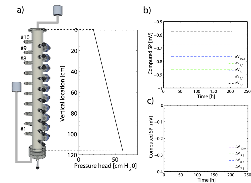
Figure 1: a) The water pressure profile used for the Darcy’s experiment simulation. The pressure head boundary conditions are constant and equal to $h_{0}=20$ cm and $h_{l}=60$ cm of equivalent water height at the top and the bottom of the column respectively. b) Computed SP between the first five electrodes (#10 to #6) and the reference #1. c) Computed SP for the dipoles (10,9), (9,8), (8,7) and (7,6). The computed values are $\Delta V{i,i-1}=-0.0954$ mV and $\Delta P{i,i-1}=59.67$ Pa which lead to $C_{sat}=1.6\times$10^-6 V.Pa^-1.

The first step is to test the code accuracy by modelling a saturated flow through a column of sand ($l=1.16$ meter height), i.e a Darcy’s experiment. The complete scheme described above was applied, so that equations 1 and 10 were solved. The water electrical conductivity $\sigma_{w}$ and saturated SP coefficient $C_{sat}$ corresponding to this test are those of Allègre et al. (2010) and are reported in Table 1. A linear and steady-state water pressure profile was applied to the medium (Figure 1a). Thus, boundary conditions at the top and the bottom of the column are constant water pressure head and given by: $h_{0}(t)=20$ cm and $h_{l}(t)=60$ cm. In this case the medium remains saturated, so that $S_{w}=1$. The boundary conditions for Poisson’s equation was a zero current density $J_{0}$ at the top and a constant electrical potential $V_{0}=$0 V at the bottom of the column. The first simulated electrode (#10) is located at 11 cm from the top of the system, while other electrodes are placed each 10 cm along it. The SP are then computed between the first five electrodes (#10 to #6) and the reference electrode (#1 15 cm above column’s bottom) and for each dipole formed by two consecutive electrodes (e.g $\Delta V_{10,9}$ will be the computed electrical potential difference between electrodes #10 and #9). The simulation were performed for 200 hrs, and the same results were obtained at each time step.
The SP differences computed between each electrode and the reference are different. This is coherent with the increasing size of each dipole, so that larger the dipole is, larger the SP difference is (Figure 1b). As the medium is homogeneous (fully saturated) SP differences computed for each dipole are merged (Figure 1c) and exhibit the value $\Delta V_{i,i-1}=-0.0954$ mV. The corresponding driving pore pressure difference for each dipole is $\Delta P_{i,i-1}=59.67$ Pa. Considering these values, the inferred SP coefficient at saturation computed with equation 12 is: $C_{sat}=-$ 1.6$\times$10^-6 V.Pa^-1. This value is exactly equal to the original $C_{sat}$ (see Table 1) used for calculation. This test experiment was performed using others water pressure profiles, other $C_{sat}$ values and other boundary condition value $V_{0}$ and always yielded to the original $C_{sat}$. We therefore confirm that the apparent measurement of $\Delta V/\Delta P$ for the dipoles can provide the streaming potential coefficient for saturated conditions.

4 Drainage experiment

4.1 Unsaturated flow modelling

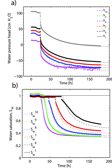
Figure 2: a) Measured (dots) and computed (dashed lines) water pressure heads deduced from the Richards equation solving. Indices $i$ indicates the location of measurement, as $h_{10}$ is the pressure head 16 cm from the column top and $h_{1}$ 10 cm from the column bottom. Other $h$ values are measured and computed each 10 cm. b) Measured (dots) and computed (dashed lines) water saturations deduced from the Richards equation solving, where indices $i$ indicates the location of measurement. The drainage starts at $t\simeq 22$ hr.

We propose to model the SP measurements of a drainage experiment carried out by Allègre et al. (2010). The SP were measured during a drainage experiment performed in a column of plexiglass of approximately 1.2 metre height and 10 cm diameter fullfilled with clean Fontainebleau sand. A constant water pressure applied at the bottom of the column allowed the drainage to start. Allègre et al. (2010) combined SP measurements to water content and water pressure measurements each 10 cm along the column. The aim of this section is to computed SP using the numerical scheme described above, considering several hypotheses for the SP coefficient dependence on water content. Thus, formula for $C_{r}$ of Guichet et al. (2003), Revil et al. (2007) and a new empirical model will be implemented to solve the Poisson’s equation.
At the beginning of the experiment, the medium is fully saturated, so that the water pressure profile is hydrostatic. The drainage starts when the boundary condition at the bottom of the column is set to a value of $h=2$ cm of equivalent water height (i.e $p_{w}(z=l)\simeq$ 200 Pa). The water pressure heads and water contents are computed at each time step by solving the equation 1 and are compared to experimental data (Figure 2). The parameters of the retention model (eq. 2) and the relative permeability model (eq. 3) are reported in Table 2. Since pressure sensors are located each ten centimetre along the column, before the drainage start, the pressure heads measurements are shifted from 10 cm between each other. These measurements are characteristics for the hydrostatic equilibrium. After the drainage start, the measured pressure heads decrease all at the same time and stabilize at different values depending on the sensor location. This shift of the pressure values at the end of the experiment (e.g at t$\simeq$ 150 h) indicates the presence of a capillary fringe and of a water saturation gradient (see Figure 2b). For very long time (around 90 days for the sand used) the water phase equilibrates itself in the column until a linear water pressure profile is reached. From the drainage start, the water saturations do not decrease at the same time, but one after the other depending on the measurement location. The time shift between the water content measurements informs on the dynamic of the saturation front propagation during the drainage experiment.
The hydrodynamic parameters used in the Richards’ equation (Table 2) were computed by inversion of the water pressure heads and water content measurements. The detailed inverse problem procedure can be found in Hayek et al. (2008). It is shown that this approach provides good estimations and small errors on $\theta_{s}$, $\lambda$ and $h_{a}$.

4.2 Unsaturated SP modelling

To solve the Poisson’s equation at each time step, a model for the SP coefficient dependence on water saturation is needed. Guichet et al. (2003) proposed that the SP coefficient vary linearly with the effective water saturation,

$$C_{r}=S_{e}.$$ (26)

Revil et al. (2007) had a different approach and proposed another relation depending on a relative permeability model as,

$$C_{r}=\dfrac{k_{r}}{S_{w}^{n+1}}~{}~{}\text{with}~{}~{}k_{r}=S_{e}^{L+2+2/\lambda},$$ (27)

where $n$ is the Archie’s saturation exponent (Archie, 1942). The $L$ parameter is usually chosen as $L=$0.5 (Mualem, 1976), but is equal to 1 in Revil et al. (2007), so that the two cases will be tested in the following. These two models have in common to predict the maximum of the SP coefficient to be $C_{sat}$ (for $S_{w}=1$). Moreover, they imply a monotonous decrease of the relative SP coefficient with decreasing saturation. Allègre et al. (2010) recently observed that $C_{r}$ could be until 200 times larger than $C_{sat}$, and that it first increases with decreasing saturation, and then decreases up to the residual water saturation. So that, we propose an empirical relation for the SP coefficient inferred from these measurements written as,

$$C=C_{sat}S_{e}[1+\beta(1-S_{e})^{\gamma}]$$ (28)

where $\beta$ and $\gamma$ are two fitted parameters. Note that $\beta$ depends on the considered dipole and varies as a function of the vertical location. This assumption coming from the experimental SP coefficients, which exhibit different maximum values, will be discussed in the following section. Contrary to the two first relations, this model predicts a non-monotonous behaviour of the SP coefficient as a function of water saturation. The three presented models were used to compute $C(S_{e})$ from computed water saturations, to solve the Poisson’s equation.
Moreover, an a priori is needed for the electrical conductivity $\sigma_{r}(S_{w})$ to solve equation 10. The electrical conductivity is inferred at each time step using the Archie’s law (Archie, 1942),

$$\sigma_{r}=\sigma_{w}\phi^{m}S_{w}^{n}$$ (29)

with $m$ and $n$ the two Archie’s exponent, $\sigma_{w}$ the water electrical conductivity [S.m^-1] and $\phi$ the porosity. The relation $C(S_{e})$ is also computed at each time step and for each element of the system from computed water saturations. All parameters’ values needed for computation are reported in Tables 2 and 3. Using the computed electrical potential values in the column, SP were computed for the dipoles (10,9), (9,8), (8,7) and (7,6), which are the dipoles located in the unsaturated part of the column during the drainage experiment.

5 Discussion

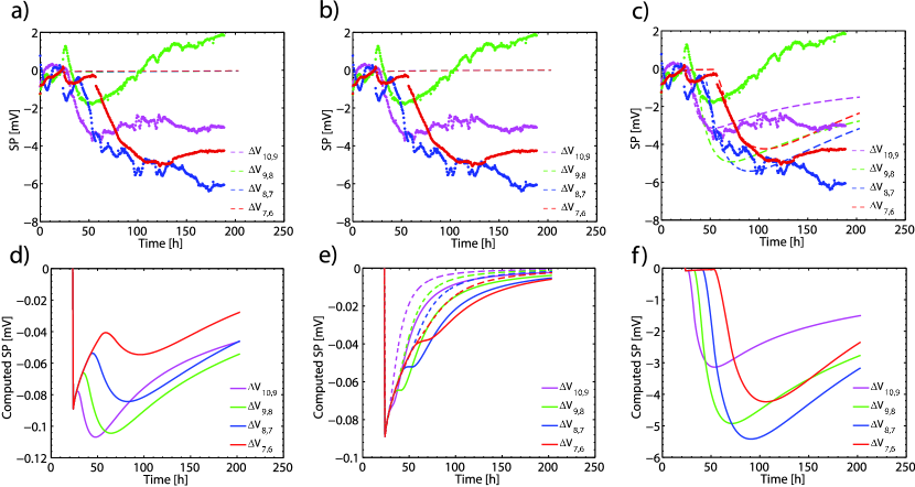
Figure 3: Measured (dots) and computed (lines) streaming potentials deduced from the Poisson’s equation solving, for each dipole, using respectively equations 26 (a), 27 (b) and 28 (c). Computed SP using equations 26 (d), 27 (e) and 28 (f) in the Poisson’s equation, and parameters from tables 2 and 3. The Revil et al. (2007) model (e) has been implemented using $L=$0.5 (lines) and $L=$1 (dashed lines).

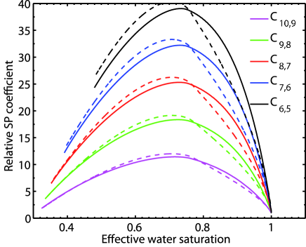
Figure 4: Computed relative SP coefficients using eq. (12) with computed $\Delta V$ and $\Delta P$ after Poisson’s equation was solved (lines), and using eq. (28) (dashed lines), for five locations in the column.

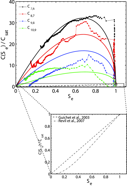
Figure 5: (On the top) Experimental SP coefficients $\Delta$V / $\Delta$P from Allègre et al. (2010) (dots) and model adjusted to measurements using equation 28). The $\beta$ and $\gamma$ values are reported in the Table 3. (On the bottom) The Guichet et al. (2003) and Revil et al. (2007) models for the relative SP coefficient $C_{r}$ as a function of water saturation.

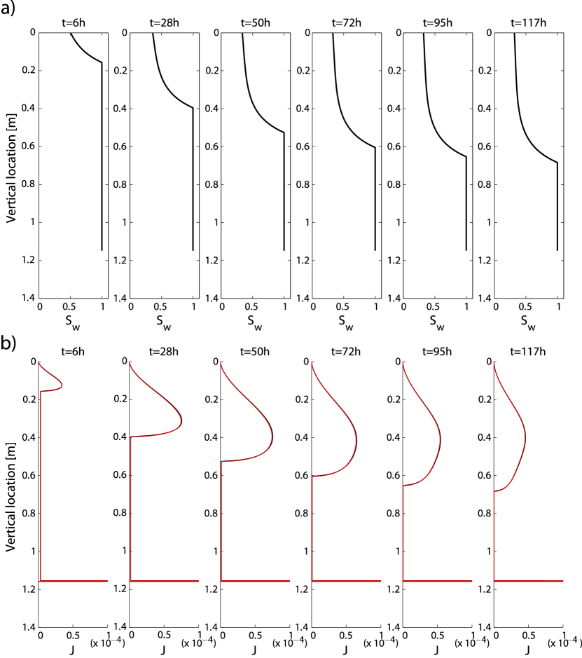
Figure 6: Snapshots of the water saturation profile (a) and total current density components $J_{cond}$ (black line) and $J_{conv}$ (red line, b) for six times between $t=6$ h and $t=117$ h. The electrical current density is expressed in A.m^-2. The snapshot corresponds to the simulation performed using the equation 28 for implementation of $C(S_{e})$ in the Poisson’s equation.

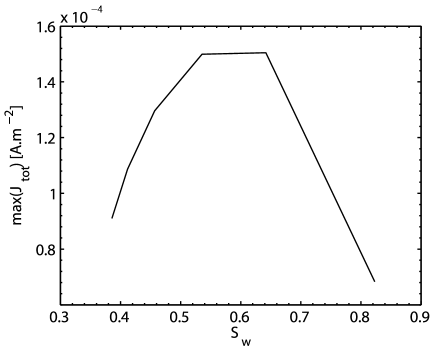
Figure 7: Maximum of the total current density $J$ (black line) inferred from curves in Figure 6 and corresponding water flow velocity (dashed black line).

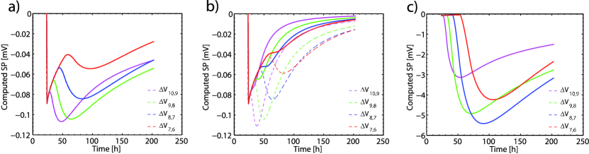
Figure 8: Computed SP (lines) using equations 26 (a), 27 (b) and 28 (c) with $n=1.45$, compared to computed SP with $n=2.5$ (dashed lines).

The SP were computed solving equations 1 and 10 for the three presented models (Figure 3). The computed SP using Guichet et al. (2003) and Revil et al. (2007) models are very small compared to the measurements (Figure 3a,b). A jump, corresponding to the drainage start, is observed in SP signals at the beginning of the simulation. Its magnitude is around 0.09 mV for tests performed using equations 26 and 27 and is the same for all dipoles (Figure 3d,e). In the case of Guichet et al. (2003) model (Figure 3d), the computed SP begin to decrease to reach a minimum value for dipoles (10,9) and (9,8) around -0.11 mV and then increase. This minimum is observed at the time when water saturation stops to decrease for all dipoles. In the case of Revil et al. (2007) model, the increasing of computed SP is monotonous during the simulation, from a value around -0.09 mV to almost 0 for all dipoles. It is obvious that these two models are not appropriate to explain the SP measurements both in terms of magnitude and behaviour.
Revil et al. (2007) used $L=$1 in their model, instead of $L=$0.5 as proposed by Mualem (1976) to hold as the best value for forty-five soils including sand. Consequently, the equation 27 was also implemented using $L=$0.5, which leads to a modified Revil et al. (2007) model. The results (Fig. 3e) are similar to those for $L=$1 in terms of amplitude, but show an increasing of SP signals without any step as it was observed before. The choice of $L$ is quite important because it’s involved in the global power law in eq. 27, and consequently influences the shape of the model (Allègre et al., 2010).
On the other hand, the model introduced for $C_{r}$ by equation 28 leads to good results in terms of computed SP. The measured SP signals are well reproduced, particularly at the beginning of the experiment between $t\simeq 20$ h and $t\simeq 100$ h. The computed SP corresponding to dipoles (10,9) to (7,6) decrease one after the other when water saturation (measured at the same level) begins to decrease (see Fig. 2b and 3c). Thus, the saturation front propagation is characterized by the time shift between SP decreasing starts. The computed SP using both equations 26 and 27 are up to one and a half order of magnitude smaller than those computed using expression 28 (Fig. 3).
For times over 100 hours, the residuals between measured and computed SP are larger. At this point of the experiment the water flow is very low, leading to very small variations of SP. This point is interpreted in Allègre et al. (2010), who precise that for such low water outflow (even not measurable), the SP variations are too weak to insure robust interpretation. Consequently, a better fit was expected at the beginning of the experiment (when the water flow is maximum), which is the case for three measurement dipoles. In addition, all the tests performed to ensure the quality of SP recordings and prevent the external sources of noise from disturbing the measurements, including a statistical study on uncertainties, can be found in Allègre et al. (2010) (Appendices A, B). Moreover, the fit and estimation of the set of parameters of eq. 28 would be improved if the SP measurements were inverted. Thus a joint inversion would give more informations on parameters sensitivities.
One can verify the assumption made by Allègre et al. (2010) to use eq. (12) to inferred SP coefficients from SP measurements. Thus, SP coefficients was computed using eq. (12), and compared to SP coefficients computed with eq. (28) averaged on 10 cm to be representative of the same investigated volume (Fig. 4). It is shown that SP coefficients using eqs (12) and (28) give very close results in terms of behaviour and magnitude. This example prove the validity of using eq. (12) to infer accurate values of $C$ even for non-steady conditions. One can consider that these values are apparent SP coefficients because the water saturation distribution is not perfectly homogeneous in 10 cm of sand, however they are still perfectly representative of true SP coefficients, at least for this kind of drainage experiment.
Furthermore, computed SP coefficients using different assumptions for $C_{r}$ (equations 26, 27 and 28) can be compared to measurements of $\Delta V$/ $\Delta P$ from Allègre et al. (2010) (Fig. 5). The fitted values of $\beta$, $\gamma$, and parameters of equations 26 and 27 are reported in the Table 3. It is clear on figure 5 that the two existing models for $C_{r}$ predict lower values of $C_{r}$ than measurements and fail to provide the correct behaviour of $C_{r}$. Moreover, the measured SP coefficients $\Delta V$/ $\Delta P$ are quite well reproduced in the case of using equation 28. It is important to notice that Allègre et al. (2010) inferred experimental SP coefficients using the equation 12 which is classically used for steady-state flows, neglecting electrokinetic sources coming from SP coefficient and electrical conductivity contrasts. Since no electrokinetic sources have been neglected in the present modelling, one can conclude that the non-monotonous behaviour combined to large values of $C_{r}$ observed previously are not artefacts and are not created by neglected contrasts of $C_{r}$ or $\sigma_{r}$ but has a physical origin. Therefore we show that the measurement of apparent $\Delta V/\Delta P$ for the dipoles can provide the streaming potential coefficient $C_{r}$ in these conditions. Nevertheless, a slight difference is observed between the maximum of computed and measured SP coefficients. These differences come from the use of the equation 12 to infer SP coefficients. Finally, these results confirm that a different maximum in $C_{r}$ for each dipole is necessary to provide accurate computed SP differences. We suggest that this observation has a physical meaning coming from the flow behaviour. Indeed, each dipole is not affected by the same hydrodynamic conditions, and particularly the same flow velocity, when water saturation (at its level) decreases.
An important point to discuss is the behaviour of the total current density. The figure 6 shows six snapshots of both water saturation and current density component $J_{cond}=-\sigma_{r}\boldsymbol{\nabla}V$ and $J_{conv}=\sigma_{r}C\boldsymbol{\nabla}P$ vertical profiles at six time during the simulation. The components $J_{cond}$ and $J_{conv}$ are computed a posteriori using finite differences. Even if SP sources are linked to $\boldsymbol{\nabla}\cdot$ J, as introduced by the conservation equation (eq. 9), we think that the vertical component of J is still relevant to describe the general behaviour of SP signals. This representation is usefull a posteriori to interpret the global SP variations, as it integrates all electrokinetic sources coming from SP coefficient or electrical conductivity contrasts (see eq. 10). The water saturation vertical profiles characterizes the propagation of saturation front during the drainage. In the saturated part of the column, $\theta=\theta_{s}$ thus $S_{w}=1$. In the unsaturated part, the saturation decreases from the top to the saturation front. The saturation value at the top of the system decreases during drainage from $S_{w}(z=0)=0.5$ at $t=6$ h to $S_{w}(z=0)=0.33$ at $t=50$ h and then stabilizes. For times greater than $t=50$ h, the water saturation is almost constant ($S_{w}\simeq 0.33$) for $0<z<40$ cm. Moreover, it is shown on figure 6b that the conduction ($J_{cond}$) and the convection ($J_{conv}$) component of the total current density $J$ are almost equal in absolute terms in the whole system during the entire experiment. The maximum difference observed between computed $J_{cond}$ and $J_{conv}$ does not exceed 2 per cent. This is a crucial point because the relation $J_{cond}=J_{conv}$ allows the use of equation 12 (i.e $C=\Delta V/\Delta P$) to deduce SP coefficient values from measurements. This is another confirmation that this approach can be used and gives accurate results for this kind of experimental conditions.
A large discontinuity is observed at the bottom of the column. This comes from the important contrast of electrical conductivity between the saturated medium and the water in the reservoir at the bottom of the column. Thus, the electrical conductivity changes from $\sigma_{sat}\simeq 0.002$ S.m^-1 to $\sigma_{w}=0.01$ S.m^-1 at this boundary. This is the only possible source of current since the SP coefficient is zero in water. Nevertheless, this contrast does not influence the SP measurements, since the measurement are located far from it and that the current density returns to a constant value in the centimetre above it. It was suggested by Linde et al. (2007) and Revil and Linde (comment submitted), that this contrast could be responsible for the behaviour of the measured SP. However, it is not the case for our experiment but may occur for measurements involving an electrode very close to this source. It should be then considered as an experimental artefact in this case.
The second point is that the maxima of $J_{cond}$ and $J_{conv}$ are not located at the higher gradient of water saturation (at the saturation front), corresponding to the higher contrast of electrical conductivity $\sigma_{r}$, but backward from this front. Its absolute value varies not linearly from $3\times$ 10^-5 A.m^-2 to $6.8\times$ 10^-5 A.m^-2 for 6 h $<t<$ 117 h (Figure 7). This suggests that the predominant contribution to the total electrical density comes from contrasts in SP coefficient which is larger for $S_{w}\simeq 0.8$ than for saturated conditions. This is obviously a consequence of the behaviour of $C_{r}$ as a function of water saturation. Thus, it seems that the electrokinetic response could be dominated by SP coefficient gradients and not by electrical conductivity gradients for such water flow.
This statement can be investigated using different parameters in the Archie’s law (eq. 29) to increase the influence of the electrical conductivity. Thus, the previous value of $n=1.45$ is replaced by a larger value as $n=2.5$. The influence of the saturation exponent $n$ depends on the considered model for the SP coefficient (Fig. 8a,b,c). Indeed, any change in $n$ does not influence the computed SP in the case of using equations 26 or 28 for calculation. On the contrary, the increasing of $n$ from $1.45$ to $2.5$ changes both the behaviour and magnitude of computed SP when the equation 27 is implemented (Fig. 8b). Thus, resulting SP exhibit larger values than the previous ones. This is explained by the increasing of the SP coefficient value implied by the increasing of $n$ (see eq. 27). It suggests that electrical conductivity contrasts are insignificant on the computed SP compared to other electrokinetic sources induced by SP coefficient contrasts.
One can conclude that a non-monotonous behaviour combined to large values of $C(S_{w})$ needs to be implemented in the Poisson’s equation to obtain computed SP close from the measured one. Nevertheless, the expression presented in this work is not sufficient and our approach does not deal with physical considerations. In future work, the water-flow conditions of the drainage experiment and especially the pressure dynamic and flow velocity could be involved in the observed SP coefficient behaviour.

6 Conclusions

We presented in this work the first modelling of both Richards and Poisson’s equations for unsaturated conditions using 1D finite element method. Several simulations have been performed using three different hypotheses on the SP coefficient $C_{r}$ to deduce SP differences which have been compared to observations from Allègre et al. (2010). The two existing models from Guichet et al. (2003) and Revil et al. (2007) were not able to predict SP differences consistent with the measurements of Allègre et al. (2010), although no electrical current sources have been neglected. We proved with this modelling approach that a non-monotonous expression for $C(S_{e})$ is necessary to correctly reproduced these measurements. We also demonstrated the consistency of our SP coefficient dataset verifying the equality $J_{cond}=J_{conv}$, and consequently the possibility to use the apparent $\Delta$V / $\Delta$P measurements to infer correct $C$ values for this kind of drainage experiment. This conclusion has to be verified for other flow conditions, for example steady-state unsaturated flow conditions with various flow velocities using different sands.
Finally, a joint inversion approach of hydrodynamics and electrical potential, which could improve the modelling results of SP, is undergoing. This approach will help to insure the robustness of our model for long times and will define precisely the sensitivities of inverted model parameters.
For field applications, even if a good correlation can be observed between SP response and precipitation occurrence (Thony et al., 1997; Doussan et al., 2002), it seems that a linear relationship between water flux and electrical potential gradient would be difficult to establish. Indeed, non-linear effects coming from the behaviour of the SP coefficient for unsaturated conditions, show that this relationship is probably more complex. Moreover, some acquisition issues and changing soil conditions during long experiments make SP difficult to interpret (Doussan et al., 2002). However, shorter artificial infiltration experiments using SP monitoring could still be possible at the field scale. SP could be modelled with our new model of relative SP coefficient taking into account for infiltration and/or evaporation with time-varying upper boundary conditions. These experiments could be very useful to infer some hydrodynamic parameters of soils, such as hydraulic conductivity, and give a way to measure ground water flux in the vadose zone.

7 Acknowledgments

This work was supported by the French National Scientific Centre (CNRS), by ANR-TRANSEK, and by REALISE, the Alsace Region Research Network in Environmental Sciences in Engineering and the Alsace Region.

Table 1: Parameters used to perform the Darcy’s experiment simulation, deduced from Allègre et al. (2010).

$\sigma_{w}$ [S.m-1]	$C_{sat}$ [V.Pa-1]	$h_{0}$ [cm H2O]	$h_{l}$ [cm H2O]
103.2$\times$10-4	-1.6$\times$10-6	20	60

Table 2: Hydrodynamic parameters values used to solve the Richards equation for unsaturated conditions. The parameter $K_{s}^{meas}$ is the measured permeability of the sand. These two values of permeability lead to the same results for pressure and water-content behaviours.

$K_{s}$ (x$10^{-5}$) [m.s-1]	$K_{s}^{meas}$ (x$10^{-5}$) [m.s-1]	$h_{a}$ [m]	$\lambda$	$\theta_{r}$ [-]	$\theta_{s},\phi$ [-]	${S_{w}}^{r}$ [-]
1.65	17.2	0.4	3.88	0.11	0.36	0.305

Table 3: Parameters needed to implement equations 27, 28 and 29 in the Poisson’s equation. The four values given for $\beta$ corresponds to the dipoles from (10,9) to (7,6). The $n$ value was measured in (Allègre et al., 2010).

$C_{sat}$ [V.Pa-1]	$\sigma_{w}$ [S.m-1]	$n$ (Archie exponent)	$\beta$	$\gamma$
-1.6$\times$10-6	103.2$\times$10-4	1.45	32,52,72,92	0.4

References

- Allègre et al. (2010) Allègre, V., Jouniaux, L., Lehmann, F., & Sailhac, P., 2010. Streaming potential dependence on water-content in fontainebleau sand, Geophys. J. Int., 182, 1248–1266.
- Archie (1942) Archie, G. E., 1942. The electrical resistivity log as an aid in determining some reservoir characteristics, Trans. Am. Inst. Min. Metall. Pet. Eng., pp. 146–154.
- Bordes et al. (2006) Bordes, C., Jouniaux, L., Dietrich, M., Pozzi, J.-P., & Garambois, S., 2006. First laboratory measurements of seismo-magnetic conversions in fluid-filled fontainebleau sand, Geophys. Res. Lett., 33, L01302.
- Bordes et al. (2008) Bordes, C., Jouniaux, L., Garambois, S., Dietrich, M., Pozzi, J.-P., & Gaffet, S., 2008. Evidence of the theoretically predicted seismo-magnetic conversion, Geophys. J. Int., 174, 489–504.
- Brooks & Corey (1964) Brooks, R. J. & Corey, A. T., 1964. Hydraulic properties of porous media, Hydrol. Pap., 3, 318–333.
- Darnet et al. (2003) Darnet, M., Marquis, G., & Sailhac, P., 2003. Estimating aquifer hydraulic properties from the inversion of surface streaming potential (sp) anomalies, Geophys. Res. Lett., 1679(30).
- Darnet et al. (2006) Darnet, M., G.Marquis, & Sailhac, P., 2006. Hydraulic stimulation of geothermal reservoirs:fluid flow, electric potential and microseismicity relationships, Geophys. J. Int., 166, 438–444.
- Davis et al. (1978) Davis, J. A., James, R. O., & Leckie, J., 1978. Surface ionization and complexation at the oxide/water interface, Journal of Colloid and Interface Science, 63, 480–499.
- Doussan & Ruy (2009) Doussan, C. & Ruy, S., 2009. Prediction of unsaturated soil hydraulic conductivity with electrical conductivity, Water Resources Res., 45, W10408.
- Doussan et al. (2002) Doussan, C., Jouniaux, L., & Thony, J.-L., 2002. Variations of self-potential and unsaturated flow with time in sandy loam and clay loam soils, Journal of Hydrology, 267, 173–185.
- Dupuis et al. (2007) Dupuis, J. C., Butler, K. E., & Kepic, A. W., 2007. Seismoelectric imaging of the vadose zone of a sand aquifer, Geophysics, 72, A81–A85.
- Fenoglio et al. (1995) Fenoglio, M., Johnston, M., & Byerlee, J., 1995. Magnetic and electric fields associated with changes in high pore pressure in fault zones; application to the loma prieta ulf emissions, J. Geophys. Res., 100, 12951–12958.
- Finizola et al. (2002) Finizola, A., Sortino, F., Lenat, J.-F., & Valenza, M., 2002. Fluid circulation at stromboli volcano (aeolian islands, italy) from self potential and co2 surveys, J. Volc. Geotherm. Res., (116), 1–18.
- Finizola et al. (2004) Finizola, A., Lenat, J.-F., Macedo, O., Ramos, D., Thouret, J.-C., & Sortino, F., 2004. Fluid circulation and structural discontinuities inside misti volcano (peru) inferred from sel-potential measurements, J. Volc. Geotherm. Res., 135(4), 343–360.
- Gardner (1958) Gardner, W. R., 1958. Some steady state solutions of the unsaturated moisture flow equation with application to evaporation from a water table, Soil Sciences, 85, 228–232.
- Gibert & Pessel (2001) Gibert, D. & Pessel, M., 2001. Identification of sources of potential fields with the continuous wavelet transform: application to self-potential profiles, Geophys. Res. Lett., 28, 1863–1866.
- Glover & Walker (2009) Glover, P. W. J. & Walker, E., 2009. Grain-size to effective pore-size transformation derived from electrokinetic theory, Geophysics, 74, E17–E29.
- Glover et al. (2006) Glover, P. W. J., Zadjali, I. I., & Frew, K. A., 2006. Permeability prediction from micp and nmr data using an electrokinetic approach, Geophysics, 71, F49–F60.
- Guichet et al. (2003) Guichet, X., Jouniaux, L., & Pozzi, J.-P., 2003. Streaming potential of a sand column in partial saturation conditions, J. Geophys. Res., 108(B3), 2141.
- Guichet et al. (2006) Guichet, X., Jouniaux, L., & Catel, N., 2006. Modification of streaming potential by precipitation of calcite in a sand-water system: laboratory measurements in the ph range from 4 to 12, Geophys. J. Int., 166, 445–460.
- Hayek et al. (2008) Hayek, M., Lehmann, F., & Ackerer, P., 2008. Adaptative multi-scale parametrization for one-dimensional flow in unsaturated porous media, Adv. Water Resour., 31, 28–43.
- Henry et al. (2003) Henry, P., Jouniaux, L., Screaton, E. J., S.Hunze, & Saffer, D. M., 2003. Anisotropy of electrical conductivity record of initial strain at the toe of the Nankai accretionary wedge, J. Geophys. Res., 108, 2407.
- Ishido & Mizutani (1981) Ishido, T. & Mizutani, H., 1981. Experimental and theoretical basis of electrokinetic phenomena in rock water systems and its applications to geophysics, J. Geophys. Res., 86, 1763–1775.
- Jaafar et al. (2009) Jaafar, M. Z., Vinogradov, J., & Jackson, M. D., 2009. Measurement of streaming potential coupling coefficient in sandstones saturated with high salinity nacl brine, Geophys. Res. Lett., 36, L21306.
- Jackson (2010) Jackson, M. D., 2010. Multiphase electrokinetic coupling: Insights into the impact of fluid and charge distribution at the pore scale from a bundle of capillary tubes model, J. Geophys. Res., 115, B07206.
- Jouniaux et al. (1994) Jouniaux, L., Lallemant, S., & Pozzi, J., 1994. Changes in the permeability, streaming potential and resistivity of a claystone from the nankai prism under stress, Geophys. Res. Lett., 21, 149–152.
- Jouniaux et al. (2006) Jouniaux, L., Zamora, M., & Reuschlé, T., 2006. Electrical conductivity evolution of non-saturated carbonate rocks during deformation up to failure, Geophys. J. Int., 167, 1017–1026.
- Jouniaux et al. (2009) Jouniaux, L., Maineult, A., Naudet, V., Pessel, M., & Sailhac, P., 2009. Review of self-potential methods in hydrogeophysics, C. R. Geoscience, 341, 928–936.
- Lehmann & Ackerer (1998) Lehmann, F. & Ackerer, P., 1998. Comparison of iterative methods for improved solutions of the fluid flow equation inpartially saturated porous media, Transport in Porous media, 31, 275–292.
- Linde et al. (2007) Linde, N., Jougnot, D., Revil, A., Matthai, S. K., Renard, D., & Doussan, C., 2007. Streaming current generation in two-phase flow conditions, Geophys. Res. Lett., 34, LO3306.
- Lorne et al. (1999) Lorne, B., Perrier, F., & Avouac, J.-P., 1999. Streaming potential measurements. 1. properties of the electrical double layer from crushed rock samples, J. Geophys. Res., 104(B8), 17.857–17.877.
- Maineult et al. (2006a) Maineult, A., Bernabé, Y., & Ackerer, P., 2006a. Detection of advected, recating redox fronts from self-potential measurements, J. Contaminant Hydrology, (86), 32–52.
- Maineult et al. (2006b) Maineult, A., Jouniaux, L., & Bernabé, Y., 2006b. Influence of the mineralogical composition on the self-potential response to advection of kcl concentration fronts through sand, Geophys. Res. Lett., (33), L24311.
- Maineult et al. (2008) Maineult, A., Strobach, E., & Renner, J., 2008. Self-potential signals induced by periodic pumping test, J. Geophys. Res., 113, B01203.
- Mauri et al. (2010) Mauri, G., Williams-Jones, G., & Saracco, G., 2010. Depth determinations of shallow hydrothermal system by self-potential and multi-scale wavelet tomography, J. Volc. Geotherm. Res., 191, 233–244.
- Mualem (1976) Mualem, Y., 1976. A new model for predicting the hydraulic conductivity of unsaturated porous media, Water Resour. Res., 12, 513–522.
- Naudet et al. (2003) Naudet, V., Revil, A., Bottero, J.-Y., & Bégassat, P., 2003. Relationship between self-potential (sp) signals and redox conditions in contaminated groundwater, Geophys. Res. Lett., 30(21).
- Onizawa et al. (2009) Onizawa, S., Matsushima, N., Ishido, T., Hase, H., Takakura, S., & Nishi, Y., 2009. Self-potential distribution on active volcano controlled by three-dimensional resistivity structure in izu-oshima, japan, Geophys. J. Int., 178, 1164–1181.
- Onsager (1931) Onsager, L., 1931. Reciprocical relation in irreversible processes: I, Phys. Rev, 37.
- Overbeek (1952) Overbeek, J. T. G., 1952. Electrochemistry of the double layer., Colloid Science, Irreversible Systems, edited by H. R. Kruyt, Elsevier, 1, 115–193.
- Perrier & Morat (2000) Perrier, F. & Morat, P., 2000. Characterization of electrical daily variations induced by capillary flow in the non-saturated zone, Pure and Appl. Geophys, 157, 785–810.
- Pinder & Gray (1977) Pinder, G. F. & Gray, W. G., 1977. Finite element simulation in surface and subsurface hydrology, New York: Academic Press.
- Pozzi & Jouniaux (1994) Pozzi, J.-P. & Jouniaux, L., 1994. Electrical effects of fluid circulation in sediments and seismic prediction, C.R. Acad. Sci. Paris, serie II, 318(1), 73–77.
- Press et al. (1992) Press, W. H., Teukolsky, S., Vetterling, W. T., & Flannery, B. P., 1992. Numerical recipes in fortran, the art of scientific computing, Second edition, Cambridge University Press, Cambridge.
- Pride (1994) Pride, S., 1994. Governing equations for the coupled electromagnetics and acoustics of porous media, Physical Review B, 50, 15678–15695.
- Pride & Morgan (1991) Pride, S. & Morgan, F. D., 1991. Electrokinetic dissipation induced by seismic waves, Geophysics, 56(7), 914–925.
- Revil et al. (2007) Revil, A., Linde, N., Cerepi, A., Jougnot, D., Matthai, S., & Finsterle, S., 2007. Electrokinetic coupling in unsaturated porous media, Journal of Colloid and Interface Science, 313, 315–327.
- Richards (1931) Richards, L. A., 1931. Capillary conduction of liquids through porous medium, Physics, 1, 318–333.
- Sailhac et al. (2004) Sailhac, P., Darnet, M., & Marquis, G., 2004. Electrical streaming potential measured at the ground surface: forward modeling and inversion issues for monitoring infiltration and characterizing the vadose zone, Vadose Zone J., (3), 1200–1206.
- Saracco et al. (2004) Saracco, G., Labazuy, P., & Moreau, F., 2004. Localization of self-potential sources in volcano-electric effect with complex continuous wavelet transform and electrical tomography methods for an active volcano, Geophys. Res. Lett., (31), L12610.
- Saunders et al. (2008) Saunders, J. H., Jackson, M. D., & Pain, C. C., 2008. Fluid flow monitoring in oilfields using downhole measurements of electrokinetic potential, Geophysics, 73, E165–E180.
- Sheffer & Oldenburg (2007) Sheffer, M. R. & Oldenburg, D. W., 2007. Three-dimensional modelling of streaming potential, Geophys. J. Int., 169, 839–848.
- Thony et al. (1997) Thony, J. L., Morat, P., Vachaud, G., & Mouël, J. L., 1997. Field characterization of the relationship between electrical potential gradients and soil water flux, CR Acad. Sci. Paris, Earth Planetary Sci., 325, 317–321.
- Tosha et al. (2003) Tosha, T., Matsushima, N., & Ishido, T., 2003. Zeta potential measured for an intact granite sample at temperatures to 200c, Geophys. Res. Lett., 30(6).
- van Genuchten (1980) van Genuchten, M. T., 1980. A closed-form equation for predicting the hydraulic conductivity of unsaturated soil, Soil Sci. Soc. Am. J., 44, 892–898.
- Vinogradov et al. (2010) Vinogradov, J., Jaafar, M., & Jackson, M. D., 2010. Measurement of streaming potential coupling coefficient in sandstones saturated with natural and artificial brines at high salinity, J. Geophys. Res., 115, B12204.