Subarcsecond resolution observations of warm water towards three deeply embedded low-mass protostars

Abstract

Context. Water is present during all stages of star formation: as ice in the cold outer parts of protostellar envelopes and dense inner regions of circumstellar disks, and as gas in the envelopes close to the protostars, in the upper layers of circumstellar disks and in regions of powerful outflows and shocks. Because of its key importance in the understanding of its origin in our own solarsystem, following the evolution of water all the way to the planet-forming disk is a fundamental task in research in star formation and astrochemistry.

Aims. In this paper we probe the mechanism regulating the warm gas-phase water abundance in the innermost hundred AU of deeply embedded (Class 0) low-mass protostars, and investigate its chemical relationship to other molecular species during these stages.

Methods. Millimeter wavelength thermal emission from the para-H${}_{2}^{18}$O $3_{1,3}-2_{2,0}$ ($E_{\mathrm{u}}$=203.7 K) line is imaged at high angular resolution (0$\aas@@fstack{\prime\prime}$75; 190 AU) with the IRAM Plateau de Bure Interferometer towards the deeply embedded low-mass protostars NGC 1333-IRAS2A and NGC 1333-IRAS4A.

Results. Compact H${}_{2}^{18}$O emission is detected towards IRAS2A and one of the components in the IRAS4A binary; in addition CH₃OCH₃, C₂H₅CN, and SO₂ are detected. Extended water emission is seen towards IRAS2A, possibly associated with the outflow.

Conclusions. The results complement a previous detection of the same transition towards NGC 1333-IRAS4B. The detections in all systems suggests that the presence of water on $\lesssim$ 100 AU scales is a common phenomenon in embedded protostars and that the non-detections of hot water with Spitzer towards the two systems studied in this paper are likely due to geometry and high extinction at mid-infrared wavelengths. We present a scenario in which the origin of the emission from warm water is in a flattened disk-like structure dominated by inward motions rather than rotation. The gas-phase water abundance varies between the sources, but is generally much lower than a canonical abundance of 10^-4, suggesting that most water (>96%) is frozen out on dust grains at these scales. The derived abundances of CH₃OCH₃ and SO₂ relative to H${}_{2}^{18}$O are comparable for all sources pointing towards similar chemical processes at work. In contrast, the C₂H₅CN abundance relative to H${}_{2}^{18}$O is significantly lower in IRAS2A, which could be due to different chemistry in the sources.

1 Introduction

Water is a key molecule in regions of star formation. In cold outer regions of protostellar envelopes and dense mid-planes of circumstellar disks, it is the most abundant molecule in the ices on dust grains (e.g. Gibb et al. 2004; Boogert et al. 2008). In regions of increased temperatures (e.g., due to protostellar heating or active shocks) it desorbs and becomes an important coolant for gas (Ceccarelli et al. 1996; Neufeld & Kaufman 1993). As one of the major oxygen reservoirs it also influences the oxygen based chemistry (e.g. van Dishoeck & Blake 1998). This paper presents high-angular resolution observations (0$\aas@@fstack{\prime\prime}$75) at 203.4 GHz of the H${}_{2}^{18}$O isotopologue towards two deeply embedded (Class 0) low-mass protostars using the Institute de Radioastronomie Millimétrique (IRAM) Plateau de Bure Interferometer (PdBI), one of the few water lines that can be routinely observed from Earth. The aim of the observations is to determine the origin of water emission lines in the inner 100 AU of these protostars.

The young, dust- and gas-enshrouded protostars provide an important laboratory for studies of the star formation process. On the one hand, they provide the link between the prestellar cores and the young stellar objects (YSOs) and on the other hand it is likely that during these stages the initial conditions for the later astrochemical evolution of the protostellar envelopes and disks are established (e.g., Visser et al. 2009). In the earliest stages most of the gas and dust is present on large scales in the protostellar envelopes where the temperatures are low (10–20 K) and most molecules, including water, are locked up as ice on grains. Nevertheless, space-based observations from ISO, SWAS, Odin, Spitzer and Herschel show that significant amounts of gas-phase water are present towards even deeply embedded protostars, pointing to significant heating and processing of water-ice covered grains (Nisini et al. 1999; Ceccarelli et al. 1999; Maret et al. 2002; Bergin et al. 2003; Franklin et al. 2008; Watson et al. 2007; van Dishoeck et al. 2011; Kristensen et al. 2010).

Exactly which mechanism regulates where and how the heating and evaporation of the water ice takes place is still debated. Proposed locations and mechanisms include the innermost envelope, heated to temperatures larger than 100 K by the radiation from the central protostar on scales $\lesssim$100 AU (Ceccarelli et al. 1998; Maret et al. 2002), in shocks of the protostellar outflow (Nisini et al. 1999), or in the disk – heated either by shocks related to ongoing accretion onto the circumstellar disks or in their surface layers heated by the protostar (Watson et al. 2007; Jørgensen & van Dishoeck 2010a).

Recently, Watson et al. (2007) observed 30 Class 0 protostars, including the sources in this paper, with the infrared spectrograph (IRS) on board Spitzer. The protostar NGC 1333-IRAS4B (IRAS4B) showed a wealth of highly excited H₂O lines, and was the only source in the sample in which the water lines were detected. By modeling the spectra they concluded that because of the high inferred density and temperature of the water, it originates in the vicinity of the protostar, likely accretion shocks in the circumstellar disk. However, the Spitzer data, and similar observations from space, lack the spatial and spectral resolution to unambiguously associate the emission with the components in the protostellar systems – and can for the shorter wavelengths also be hampered by extinction by the dust in the protostellar envelopes and disks. Herczeg et al. (2011) analyzed the emission from warm water lines in maps toward IRAS4B obtained with the PACS instrument on the Herschel Space Observatory. The maps show that the bulk of the warm water emission has its origin in a outflow-driven shock offset by about 5″ (1200 AU) from the central protostar. An excitation analysis of the emission furthermore shows that the temperature in the shocked region is about 1500 K, which can simultaneously explain both the far-IR (Herschel) and mid-IR (Spitzer) water lines.

Higher angular and spectral resolution is possible through interferometric observations of H${}_{2}^{18}$O which has a few transitions that can be imaged from the ground (e.g. Jacq et al. 1988; Gensheimer et al. 1996; van der Tak et al. 2006). Jørgensen & van Dishoeck (2010a) report observations of IRAS4B with the PdBI. They detect the H${}_{2}^{18}$O $3_{1,3}-2_{2,0}$ line at 203.4 GHz, and also resolve a tentative velocity gradient in the very narrow line ($\sim$2 km s^-1 width at zero intensity), indicating an origin of the H${}_{2}^{18}$O emission in a rotational structure. The H₂O column density is around 25 times higher than previously estimated from mid-IR observations by Watson et al. (2007), on similar size scales (inner 25 AU of the protostar).

This study presents similar high angular resolution H${}_{2}^{18}$O millimeter wavelength observations for the sources NGC 1333-IRAS2A (IRAS2A) and NGC 1333-IRAS4A (IRAS4A), which are compared to IRAS4B. The three sources are all deeply embedded Class 0 protostars in the nearby NGC 1333 region of the Perseus molecular cloud identified through early infrared and (sub)millimeter wavelength observations (e.g., Jennings et al. 1987; Sandell et al. 1991). All sources were mapped by Spitzer (Jørgensen et al. 2006; Gutermuth et al. 2008), and were part of the high resolution ($\sim$1″) PROSAC survey of Class 0/I sources using the Submillimeter Array (SMA; Jørgensen et al. 2007, 2009). Their similar luminosities (20, 5.8, 3.8 $L_{\rm\sun}$ for IRAS2A, IRAS4A and IRAS4B, respectively) and envelope masses (1.0, 4.5², 2.9 $M_{\rm\sun}$, respectively) from those surveys, and thus presumably also similar evolutionary stages, make them ideal for studying and comparing deeply embedded young stellar objects in the same environment.

IRAS4A is a binary system with a 1$\aas@@fstack{\prime\prime}$8 separation (Looney et al. 2000; Reipurth et al. 2002; Girart et al. 2006), associated with a larger scale jet and outflow (e.g. Blake et al. 1995; Jørgensen et al. 2007). The jet axis has been deduced from water maser observations associated to IRAS4A-NW to $2\degr$ in the plane of the sky and at a position angle (PA) of $-50\degr$ (north through east, Marvel et al. 2008; Desmurs et al. 2006), almost perpendicular to the CO outflow axis (PA$=0\degr-45\degr$; Blake et al. 1995; Jørgensen et al. 2007). The mass of the NW source is estimated from modeling to 0.08 $M_{\rm\sun}$ (Choi et al. 2010), no estimate of the mass of the SE source exists. The envelope is dominated by inward motion, as evident from the inverse P-Cygni profiles in the spectra and modeling of gas kinematics (Di Francesco et al. 2001; Attard et al. 2009; Kristensen et al. 2010).

The other source, IRAS2A, shows two bipolar outflows, one shell-like directed N-S (PA$\approx+25\degr$, Jørgensen et al. 2007) and the other a jet-like directed E-W (PA$\approx+105\degr$, Liseau et al. 1988; Sandell et al. 1994; Jørgensen et al. 2004). Water maser emission has been detected towards IRAS2A, partly associated with the northern redshifted outflow (Furuya et al. 2003). One proposed solution to the presence of a quadrupolar outflow is that IRAS2A is a binary system with 0$\aas@@fstack{\prime\prime}$3 (75 AU) separation (Jørgensen et al. 2004).

The paper is laid out as follows. Sect. 2 presents the interferometric observations of the three Class 0 sources that the paper is based upon. Sect. 3 presents the results from the analysis of the spectra and maps. Sect. 4 discusses the detection of water, and the column density estimates. Sect. 5 presents a summary of the important conclusions and suggests possible future work.

2 Observations

Three low-mass protostars, IRAS2A, IRAS4A-SE and -NW in the embedded cluster NGC 1333 in the Perseus molecular cloud were observed using the PdBI. IRAS2A and IRAS4A were observed in two configurations each: the B configuration on 6, 15 and 17 March 2010 and the C configuration on 9 December 2009. The sources were observed in track-sharing mode for a total of 12 hours in B configuration and about 8 hours in C configuration. Combining the observations in the different configurations, the data cover baselines from 15.4 to 452 m (10.5 to 307 k$\lambda$). The receivers were tuned to the para-H${}_{2}^{18}$O $3_{1,3}-2_{2,0}$ transition at 203.40752 GHz (1.47 mm) and the correlators were set up with one unit with a bandwidth of 40 MHz (53 km s^-1) centered on this frequency providing a spectral resolution on 460 channels of 0.087 MHz (0.115 km s^-1) width.

The data were calibrated and imaged using the CLIC and MAPPING packages, which are parts of the IRAM GILDAS software. The general calibration procedure was followed: regular observations of the nearby, strong quasar 0333+3221 were used to calibrate the complex gains and bandpass, while MWC349, 0333+3221 and 3C84 were observed to calibrate the absolute flux scale. Integrations with significantly deviating amplitudes/phases were flagged and the continuum was subtracted before Fourier transformation of the data. The resulting beam sizes using natural weighting, along with other data, are given in Table 1. The field of view is 25″(HPBW) at 1.45 mm and the continuum sensitivity is limited by the dynamical range of the interferometer while the line data RMS is given in Table 1. The uncertainty in fluxes is dominated by the flux calibration error, typically 20%.

Table 1: Observation parameters.

Source	Beam	PA	RMS
IRAS2A	0$\aas@@fstack{\prime\prime}$87 x 0$\aas@@fstack{\prime\prime}$72	63.5°	16.1
IRAS4A(-SE/NW)	0$\aas@@fstack{\prime\prime}$86 x 0$\aas@@fstack{\prime\prime}$70	63.4°	16.5

3 Results

Continuum emission from the targeted sources (IRAS2A and the IRAS4A-NW and IRAS4A-SE binary) was detected at levels expected from previous high resolution millimeter wavelength continuum observations: parameters from elliptical Gaussian fits to the continuum emission for the sources are given in Table 2. The continuum emission towards the sources is resolved and the fluxes concur with the results of Jørgensen et al. (2007), assuming a power-law spectrum ($F_{\nu}$ $\propto$ $\nu^{\alpha}$) with $\alpha$$\sim$2.3–2.7, expected for thermal dust continuum emission.

Table 2: Parameters for the sources from elliptical Gaussian fits to their continuum emission. Errors given are the statistical errors from the fitting routine.

	IRAS2A	IRAS4A-NW	IRAS4A-SE
Flux ($\pm$)	$0.24$ (0.002) Jy	$0.88$ (0.025) Jy	$1.46$ (0.021) Jy
R.A ($\pm$)	03:28:55.57 (0$\aas@@fstack{\prime\prime}$004)	03:29:10.44 (0$\aas@@fstack{\prime\prime}$02)	03:29:10.53 (0$\aas@@fstack{\prime\prime}$005)
Dec ($\pm$)	31:14:37.03 (0$\aas@@fstack{\prime\prime}$004)	31:13:32.16 (0$\aas@@fstack{\prime\prime}$02)	31:13:30.92 (0$\aas@@fstack{\prime\prime}$006)
Extent	$1\aas@@fstack{\prime\prime}1\times 1\aas@@fstack{\prime\prime}0\leavevmode\nobreak\ (23^{\circ})$	$2\aas@@fstack{\prime\prime}0\times 1\aas@@fstack{\prime\prime}2\leavevmode\nobreak\ (-53^{\circ})$	$1\aas@@fstack{\prime\prime}4\times 1\aas@@fstack{\prime\prime}0\leavevmode\nobreak\ (50^{\circ})$

Fig. 1 shows the spectrum towards the continuum peak of these sources, as well as IRAS4B (Jørgensen & van Dishoeck 2010a). A number of lines are detected towards IRAS2A and one component in the IRAS4A protobinary system, IRAS4A-NW. IRAS4A-SE in contrast does not show any emission lines in the high-resolution spectra, and it is therefore only listed in the table showing the characteristics of the continuum emission.

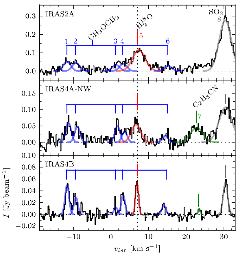
Figure 1: Spectra extracted in a pixel towards the continuum peak positions for IRAS2A, IRAS4A-NW and IRAS4B. The identified lines are marked, including the targeted H${}_{2}^{18}$O $3_{1,3}-2_{2,0}$ line. Parameters from the fits are tabulated in Table 6.2. The numbers above the lines and the colors correspond to the numbers (emission lines) and colors in Fig. 3, Table 3, Table 5 and Table 6.2. The spectra have been binned to a width of 0.23 km s^-1 (i.e., 2 channels per bin), and Gaussian profiles have been fitted to the identified lines. The systemic velocity of the H${}_{2}^{18}$O line is marked by the vertical dotted line at $v_{\mathrm{lsr}}=7.0$ km s^-1. Note the difference in scale of the y-axis for the spectra.

The Jet Propulsion Laboratory (JPL, Pickett et al. 1998) and the Cologne Database for Molecular Spectroscopy (CDMS, Müller et al. 2001) databases were queried through the Splatalogue interface to identify the lines. The line widths and strengths vary between the sources and because of the broader line widths some blending between the different CH₃OCH₃ lines occurs in both IRAS2A and IRAS4A-NW. As seen in Fig. 1, several lines are detected: the target water line, SO₂ and several lines of CH₃OCH₃. C₂H₅CN is seen in IRAS 4A-NW and IRAS4B, but not in IRAS2A.

Particular interesting for this study is the assignment of the H${}_{2}^{18}$O $3_{1,3}-2_{2,0}$ transition ($E_{\mathrm{u}}$=203.7 K). No other lines fall within $\pm$1 km s^-1 of the H${}_{2}^{18}$O $3_{1,3}-2_{2,0}$ line listed in the spectral line catalogs. The lines that fall close ($\pm$1-2 km s^-1) are ¹³CH₂CHCN, ¹³CH₃CH₂CN and (CH₃)₂CO. Both the ¹³CH₂CHCN and ¹³CH₃CH₂CN isotopologues have other transitions which would have been detected, whereas a possible transition of (CH₃)₂CO has a too low intrinsic line strength to be plausible.

In Fig. 2 the integrated intensity (zeroth order moment) and velocity (first order moment) maps for the H${}_{2}^{18}$O transition are shown for the observed sources. For IRAS2A the calculations were made over the velocity interval from 4.4 to 11.4 km s^-1 and for IRAS4A-NW from 4.7 to 9.6 km s^-1. The integrated intensity maps for IRAS2A show some extended emission, whereas for IRAS4A-NW the emission is compact around the continuum peak with a slight elongation in the north-south direction. The velocity maps for both IRAS2A and IRAS4A (right hand panels in Fig. 2) show no obvious spatial gradients in velocity, neither on source nor along the outflow in IRAS2A.

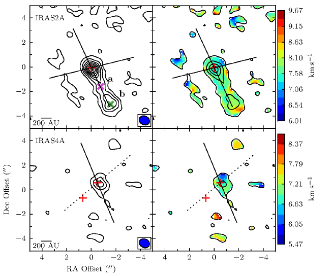
Figure 2: Integrated intensity (left) and velocity (right) maps for the H${}_{2}^{18}$O $3_{1,3}-2_{2,0}$ line in IRAS2A (from 4.4 to 11.4 km s^-1) and IRAS4A (from 4.7 to 9.6 km s^-1). Contours show integrated intensity and are in steps of 4$\sigma$ for the intensity map, 8$\sigma$ for the velocity map, and start at 3$\sigma$. The position of the continuum emission is marked by a red plus sign, an outflow by the solid line and maser emission by the dashed line. Positions where spectra have been extracted in IRAS2A along the outflow are marked with letters a and b and crosses with magenta and green colors in the integrated intensity map.

For estimates of the physical conditions in the gas, circular Gaussian profiles were fitted to the emission of each line in the $(u,v)$-plane. The fits were performed to the line intensities typically integrated over the line widths ($v_{\rm lsr}\pm$FWHM) and are given in Table 3. Table 5 lists the molecular parameters adopted in this paper of the target line H${}_{2}^{18}$O $3_{1,3}-2_{2,0}$, and other detected lines, while Table 6.2 lists the position, FWHM and integration interval for the different lines.

Table 3: Parameters for the lines detected in the sources from circular Gaussian fits to the integrated line maps. Molecule specific data are tabulated in Table 5 and the integration interval (in km s^-1) in Table 6.2 in the appendix.

				IRAS2A				IRAS4A-NW
No.	Molecule	Transition	Flux	Offset	Size		Flux	Offset	Size
			(Jy km s-1)	(″)	(″)		(Jy km s-1)	(″)	(″)
1	CH3OCH3	33,0 – 22,1 EE	$0.47$	$-0.02;-0.002$	$0.70\pm 0.09$		$0.44$	$-0.21;-0.04$	$0.70\pm 0.09$
2	CH3OCH3	33,0 – 22,1 AA	$-$	$-;-$	$-$		$-$	$-;-$	$-$
3	CH3OCH3	33,0 – 22,1 AE	$0.81$	$-0.16;-0.32$	$1.45\pm 0.10$		$0.26$	$-0.14;-0.03$	$0.57\pm 0.12$
4	CH3OCH3	33,1 – 22,1 EE	$-$	$-;-$	$-$		$-$	$-;-$	$-$
5	H${}_{2}^{18}$O	31,3 – 22,0	$0.98$	$-0.07;-0.12$	$0.83\pm 0.05$		$0.27$	$-0.18;-0.07$	$0.61\pm 0.12$
6	CH3OCH3	33,1 – 22,1 EA	$0.30$	$-0.35;-0.52$	$1.23\pm 0.22$		$0.06$	$-0.25;-0.10$	$0.44\pm 0.26$
7	C2H5CN	232,22 – 222,21	$<0.04$	$-;-$	$-$		$0.27$	$-0.20;-0.05$	$0.37\pm 0.11$
8	SO2	120,12 – 111,11	$2.73$	$-0.07;+0.003$	$1.00\pm 0.02$		$1.22$	$-0.22;-0.01$	$0.88\pm 0.05$

4 Analysis and discussion

The detected water lines provide important constraints on the physical and chemical structure of the deeply embedded low-mass protostars, which we discuss in this section. The first part of the discussion (Sect. 4.1–4.3) focuses on the detection of warm water on scales comparable to the protostellar disk and the extended emission found in the outflow towards IRAS2A. The implications for the geometry and dynamics are also discussed. The second part (Sect. 4.4-4.6) discusses excitation conditions in the water emitting gas and the column densities and relative abundances of water and other species detected on small scales.

4.1 Water on small scales

The key result from the presented observations is the detection of compact H${}_{2}^{18}$O in IRAS2A and IRAS4A-NW, adding to the discovery towards IRAS4B (Jørgensen & van Dishoeck 2010a). Together, the observations demonstrate the presence of water emission on 100 AU scales – much smaller than probed by the recent Herschel (Kristensen et al. 2010) and ISO (Nisini et al. 1999) observations.

It is particularly noteworthy that the water emission is present in all these systems – and the integrated emission (spatially and spectrally) is in fact stronger in both IRAS4A and IRAS2A than in IRAS4B. This is in contrast to the space observations where the Herschel HIFI data show equally strong or stronger emission lines in IRAS4B than the other sources (Kristensen et al. 2010) and the Spitzer data only show detections in IRAS4B (Watson et al. 2007).

The extent of the emission estimated from the sizes of the circular Gaussian fits in the $(u,v)$ plane (Table 3) differ between the sources: for IRAS2A emission from the different species is generally more extended (0$\aas@@fstack{\prime\prime}$70 and 1$\aas@@fstack{\prime\prime}$45; 87–181 AU radii) than in IRAS4A-NW (0$\aas@@fstack{\prime\prime}$37 and 0$\aas@@fstack{\prime\prime}$88; 46–110 AU radii). Still, for both sources (as well as IRAS4B), these results show that the bulk of the emission is truly coming from the inner 50–100 AU of the protostellar systems.

The positions of the emission differ slightly: Fig. 3 shows the peak positions of Gaussian fits in the (u,v)-plane to the integrated intensity of the detected lines relative to the continuum position for the two sources, IRAS2A and IRAS4A-NW, from this paper as well as IRAS4B. The size of the ellipses show the statistical uncertainty in the Gaussian fits, and the numbers correspond to those in Fig. 1, Table 3, Table 5 and Table 6.2 identifying each line. The position of the lines in the different sources show a systematic offset, in IRAS4A-NW and IRAS4B the lines are all (except C₂H₅CN in IRAS4B) offset about 0$\aas@@fstack{\prime\prime}$2 west of the continuum peak. When fitting the weak line of CH₃OCH₃ (line 6) in IRAS2A, an extra Gaussian was added, centered on the stronger extended emission to minimize its affect on the fit of the line. The offsets are smaller than the beam, but still significant given the signal-to-noise of the data. That the shifts are physical is further strengthened by the observation that they are similar for the observed species toward each source.

Chandler et al. (2005) detect similar offsets in the line emission of complex organic molecules relative to the continuum source towards IRAS 16293-2422 combining high-resolution SMA observations with archival VLA data. They argue that an outflow shock eastward of one component in the protostellar binary (“source A”) is responsible for enhancing the abundances, and sputtering the ices off the grains. Because the offsets seen here are not aligned with any larger scale outflow, and because a tentative velocity gradient perpendicular to the outflow is seen towards IRAS4B (Jørgensen & van Dishoeck 2010a), we argue that the lines detected here do not have their origin in the outflow. The line widths of $1.6-4.1$ km s^-1 observed in these data (Sect. 4.4) are also significantly less than the outflow widths seen in Herschel-HIFI spectra (Kristensen et al. 2010).

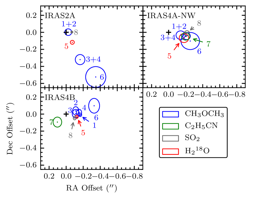
Figure 3: Positions of the lines from circular Gaussian fits in the ($uv$)-plane to the integrated line emission. The positions are plotted relative to the continuum peak position (cross) and the error in position for the continuum peak position is roughly the extent of the cross while the extent of the ellipses shows the error in position for the lines. Ellipses with the same colors represent the same molecule, while the numbers refer to a certain molecule and transition which has the same number in Fig. 1, Table 3, Table 5 and Table 6.2. Many of the detected lines are systematically offset from the continuum peak.

4.2 Water associated with the outflow in IRAS2A

Whereas the bulk of the H${}_{2}^{18}$O emission toward the three sources is associated with the central protostellar component, some extended emission at the velocity of the H${}_{2}^{18}$O line is seen extending toward the southwest in the integrated intensity map for IRAS2A (Fig. 2). Previous observations of IRAS2A have shown that it is oriented such that the outflow lobe extending in the SW direction is blueshifted (Jørgensen et al. 2004, 2007).

To investigate this emission further, continuum subtracted channel maps between 2 and 33 km s^-1, integrated in steps of 2.1 km s^-1, are shown in Fig. 4. Starting at the higher velocities, corresponding to SO₂ emission in Fig. 1, strong on-source emission is seen, but also the extended outflow emission. The gray lines trace the rough position of the peak outflow emission in the frames 5.0 to 32.0 km s^-1, corresponding to a linear velocity gradient characteristic for outflow affected material: the peak of the emission in each frame moves further away along the outflow when moving to more blue-shifted velocities. At 19.5 km s^-1 the knot identified as SO₂ has moved about 3″ away from the central source. The knot persists at this position (3$\sim$4″ away) almost throughout the rest of the maps and at a velocity of 5.0–7.1 km s^-1 it weakens. At 9.2 km s^-1 emission is seen to emerge close to the protostar, which is identified as H${}_{2}^{18}$O. It strengthens slightly and moves away from the source with lower velocities. Just as with the SO₂ emission it can be traced, although over a smaller number of channels and spatial extent (red line). The outflow water emission is extended and weak, but shows that water is present in the outflow of IRAS2A.

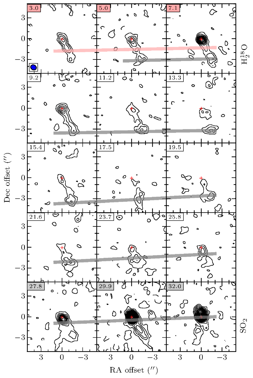
Figure 4: Continuum subtracted channel map between 2 and 33 km s^-1 for IRAS2A, velocity in km s^-1 given in each frame, channel width is 2.1 km s^-1. Contours in steps of 3$\sigma$ (24 mJy beam^-1 km s^-1) from a 3$\sigma$ level. The beam size is given in the lower left corner of the first frame. Gray and red broad lines trace the different outflow components of SO₂ and H${}_{2}^{18}$O, respectively .

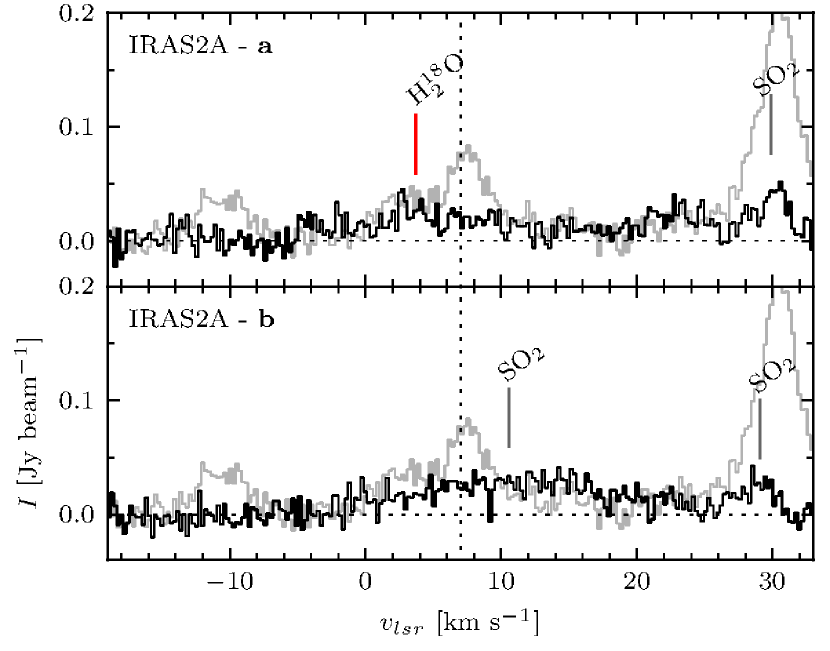
Figure 5: IRAS2A off-position spectra, averaged over 1″$\times$1″ regions around the positions marked with a and b in Fig. 2 in the blueshifted outflow from the imaged data. The spectra have been rebinned to twice the velocity resolution (width of 0.23 km s^-1). The systemic velocity of the H${}_{2}^{18}$O line is drawn with a vertical dotted line at $v_{\rm lsr}=7$ km s^-1, and the gray outline in the background is the on-source spectrum averaged in a region of the same size as the other spectra.

The detection of extended outflow H${}_{2}^{18}$O and SO₂ emission is further strengthened when looking at spectra at different positions in the outflow. Spectra extracted at two positions (averaged over 1″$\times$1″ regions) from the low surface brightness material in the outflow are shown in Fig. 5. In Fig. 2 the positions are marked with a (magenta cross) and b (green cross). Outflow position a shows one SO₂ component with a weak blue tail and a broad H${}_{2}^{18}$O component that is blueshifted 4–6 km s^-1 from the rest velocity. This blueshift coincides with the velocity of the CH₃OCH₃ lines 3 and 4, but the absence of the CH₃OCH₃ lines 1 and 2, which are detected in the on-source spectra, shows that it is indeed H${}_{2}^{18}$O. At position b only SO₂ with a broad blueshifted component and a narrow component is visible.

Thus the extended outflow emission seen towards IRAS2A in Fig. 2 is at least partly blueshifted H${}_{2}^{18}$O in the inner part, close to the source and SO₂ in the outermost part of the outflow.

4.3 Constraints on geometry and dynamics

Watson et al. (2007) suggested that the difference between IRAS4A and IRAS4B could be attributed to either hot water only being detectable during a short phase of the life cycle of YSOs or alternatively a particularly favorable line of sight in that system. Because of the lower dust opacity, protostellar envelopes are optically thin at submillimeter wavelengths, which allows detections of the water emission lines from the smallest scales towards the center of the protostars. The detections towards three of three targeted sources (Jørgensen & van Dishoeck 2010a, and this paper) therefore argue against the first of these suggestions.

The detected velocity gradient in IRAS4B – which is absent in the other sources (Fig. 2) – may be a geometrical effect. A simple solution could be that the sources without a velocity gradient are observed close to face-on. This would require that IRAS4B with its detected velocity gradient is observed edge-on, however. This is not supported by observations of the outflows (Jørgensen et al. 2007): all three sources show well-separated red and blue outflow cones suggesting at least some inclination of the outflows relative to the line-of-sight. Also, of the three sources, IRAS4B in fact shows the most compact outflow: if one assumes similar extents of the outflows this would suggest that IRAS4B rather than the other sources are seen more close to face-on.

Another way to deduce the inclination of the outflow with respect to the plane of the sky is through observations of maser spots in the outflows of the sources, although they do not seem to agree with observations of the larger scale outflow in many cases. Marvel et al. (2008) conclude that in IRAS4A-NW, the maser emission cannot be directly associated with the large scale outflow. For IRAS4B the masers have been associated with the outflow (Marvel et al. 2008; Desmurs et al. 2009), but the position angle of the “maser outflow” still differs from that of the CO outflow by some 20–30^∘.

We propose that the compact H${}_{2}^{18}$O emission has its origin in a flattened disk-like structure where inward motions is still dominating the dynamics, and where the viewing angle defines the observational characteristics (Fig. 6 for a schematic drawing). In fact, Brinch et al. (2009) suggest, based on modeling of submillimeter observations, that IRAS2A indeed has such a structure on a few 100 AU scales. Observing a source with this structure at different viewing angles would potentially produce the observed differences.

In the proposed solution, IRAS4B is viewed at an angle, closer to face-on, causing the mid-IR emission observed by Spitzer to escape from the envelope through the cavities produced by the outflow, where the optical depth along the line of sight is lower in agreement with the suggestion by Watson et al. (2007) (case A in Fig. 6). In IRAS2A and IRAS4A-NW, the viewing angle is closer to edge-on, causing mid-IR emission to be blocked by the optically thick envelope (case B in Fig. 6).

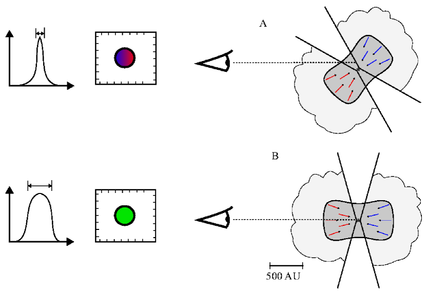
Figure 6: Schematic drawing of a disk dominated by inward motions rather than rotation in different observation geometries. In case A (IRAS4B), the observed line is narrow and a small velocity gradient is seen. In case B (IRAS2A and IRAS4A-NW), the observed line is broader and no velocity gradient is observed.

This solution could also explain the velocity gradient observed towards IRAS4B and the broader line widths towards IRAS2A and IRAS4A-NW. In disks dominated by inward motions rather than rotation, the systems viewed at an angle exhibit narrow lines and a velocity gradient (case A in Fig. 6), while systems viewed edge on show broader lines and no velocity gradient (case B in Fig. 6). The dynamical structure of the disk would move towards a rotationally supported disk on a local dynamical time-scale, which is a few $\times 10^{3}$ yr at a radius of 110 AU (Brinch et al. 2009).

4.4 Non-masing origin of H${}_{2}^{18}$O emission

We now turn the attention to chemical implications of the presented data: the subsequent analysis of the data focuses on the abundance and excitation of water and other species detected in the spectra.

The primary concern about the H${}_{2}^{18}$O analysis in this context is whether the H${}_{2}^{18}$O line could be masing. Many lines of water observable from the ground are seen to be masing, as is the case for the same transition studied here ($3_{1,3}-2_{2,0}$) but in the main isotopologue, H${}_{2}^{16}$O (Cernicharo et al. 1994). Several observables argue against that the H${}_{2}^{18}$O $3_{1,3}-2_{2,0}$ line is masing in the sources investigated here.

First, the line widths observed in the central beam towards the continuum peak are comparable for all the detected species in each of the sources, as was also seen in IRAS4B (Jørgensen & van Dishoeck 2010a, b). Although the mean line width is somewhat broader in IRAS2A and IRAS4A-NW compared to IRAS4B they are still significantly more narrow towards the central source (<5 km s^-1) than in the broad outflow components seen in the Herschel data (> 5 km s^-1) towards these sources (Kristensen et al. 2010). For IRAS2A, the mean FWHM and standard deviation of the fitted lines is 2.8$\pm$0.7 km s^-1, for IRAS4A-NW 2.4$\pm$1.0 km s^-1, and for IRAS4B 1.1$\pm$0.2 km s^-1. In addition to this, the variations in intensities between the different lines in each source are smaller than the variations in line intensity between the sources.

In IRAS2A, Furuya et al. (2003) report that maser emission at 22 GHz is highly variable and has a velocity of 7.2 km s^-1, i.e. marginally red-shifted. For IRAS4A, Furuya et al. (2003) and Marvel et al. (2008) show that the strongest maser component lies at $\sim$10 km s^-1 where we do not detect any strong H${}_{2}^{18}$O millimeter emission.

Taken together, these arguments suggest that the H${}_{2}^{18}$O emission detected towards the central positions of the sources is not masing, but instead is thermal emission with the same origin as the other detected species.

4.5 Column densities and abundances determinations

Having established that the H${}_{2}^{18}$O line is unlikely to be masing, the column densities for each species can be determined and compared directly. The emission from the different molecules is assumed to be optically thin and to uniformly fill the beam (valid since the deconvolved size in Table 3 is comparable to the beam size). The excitation is taken to be characterized by a single excitation temperature $T_{\mathrm{ex}}$, which does not have to be equal to the kinetic temperature.

4.5.1 Water column density and mass

Table 4 summarizes the inferred column densities of the various molecules assuming $T_{\mathrm{ex}}$=170 K. The gas-phase H₂O abundance and mass are calculated with an isotopic abundance ratio of ¹⁶O/¹⁸O of 560 in the local interstellar medium (Wilson & Rood 1994). The masses of gas phase H₂O in the sources are given in the bottom of Table 4, in units of Solar and Earth masses, along with the fraction of gas phase water relative to H₂. As pointed out by Jørgensen & van Dishoeck (2010a), in IRAS4B, the derived column density of H₂O is almost 25 times higher than deduced by Watson et al. (2007). The deduced mass of the gas phase water in IRAS2A is roughly six times higher than in IRAS4A-NW and 90 times higher than in IRAS4B. Thus, water is present in the inner parts of all of the sources and the non-detection in IRAS4A and IRAS2A at mid-infrared wavelengths is due to the high opacity of the envelope combined with a strong outflow contribution to H${}_{2}^{16}$O lines in IRAS4B (see also Herczeg et al. 2011).

Table 4: Derived properties of the detected species over the deconvolved sizes of the lines for all sources in the project.

	IRAS2A	IRAS4A-NW	IRAS4B
$N_{\mathrm{CH_{3}OCH_{3}}}$	1.2$\times 10^{17}$	6.8$\times 10^{16}$	5.6$\times 10^{16}$
$N_{\mathrm{H_{2}^{18}O}}$	2.9$\times 10^{16}$	7.9$\times 10^{15}$	3.9$\times 10^{15}$
$N_{\mathrm{C_{2}H_{5}CN}}$	$<$1.4$\times 10^{14}$	1.1$\times 10^{15}$	2.8$\times 10^{14}$
$N_{\mathrm{SO_{2}}}$	1.8$\times 10^{16}$	8.2$\times 10^{15}$	1.3$\times 10^{15}$
M${}_{\rm H_{2}O}$ ($M_{\rm\sun}$)	1.8$\times 10^{-6}$	2.7$\times 10^{-7}$	1.5$\times 10^{-8}$
M${}_{\rm H_{2}O}$ ($M_{\rm\oplus}$)	0.61	0.09	0.006
$X$(=$N_{\rm H_{2}O}/N_{\rm H_{2}}$)	4.2$\times 10^{-6}$	1.4$\times 10^{-7}$	7.8$\times 10^{-9}$

n cm^-2 assuming $T_{\mathrm{ex}}$=170 K. The typical error is a combination of the assumption of the excitation temperature and the flux calibration uncertainty ($\sim$20%). The determined column density varies with $T_{\mathrm{ex}}$ in the interval 100–200 K differently for each molecule, see Fig. 8 and the discussion in Sect. 4.5.3. sing only lines 1, 2, 3 and 4.

The ratio of H₂O gas phase abundance to the total H₂ abundance (derived from continuum observations (Jørgensen et al. 2009)) in Fig. 7 shows that the fractional abundance of gas phase water in IRAS2A is much higher than in IRAS4A-NW and IRAS4B. Still, the gas-phase water likely accounts for only a small fraction of the total amount of water (gas+ice) on those scales. Typical H₂O to H₂ abundance ratios of 10^-5 – 10^-4 have been deduced in shocked regions close to protostars (Harwit et al. 1998; Nisini et al. 1999), and in ices in the cold outer parts of protostellar envelopes (Pontoppidan et al. 2004). In shocks, high temperature gas-phase reactions drive much of the oxygen into water (Draine et al. 1983). In more quiescent regions the ice is expected to evaporate off the grains when heated to temperatures above 100 K in close proximity to the central source (Fraser et al. 2001). The fact that our inferred abundance ratios are generally much lower than 10^-4 suggests that a large fraction of the dust mass in the inner $\sim$100 AU has a temperature below 100 K, with the fraction varying from source to source. In colder regions, most of the water gas originates from UV photodesorption of ices. Assuming a total H₂O to H₂ abundance ratio of 10^-4 (gas+ice), the fraction of water in the gas phase is 4% for IRAS2A, 0.1% for IRAS4A-NW and 0.01% for IRAS4B of the total water content (gas+ice). This difference could be due, for example, to varying intensities of the UV radiation from the newly formed stars and geometry causing differences in the relative amounts of material heated above the temperature where water ice mantles are evaporated. Towards the more evolved Class II source TW Hydra, Hogerheijde et al. (2011) deduce a gas phase water to total hydrogen abundance of 2.4$\times 10^{-8}$ using Herschel. This value is of the same order of magnitude as our results, and places TW Hydra just above IRAS4B in Fig. 7.

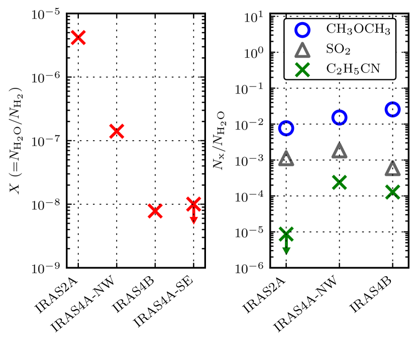
Figure 7: Left: Fraction of gas phase water relative to H₂ (from the continuum observations of Jørgensen et al. 2009) for the different sources, including an upper limit estimate for IRAS4A-SE. Right: Ratio of the column density of the molecules relative to water. The C₂H₅CN value for IRAS2A is an upper limit.

4.5.2 Other molecules

In the right plot of Fig. 7, the abundances of the detected molecules relative to H₂O are presented. The CH₃OCH₃ and SO₂ content relative to H${}_{2}^{18}$O is roughly comparable between the different sources. This suggests that for CH₃OCH₃, SO₂ and H${}_{2}^{18}$O (and thus H₂O) similar chemical processes are at work in the three sources. C₂H₅CN is the least abundant of the molecules for all the sources. In IRAS2A the high abundance of water is contrasted by the relatively low abundance of C₂H₅CN, for which only an upper limit is deduced. This relatively low abundance in IRAS2A is robust even when much lower excitation temperatures are assumed (see Sect. 4.5.3).

It is also evident from Fig. 7 and Table 4 that the CH₃OCH₃/C₂H₅CN column density ratio varies significantly between the sources. This ratio is 10³ for IRAS2A, 60 for IRAS4A-NW and 200 for IRAS4B assuming $T_{\mathrm{ex}}$=170 K. The differences in relative abundances of N and O-bearing complex organics have been interpreted as an indicator for different physical parameters (Rodgers & Charnley 2001) and different initial grain surface composition (Charnley et al. 1992; Bottinelli et al. 2004). Caselli et al. (1993) argue that the (dust) temperature history of the cloud, in particular whether it was cold enough to freeze out CO, is an important factor for the resulting ratio.

4.5.3 Effect of excitation temperature

The results presented in Sections 4.5.1 and 4.5.2 assume an excitation temperature of 170 K for all species. In this section we demonstrate that all our conclusions are robust over a wide range of assumed temperatures. The adopted $T_{\mathrm{ex}}$=170 K is the same as found from the model fit to the mid-infrared water lines observed by Spitzer (Watson et al. 2007) and allows for easy comparison to this paper and Jørgensen & van Dishoeck (2010a).

Although the origin of the mid-infrared and millimeter lines are likely not the same, this temperature is a reasonable first guess appropriate of the conditions in the inner 150 AU of protostellar systems. From modeling of dust continuum observations, the density in the inner envelope/disk is found to be high, at least 10⁷ cm^-3, and the dust temperature is thought to be at least 90 K for a fraction of the material (e.g., Jørgensen et al. 2002, 2004). This is also the temperature at which water is liberated from the grains; any gas-phase water detected in the high excitation line observed here ($E_{\mathrm{u}}$$\approx$200 K) likely originates from the warmer regions (Sect. 4.5.1).

The current observations and literature data do not provide enough information on the line emission at these scales to constrain the excitation temperature directly. For none of the detected species are there more than two previous measurements and those detections either have large uncertainties due to their weakness (Jørgensen et al. 2005) or are sensitive to larger scale emission including outflow and envelope because of the large beam (Bottinelli et al. 2004, 2007; Wakelam et al. 2005). For the deeply embedded low-mass protostar IRAS 16293-2422, Bisschop et al. (2008) derive rotational temperatures between 200–400 K from several compact emission lines of complex molecules using SMA data. Furthermore, for the outflow toward IRAS4B Herczeg et al. (2011) deduce $T_{\mathrm{ex}}$=110–220 K with recent Herschel PACS data.

Figure 8 explores what happens with the column densities at significantly different excitation temperatures than those assumed here. It shows two different plots for the three sources. The plots in the top row show the ratio between the column density of the various molecules and that of water, whereas the plots in the bottom row show the column densities themselves, all as functions of excitation temperature. The ratios ($N_{\mathrm{X}}/N_{\mathrm{H_{2}O}}$) do not change significantly between 100 and 275 K. The gray area in the lower plots shows the range of excitation temperatures for which the column density of water is the same in the three sources. Only if the excitation temperature in IRAS4A-NW and IRAS4B is lower than 50 K can all sources have comparable water column densities based on the observed intensities.

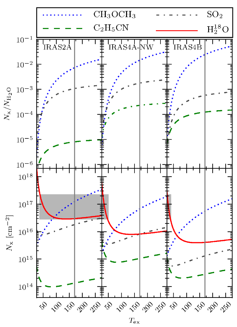
Figure 8: Plots showing (upper) the ratio between the detected molecules and water (H₂O), assuming that the species have the same $T_{\mathrm{ex}}$ and (lower) the column density of all the detected lines (including H${}_{2}^{18}$O). The colors and line style indicate the different molecules, the gray vertical line mark $T_{\mathrm{ex}}$= 170 K and the gray area in each plot indicate the temperatures where the column density of H${}_{2}^{18}$O is the same for the sources.

The different molecules could of course each have different excitation temperatures. Specifically, can different excitation temperatures be the cause of the large range in inferred CH₃OCH₃/C₂H₅CN column density ratios? Figure 9 shows this ratio and the individual column densities for excitation temperatures from 25 to 275 K for IRAS2A. The corresponding plots for the other two sources show similar trends (see also Fig. 8). The temperature does not affect the column density estimate for C₂H₅CN significantly, showing that our upper limit estimate is rather robust, and that the differences in this ratio between the sources cannot be attributed to differences in the excitation of C₂H₅CN alone. On the other hand, changing the excitation temperature for CH₃OCH₃ affects the column density and the ratio to a greater extent. This difference in behavior with $T_{\mathrm{ex}}$ for the two molecules is caused by the transitions’ upper energy levels ($E_{\mathrm{u}}$); 18 K for CH₃OCH₃ versus 122 K for C₂H₅CN. For CH₃OCH₃, its lower value of $E_{\mathrm{u}}$ causes the column density estimate to decline more rapidly with $T_{\mathrm{ex}}$ than for C₂H₅CN: the contribution from the exponent in the Boltzmann distribution (exp(–$E_{\mathrm{u}}$/k$T_{\mathrm{ex}}$)) does not compensate for the fall that the partition function (proportional to $T_{\mathrm{ex}}$^b, where $b$>0) introduces. In the temperature range 40 to 250 K the CH₃OCH₃/C₂H₅CN column density ratio varies with a factor of about 30. Looking only at the CH₃OCH₃/C₂H₅CN column density ratio, the excitation temperature for IRAS2A has to be $T_{\mathrm{ex}}$=45 K, and for IRAS4B $T_{\mathrm{ex}}$=85 K, to match that of IRAS4A-NW.

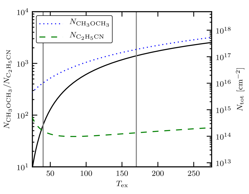
Figure 9: Plot of the ratio between CH₃OCH₃ and C₂H₅CN in IRAS2A (left $y$-axis, filled line), and the column densities derived for those molecules (right $y$-axis, dashed/dash dotted line) for temperatures between 25 and 275 K. The vertical lines show $T$=40 and 170 K.

As argued above based on the physical characteristics of the sources, values of $T_{\mathrm{ex}}$ significantly below 100 K and large differences in $T_{\mathrm{ex}}$ between molecules and sources are not expected on the scales probed here. Also, the agreement in widths, extent and positions between the lines argues against this. If the temperature is allowed to vary in the range 100-250 K the conclusions drawn in this paper are unchanged.

4.6 Formation of molecules in the protostellar environment

The simultaneous observations of water and the complex molecules can also be used to shed new light onto where and how the formation of various molecules takes place in the protostellar environment. The basic scenario is that many of the complex organic molecules are formed as a result of grain-surface reactions during the collapse of the protostellar envelopes as material is heated slowly (see Herbst & van Dishoeck 2009, for a review).

Garrod & Herbst (2006) use a gas-grain network of reactions to investigate the formation of certain complex organic molecules in hot cores and corinos during the warm-up and evaporative stages. The results show that the chemistry occurs both on grain surfaces and in the gas phase, with the two phases being strongly coupled with each other. Large abundances of complex organic molecules are present at the end of this warm-up stage, and show that a period of 10⁴ – 10⁵ years is vital for the formation of complex molecules.

A key question is thus whether the material in these low-mass protostars spends enough time at moderate temperatures of 20–40 K to form complex organic molecules during the collapse of the cloud and formation of the disk. A parcel of material originating in the cold core will pass through the warm inner envelope during the collapse and be incorporated into the disk before being accreted onto the star. Depending on its precise origin, the material can follow many different routes, but exploration of a variety of collapse models shows that most parcels indeed spend the required period at moderate temperatures to form the complex organics, either in the inner envelope or in the disk (Visser et al. 2009). Some of the routes result in the material being directly exposed to UV radiation near the outflow cavity walls (Visser et al. 2012). After evaporation, gas-phase temperatures in the hot core are generally too low (i.e., $T\lesssim 230$ K, $R\gtrsim 20$ AU, Larson 1972; Jørgensen et al. 2002) for any significant gas-phase formation of water to take place. The fact that we observe narrow emission lines of complex molecules on small scales confirms that some fraction of the collapsing cloud has spent enough time under conditions that lead to the formation of complex species that will enter the disk.

5 Summary and Outlook

We have presented subarcsecond resolution observations of the H${}_{2}^{18}$O $3_{1,3}-2_{2,0}$ transition at 203.4 GHz towards a small selection of deeply embedded protostars in the NGC 1333 region. In addition to the targeted H${}_{2}^{18}$O molecule, SO₂ and complex organic molecules are seen.

• Water is successfully detected towards IRAS2A and one component of the IRAS4A binary. These data add to the previous detection of the $3_{1,3}-2_{2,0}$ transition of H${}_{2}^{18}$O towards IRAS4B by Jørgensen & van Dishoeck (2010a). The origin of the emission differs from that seen with both Herschel and Spitzer, where larger-scale emission (protostellar envelope, outflow shocks/cavity walls) is detected.

• The gas-phase water abundance is significantly lower than a canonical abundance of 10^-4, suggesting that most water is frozen out on dust grains at these scales. The fraction of water in the gas phase is 4% for IRAS2A, 0.1% for IRAS4A-NW and 0.01% for IRAS4B of the total water content (gas+ice).

• IRAS2A shows H${}_{2}^{18}$O eission not only at the source position, but also in the blueshifted outflow. In IRAS4A we only detect water towards IRAS4A-NW. None of the lines presented for the other sources are detected towards IRAS4A-SE.

• Based on the small species-to-species variations, in both line strength and line width, we argue that the H${}_{2}^{18}$O $3_{1,3}-2_{2,0}$ emission line is not masing in these environments and on these scales.

• While IRAS4B shows narrow emission lines and a tentative velocity gradient, reported by Jørgensen & van Dishoeck (2010a), the other sources show broader lines and no velocity gradients. Additionally, IRAS4B is the only source of the three detected in mid-infrared water lines by Watson et al. (2007). We propose that a disk-like structure dominated by inward motions rather than rotation with different orientations with respect to the observer could explain the observed line characteristics.

• The abundances of the detected molecules differ between the sources: the abundance of C₂H₅CN with respect to water, compared to both SO₂ and CH₃OCH₃, is much lower in IRAS2A than the other sources. This shows that the formation mechanism for C₂H₅CN is different from the other molecules, indicating that it is not trapped in the water ice mixture or related to the sublimation of water.

The detections of H${}_{2}^{18}$O emission from the ground show good promise for using H${}_{2}^{18}$O as a probe of the inner regions of protostars and for studying the formation of complex organic molecules in the water-rich grain ice mantles. Higher resolution observations, using the PdBI in the most extended configuration, or with the Atacama Large Millimeter/submillimeter Array (ALMA) band 5 could be used to reveal the kinematical structure of the 10–100 AU scales and the dynamics of the forming disks. Observations of higher excited lines of H${}_{2}^{18}$O and the complex organics in other ALMA bands (e.g., band 8) could provide a better handle on the excitation conditions of water on few hundred AU scales in the centers of protostellar envelopes. Finally, observing more protostellar sources in the H${}_{2}^{18}$O $3_{1,3}-2_{2,0}$ transition would provide a better statistical sample for comparisons and conclusions.

Appendix A Tables

Table 5: Tabulated data for the different lines detected from JPL (Pickett et al. 1998) and CDMS (Müller et al. 2001).

No.	Molecule	Transition	Rest Freq.	$E_{\mathrm{u}}$	$\log{A_{ij}}$
			(GHz)	(K)	($\log s^{-1}$)
1	CH3OCH3	33,0 – 22,1 EE	203.4203	18.1	-4.61
2	CH3OCH3	33,0 – 22,1 AA	203.4187	18.1	-4.23
3	CH3OCH3	33,0 – 22,1 AE	203.4114	18.1	-4.23
4	CH3OCH3	33,1 – 22,1 EE	203.4101	18.1	-4.46
5	H${}_{2}^{18}$O	31,3 – 22,0	203.4075	203.7	-5.32
6	CH3OCH3	33,1 – 22,1 EA	203.4028	18.1	-4.39
7	C2H5CN	232,22 – 222,21	203.3966	122.3	-3.15
8	SO2	120,12 – 111,11	203.3916	70.1	-4.07

Table 6: Position and FWHM of the detected lines from Gaussian fits to the spectra.

			IRAS2A				IRAS4A-NW
No.	Molecule	Position	Width	Interval		Position	Width	Interval
		(km s-1)	(km s-1)	(km s-1)		(km s-1)	(km s-1)	(km s-1)
1	CH3OCH3	$-11.7\pm 0.1$	$2.3\pm 0.1$	$-14.0--7.0$		$-11.3\pm 0.1$	$1.6\pm 0.1$	$-13.0--7.3$
2	CH3OCH3	$-9.3\pm 0.1$	$2.3\pm 0.1$	$-$		$-9.0\pm 0.1$	$1.6\pm 0.1$	$-$
3	CH3OCH3	$+1.3\pm 0.1$	$2.3\pm 0.1$	$-1.0-+4.4$		$+1.7\pm 0.1$	$1.6\pm 0.1$	$0.0-+4.7$
4	CH3OCH3	$+3.2\pm 0.1$	$2.3\pm 0.1$	$-$		$+3.6\pm 0.1$	$1.6\pm 0.1$	$-$
5	H${}_{2}^{18}$O	$+7.4\pm 0.1$	$4.0\pm 0.1$	$+4.4-+11.4$		$+6.6\pm 0.1$	$2.9\pm 0.3$	$+4.7-+9.6$
6	CH3OCH3	$+15.2\pm 0.2$	$2.3\pm 0.1$	$+12.9-+17.5$		$+14.4\pm 0.1$	$1.6\pm 0.1$	$+12.0-+15.2$
7	C2H5CN	$-$	$-$	$-$		$+22.8\pm 0.2$	$3.8\pm 0.4$	$+19.0-+26.9$
8	SO2	$+30.4\pm 0.1$	$3.8\pm 0.1$	$+26.6-+33.9$		$+30.4\pm 0.1$	$4.1\pm 0.2$	$+26.9-+34.6$