Trajectories in a space with a spherically symmetric dislocation

Abstract. We consider a new type of defect in the scope of linear elasticity theory, using geometrical methods. This defect is produced by a spherically symmetric dislocation, or ball dislocation. We derive the induced metric as well as the affine connections and curvature tensors. Since the induced metric is discontinuous, one can expect ambiguity coming from these quantities, due to products between delta functions or its derivatives, plaguing a description of ball dislocations based on the Geometric Theory of Defects. However, exactly as in the previous case of cylindric defect, one can obtain some well-defined physical predictions of the induced geometry. In particular, we explore some properties of test particle trajectories around the defect and show that these trajectories are curved but can not be circular orbits.

Keywords: Dislocation, Spherical Symmetry, Linear Elasticity Theory, Gravity.

1 Introduction

The topological defects attract great interest due to the applications to condensed matter physics (see, e.g., [1, 2] for an introduction and recent review). Another elegant approach in this area is the geometric theory of defects [3, 4] (see also [5] for the introduction), which is formulated in terms of the notions originally developed in the theories of gravity. In this framework, we can cite basically two kinds of defects, described in the view of Riemann-Cartan geometry: disclinations and dislocations. This means that the curvature and torsion tensors, respectively, are interpreted as surface densities of Frank and Burgers vectors and thus linked to the nonlinear, generally inelastic deformations of a solid. Recently, the qualitatively new kind of geometric defect has been described in [6] (see also [7]), corresponding to a tube dislocation (with cylindrical symmetry).

Nevertheless, one can find others well known types of dislocations. In Elasticity Theory, the dislocations and their physical effects are a matter of great concern, specially the screw dislocation [8]. In this paper, we consider a ball dislocation (or sphere dislocation), which is the same type of defect studied in [6], translated to spherical symmetry. Is is remarkable that such a problem was not investigated yet. For our purposes, the approach will be limited to linear elasticity theory (using Riemann-Cartan geometry as a tool). The ball dislocation can be understood by the illustration in Figure 1.

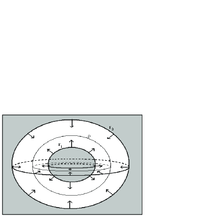
Figure 1: Ball dislocation produced by cutting a spherical sector, and then indentifying the surfaces $r_{1}$ and $r_{2}$ with $\rho$.

It is possible to treat this defect as a point defect in the limiting case where $\rho$ is much smaller than the dimensions of the considered physical system. Of course, the ball dislocation provides a more general picture. This paper is organized in the following way. In Section 2, we treat mathematically the ball dislocation, find the solution of the variable which describes the defect, and with the help of Gravity Theory methods, we study the trajectories of test particles in Section 3. Finally we proceed to our conclusions.

2 Ball dislocation in linear elasticity theory

Let us describe the ball dislocations in linear elasticity theory. Consider a homogeneous and isotropic elastic media as a three-dimensional Euclidean space ${\mathbb{R}}^{3}$ with Cartesian coordinates $\,x^{i},\,y^{i}$, where $\,i=1,2,3$. The Euclidean metric is denoted by $\delta_{ij}={\rm diag}(+++)$. The basic variable in the elasticity theory is the displacement vector of a point in the elastic media, $u^{i}(x)$, $\,x\in{\mathbb{R}}^{3}$. In the absence of external forces, Newton’s and Hooke’s laws reduce to three second order partial differential equations which describe the equilibrium state of elastic media (see, e.g., [9]),

$$(1-2\sigma)\Delta u_{i}+\partial_{i}\partial_{j}u^{j}=0\,.$$ (1)

Here $\Delta$ is the Laplace operator and the dimensionless Poisson ratio $\sigma$  ($-1\leq\sigma\leq 1/2$)  is defined as

$$\sigma=\frac{\lambda}{2(\lambda+\mu)}\,.$$

The quantities $\lambda$ and $\mu$ are called the Lame coefficients, which characterize the elastic properties of media.

Raising and lowering of Latin indices can be done by using the Euclidean metric, $\delta_{ij}$, and its inverse, $\delta^{ij}$. Eq. (1) together with the corresponding boundary conditions enable one to establish the solution for the field $u^{i}(x)$ in a unique way.

Let us pose the problem for the ball dislocation shown in Figure 1. This dislocation can be produced as follows. We cut out the thick spherical sector of media located between two concentric spherical surfaces of radii $r_{1}$ and $r_{2}$ ($r_{1}<r_{2}$), move symmetrically both cutting surfaces one to the other and finally glue them. Due to spherical symmetry of the problem, in the equilibrium state the gluing surface is also spherical, of radius $\rho$ which will be calculated below.

Within the procedure described above and shown in Figue 1, we observe the negative ball dislocation because part of the media was removed. This corresponds to the case of $r_{1}<r_{2}$. However, the procedure can be applied in the opposite way by addition of extra media to ${\mathbb{R}}^{3}$. In this case, we meet a positive ball dislocation and the inequality has an opposite sign, $r_{1}>r_{2}$.

Let us calculate the radius of the equilibrium configuration, $\rho$. This problem is naturally formulated and solved in spherical coordinates, $\,r,\,\theta,\,\phi$. Let us denote the displacement field components in these coordinates by $\,u^{r},\,u^{\theta},\,u^{\phi}$. In our case, $\,u^{\theta}=u^{\phi}=0\,$ due to the symmetry of the problem, so that the radial displacement field $u^{r}(r)$ can be simply denoted as $\,u^{r}(r)=u(r)$.

The boundary conditions for the equilibrium ball dislocation are

$$u\big{|}_{r=0}=0\,,\qquad u\big{|}_{r=\infty}=0\,,\qquad\left.\frac{du_{\text{in}}}{dr}\right|_{r=r_{*}}=\left.\frac{du_{\text{ex}}}{dr}\right|_{r=r_{*}}\,.$$ (2)

The first two conditions are purely geometrical, and the third one means the equality of normal elastic forces inside and outside the gluing surface in the equilibrium state. The subscripts “in” and “ex” denote the displacement vector field inside and outside the gluing surface, respectively.

Let us note that our definition of the displacement vector field follows [5], but differs slightly from the one used in many other references. In our notations, the point with coordinates $y^{i}$, after elastic deformation, moves to the point with coordinates $x^{i}$:

$$y^{i}\rightarrow x^{i}(y)=y^{i}+u^{i}(x)\,.$$ (3)

The displacement vector field is the difference between new and old coordinates, $u^{i}(x)=x^{i}-y^{i}$. Indeed, we are considering the components of the displacement vector field, $u^{i}(x)$, as functions of the final state coordinates of media points, $x^{i}$, while in other references they are functions of the initial coordinates, $y^{i}$. The two approaches are equivalent in the absence of dislocations because both sets of coordinates $x^{i}$ and $y^{i}$ cover the entire Euclidean space ${\mathbb{R}}^{3}$. On the contrary, if dislocation is present, the final state coordinates $x^{i}$ cover the whole ${\mathbb{R}}^{3}$ while the initial state coordinates cover only part of the Euclidean space lying outside the thick sphere which was removed. For this reason the final state coordinates represent the most useful choice here.

The elasticity equations (1) can be easily solved for the case of ball dislocation under consideration. Using the Christoffel symbols in order to evaluate the expressions for the differential operators (Laplacian and divergence), equations (1) reduce to the only one non-trivial equation

$$\frac{d^{2}u(r)}{dr^{2}}+\frac{2}{r}\frac{du(r)}{dr}-\frac{2}{r^{2}}u(r)=0\,.$$ (4)

One can remember that only the radial component differs from zero. The angular $\theta$ and $\phi$ components of equations (1) are identically satisfied. The general solution for (4) is given by

$$u=\alpha r-\frac{\beta}{r^{2}}\,,$$ (5)

which depends on the two arbitrary constants of integration $\alpha$ and $\beta$. Due to the first two boundary conditions (2), the solutions inside and outside the gluing surface are

$$\begin{aligned} u_{\text{in}}&=\alpha r\,,\quad&\alpha&>0,\\ u_{\text{ex}}&=-\frac{\beta}{r^{2}}\,,\quad&\beta&>0.\end{aligned}$$ (6)

The signs of the integration constants correspond to the negative ball dislocation. For positive ball dislocation, both integration constants have opposite signs.

Using the solution (5) and the third boundary condition (2), one can determine the radius of the gluing surface,

$$\rho=\frac{2r_{2}+r_{1}}{3}.$$ (7)

One can see that $\rho$ is not the mean between $r_{1}$ and $r_{2}$, as it is for the cylindrical symmetry defect [6]. On the contrary, the gluing surface is located closer to the external radius $r_{2}$. After simple algebra, the integration constants can be expressed in terms of $\rho$ and the thickness of the sphere $l=r_{2}-r_{1}$:

$$\alpha=\frac{2l}{3\rho}\qquad\beta=\frac{\rho^{2}l}{3}\,.$$ (8)

It is straightforward also to get

$$r_{1}=\frac{3\rho-2l}{3}\;\;{\rm and}\;\;r_{2}=\frac{3\rho+l}{3}\,.$$

Observe that as $r_{1}$ is positive, we must have always $\rho>2l/3$.

Finally, within the linear elasticity theory, eq. (6) with the integration constants (8) yields a complete solution for the ball dislocation in linear elasticity theory, valid for small relative displacements, when  $l/r_{1}\ll 1$ and $l/r_{2}\ll 1$. It is remarkable that the solution obtained in the framework of linear elasticity theory does not depend on the Poisson ratio of the media. In this sense, the ball dislocation is a purely geometric defect which does not feel the elastic properties.

In order to use the geometric approach, we compute the geometric quantities of the manifold corresponding to the ball dislocation. From the geometric point of view, the elastic deformation (3) is a diffeomorphism between the given domains in the Euclidean space. The original elastic media ${\mathbb{R}}^{3}$, before the dislocation is made, is described by Cartesian coordinates $y^{i}$ with the Euclidean metric $\delta_{ij}$. An inverse diffeomorphic transformation $x\rightarrow y$ induces a nontrivial metric on ${\mathbb{R}}^{3}$, corresponding to the ball dislocation. In Cartesian coordinates, this metric has the form

$$g_{ij}(x)\,=\,\frac{\partial y^{k}}{\partial x^{i}}\,\frac{\partial y^{l}}{\partial x^{j}}\,\delta_{kl}.$$ (9)

We use curvilinear spherical coordinates for the ball dislocation and therefore it is useful to modify our notations. The indices in curvilinear coordinates in the Euclidean space ${\mathbb{R}}^{3}$ will be denoted by Greek letters $\,x^{\mu}$, $\mu=1,2,3$. Then the “induced” metric for the ball dislocation in spherical coordinates is

$$g_{\mu\nu}(x)\,=\,\frac{\partial y^{\rho}}{\partial x^{\mu}}\,\frac{\partial y^{\sigma}}{\partial x^{\nu}}\,\,\overset{\circ}{g}_{\rho\sigma}\,,$$ (10)

where $\overset{\circ}{g}_{\rho\sigma}$ is the Euclidean metric written in spherical coordinates. We denote spherical coordinates of a point before the dislocation is made by $\{y,\theta,\phi\}$, where $y$ without index stands for the radial coordinate and we take into account that the coordinates $\theta$ and $\phi$ do not change. Then the diffeomorphism is described by a single function relating old and new radial coordinates of a point, $y=r-u(r)$, where

$$u(r) = \frac{2l}{3\rho}r\,,\quad r<\rho$$ (11)

$$u(r) = -\frac{\rho^{2}l}{3r^{2}}\,,\quad r>\rho\,.$$ (12)

It is easy to see that this function has a discontinuity $u_{\rm ext}-u_{\rm int}|_{r=\rho}=l$ at the point of the cut. Therefore a special care must be taken in calculating the components of induced metric.

It is useful to express $u(r)$ in a way simultaneously valid in both domains, $r<\rho$ and $r>\rho$. We have then

$$u(r)=\frac{2l}{3\rho}rH(\rho-r)-\frac{\rho^{2}l}{3r^{2}}H(r-\rho)\,,$$ (13)

where $H(r-\rho)$ is the Heaviside step function. As $H^{\prime}(r-\rho)=\delta(r-\rho)$, one achieves

$$u^{\prime}(r)=\frac{du(r)}{dr}=v(r)-l\delta(r-\rho)\,,$$ (14)

where

$$v(r)=\frac{2l}{3\rho}H(\rho-r)+\frac{2\rho^{2}l}{3r^{3}}H(r-\rho)\,.$$

By direct calculation of induced metric, by (10), one can write the corresponding line element as

$$ds^{2}=(1-u^{\prime})^{2}dr^{2}+(r-u)^{2}(d\theta^{2}+\sin^{2}\theta d\phi^{2})\,.$$ (15)

It is clear that the above expression, besides discontinuous, contains also a $\delta$-function thanks to $u^{\prime}$. In order to avoid further conceptual consequences coming from a $\delta$-function in the line element, we shall drop it, and adopt $u^{\prime}(r)\to v(r)$. In other words, let us consider the line element

$$ds^{2}_{{\rm int}} = \left(1-\frac{2l}{3\rho}\right)^{2}(dr^{2}+r^{2}d\theta^{2}+r^{2}\sin^{2}\theta d\phi^{2})\,,$$

$$ds^{2}_{{\rm ext}} = \left(1-\frac{2\rho^{2}l}{3r^{3}}\right)^{2}dr^{2}+\left(1+\frac{\rho^{2}l}{3r^{3}}\right)^{2}(r^{2}d\theta^{2}+r^{2}\sin^{2}\theta d\phi^{2})\,.$$

Notice that the interior space is conformally flat, with a constant scale factor, while the exterior metric is not so. Both metrics are flat (as follows by direct calculation of Riemann tensor), as they should be (because they were obtained by coordinate transformations starting from the Euclidean metric). Nevertheless, the whole space is non-trivial since curvature is non-trivial exactly in the gluing surface. Next, we are going to investigate the consequences for trajectories of test particles around the defect.

3 Trajectories of test particles around the defect

What are the trajectories of test particles in a space with such a defect? Of course, the trajectories without defect would be straight lines, so we expect deviation from straight lines in the actual path. How these trajectories can be described? Are there any possible closed path around the defect? In order to answer these questions, let us consider the geodesic equations for both metrics, in the interior and in the exterior of gluing surface. The geodesic equations read

$$\frac{dU^{\mu}}{d\tau}+\Gamma^{\mu}\mbox{}_{\rho\lambda}U^{\rho}U^{\lambda}=0\,,$$ (16)

where $U^{\mu}=dx^{\mu}/d\tau=(1,\,\dot{r},\,\dot{\theta},\,\dot{\phi})$ ($c=1$ and dot means derivative with respect to $\tau$) and

$$\Gamma^{\mu}\mbox{}_{\rho\lambda}=\frac{1}{2}g^{\mu\sigma}\left(\partial_{\lambda}g_{\sigma\rho}+\partial_{\rho}g_{\sigma\lambda}-\partial_{\sigma}g_{\rho\lambda}\right)\,.$$

Let us remmember that if only dislocations are present, then only torsion (without Riemannian curvature) is found in the geometric approach – only the Burgers vector is non-trivial. But for practical purposes, one can treat the problem in the reverse way, considering only Riemannian curvature, because both approaches are equivalent. This equivalence is very well-known in telleparalelism (see, e.g., [10]).

Inside the defect, the geodesics are straight lines and thus we shall consider only the exterior metric. By direct calculation, the geodesic equations, outside the gluing surface, can be written as

$$\ddot{r}+\frac{6\rho^{2}l}{r(3r^{3}-2\rho^{2}l)}\dot{r}^{2}-\frac{r(\rho^{2}l+3r^{3})}{3r^{3}-2\rho^{2}l}\left(\dot{\theta}^{2}+\sin^{2}\theta\dot{\phi}^{2}\right)=0\,,$$ (17)

$$\ddot{\theta}-\frac{4\rho^{2}l-6r^{3}}{r(\rho^{2}l+3r^{3})}\dot{r}\dot{\theta}-\sin\theta\cos\theta\dot{\phi}^{2}=0\,,$$ (18)

$$\ddot{\phi}-\frac{4\rho^{2}l-6r^{3}}{r(\rho^{2}l+3r^{3})}\dot{r}\dot{\phi}+\frac{2\cos\theta}{\sin\theta}\dot{\phi}\dot{\theta}=0\,.$$ (19)

The denominator appearing on (17) is always positive, because from condition $\rho>2l/3$, one gets $3r^{3}-2\rho^{2}l>3r^{3}-3\rho^{3}>0$.

An interesting feature that we can understand is that, if $\dot{r}=0$, then the test particle should be necessarily at rest. This follows from equation (17). This means that if the test particle is moving, so its radial coordinate must be changing: there is no possible trajectory confined in a spherical surface. In other words, one can say that such a geometrical defect can not serve as an alternative description of gravitating objects (around which we know there are permitted circular orbits). However, other kinds of effects, in condensed matter physics, for example, can not be ruled out.

A test particle can follow also a radial path, defined as any trajectory described by $\dot{\theta}=\dot{\phi}=0$. To see that, let us consider $\dot{\theta}=\dot{\phi}=0$, such that the radial equation (17) reads

$$\ddot{r}=-\frac{6\rho^{2}l}{r(3r^{3}-2\rho^{2}l)}\dot{r}^{2}\,,$$

which can be solved as

$$\dot{r}=\frac{Kr^{3}}{3r^{3}-2\rho^{2}l}\,,$$ (20)

where $K$ is an arbitrary integration constant. This trajectory is a straight line, and the particle’s radial velocity is such that it has greater absolute values near the defect. This effect is illustrated in Figure 2, where we plot the coordinate $r(t)$ against $t$ (the coordinate system is centered at the defect), based on the integration of (20),

$$r+\frac{\rho^{2}l}{3r^{2}}+a\tau+b=0\,,$$

where $a$ and $b$ are integration constants. We see in Figure 2 the effect of decreasing the absolute velocity as particle gets away from the defect (if there was no defect, the curve would be a straight line). Notice that as much the particle is away from the defect, its velocity approaches a constant value, as one should expect (for $r>>\rho$, kinematics is the same from a space without defect).

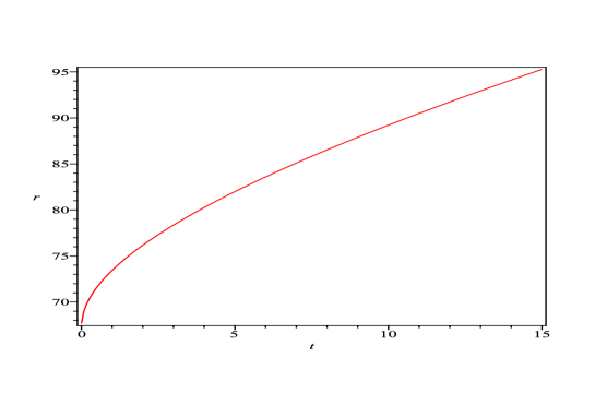
Figure 2: Radial curve for $\rho=\frac{203}{3}$ and $\dot{r}_{0}=50$.

To conclude, let us consider $\theta=\pi/2$ ($\dot{\theta}=0$) and $\dot{\phi}\neq 0$. The geodesic equations read

$$\ddot{r}+\frac{6\rho^{2}l}{r(3r^{3}-2\rho^{2}l)}\dot{r}^{2}-\frac{r(\rho^{2}l+3r^{3})}{3r^{3}-2\rho^{2}l}\dot{\phi}^{2}=0\,,$$ (21)

$$\ddot{\phi}-\frac{4\rho^{2}l-6r^{3}}{r(\rho^{2}l+3r^{3})}\dot{r}\dot{\phi}=0\,.$$ (22)

The last equation can be integrated and we obtain

$$\dot{\phi}=\frac{Ar^{4}}{(3r^{3}+\rho^{2}l)^{2}}\,,$$ (23)

where $A$ is some integration constant. Far away from the defect, we see that $\dot{\phi}$ is proportional to $r^{-2}$.

Substituting (23) into (21), we have

$$\ddot{r}+\frac{6\rho^{2}l}{r(3r^{3}-2\rho^{2}l)}\dot{r}^{2}-\frac{r(\rho^{2}l+3r^{3})}{3r^{3}-2\rho^{2}l}\frac{A^{2}r^{8}}{(3r^{3}+\rho^{2}l)^{4}}=0\,.$$

The above equation can be numerically integrated, and we can learn that the behavior of radial velocity is very similar to the one described by (20), which can be seen in Figure 3 (both drawn with the help of MAPLE software).

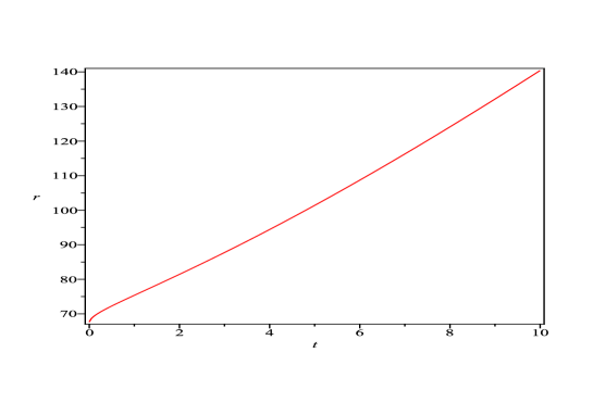
Figure 3: Radial curve for $\rho=\frac{203}{3}$ and $\dot{r}_{0}=50$.

One can extract an interesting information from (23), together with the natural assumption that the absolute velocity decreases in time (as suggested by (20)). As the solution $\dot{\phi}=(A/9)r^{-2}$ corresponds to straight lines (geodesics in flat space without defect), the actual derivative $\dot{\phi}$ given by (23) decays more slowly comparing to the straight line case. This means that the actual path must deviate from a straight line, curving to the side of the defect. In other words, the path of a test particle is deflected around a defect in a similar way of the gravitational deflection.

Conclusions

We study a new kind of defect, which we call ball dislocation, using geometrical methods in linear elasticity theory. Whenever the displacement vector (whose discontinuity characterizes the defect) is small comparing to natural dimensions of some physical system, the linear elasticity theory is suitable, and the formalism of Geometric Theory of Defects can be disconsidered. Moreover, we consider a single defect and no other complicated configurations, as a continuous distribution of defects (for which the Geometric Theory of Defects is required and well-suited).

Nevertheless, it is interesting to investigate the formulation of Geometric Theory of Defects for our problem. In doing so, we find that a direct (naive) application of this formulation are faced to ambiguity problems, in contrast to other kinds of defects (see [6]). The corresponding calculations are given in the Appendix.

Some interesting properties can be seen in the trajectories of free classical particles which follow the geodesic equations in the presence of spherical defect. Among the properties of such motion, we show that any orbit (around the defect) confined on a sphere is forbidden. The circular orbit is a particular case. In the same time we know that circular orbits are permitted in gravitating systems; thus, according to at least this feature, the kinematical effects of a defect should not be completely identified with gravitational effects. On the other hand, all trajectories are deflected near the defect, in an analogous way of gravitating systems.

One can ask if such a defect could describe some real condensed matter system, where other effects than gravity are dominating. In this case, we have a geometric description which mimics condensed matter effects from electrodynamics. This question is open, but the present article is a first step in studying the issue. It would be natural to identify each atom with a defect, and the effects on quantum particles (e.g., Dirac fermions) will be an interesting problem addressed to future works.

ACKNOWLEDGEMENTS

AFA acknowledges the CAPES for the schoolarship support and GBP thanks FAPEMIG and CNPq for financial support. We would like to express our gratitude to Ilya Shapiro (UFJF) for useful discussions.

Appendix

In order to consider the Geometric Theory of Defects, one should start from the induced metric, as derived in linear elasticity theory, calculate the corresponding curvature tensors, and identify the Einstein tensor with the energy-momentum tensor in the geometric dynamical equations (which is the Einstein equations) [5] (see also [6]).

On can write the line element (15) in the form

$$ds^{2}=(1-v)^{2}dr^{2}+(r-u)^{2}(d\theta^{2}+\sin^{2}\theta d\phi^{2})\,.$$ (24)

and calculate the components of the curvature tensor, given by

$$R_{\mu\nu\rho\sigma}=\partial_{\mu}\Gamma_{\nu\rho\sigma}-\Gamma_{\nu\rho}\mbox{}^{\lambda}\Gamma_{\mu\sigma\lambda}-(\mu\leftrightarrow\nu).$$ (25)

so

$$R_{r\theta r\theta} = -l(r-u)\left[\delta^{\prime}(r-\rho)+\frac{v^{\prime}}{(1-v)}\delta(r-\rho)\right],$$ (26)

$$R_{r\phi r\phi} = -l(r-u)\left[\delta^{\prime}(r-\rho)+\frac{v^{\prime}}{(1-v)}\delta(r-\rho)\right]\sin^{2}\theta,$$ (27)

$$R_{\theta\phi\theta\phi} = -l(r-u)^{2}\left[\frac{2}{(1-v)}\delta(r-\rho)+\frac{l}{(1-v)^{2}}\delta^{2}(r-\rho)\right]\sin^{2}\theta,$$ (28)

with $\delta^{\prime}(r-\rho)=d\delta(r-\rho)/dr$. The components of the Ricci tensor are given by:

$$R_{\nu\beta}=R^{\mu}{}_{\nu\mu\beta}.$$ (29)

Hence, for the line element (24):

$$R_{rr} = -\frac{2l}{(r-u)}\left[\delta^{\prime}(r-\rho)+\frac{v^{\prime}}{(1-v)}\delta(r-\rho)\right],$$ (30)

$$R_{\theta\theta} = -\frac{l}{(1-v)^{3}}\{(1-v)(r-u)\delta^{\prime}(r-\rho)+$$ (31)

$$+\left[v^{\prime}(r-u)+2(1-v)^{2}\right]\delta(r-\rho)+$$

$$+l(1-v)\delta^{2}(r-\rho)\},$$

$$R_{\phi\phi} = -\frac{l}{(1-v)^{3}}\{(1-v)(r-u)\delta^{\prime}(r-\rho)+$$ (32)

$$+\left[v^{\prime}(r-u)+2(1-v)^{2}\right]\delta(r-\rho)+$$

$$+l(1-v)\delta^{2}(r-\rho)\}\sin^{2}\theta.$$

The scalar curvature $R$ is given by:

$$R=R^{\mu}{}_{\mu}.$$ (33)

Hence

$$R = -\frac{4l}{(r-u)^{2}(1-v)^{3}}\{(r-u)(1-v)\delta^{\prime}(r-\rho)+$$ (34)

$$+\left[v^{\prime}(r-u)+(1-v)^{2}\right]\delta(r-\rho)\}-$$

$$-\frac{2l^{2}}{(r-u)^{2}(1-v)^{2}}\delta^{2}(r-\rho).$$

Notice that the curvature is non-trivial only in the gluing surface. Moreover, these quantities are also ambiguous because of the appearance of the product of $\delta$-function for discontinuous functions, and the ambiguity is not cancelled in the calculation of Einstein tensor.

References

[1] P.M. Chaikin and T.C. Lubensky,
Principles of Condensed Matter Physics.
(Cambridge University Press, Cambridge, 2000).
[2]
M. Kleman and J. Friedel, Rev. Mod. Phys. 80: 61, 2008.
[3]
M. O. Katanaev and I. V. Volovich,
Ann. Phys. 216(1): 1–28, 1992.
[4]
M. O. Katanaev and I. V. Volovich,
Ann. Phys. 271: 203–232, 1999.
[5]
M. O. Katanaev, Geometric theory of defects,
Physics – Uspekhi 48(7): 675–701, 2005.
[6] G. de Berredo-Peixoto and M.O. Katanaev, J. Math. Phys.
50: 042501, 2009.
[7] G. de Berredo-Peixoto, M.O. Katanaev, E.
Konstantinova and I.L. Shapiro,
Il Nuovo Cim. 125 B: 915-931, 2010.
[8] D.M. Bird and A.R. Preston, Phys. Rev. Lett. 61:
2863, 1988;
C. Furtado and F. Moraes, Europhys. Lett. 45: 279, 1999;
S. Azevedo and F. Moraes, Phys. Lett. 267A: 208, 2000;
C. Furtado, V.B. Bezerra and F. Moraes, Phys. Lett. 289A: 160, 2001.
[9]
L. D. Landau and E. M. Lifshits.
Theory of Elasticity.
Pergamon, Oxford, 1970.
[10] V.C. de Andrade and J.G. Pereira,
Phys. Rev. D 56: 4689, 1997.