The Effect of Nonstationarity on Models Inferred from Neural Data

Abstract

Neurons subject to a common non-stationary input may exhibit a correlated firing behavior. Correlations in the statistics of neural spike trains also arise as the effect of interaction between neurons. Here we show that these two situations can be distinguished, with machine learning techniques, provided the data are rich enough. In order to do this, we study the problem of inferring a kinetic Ising model, stationary or nonstationary, from the available data. We apply the inference procedure to two data sets: one from salamander retinal ganglion cells and the other from a realistic computational cortical network model. We show that many aspects of the concerted activity of the salamander retinal neurons can be traced simply to the external input. A model of non-interacting neurons subject to a non-stationary external field outperforms a model with stationary input with couplings between neurons, even accounting for the differences in the number of model parameters. When couplings are added to the non-stationary model, for the retinal data, little is gained: the inferred couplings are generally not significant. Likewise, the distribution of the sizes of sets of neurons that spike simultaneously and the frequency of spike patterns as function of their rank (Zipf plots) are well-explained by an independent-neuron model with time-dependent external input, and adding connections to such a model does not offer significant improvement. For the cortical model data, robust couplings, well correlated with the real connections, can be inferred using the non-stationary model. Adding connections to this model slightly improves the agreement with the data for the probability of synchronous spikes but hardly affects the Zipf plot.

1 Introduction

A significant amount of work in recent years has been devoted to finding simple statistical models of data recorded from biological networks [1, 2, 3, 4, 5, 6, 7, 8]. Using the output of recordings from many neurons or many genes, this body of work aims at better understanding the collective behavior of elements of a biological network and gaining insight into the relationship between network connectivity and correlations between these elements.

The pattern of connectivity in a biological network, however, is not the only source of correlations. Another important factor in shaping large scale concerted activity is the effect of time-varying external input. This effect is often neglected in empirical studies, because rich data are needed to resolve the time dependence. Such input can induce apparent correlations that, if not taken into account properly, can lead to artifacts. For instance, from the correlated activity of two neurons, one might infer that there is a (direct or indirect) connection between them, while in reality the observed correlation could be due to correlated external input that they receive. For sensory system neurons, such correlations are frequently called “stimulus-induced”. Of course, if the time dependence of their firing rates is known, these apparent correlations can be removed, but commonly in experiments they are not known and therefore simply assumed constant in time. When trying to learn something about a network by fitting a statistical model to it, it is therefore important to separate the aspects of the data mediated by internal network circuitry from those which are simply reflections of time-dependent external input.

To better appreciate the importance of this point, one can draw an analogy to a spin system with the spins mostly ordered in one direction. For this system, the order can be due to the interactions between spins being strong, leading them to align in a particular direction (as in ferromagnets). Alternatively, this order can just be due to the presence of an external field aligning the spins. Needless to say, the two scenarios lead to substantially different pictures of the system. For biological systems, which in most cases are subject to time varying and correlated input from the external world, it would thus make sense to focus on statistical models that allow such nonstationarity and correlations and see what connections and external fields are inferred when no assumptions about the temporal dynamics of the input are forced upon the model. Using equilibrium models, a number of recent studies have reported properties such as small world topology [4] and critical behavior [9, 10] exhibited by the inferred couplings, suggesting interesting physics in the collective dynamics of these biological networks. One can probably gain more insight into the underlying mechanisms of these intriguing phenomena by trying to separate the various internal and external components that contribute to the statistics of the data.

How can we infer connections when neurons are potentially subject to time varying external input? How does allowing for nonstationarities influence the quality of the model and the inferred connectivity? Answering these questions quantitatively is the principal aim of this paper. To do this we fit to neural data a model that does not make any assumptions about the stationarity of the external field. This is what we call a nonstationary model. We compare the quality of this model with one that assumes, i.e. forces, stationary external input to the neurons. To make this comparison, we evaluate the log likelihood of the data under the two models. Since the stationary and nonstationary models have different number of parameters, we correct the obtained likelihoods to account for this difference using the Akaike information criterion [11]. We also study how the presence or absence of connections in these models changes the likelihoods.

We perform these analyses on two data sets. One consists of spike trains from 40 neurons recorded from the salamander retina (courtesy of Michael Berry, Princeton) subject to stimulation by natural scene movies. The second data set is a set of spike trains from 100 neurons taken from a computational model of a cortical network in a balanced state, also driven by nonstationary input. More details about these data sets are given in section 2.1.

A model can be optimal in terms of likelihood but fail to capture a specific feature of the data. We therefore also examine several other statistics evaluated under our models.

Biological neural networks are quite generally dilute: A given neuron is never connected to more than a small fraction of the other neurons in its local network. An important thing to know about such a system is the network graph: just which neurons are connected. We define a noise/signal ratio which measures how well this problem is solved by a given model. To calculate it requires knowing the true connections, so we can compute this statistic only for the model cortical network.

We also study how well the models capture the features seen in two kinds of spike statistics that have been claimed to be indicators of nontrivial network properties. These are the frequencies of numbers of synchronous spikes and the frequencies of spike patterns as a function of their rank (so-called Zipf plots).

For neural data, the probability that $M$ neurons in a population spike simultaneously typically decays exponentially with $M$. Independent neurons firing at a fixed rate do not exhibit this behavior [1, 2, 9]. However, the observed statistics can be explained by an equilibrium Ising model with time-independent external field and couplings between neurons [9].

Spike pattern frequencies appear to obey Zipf’s law (i.e., the frequency of a pattern is inversely proportional to its rank). This has been interpreted, within a stationary model framework, as a signature of criticality in the network [10].

Both these statistics may give information about network dynamics, but previous analyses of them have been based on stationary models. Here we investigate whether they can be accounted for as well or better by nonstationary models, with or without couplings between neurons.

We also consider another problem relevant to the practical use of our models. Fitting nonstationary models can be computationally costly. Therefore, we compare different computational methods for making the fit to the data in the context of the above model comparisons. We will compare an exact but potentially slow iterative method for maximizing the likelihood of the data with two faster mean-field methods. These have been tested in a limited way on toy models and artificial data but not previously on biological data. We will see that the mean-field methods are quite reliable for the model comparisons we are interested in here.

The paper is organized as follows. We first describe the data and introduce the kinetic Ising models used for inferring the connections and the statistics that we use to evaluate their effectiveness. We then describe our results and discuss their implications.

2 Methods

2.1 Data

The analysis reported in the Results section is based on two neural spike train data sets as described below.

The first data set, provided by Michael Berry of Princeton University, was recorded from salamander retina under visual stimulation by a repeated 26.5-second movie clip. 40 neurons were recorded for 3180 seconds (120 repetitions of the movie clip). Their firing rates ranged from a minimum of 0.28 Hz to a maximum of 5.42 Hz, with a mean of 1.356 Hz. For most of the analysis reported here, the data were binned using 20-ms bins. We also used 2-, 5-, and 10-ms bins for some of the calculations, as described later. Fig. 1a shows spike rasters from a 5-second portion of the data.

We chose 20-ms for the main analysis because these were the smallest ones for which the estimated time-dependent firing rates (obtained for each bin by averaging the spike counts in the120 trials) appeared continuous or nearly so.

The second data set was from a fairly realistic computational model of a small cortical network. The model is described in detail in [12] Here we list its main features. It contained 800 excitatory and 200 inhibitory neurons, with Hodgkin-Huxley-like intrinsic conductances and conductance-based synapses. These 1000 neurons were driven by a further 1600 Poisson-firing neurons which were not part of the network. Of the 1600 external neurons, 800 fired a a constant low rate (1 Hz), serving as a model of the background activity of “the rest of the brain”. The rate of the other 800 (representing sensory input) was modulated by a truncated sinusoidal function with a modulation rate of 3 Hz. This pulsed input is nonzero slightly more than half (53.3%) of the time. Fig. 1b shows the spike rasters of 100 of the neurons over a 1-second period. All connections, both those between neurons in the network and from the external populations to neurons in the network, were randomly diluted, with a 10% connection probability.

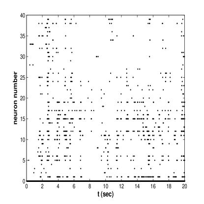
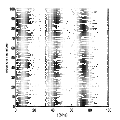
Figure 1: Example of spike trains from 40 salamander retinal ganglion cells (left panel) and 100 neurons in the cortical network model (right panel).

The strengths of the conductances were chosen so that, when firing, the network was in a high-conductance state, with effective membrane time constants around a millisecond, as described by Destexhe and coworkers [13]. There was no variation in the magnitudes of the synaptic conductances within a class (excitatory-excitatory, excitatory-inhibitory, etc.) beyond that implied by the random dilution, although there was random variation in their temporal characteristics.

A balanced state in this network requires very strong inhibitory synapses to balance the excitatory ones, which are four times more numerous in this network. The model we will use to fit the data (see below) does not have conductance-based synapses, so to gauge how much stronger the inhibitory synapses are, it is useful to compare effective current-based synaptic strengths, computed from conductances $g$ as $g(V_{rev}-\overline{V})$, where $V_{rev}$ is the reversal potential for the synapse (excitatory or inhibitory) and $\overline{V}$ is a typical value of the membrane potential in the balanced state. For this network, the ratio of the (absolute value of the) inhibitory effective couplings to the excitatory ones, estimated in this way, is about 4 for excitatory to inhibitory synapses and about 7 for excitatory-to-excitatory ones.

We collected spike data for 4350 seconds of simulated time and binned the spike trains using 10-ms bins. (Here, our choice of bin size was dictated by our prior knowledge of the range of the synaptic time constants in the model network.) The excitatory neurons had a mean firing rate of 8.77 Hz, and the inhibitory ones had a mean rate of 12.897 Hz. For the analysis, we used the 100 neurons with the highest firing rates. Of these, 66 were excitatory and 34 inhibitory. Their rates ranged from 24.46 Hz to 52.47 Hz, with a mean of 35.43 Hz. In the analysis, the data were treated as 128 25-second repetitions of a measurement.

For both data sets, having chosen the time bin size, the state of each neuron in each bin is characterized by a binary variable, $S_{i}(t)=\pm 1$ according to whether neuron $i$ fires or does not fire in time step (bin) $t$.

2.2 Kinetic Ising models

We are interested in inferring a statistical model that maximizes the probability of the spike histories $\{S_{i}(t)\}_{i=1}^{N}$, $1\leq t\leq T$. This is different from what one does for Gibbs equilibrium models [1, 6, 7], where one is concerned only with modeling the distribution of spike patterns, irrespective of their temporal order.

We consider a discrete-time kinetic Ising model. The state of each neuron is characterized by a binary variable, $S_{i}(t)=\pm 1$ according to whether neuron $i$ fires or does not fire in time step (bin) $t$. The dynamics of the model is defined by a simple stochastic update rule: At each time step, neurons receive inputs, $H_{i}(t)$, from both an external driving field $h_{i}(t)$ and the other neurons presynaptic to them:

$$H_{i}(t)=h_{i}(t)+\sum_{j}J_{ij}S_{j}(t).$$ (1)

Each neuron then, independently of all the others, fires at the next time step with a probability, conditional on the current neuron states, which is a logistic sigmoidal function of its total input:

$${\rm{Pr}}(S_{i}(t+1)=1|\{s_{j}(t)\})=f(H_{i}(t)),$$ (2)

where $f(x)=1/(1+\rme^{-2x})$. The parameters of this model are the external fields $h_{i}(t)$ and the couplings $J_{ij}$. For deriving the learning rules for $J_{ij}$ and $h_{i}(t)$, it will be convenient to write Eq.(2) in the form

$${\rm{Pr}}(S_{i}(t+1)|\{s_{j}(t)\})=\frac{\exp[S_{i}(t+1)H_{i}(t)]}{2\cosh H_{i}(t)}.$$ (3)

If $h_{i}(t)$ is time-dependent, the network statistics will be nonstationary. This gives us the possibility of describing nonstationary data, provided it is reasonable to assume that the $J_{ij}$ do not change in time. Of course, then we need data from many repetitions of the history of the network to be able to find the $h_{i}(t)$. It is important to keep in mind that the $h_{i}(t)$ represent more than just the external stimulus controlled by the experimenter. In addition to the external stimulus, they represent all the input to the recorded neurons from other neurons. It will not in general be possible to account for the correlations between these neurons in terms of the spatiotemporal variation of the stimulus, because they may interact with each other.

It will be useful to compare these models with independent-neuron ones, which are simply defined by (2) and (3) with all $J_{ij}=0$.

It is also possible to formulate an asynchronous-update version of the stationary model [14]. In this case, if the fields $h_{i}$ are constant in time and the $\sf J$ matrix is symmetric, the network relaxes to the stationary Gibbs distribution model of [1].

2.3 Objective function

We assume that the data consist of $R$ “trials” or repetitions of the network evolution, each of length $L$ time steps. Accordingly, we denote the state of neuron $i$ at time step $t$ in trial $r$ by $S_{i}(t,r)$. The objective function to be maximized in fitting the model parameters is the log-likelihood of the data $\{S_{i}(t,r)\}$ under the model,

$${\cal L}=\sum_{i=1}^{N}\sum_{r=1}^{R}\sum_{t=1}^{L}\{S_{i}(t+1,r)H_{i}(t,r)-\log[2\cosh H_{i}(t,r)]\},$$ (4)

where the $H_{i}(t,r)$ depend on the $S_{i}(t,r)$ in the same way as in Eq. (1) and $N$ is the number of neurons.

2.4 Exact algorithm

We find the $h_{i}(t)$ and $J_{ij}$ by gradient ascent on Eq. (4):

$$\delta h_{i}(t) = \frac{\eta}{L}\frac{\partial{\cal L}}{\partial h_{i}(t)}=\frac{\eta}{L}\langle S_{i}(t+1,r)-\tanh(H_{i}(t,r))\rangle_{r}$$ (5)

$$= \frac{\eta}{L}[m_{i}(t+1)-\langle\tanh(H_{i}(t,r))\rangle_{r}]$$

$$\delta J_{ij} = \frac{\eta}{L}\frac{\partial{\cal L}}{\partial J_{ij}}=\eta\langle[S_{i}(t+1,r)-\tanh(H_{i}(t,r))]S_{j}(t,r)\rangle_{r,t},$$ (6)

where $m_{i}(t)=\langle S_{i}(t,r)\rangle_{r}$ is the trial mean of $S_{i}(t,r)$ and $\eta$ is a learning rate. The averages are over the data – in (5) over repetitions for each time step $t$ and in (6) over both repetitions and time steps. We use the term “exact” to describe this algorithm in the sense that if the data were generated by this model, it would recover the parameters exactly in the limit $R\to\infty$ of infinite data.

The exact algorithm for the stationary model is very similar; the only difference is that we can regard each time step as a trial. Then the averages are only over time steps:

$$\delta h_{i} = \frac{\eta}{L}\frac{\partial{\cal L}}{\partial h_{i}}=\eta\langle S_{i}(t+1)-\tanh(H_{i}(t))\rangle_{t}$$

$$\delta J_{ij} = \frac{\eta}{L}\frac{\partial{\cal L}}{\partial J_{ij}}=\eta\langle[S_{i}(t+1)-\tanh(H_{i}(t))]S_{j}(t)\rangle_{t}.$$ (7)

It is worth noting that both these algorithms are generally much faster than that for the stationary Gibbs distribution model.

Choosing the learning rate required a little trial and error. We found that a learning rate $\eta=0.05$ was the largest value for which we reliably found monotonic decreases of our error measures. Typically, 1000 iterations were necessary to achieve stable errors. In the results presented here, all runs were 1000 iterations unless specified otherwise.

For all neurons, there were time bins with no spikes in any trial, and for some neurons there were bins with spikes in every trial. Naive inference in this case would lead to $|h_{i}(t)|=\infty$. In these cases, we reduced the empirical $|\langle S_{i}(t)\rangle|$ by hand from $1$ $0.999$ or, in some cases, to $0.99999$. These correspond to $|h_{i}(t)|\approx 4$ and $6$, respectively. The results and conclusions we draw from them below do not appear to be sensitive to this choice.

2.5 Smoothing

Our nonstationary models have many parameters (there are $NT$ $h$s), especially when we use very small time bins, so it can be useful to reduce the effective number of parameters by smoothing the inferred $h$s in time. We can do this by subtracting a penalty term

$${\cal K}=\mbox{$\frac{1}{2}$}\kappa\sum_{it}[h_{i}(t+1)-h_{i}(t)]^{2}$$ (8)

from $\cal L$. This leads to an extra term in $\delta h_{i}(t)$ proportional to $\kappa[h_{i}(t-1)-2h_{i}(t)+h_{i}(t+1)]$.

2.6 Mean field theories

Mean field theories provide faster algorithms for inferring network parameters than the exact learning rules described above. However, they are approximations. Therefore in this paper we apply both exact and mean-field algorithms and compare the resulting inferred couplings.

We employ two kinds of mean field theories. We call the simpler of these naive mean field theory [15]. One starts with the learning rule (6) for $J_{ij}$ at $\delta J_{ij}=0$ (i.e., after learning is finished), again writing $S_{i}(t,r)=m_{i}(t)+\delta S_{i}(t,r)$, and expanding the tanh to first order in $\delta S$. Then the naive mean field equations

$$m_{i}(t+1)=\tanh[h_{i}(t)+\sum_{j}J_{ij}m_{j}(t)],$$ (9)

permit elimination of the zeroth order term, and one is left with a set of linear matrix equations:

$$\langle D_{ij}(t)\rangle_{t}=\sum_{k}J_{ik}B_{kj}^{(i)},$$ (10)

where

$$B_{jk}^{(i)}=\langle(1-m_{i}^{2}(t+1))C_{jk}(t)\rangle_{t}.$$ (11)

Thus, for each neuron $i$, we obtain

$$J_{ij}=\sum_{k}\langle D_{ik}(t)\rangle_{t}[({\sf B}^{(i)})^{-1}]_{kj}.$$ (12)

Once the couplings are found in this way, equations (9) can then be solved for the $h_{i}(t)$, knowing the $m_{i}(t)$.

Naive mean field theory (henceforth abbreviated nMF) is exact in the limit of weak coupling strength and also for arbitrary coupling in a large, densely-connected system if the mean of the couplings is positive and their standard deviation is not large relative to the mean. In the opposite limit (standard deviation much larger than mean), fluctuations around the mean field become important, and there is no general simple solution. One strategy is to expand around the weak coupling limit [16], as was done by two of us [15, 17]. Here we take another route: There exists an exact solution for densely connected systems if the coupling matrix $\sf J$ is strongly asymmetric ($J_{ij}$ and $J_{ji}$ independently distributed) [18, 19]. This is a reasonable assumption for randomly-wired neuronal networks, since $J_{ij}$ and $J_{ji}$ represent different synapses. Following Mézard and Sakellariou, we abbreviate this full mean-field theory simply as MF.

In this case the internal fields acting on different units are independent Gaussian variables, and (9) are replaced by

$$m_{i}(t+1)=\int Dx\tanh(b_{i}(t)+x\sqrt{\Delta_{i}(t)}),$$ (13)

where

$$\int Dx(\cdots)\equiv\int\frac{dx}{\sqrt{2\pi}}{\rm e}^{-\mbox{$\frac{1}{2}$}x^{2}}(\cdots)$$ (14)

means integrate over a univariate Gaussian,

$$b_{i}(t)=h_{i}(t)+\sum_{j}J_{ij}m_{j}(t)$$ (15)

is the internal field from naive mean-field theory, and the internal field variance is

$$\Delta_{i}(t)=\sum_{j}J_{ij}^{2}(1-m_{j}^{2}(t)).$$ (16)

If we again write $S_{i}(t,r)=m_{i}(t)+\delta S_{i}(t,r)$ and expand the tanh to first order in $\delta S$, this time using (13) instead of (9), we are again led to an equation of the form (12), but now with

$$B_{jk}^{(i)}=\left\langle\int Dx[1-\tanh^{2}(b_{i}(t)+x\sqrt{\Delta_{i}(t)})]C_{jk}(t)\right\rangle_{t}.$$ (17)

This calculation has to be done iteratively. We start with an initial guess for the $J$s from nMF. From it we estimate the field variances $\Delta_{i}(t)$ using (16), and using these we solve (13) for the $b_{i}(t)$ by numerical iteration. This enables us to calculate the $B_{kl}^{(i)}$ from (17) and, from them, the $J$s using (12). We then use these $J$s to get a better estimate of the $\Delta_{i}(t)$ and repeat the calculations, leading to new $J$s, and iterate this procedure until the couplings converge. In practice this took 5-10 iterations of both the outer (successive estimates of the $J$s) and inner (successive estimates of the $b_{i}(t)$) iteration loops.

2.7 Error and quality-of-fit measures

There are a number of measures of the error or quality of fit. One is the objective function itself. We use it, in conjunction with an Akaike penalty, in model comparison. Akaike [11] showed that, under rather general conditions, the log-likelihood evaluated on the data is a biased (over)estimate of the true log-likelihood of a model and, furthermore, that this bias is just equal to the number of parameters $k$ in the model. Thus, the Akaike penalty we subtract from the empirical log-likelihood in doing model comparison is simply the number of parameters.

The use of a different penalty term has been proposed in the statistical literature by Schwarz [20]. He takes a Bayesian approach, according to which the likelihood of a model is proportional to the integral over its posterior distribution. Assuming a flat prior and expanding the log-likelihood around its maximum, the quadratic term is proportional to the sample size $n$ and the integral to be done is over a $k$-dimensional Gaussian. The result is proportional to $n^{k/2}$. Taking the log of this gives Schwarz’s penalty, $k\log\sqrt{n}$. For large sample size, it penalizes large models more strongly than Akaike’s does.

The merits of these criteria, commonly called AIC (Akaike information criterion) and BIC (Bayesian information criterion), and others related to them are still discussed in the statistical literature [21]. Here we generally use Akaike’s, but in one case we also employ Schwarz’s and compare the conclusions they lead to.

The objective function is extensive in the number of neurons and the length of the data set. When we report computed values here (with or without Akaike or Schwarz penalties), they are per neuron per time step. We use natural logarithms; dividing our numbers by $\log 2$ expresses them in bits.

For the data generated by the computational cortical network, we know which connections are actually present, so we can also evaluate the following measure of the accuracy with which the true connections are found by the model. Consider the inhibitory synapses. In the computational network as implemented here, the strengths of their conductances are always the same if they are nonzero. The differences in their temporal characteristics are beyond the scope of our simple memory-less Ising model, so we have to disregard them here. We would then hope that the algorithm would find about the same (negative) value for $J_{ij}$ when there is an inhibitory synapse from $j$ to $i$ and zero otherwise. However, because of finite data and model mismatch, the $J$s found which should be negative are actually spread around some mean value $-J_{0}$, with standard deviation $\sigma_{1}$, and those which should be zero are actually spread around zero with some standard deviation $\sigma_{0}$. We therefore adopt as a measure of the network reconstruction error the noise-signal ratio

$$\zeta=\frac{\sigma_{1}+\sigma_{0}}{J_{0}}.$$ (18)

2.8 Other statistics

For both data sets and both kinds of models, with and without couplings, we also consider two more simple statistics. The first is the estimated probability of different numbers of synchronous (i.e., within the same time bin) spikes. Defining

$$M(t,r)=\mbox{$\frac{1}{2}$}\sum_{i}[1+S_{i}(t,r)],$$ (19)

the estimated probability of $M$ synchronous spikes is

$$P(M)=\frac{1}{RT}\sum_{r,t}\delta_{M(t,r),M}.$$ (20)

To construct the other statistic, we compile a list of the number of times every observed spike pattern $S_{i}(t,r)$ occurs in the data. We then rank-order this list by the sizes of these counts and plot the counts against the rank (a so-called Zipf plot).

3 Results

3.1 Model comparison

Salamander retinal data

We analyzed the fit of the kinetic Ising model to the data set of 40 ganglion cells in a salamander retina. We calculated the log likelihoods for this data in the exact nonstationary algorithm for different data sets sizes. Fig. 2a shows log likelihoods, with and without Akaike penalties, for nonstationary models with and without $J$s. For these data, the model with couplings is only slightly better than the independent neuron model: Almost all the variation in the data could be accounted for by the time-dependent inferred fields $h_{i}(t)$. Although for small $R$ taking into account Akaike adjustment has a big influence on the value of the log-likelihood, it loses its importance when enough repeats are present.

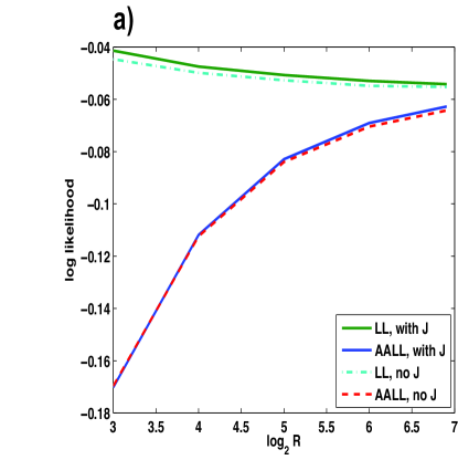
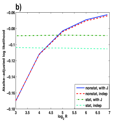
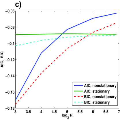
Figure 2: (a) Log likelihoods (per neuron, per bin) of retinal ganglion cell spike trains under nonstationary models with and without couplings, as functions of number of repetitions $R$ of the 26.5-s movie clip. The upper pair of curves are the raw log likelihoods, and the lower pair are the Akaike-corrected values. Within each pair, the higher curve is for the model with couplings and the lower is for an independent-neuron model. (b) Akaike-corrected log likelihoods under stationary and nonstationary models, with and without couplings. (c) Comparison of model comparisons (with couplings): AIC (solid lines) vs BIC (dashed lines).

This was not true for stationary models, as can be seen in Fig. 2b. Stationary models with $J$s are clearly always favored over those without, and for limited data (fewer than 28 repetitions) they are also favored over the nonstationary models.

Comparing the stationary and nonstationary models, the log-likelihood of the data under the stationary model is significantly less than the one under nonstationary model. One might argue that this is due to the fact that the nonstationary model without couplings has a lot more parameters than the stationary model with couplings. In fact this argument is correct when only a small number of repeats are used for inferring the nonstationary input: for small $R<28$ the nonstationary model performs worse than the stationary one when the Akaike penalty is taken into account. However, when there are enough repeats ($R>28$), the situation reverses: the nonstationary models, with or without couplings, outperform the stationary model with couplings even after Akaike corrections.

As mentioned above, Schwarz’s Bayesian approach penalizes models with many parameters (such as our nonstationary ones) more severely than Akaike’s. We therefore also applied the Schwarz penalty to the models with couplings. Fig. 2c shows both the Akaike and Schwarz stories: Under the Bayesian criterion, one needs data from at least 55 stimulus repetitions to conclude that the nonstationary model is superior, while under Akaike’s criterion only about half as many repetitions were necessary. However, the conclusion based on the entire data set available here (120 repetitions) is the same: the nonstationary model fits the data better.

The evident insignificance of the $J$s in the nonstationary model is also clarified by Fig. 3. Here we performed the inference (using the exact algorithm) separately for the first and second halves of the data and scattered the results $J$s against each other. Fig. 3 shows that almost all significant $J$s are inhibitory self-couplings, reflecting an apparent refractory tendency of the neurons. Couplings between neurons are small, and no systematic relation between those found from the two halves of the data is apparent.

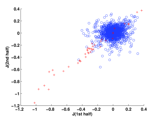
Figure 3: Couplings $J_{ij}$ inferred from salamander retinal data using a nonstationary model: Couplings inferrred from the first 60 repetitions of the stimulus movie clip plotted against those inferred from the second 60 repetitions. Blue circles indicate couplings between neurons ($J_{ij}$, $i\neq j$, and red crosses indicate self-couplings ($J_{ii}$).

We also inferred nonstationary models for the entire data set using smaller time bins: 2 and 10 ms. Since the number of $h$s in the model is inversely proportional to the bin size, we used the smoothing technique described in Sect. 2.5, adjusting the smoothing parameter $\kappa$ to keep the effective number of parameters approximately the same as for the 20-ms calculations without smoothing. Thus, the log likelihoods of these models could be compared directly with the 20-ms models and with each other (their Akaike penalties were approximately equal). We found that all of the models using smaller bins were inferior to the 20-ms model: The log likelihoods (per 20 ms) were $-0.124$, $-0.073$, and $-0.051$ for 2-, 10- and 20-ms bins, respectively. Increasing the size of the time bins, on the other hand, increases the likelihood. Eventually the log-likelihood converges to zero when the bin size encompasses the whole data set and the single bin is occupied. The model, however, is then a trivial one.

Nevertheless, the smaller-bin models revealed something interesting when we compared the $J$s inferred from the two halves of the data, as shown in the graphs in Fig. 4. They show that some credible $J$s, all positive, are inferred for the smaller time bins (2 and 5 ms). Perhaps these couplings are also present for larger time bins, but there they are lost inw the noise of the many spurious inferred $J$s. Comparison of the inferred $\sf J$ matrices and their transposes (not shown) revealed that these couplings are largely bidirectional. We note, however that, the presence of statistically significant Js for small bin sizes might also be a consequence of the regularization we imposed on the variation of the fields in order to limit model complexity. Indeed, for small bin sizes, the regularizer suppresses correlated fluctuations of fields at high frequency. High frequency correlated fluctuations in the spins can therefore be explained, within the regularized model, only by non-zero couplings.

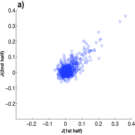
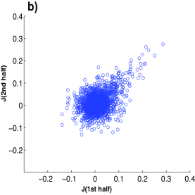
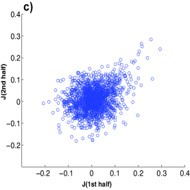
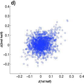
Figure 4: Off-diagonal couplings $J_{ij}$ inferred from the first 60 repetitions of the stimulus movie clip plotted against those inferred from the second 60 repetitions for salamander retinal data using nonstationary models based on (a) 2, (b) 5, (c) 10 and (d) 20 ms.

Returning to the 20-ms models, we also compared exact and mean-field algorithms on these data. One can see in Fig. 5a-c that nMF and MF agree qualitatively with the exact algorithm, except that they systematically overestimate large positive (and, to a lesser extent, large negative) $J$s. These differences appear to make very little difference in the estimates of the log likelihoods. For the exact algorithm, nMF, and MF, respectively, the log likelihoods (with the Akaike penalty) of the full nonstationary model on the complete data (120 repetitions) were -0.062748, -0.062872, and -0.062823. The differences are at most 0.2% or less, so all our conclusions above about model comparison can be drawn equally well from very fast (at most a few minutes) mean-field calculations as from the lengthy (several hours) calculations using the exact algorithm.

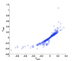
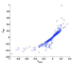
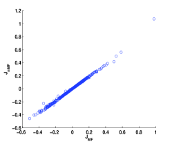
Figure 5: Comparison of couplings in nonstationary model inferred from retinal data by exact and mean field algorithms: exact algorithm vs nMF, exact algorithm vs MF, and nMF vs MF.

Model cortical network

We also investigated the fitting of our kinetic Ising model to data generated by our small cortical network model for which we could generate as much data as we wanted and for which the true connections and external field was known to us. Similar to the retinal data, as a quality-of-fit measure, we use the log-likelihood of the data under the kinetic Ising model. We do the analysis using the exact nonstationary algorithm for data sets of 8 up to 128 repetitions. Fig. 6a shows the log-likelihoods with and without the Akaike penalty as a function of the number of repetitions. The log-likelihoods are calculated with and without (independent-neuron model) the couplings $J_{ij}$. It is evident that the model with the $J$s is better than the one without them. In both cases, as the number of repetitions increases, the Akaike correction becomes less important. The same Akaike-adjusted log-likelihoods, with and without $J$s, are shown in Fig. 6b, together with the corresponding results for a stationary model. It is evident that the nonstationary independent model is much better than the stationary independent one for all numbers of repetitions. The quality of the nonstationary model with $J$s in comparison to the stationary one with $J$s depends on the number of repetitions. The nonstationary one has higher Akaike-adjusted log-likelihood when the number of repetitions is greater than 11. This shows that the size of the data set can be significant in the choice between models.

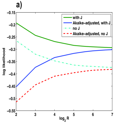
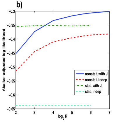
Figure 6: (a) Log likelihoods of the cortical model data as a function of number of stimulus repetitions under nonstationary models with and without couplings and with and without Akaike corrections. (b) Akaike-corrected log likelihoods, as functions of number of stimulus repetitions, under stationary and nonstationary models with and without couplings.

Next, we compare three different algorithms for the nonstationary model: exact, nMF, and MF. To visualize the comparisons, we make scatter plots. We plot the couplings obtained by each of three algorithms against each other, pairwise, in Figs. 7 a-c. The $J$s obtained by nMF and MF show nearly perfect agreement with each other; thus, for estimating the couplings, there is nothing to be gained from use the more time-consuming MF algorithm rather than the simpler nMF. Both mean-field algorithms give $J$s that generally agree quite well with those obtained by the exact algorithm, although they tend to overestimate $J$s when they are large and positive and, to a small degree, when they are large and negative.

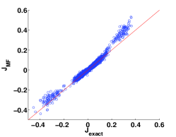
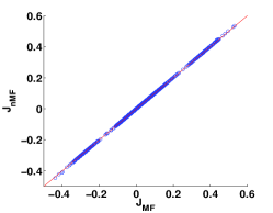
Figure 7: Comparison of couplings in nonstationary model inferred from cortical model data by exact and mean field algorithms: exact algorithm vs nMF, exact algorithm vs MF, and nMF vs MF.

As we did for the retinal data, we compared the mean-field approximations with the exact algorithm on these data. We found log likelihoods (with the Akaike penalty) for the nonstationary model with $J$s of -0.30307 for the exact algorithm, -0.30981 for nMF, and -0.30409 for MF. As was the case for retinal data, MF is closer to the exact result than nMF. However, the differences are around 2% or smaller, so again we conclude that all model comparisons of interest can be made using mean-field methods.

3.2 Network graph identification

The Akaike-penalized log likelihood is a suitable measure for comparing the quality of different models, but it is not necessarily informative for identification of the connections present in the network (i.e., the network graph). Of course, how well a model performs on this task is possible only when the true connections are known, which we do not in the case of the retinal data. We therefore examined histograms of the inferred $J$s for pairs of neurons that are connected and for pairs that are unconnected (Fig. 8a) in the cortical model. The strong inhibitory synapses are clearly identifiable as the peaks around $J\approx-0.3$.

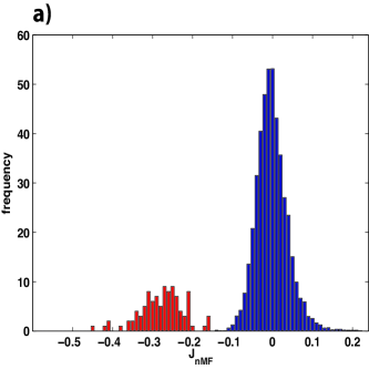
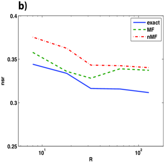
Figure 8: (a) Distributions of the couplings inferred from the cortical network data using the exact nonstationary algorithm. Red: inferred coupling values for neuron pairs for which an inhibitory synapse is present in the cortical model network. Blue: inferred coupling values for pairs with no connection in the cortical model network. (b) Noise/signal ratios $\zeta$ (Eq. 18), as functions of number of stimulus repetitions, for inhibitory couplings inferred from cortical model data using exact, nMF and MF algorithms.

There is not a qualitative difference between the exact and mean-field methods in how well they identify the inhibitory part of the network graph. However, there are quantitative differences. These are reflected in the values of the noise-signal ratio $\zeta$ defined in (18). Fig. 8b shows $\zeta$ as a function of data size (specifically, the number of repetitions), for the exact algorithm, nMF and MF. One can see that $\zeta$ does not depend strongly on the data size, but that MF is consistently somewhat better than nMF, though not as good as the exact result. We obtained similar results for this model in a tonic firing state using the stationary algorithm [22].

The much weaker excitatory synapses are not clearly identified by any of the algorithms. They are overshadowed by the large peak around zero, which mostly represents the far more numerous absent connections. This illustrates how identifying synapses in a network correctly by fitting a model such as this one depends on how strong they are.

3.3 Frequency of synchronous spikes and spike patterns

Fig. 9a shows the empirical distribution $P(M)$ (Eq. 20) of $M$ synchronous spikes for the retinal data, as calculated directly from the data and from two different models: a nonstationary independent-neuron model and a nonstationary model with couplings. Evidently, the observed distribution of synchronous spikes can be modeled very well without couplings provided that nonstationarity in the spike trains is taken into account, that is, by a nonstationary independent model. As would be expected from the likelihood comparison and lack of significance in the inferred couplings, adding couplings to the nonstationary independent model does not change how well $P(M)$ for these neurons is predicted by the model.

The situation is different for the cortical model data. Fig. 9b shows the probability of synchronous events calculated from the data and from the same two models. As would be anticipated from the log-likelihood measures, the nonstationary model without couplings cannot reproduce the pattern exhibited by the data, although it is far better than the stationary model without couplings (not shown). Adding couplings to the nonstationary model improves the quality of the fit, but the improvement is marginal. The fact that even the model with couplings cannot reproduce the shape of the empirical curve exactly indicates that one should improve the model, possibly by taking into account higher order correlations, or looking beyond one step in the past, to fully explain the data.

Fig. 9c shows that nonstationary models, with or without couplings, show an approximate power law behavior in a Zipf plot, very similar to that exhibited by the data. The two nonstationary models give nearly identical results (the two curves cannot be resolved in the plots) certainly as good or better than the Gibbs equilibium fit [9]

The nonstationary models also both do a good job of reproducing the Zipf plot in the cortical model data (Fig. 9d).

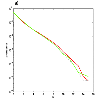
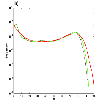
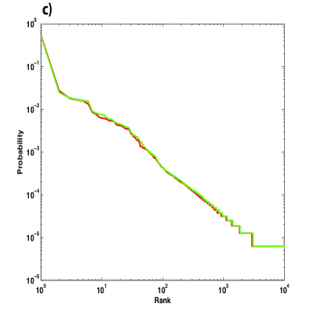
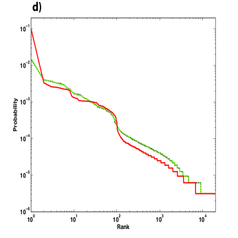
Figure 9: (a) The probability of M synchronous spikes occurring in 20-ms time bins, 40 salamander retinal ganglion cells. Red: calculated from data. Black: calculated from an independent nonstationary model. Green: calculated from a nonstationary model with couplings. (b) The same as (a) but for the cortical model data. (c) The probability of spike patterns from the 40 retinal ganglion cells as a function of their rank. (d) The same as (c) but for the cortical model data. (Colour coding in (b-d) as in (a).)

4 Discussion

In neuronal networks, correlations in the external input can influence the apparent correlations in firing of neurons. To understand neural information processing, it is thus important to distinguish between aspects of neural firing that are simply inherited from the external input and those that are generated by the network circuitry. This can be done by considering statistical models that allow for non-stationary external input and do not a priori assume stationary input. A simple example of such a model used in this paper is the kinetic Ising model that can be efficiently fitted to neural data and other point processes using exact and approximate inference methods.

The results reported in this paper show that it is possible, using the kinetic Ising model, to infer interactions from systems exposed to nonstationary external input. For the retinal data, we find that for stationary models the inclusion of couplings improves the fit qualitatively, as measured by the likelihood, but this is not the case for nonstationary models. Consistent with this, we also find that for nonstationary models the connection strengths inferred from one half of the data are very poorly predicted by those inferred from the other half. Of course, nonstationary models have more (for the present data, many more) parameters than stationary ones, so for limited data a stationary model may outperform the corresponding nonstationary one. However, for enough data, the log-likelihood of the nonstationary model, with or without couplings, becomes significantly larger than that of the stationary model even when the difference in the number of model parameters is corrected for. For the cortical model data, on the other hand,we find that the presence or absence of the couplings for both stationary and nonstationary models make a significant difference in the likelihood of the models. Furthermore, the inferred couplings using the nonstationary model are well correlated with the real synaptic connections in the network. In this case, again, the nonstationary model is significantly better than the stationary model.

For the retinal data, we explored using smaller time bins, ranging down to 2 ms. Nonstationary models inferred from such data appeared to give worse fits than those using 20-ms bins. However, interestingly, we found a few significant, positive, mostly bidirectional couplings for the smallest bins (2 and 5 ms). These couplings were not apparent in the 20-ms-bin-based models. They could be gap junctions or could represent the effect of synchronized common input from retinal interneurons not recorded from or included in the models.

For both the salamander retinal data and those from the local cortical network model, mean field methods were found to give nearly the same log likelihoods as those found using the exact algorithm. Since the mean field methods are at least a couple orders of magnitude faster than the exact calculations (which require up to 1000 iterations to converge for these data), this finding suggests that these methods may make it possible to explore, accurately and efficiently, model spaces much larger than ones that can be studied practically using the exact algorithm.

Our results on using the models to reproduce the observed probability of synchronous spikes largely parallel what we find by comparing the likelihoods. For the retinal data, the observed behavior can be perfectly described by a nonstationary external field, without requiring any couplings in the model. For the cortical data, on the other hand, the nonstationary input model alone without couplings cannot describe the pattern that the data shows for the frequency of synchronous spikes. Adding couplings in this case slightly helps but is not enough to explain the empirical results fully.

The empirical Zipf plots are also well described by the nonstationary independent model, but in this case adding the couplings does not seem to improve the capacity of the model to reproduce this feature. The emergence of Zipf’s law in the retinal data, has been interpreted as indicating criticality in the network [10] as indeed the corresponding stationary Ising models seem to be poised close to a critical point. Our results show that an alternative explanation is possible if nonstationarity is taken into account, in terms of non-interacting spins. In this picture, clearly, Zipf’s law has nothing to do with the retinal circuitry. Rather, it is a reflection of correlations in the statistics of the external input generated by the natural scene stimuli used in the experiment.

In their effort in modeling the same retinal data, Schneidman et al [1] compared the equilibrium Ising distribution fitted to the mean and pairwise (equal-time) correlations between neurons to the nonstationary model without couplings (which they call the conditionally independent model). They concluded that the equilibrium Ising distribution is more successful in modeling the data than the nonstationary model without couplings. However, their statement is based not on comparing log-likelihoods but on how much of the so called multi-information is captured by the models. Denoting the entropy of the spike patterns of $N$ neurons by $S_{N}$ and the entropy of an independent neuron fit to it by $S_{1}$, multi-information is defined as $I_{N}=S_{1}-S_{N}$. Denoting the entropy of an equilibrium Ising fit to the data by $S_{2}$ and that of a conditionally independent model by $S_{cond-int}$, Schneidman et al show that $I_{(2)}/I_{N}=(S_{2}-S_{N})/I_{N}$ is significantly larger than $I_{cond-ind}/I_{N}=(S_{con-int}-S_{N})/I_{N}$. For the equilibrium Ising model, $S_{2}$ is equal to the log-likelihood of the data under the model (what in this paper we use as our model quality measure) and $I_{(2)}$ is equal to the Kullback-Leibler divergence between the true distribution of spike patterns and the equilibrium Ising model fit to it. However, for the conditionally independent model this is not the case. It is therefore difficult to evaluate their statement in terms of log-likelihood. We have estimated the log likelihood (per neuron, per time bin) of the 20-ms-binned data under an equilibrium Ising model as $-0.0926$ (see A). (The Akaike penalty for this model, $(N+1)/2T\approx 10^{-4}$ is negligible.) This value is fairly close to what we found for the stationary model ($-0.0887$) and consequently also well below that for the nonstationary model (with or without couplings, $-0.0628$ and $-0.0643$, respectively).

The insignificance of the inferred connections in the retinal data does not mean that no couplings, statistical or physiological, exist between the cells. Instead, it means that the correlations, at the time scale and data length we had, do not reflect the effect of such connections and are better modeled by external input. In other words, the non-stationary model attributes correlated neuronal activity to correlations in the external input at 20ms. Little of the influence of direct interaction between neurons can be seen with the length of data available to us. Likewise, we are not in a position to draw definite conclusions on the significance of direct interactions detected for smaller bin sizes, since the regularization we had to impose suppresses fluctuations in the inputs over those frequencies. This issue could be resolved by longer recordings. However, the convergence of the Akaike-corrected and uncorrected log likelihoods in Fig. 2a shows that there is little room to improve corrected log likelihood by much: Most of the remaining failure to fit the data has to be blamed on the model. The kinetic Ising model is just a toy that we use here to illustrate the importance of nonstationary effects, but it lacks many features that a good neural model should have. The most obvious of these is the fact that neurons can integrate their synaptic inputs over longer periods than just one time step in our binned data. Generalized linear models (GLMs) [23, 24] include this feature in a general way. In fact, our kinetic Ising model is just a GLM without temporal integration kernels, and much of what we have done here can be extended straightforwardly to the general case. It also seems possible to improve the modeling of synapses and to take into account the large number of neurons in the network that are not recorded in the experiment.

However, even with better models, as we study larger and larger populations, longer and longer recordings will be required. An alternative (or parallel) approach to increasing the data length would then be to better exploit the available data by including terms in the objective function reflecting prior knowledge about the network connectivity or external input. For example, most recorded neurons are not connected to each other, so we are effectively trying to reconstruct a sparse network. In this case, L-1 regularization, in which the log likelihood is penalized by a term proportional to the sum of the absolute values of the $J$s, is a natural approach.

Pillow et al [24] analyzed monkey retinal neuronal data using a GLM. Unlike us, they found that the fit using a model with interactions between neurons was significantly better than that obtained without interactions. This could be a species difference. Alternatively, it might be because in the experiments which produced our data the stimulus was simply so strong as to dominate the firing statistics and mask interactions that might have been evident for weaker stimuli. There is also the difference between our model and theirs that they knew the stimulus and represented its effect through spatiotemporal inferred receptive fields, while we, not knowing it explicitly, represent its effect through the parameters $h_{i}(t)$. These parameters represent not only the stimulus itself, but also all trial-to-trial reproducible input to the recorded neurons from all the unrecorded neurons. In the model of Pillow et al, on the other hand, such correlated input is accounted for by couplings. Therefore it is difficult to compare their couplings with ours.

There is the further difference between the models that, although theirs used more parameters to describe the interactions than ours, it did not require a number of parameters that grew with the stimulus duration. It would be interesting to fit a model like theirs to data like those we have analyzed here, but for which the movie pixel intensities are known. This would allow us to determine to what degree the two species really differ in their retinal circuitry and to what degree the two experiments just differed in the strengths of their stimuli and/or the degree of correlated input to the recorded set of neurons.

Although we did not find that interactions improved the fit quality significantly, we did find an indication of a small number of significant effective couplings for 2- and 5-ms-bin data. In this respect, there is a qualitative agreement between our findings and those of Pillow et al. A more relevant comparison is with the findings of Cocco et al [5] on spontaneous salamander retinal ganglion cell data. Like us, they found significant positive, generally bidirectional couplings. However, our data on this timescale appear to be very noisy, so longer recordings would be needed to study these couplings satisfactorily.

We cannot say with certainty, on the basis of the data analyzed alone, what the biological meaning of the couplings inferred by any of the approaches discussed here is. The couplings found by Cocco et al and by us for small time bins almost certainly do not represent synapses. Rather, since they are positive and generally bidirectional, they could be either gap junctions, an effect of correlated common input from other kinds of cells in the retinal network, or external stimulus. It is not possible to distinguish these possibilities from the present spike data alone.

Our nonstationary model is able, by averaging over trials, to isolate effects due to reproducible correlated input from outside the recorded set of neurons, but it cannot do so if that input varies randomly from trial to trial. It ought to be possible to study such effects by including “hidden” neurons in the model and inferring connections to, from and among them in addition to those between neurons in the recorded population.

Appendix A Estimating the likelihood of the equilibrium Ising model

Denoting the partition function of an equilibrium Ising model by $Z_{\rm Ising}$ and the energy of a given configuration of spins, $\mathbf{s}$, by $E_{\rm Ising}(\mathbf{s})$, the log-likelihood of the data is

$${\cal L}_{\rm Ising}=\sum_{\mathbf{s}}E_{\rm Ising}(\mathbf{s})-L\log Z_{\rm Ising},$$ (21)

where $L$ is the number of samples. The difficult part in calculating this is estimating the partition function. We considered two ways of making this estimate, as described below.

Given an energy function $E_{\rm test}$ over the spin configuration, we have

$$Z_{\rm Ising}=Z_{\rm test}\sum_{\mathbf{s}}\frac{\exp(-E_{\rm test}(\mathbf{s}))}{Z_{\rm test}}\exp(-E_{\rm Ising}(\mathbf{s})+E_{\rm test}(\mathbf{s}))$$ (22)

$$\approx Z_{\rm test}\frac{1}{L}\sum^{L}_{l=1}\exp(-E_{\rm Ising}(\mathbf{s}^{l})+E_{\rm test}(\mathbf{s}^{l}))$$ (23)

where $\mathbf{s}^{l}$ are samples from the distribution with energy $E_{\rm test}$. Using this equation with a properly chosen $E_{\rm test}$ for which $Z_{\rm test}$ can be calculated easily thus allows estimating $Z_{\rm Ising}$ [25]. Taking $E_{\rm test}$ as an independent-neuron model with fields chosen to match the mean magnetizations of the data, we generated samples of length $L=4\times 10^{7}$ from this distribution and used them to estimate the Ising model partition function using the equation above.

We also generated samples from the Ising model itself using the Metropolis algorithm and considered the following estimate of the partition function:

$$Z_{\rm Ising}=\frac{1}{L}\sum^{L}_{l=1}\exp(-E_{\rm Ising}(\mathbf{s}^{l}))/p(\mathbf{s}^{l}),$$ (24)

where $p(\mathbf{s}^{l})$ is the experimental probability of observing $\mathbf{s}^{l}$ in the sequence generated from the metropolis algorithm. In this case, too, we used $L=4\times 10^{7}$ samples. Both estimators yielded a log likelihood per neuron per time step of $-0.0926$ for the retinal data set with 20-ms bins.

References

References

- [1] E. Schneidman, M.J. Berry, R. Segev, and W. Bialek. Weak pairwise correlations imply strongly correlated network states in a neural population. Nature, 440:1007–1012, 2006.
- [2] J. Shlens, G.D. Field, J.L. Gauthier, M.I. Grivich, D. Petrusca, A. Sher, A.M. Litke, and E.J. Chichilnisky. The structure of multi-neuron firing patterns in primate retina. J. Neurosci., 26:8254–8266, 2006.
- [3] T. R. Lezon, J. R. Banavar, M. Cieplak, A. Maritan, and N. Fedoroff. Using the principle of entropy maximization to infer genetic interaction networks from gene expression patterns. Proc. Natl. Acad. Sci. USA, 103, 2006.
- [4] S. Yu, D. Huang, W. Singer, and D. Nikolic. A Small World of Neuronal Synchrony. Cereb cortex, 18(12):2891–2901, 2008.
- [5] S. Cocco, S. Leibler, and R. Monasson. Neuronal couplings between retinal ganglion cells inferred by efficient inverse statistical physics methods. Proc. Natl. Acad. Sci. USA, 106:14058–62, 2009.
- [6] Y. Roudi, S. Nirenberg, and P. E. Latham. Pairwise maximum entropy models for studying large biological systems: when they can work and when they can’t. PLoS Comput Biol, 5:e1000380, 2009.
- [7] Y. Roudi, J. Tyrcha, and J. Hertz. Ising model for neural data: Model quality and approximate methods for extracting functional connectivity. Phys. Rev. E, 79(5):051915, 2009.
- [8] M. Weigt, R. A. White, H. Szurmant, J. A. Hoch, and T. Hwa. Identification of direct residue contacts in protein-protein interaction by message passing. PNAS, 106:67–72, 2009.
- [9] G. Tkacik, E. Schneidman, M. J. Berry II, and W Bialek. Spin glass models for a network of real neurons. arXiv:0912.5409v1 [q-bio.NC], 2009.
- [10] T. Mora and W. Bialek. Are biological systems posed at criticality? J Stat Phys., 144:268 302, 2011.
- [11] H. Akaike. A new look at the statistical model identification. IEEE Transactions on Automatic Control, 19:716–723, 1974.
- [12] John Hertz. Cross-Correlations in High-Conductance States of a Model Cortical Network. Neural Comp, 22(2):427–447, 2010.
- [13] A. Destexhe, M. Rudolph, and D. Pare. The high-conductance state of neocortical neurons in vivo. Nat Rev Neuro, 4(9):739–751, 2003.
- [14] H.-L. Zeng, E. Aurell, M. Alava, and H. Mahmoudi. Network inference using asynchronously updated kinetic ising model. Phys. Rev. E., 83:041135, 2011.
- [15] Y. Roudi and J. Hertz. Mean field theory for nonequilibrium network reconstruction. Phys. Rev. Lett., 106:048702, 2011.
- [16] T. Plefka. Convergence condition of the tap equation for the infinite-ranged ising spin glass model. J. Phys. A: Math. Gen., 15:1971–78, 1981.
- [17] Y. Roudi and J. Hertz. Dynamical TAP equations for non-equilibrium Ising spin glasses. J. Stat Mech: Theory and Exp., P03031, 2011.
- [18] M. Mezard and J. Sakellariou. Exact mean-field inference in asymmetric kinetic Ising systems. J. Stat. Mech.: Theory and Exp., L07001, 2011.
- [19] J. Sakellariou, Y. Roudi, M. Mezard, and J. Hertz. Effect of coupling asymmetry on mean-field solutions of direct and inverse sherrington-kirkpatrick model. Phil. Mag., 92:272–279, 2012.
- [20] G. E. Schwartz. Estimating the dimension of a model. Annals of Statistics, 6:461–464, 1978.
- [21] K.P. Burnham and D.R. Anderson. Model Selection and Multi-Model Inference: A Practical Information-Theoretic Approach. Springer, 2002.
- [22] J. A. Hertz, Y. Roudi, A. Thorning, J. Tyrcha, E. Aurell, and H-L. Zeng. Inferring network connectivity using kinetic ising models. BMC Neuroscience, 10, 2010.
- [23] W. Truccolo, U.T. Eden, M.R. Fellows, J.P. Donoghue, and E.N. Brown. A point process framework for relating neural spiking activity to spiking history, neural ensemble and extrinsic covariate effects. J. Neurophys., 93:1074–1089, 2005.
- [24] J. W. Pillow, J. Shlens, L. Paninski, A. Sher, A. M. Litke, E. J. Chichilnisky, and E. P. Simoncelli. Spatio-temporal correlations and visual signalling in a complete neuronal population. Nature, 454:995–999, 2008.
- [25] C. Bishop. Pattern Recognition and Machine Learning. Cambridge University Press, Cambridge, 2006.