We’ve walked a million miles for one of these smiles

Abstract

We derive a new, exact and transparent expansion for option smiles, which lends itself both to analytical approximation and to congenial numerical treatments. We show that the skew and the curvature of the smile can be computed as exotic options, for which the Hedged Monte Carlo method is particularly well suited. When applied to options on the S&P index, we find that the skew and the curvature of the smile are very poorly reproduced by the standard Edgeworth (cumulant) expansion. Most notably, the relation between the skew and the skewness is inverted at small and large vols, a feature that none of the models studied so far is able to reproduce. Furthermore, the around-the-money curvature of the smile is found to be very small, in stark contrast with the highly kurtic nature of the returns.

Understanding the shape of volatility smiles in option markets is arguably one of the most active field of research in quantitative finance Gatheral (2006); Fouque et al. (2000). By definition, the existence of an option smile is the sign that the standard Black-Scholes model is not an adequate representation of the stochastic dynamics of financial assets. A huge variety of models have been proposed over the years in order to account for the non-Gaussian nature of price changes and the corresponding option smiles: jumps and Lévy processes Cont and Tankov (2003), GARCH and stochastic volatility models Henry-Labordère (2010) (including the popular Heston and SABR models Hagan et al. (2002)), multiscale (multifractal) models Muzy et al. (2000); Bacry et al. (2001), mixed jumps/stochastic vol. models, etc. Another model-free strand of research that sheds light on the origin and the general structure of option smiles, is to assume that the corrections to the Black-Scholes model can somehow be considered as “small”. A natural idea is to use a Edgeworth cumulant expansion of the distribution of the price change $r_{T}=\frac{S_{T}-S_{0}}{S_{0}}$ (see Appendix). Working with the Bachelier model as benchmark (i.e. $(S_{t})_{t\geq 0}$ follows a Brownian motion instead of a Geometric Brownian motion), the authors of Bouchaud et al. (1998); Bouchaud and Potters (2003) have obtained the following cumulant expansion for the smile:

$$\sigma_{BS}=\sigma(1+\frac{\mathcal{S}_{T}}{6}\mathcal{M}+\frac{\kappa_{T}}{24}(\mathcal{M}^{2}-1)+\dots),\qquad\mathcal{M}:=\frac{K-S_{0}}{S_{0}\sigma\sqrt{T}}$$ (1)

where $\sigma\sqrt{T}$ denotes the standard deviation of $r_{T}$, $\mathcal{M}$ is the rescaled moneyness of the option, and $\mathcal{S}_{T}\ll 1$ and $\kappa_{T}\ll 1$ are respectively the skewness and kurtosis of $r_{T}$, which are assumed to be small for the expansion to make sense. Note that the authors of Backus et al. (1997) independently obtained a similar formula within a Black Scholes context, around the same time. The two formulas coincide for $\sigma\sqrt{T}\ll 1$, which is expected because in that limit the Black-Scholes model becomes identical to the Bachelier model.

The interest of the above formula is that it allows one to understand why smiles have generically an asymmetric parabolic shape, with an asymmetry related to the skewness of the distribution of the underlying, while the curvature of the smile is proportional to its kurtosis. Since from general arguments the distribution of $r_{T}$ becomes Gaussian at large times (albeit perhaps very slowly due to long-memory effects Bouchaud and Potters (2003)), the asymmetry and curvature of the smile are expected to go down with maturity $T$, as indeed observed in option markets.

However, the expansion (1) involves moments up to order $4$ and as such is troublesome both theoretically and practically. Indeed, the cumulative distribution of returns $P(|r_{T}|>x)$ is found empirically to decrease as $x^{-\mu}$ with $\mu\approx 3$ for many assets (see e.g. Plerou et al. (1999); Gopikrishnan et al. (1999)) and thus the moment of order $3$ is formally divergent. At any rate, it is in practice very difficult to estimate moments of order $3$ and $4$ because of the noise induced by large events. One possibility is to replace the skewness and kurtosis of $r_{T}$ by some lower moment approximations (cf. Bouchaud and Potters (2003)). However, this procedure is ambiguous as there is freedom in the choice of lower moments to be used.

The purpose of this note is to establish a different smile expansion formula, which is general, rigorous and involves no moments of order greater than $2$. This new smile formula lends itself to analytical treatments, which allow one to recover, for example, the recent results of Bergomi & Guyon Bergomi and Guyon (2011). But perhaps more importantly, our formula can be coupled to the “Hedged Monte-Carlo Method” of Bouchaud et al. (March 2001); Bouchaud et al. (2001a) to yield a powerful numerical method, which provides accurate estimates of the smile parameter for arbitrarily complex models of the underlying. One may even use historical data directly, short-circuiting any modelling assumption. Our formula, derived in the Appendix, reads:

$$\sigma_{BS}=\sigma(\alpha_{T}+\beta_{T}\mathcal{M}+\gamma_{T}\mathcal{M}^{2}+O(\mathcal{M}^{3})),$$ (2)

with the coefficients $\alpha_{T},\beta_{T},\gamma_{T}$ given by:

$$\alpha_{T}=\sqrt{\frac{\pi}{2}}E[|u_{T}|],\quad\beta_{T}=\sqrt{\frac{\pi}{2}}\left[1-2P(u_{T}>0)\right],\quad\gamma_{T}=\sqrt{\frac{\pi}{2}}\,p_{T}(0)-\frac{1}{2\alpha_{T}},$$ (3)

where $u_{T}=r_{T}/\sigma\sqrt{T}$ and $p_{T}(.)$ is the density of $u_{T}$. Using a Edgeworth expansion, one can show that both smile formulae (1) and (2) coincide in the limit where cumulants are small and cumulants higher than four can be neglected (see Appendix). One finds in particular $\beta_{T}\approx\mathcal{S}_{T}/6$. But what is remarkable is that while the “old” smile formula (1) is highly sensitive to extreme events, the new formula (2) only involves low moments of the distribution of $u_{T}$. In particular, the skew of the smile, as measured by the coefficient $\beta_{T}$, is technically a moment of order $0$, i.e. the large events do not play any role at all.

This new smile formula can be used in different ways. One can for example obtain directly the coefficients $\alpha_{T},\beta_{T},\gamma_{T}$ in a vol-of-vol expansion, recovering the Bergomi-Guyon results to lowest order Vargas (2012). One of the salient results of Bergomi & Guyon Bergomi and Guyon (2011) is that to leading order in vol-of-vol and for a broad family of linear models, the Edgeworth expansion result $\beta_{T}=\mathcal{S}_{T}/6$ holds, i.e. the skew of the smile $\beta$, and the skewness $\mathcal{S}_{T}$ of the distribution of $u_{T}$, are very simply related. A first exercise is to use our formula to investigate the case where the correlation between stock returns and volatility is non-linear. Assume for example a stochastic volatility model where $r_{T}=\int_{0}^{T}\sigma_{t}dW_{t}$, with $dW_{t}$ the standard Wiener process, and where the instantaneous volatility $\sigma_{t}^{2}$ is given by:

$$\sigma_{t}^{2}=\overline{\sigma}^{2}\left[1+2\epsilon(|\xi_{t}+\theta|\,1_{\xi_{t}+\theta<0})\right],\qquad\xi_{t}=\omega\int_{0}^{t}e^{-\omega(t-u)}dW_{u},\quad\epsilon>0.$$ (4)

Here $\overline{\sigma}^{2}$ is a “baseline” volatility (which might itself evolve over long times scales, see below).

When the threshold $\theta$ is zero, the above equation means that when recent returns are negative, the future volatility will be higher than usual (this is the standard leverage effect Bouchaud et al. (2001b); Bouchaud and Potters (2003)), while when the recent returns are positive, there is no impact on the future vol. When $\theta>0$, only relatively large negative returns will increase the volatility, while even small positive returns increase the volatility when $\theta<0$. The coefficients $\beta_{T}$ and $\mathcal{S}_{T}$ can be computed to first order in $\epsilon$ in this case Vargas (2012). One finds that the equality $\beta_{T}=\mathcal{S}_{T}/6$ only holds when $\theta=0$. When $\theta>0$, one the other hand, the skew amplitude $|\beta_{T}|$ is smaller than $|\mathcal{S}_{T}|/6$, and vice-versa when $\theta<0$. This shows that even for small vol-of-vols, non linear effects can significantly affect the relation between skew and skewness, and that there can be no general link between the two.

Although analytical results are interesting, we believe that the true added-value of our new smile expansion comes from the following remark: the three coefficents $\alpha_{T},\beta_{T}$ and $\gamma_{T}$ can be interpreted as the average payoff of some “exotic” options. Indeed, $\alpha_{T}$ is simply an at-the-money straddle, $\beta_{T}$ is related to an at-the-money binary option, and the first term of $\gamma_{T}$ is a “no move” option which pays if the underlying ends very close to its initial price. Having interpreted these coefficients as option prices, one can use the “Hedged Monte-Carlo” (HMC) method proposed in Bouchaud et al. (March 2001); Bouchaud et al. (2001a) to price these options numerically. This is interesting for at least two reasons (see Bouchaud et al. (March 2001); Bouchaud et al. (2001a); Bouchaud and Potters (2003); Petrelli et al. (2010) for a more thorough discussion): first, the HMC has by construction a low variance, that allows one to price options accurately with a relatively small number of paths; second, the P&L of the hedge automatically transforms historical or empirical probabilities into risk-neutral ones. Technically, the pricing of the “exotic” options is done in a way very similar to what is described in Bouchaud et al. (March 2001); Bouchaud et al. (2001a), except that we do not try here to determine the optimal hedge for these options, but rather use a (sub-optimal) Black-Scholes hedge. This reduces HMC to a standard reduced-variance Monte-Carlo Clewlow and Stricklands (1997) which is conceptually much simpler and faster numerically. Although only approximate, this pruned down version of HMC is accurate enough for the present purpose. The other subtle point concerns the pricing of the “no move” option, since one has to introduce a window with a small but finite width $\delta$, and carefully extrapolate the results to $\delta=0$. We in fact use a Gaussian payoff function, $\exp(-u_{T}^{2}/2\delta^{2})/\sqrt{2\pi\delta^{2}}$ for that purpose. We have calibrated the method on known cases – for example on the above non-linear model, with good agreement between the analytical calculations and the HMC results.

We now apply our method to real time series, using historical trajectories to price our exotic options and determine directly the skew $\beta_{T}$ and curvature $\gamma_{T}$ of the smile, without any a priori model. The data we use is the time series of daily returns (open-high-low-close) of the S&P500 index in the period 1/1/1970 – 31/12/2011. We divide the sample into two bins: one corresponding to high volatilities (larger than the median), the other to low volatilities, where the volatility is a 20 day exponential moving average of a Rogers-Satchell estimator of the squared daily volatility before the day the smile coefficients are determined. We show in Fig. 1 the “fair” skew $\beta_{T}$ as a function of $T$ for options between 1 and 20 days, that we compare with the prediction $\mathcal{S}_{T}/6$ based on a direct measure of the third moment skewness of the distribution of $u_{T}$. We find, perhaps surprisingly, that while $|\mathcal{S}_{T}|/6$ is systematically larger than the skew $|\beta_{T}|$ for large volatilities, the opposite is true for low volatilities. Let us emphasize here that we are not speaking of implied volatility smiles from option markets, but rather of theoretical predictions of what the fair parameters of the smile should be. Including some information from option markets could be done along the lines of Avellaneda et al. (2001).

In Fig. 2, we show the smile curvature $\gamma_{T}$ as a function of $T$ for the same two volatility regimes above, and compare it to $\kappa_{T}/24$, the curvature obtained from the Edgeworth expansion (1). Here again the results are surprising: we find that the “fair” curvature $\gamma_{T}$ of the smile around the money is close to zero, both for high and low volatilities. This is very different from what the empirical kurtosis of the distribution suggests, especially in the high vol regime where the kurtosis of returns is empirically very substantial, in agreement with the fact, noted above, that the distribution of returns exhibits power-law tails. This is a striking illustration of the misleading character of the Edgeworth expansion (1): the around-the-money smile of index options should be close to a straight line with very little curvature, as indeed often seen on implied smiles, whereas the Edgeworth expansion would predict highly curved smiles.

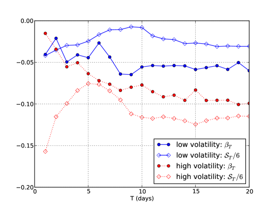
Figure 1: S&P500 data. Skew $\beta_{T}$ and skewness $\mathcal{S}_{T}/6$ for different volatility regimes. Note the inversion of the order between the two quantities as the volatility increases.

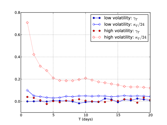
Figure 2: S&P500 data. Curvature $\gamma_{T}$ and kurtosis $\kappa_{T}/24$ for different volatility regimes. Note that, surprisingly, the curvature of the smile is found to be very small in both volatility regimes.

The results on the skew of the smile shown in Fig. 1 are clearly inconsistent with the relation $\beta_{T}=\mathcal{S}_{T}/6$, and cannot be understood either within the above non-linear leverage effect with a fixed parameter $\theta$. A way out would be to assume that $\theta$ itself depends on the “baseline” volatility $\overline{\sigma}$ in Eq. (4) above, with $\theta>0$ during high volatility periods and $\theta<0$ during low volatility periods. This could be interpreted as meaning that at high vols, a significant down-trend is required to drive the volatility even higher, whereas at low vols, it takes a moderate down-trend to move the volatility up. It is also instructive to compare these results with the predictions of a popular asymmetric GARCH model used to model the dynamics of the S&P500 index Berd (2011). Writing the returs as $\sigma_{t}\eta_{t}$ with $\eta_{t}\sim{\mathcal{N}}(0,1)$, the dynamics of $\sigma_{t}$ is postulated to be:

$$\sigma_{t}=\sigma(1+\chi_{t});\qquad\chi_{t+1}=\rho\chi_{t}+\nu(1+\chi_{t})\left[\eta_{t}^{2}1_{\eta_{t}<0}-\frac{1}{2}\right].$$ (5)

We have run our HMC on synthetic time series generated using the asymmetric GARCH (GAARCH) model with parameters $\rho=0.9$ and $\nu=0.1$, corresponding to a “memory time” of the volatility equal to 10 days. One can of course now generate as many trajectories as needed to get good statistics. The results for $\beta_{T}$ and $\gamma_{T}$ together with their corresponding cumulant expansion expressions are reported in Fig. 3 for the high volatility regime. We observe in this case a trend similar to the S&P500 data: the skewness $|\mathcal{S}_{T}|/6$ exceeds $|\beta_{T}|$ in absolute value and $\kappa_{T}/24$ is systematically larger than $\gamma_{T}$, although the latter is significantly different from zero. However, for low volatilities (not shown) the behavior of the skew is qualitativaly different from the S&P500 data. In that case $\beta_{T}$ and $\mathcal{S}_{T}/6$ are very close (except for very small T), but with still $|\mathcal{S}_{T}|/6>|\beta_{T}|$. In other words, the inversion observed on empirical data for low vols cannot be reproduced within the GAARCH model. That $|\mathcal{S}_{T}|/6>|\beta_{T}|$ can in fact be checked analytically in a small $\nu$ expansion. Note this inequality implies that the “Skew Stickiness Ratio” introduced by Bergomi in Bergomi (December 2009) is expected to be smaller than 2 at small maturities.

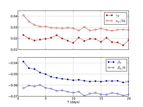
Figure 3: GAARCH synthetic data from equation (5), with $\rho=0.9$, $\nu=0.1$, and $10^{6}$ Monte Carlo paths for high volatility regime. Upper panel: curvature $\gamma_{T}$ and kurtosis $\kappa_{T}/24$. Lower panel: skew $\beta_{T}$ and skewness $\mathcal{S}_{T}/6$.

As a conclusion, we have set up a new, exact and transparent expansion for option smiles, which lends itself both to analytical approximation and, perhaps more importantly, to congenial numerical treatments. We have shown that the skew and the curvature of the smile can be computed as exotic options, for which the Hedged Monte Carlo method is particularly well suited. When applied to options on the S&P index, we have found that the skew and the curvature of the smile are very poorly reproduced by the standard Edgeworth (cumulant) expansion, or by the Bergomi-Guyon vol-of-vol expansion (at least to lowest order). Most notably, the relation between the skew and the skewness is inverted at small and large vols, a feature that none of the models studied so far is able to reproduce. We have argued that some coupling between the leverage effect and the volatility level is needed to capture such non-trivial statistical features. Finally, the around-the-money curvature of the smile is found to be very small, in stark contrast with the highly kurtic nature of the returns. This would also require some more detailed understanding. We hope that the ideas and methods presented in this paper are of general interest, and provide a fruitful framework to interpret the information provided by option markets.

We thank Marc Potters and Arthur Berd for many stimulating discussions. We are indebted to Julien Meltz who was involved in the earlier stages of this project. Finally, we thank L. Bergomi, J. Guyon, J. Gatheral and V. Kapoor for useful comments on the manuscript.

Technical Appendix

Proof of the smile formula

We denote the price $S_{T}=S_{0}(1+r_{T})$. We suppose that $r_{T}$ is centered and that $\sigma^{2}T=E[r_{T}^{2}]$. We set $u_{T}=r_{T}/\sigma\sqrt{T}$. We have:

$$E[(S_{T}-K)_{+}] =S_{0}E[(r_{T}-(\frac{K}{S_{0}}-1))_{+}]=S_{0}\int_{\frac{K-S_{0}}{S_{0}}}^{\infty}P(r_{T}>x)dx$$

$$=S_{0}\sigma\sqrt{T}\int_{\mathcal{M}}^{\infty}P(u_{T}>u)du$$

where we introduce the renormalized moneyness $\mathcal{M}=\frac{K-S_{0}}{\sigma\sqrt{T}S_{0}}$. A direct expansion in $\mathcal{M}$ leads to:

$$E[(S_{T}-K)_{+}]\approx S_{0}\sigma\sqrt{T}(\frac{E[|u_{T}|]}{2}-\mathcal{M}P(u_{T}>0)+\frac{\mathcal{M}^{2}}{2}p_{T}(0))$$

In the Gaussian case, we get therefore:

$$E[(S_{T}-K)_{+}]\approx S_{0}\sigma_{BS}\sqrt{T}(\frac{1}{\sqrt{2\pi}}-\frac{\mathcal{M}_{G}}{2}+\frac{\mathcal{M}_{G}^{2}}{2}\frac{1}{\sqrt{2\pi}})$$

where $\mathcal{M}_{G}=\frac{K-S_{0}}{\sigma_{BS}\sqrt{T}S_{0}}$ is the Gaussian moneyness.

We make now make the assumption:

$$\sigma_{BS}=\sigma(\alpha^{\prime}+\beta^{\prime}\mathcal{M}_{G}+\gamma^{\prime}\mathcal{M}_{G}^{2}),$$ (6)

so by definition $\mathcal{M}=\mathcal{M}_{G}(\alpha^{\prime}+\beta^{\prime}\mathcal{M}_{G}+\gamma^{\prime}\mathcal{M}_{G}^{2})$. The smile formula corresponds to the following identity:

$$\sigma_{BS}(\frac{1}{\sqrt{2\pi}}-\frac{\mathcal{M}_{G}}{2}+\frac{\mathcal{M}_{G}^{2}}{2}\frac{1}{\sqrt{2\pi}})=\sigma(\frac{E[|u_{T}|]}{2}-\mathcal{M}P(u_{T}>0)+\frac{\mathcal{M}^{2}}{2}p_{T}(0))$$

Therefore, we get the following equation (to the order $\mathcal{M}_{G}^{2}$):

$$(\alpha^{\prime}+\beta^{\prime}\mathcal{M}_{G}+\gamma^{\prime}\mathcal{M}_{G}^{2})(\frac{1}{\sqrt{2\pi}}-\frac{\mathcal{M}_{G}}{2}+\frac{\mathcal{M}_{G}^{2}}{2}\frac{1}{\sqrt{2\pi}})=(\frac{E[|u_{T}|]}{2}-(\alpha^{\prime}\mathcal{M}_{G}+\beta^{\prime}\mathcal{M}_{G}^{2})P(u_{T}>0)+\frac{\alpha^{\prime 2}\mathcal{M}_{G}^{2}}{2}p_{T}(0)).$$

which finally lead to the following identification:

$$\left\{\begin{array}[]{l}\alpha^{\prime}=\sqrt{\frac{\pi}{2}}E[|u_{T}|]\\ \beta^{\prime}=\pi E[|u_{T}|](\frac{1}{2}-P(u_{T}>0))\\ \gamma^{\prime}=\sqrt{2\pi}(\frac{\alpha^{\prime 2}p_{T}(0)}{2}-\frac{\alpha^{\prime}}{2\sqrt{2\pi}}+\pi E[|u_{T}|](\frac{1}{2}-P(u_{T}>0))^{2})\\ \end{array}\right.$$

Switching back to standard moneyness and using $\sigma_{BS}=\sigma(\alpha+\beta\mathcal{M}+\gamma\mathcal{M}^{2})$ finally leads to:

$$\left\{\begin{array}[]{l}\alpha=\sqrt{\frac{\pi}{2}}E[|u_{t}|]\\ \beta=\frac{\beta^{\prime}}{\alpha}=\sqrt{2\pi}(\frac{1}{2}-P(u_{t}>0))\\ \gamma=\frac{\gamma^{\prime}}{\alpha^{2}}-\frac{\beta^{\prime 2}}{\alpha^{3}}=\sqrt{2\pi}(\frac{p_{T}(0)}{2}-\frac{1}{2\alpha\sqrt{2\pi}})\\ \end{array}\right.$$

The Edgeworth expansion

Assuming $\mathcal{S}_{T},\kappa_{T}\ll 1$, the Edgeworth expansion reads:

$$P(\frac{r_{T}}{\sigma\sqrt{T}}>x)-\overline{N}(x)\approx\frac{\mathcal{S}}{6}N^{(3)}(x)-\frac{\kappa}{24}N^{(4)}(x).$$

where $N(x)=\int_{-\infty}^{x}\frac{e^{-t^{2}/2}}{\sqrt{2\pi}}dt$, $\overline{N}=1-N$ and $N^{(n)}$ refers to the $n$th derivative of $N$. This leads to the following approximations:

$$\left\{\begin{array}[]{l}\alpha\approx 1-\frac{\kappa_{T}}{24}\\ \frac{1}{2}-P(u_{T}>0)\approx-M_{T}p_{T}(0)\approx-\frac{M_{T}}{\sqrt{2\pi}}\ll 1\\ p_{T}(0)-\frac{1}{\sqrt{2\pi}}\approx\frac{1}{\sqrt{2\pi}}\frac{\kappa_{T}}{8}\ll 1\\ \end{array}\right.$$

where $M_{T}$ is the median of $u_{T}$. With these assumptions, we get the following expressions for $\alpha,\beta,\gamma$:

$$\left\{\begin{array}[]{l}\alpha\approx 1-\frac{\kappa_{T}}{24}\\ \beta\approx-M_{T}\\ \gamma\approx\frac{\sqrt{2\pi}}{2}(\frac{1}{\sqrt{2\pi}}(1+\frac{\kappa_{T}}{8})-\frac{1}{\sqrt{2\pi}}(1+\frac{\kappa_{T}}{24}))\approx\frac{\kappa_{T}}{24}\\ \end{array}\right.$$

Within the aforementioned approximation, both smile formulas coincide since we know that the Edgeworth expansion also leads to:

$$\mathcal{S}_{T}\approx-6M_{T},\quad\kappa_{T}\approx 24(1-\sqrt{\frac{\pi}{2}}E[|u_{T}|])$$

References

- Gatheral (2006) J. Gatheral, The Volatility Surface: A Practitioner’s Guide (Wiley Finance, 2006).
- Fouque et al. (2000) J.-P. Fouque, G. Papanicolaou, and R. Sircar, Derivatives in Financial Markets with Stochastic Volatility (Cambridge University Press, 2000).
- Cont and Tankov (2003) R. Cont and P. Tankov, Financial Modelling with Jump Processes (Chapman & Hall / CRC Press, 2003).
- Henry-Labordère (2010) P. Henry-Labordère, Analysis, Geometry, and Modeling in Finance: Advanced Methods in Option Pricing (Chapman & Hall / CRC Press, 2010).
- Hagan et al. (2002) P. Hagan, D. Kumar, A. Lesniewski, and D. Woodward, Wilmott magazine pp. 84–108 (2002).
- Muzy et al. (2000) J.-F. Muzy, J. Delour, and E. Bacry, Eur. Phys. J. B 17, 537 (2000).
- Bacry et al. (2001) E. Bacry, J. Delour, and J.-F. Muzy, Phys. Rev. E 64, 026103 (2001).
- Bouchaud et al. (1998) J.-P. Bouchaud, R. Cont, and M. Potters, Europhysics Letters 41, 239 (1998), first version on arXiv/9609172 (1996).
- Bouchaud and Potters (2003) J.-P. Bouchaud and M. Potters, Theory of Financial Risk and Derivative Pricing (Cambridge University Press, 2003).
- Backus et al. (1997) D. Backus, S. Foresi, K. Lai, and L. Wu, Working paper of NYU Stern school of Business (1997).
- Plerou et al. (1999) V. Plerou, P. Gopikrishnan, L. Amaral, M. Meyer, and H. Stanley, Phys. Rev. E 60, 6519 (1999).
- Gopikrishnan et al. (1999) P. Gopikrishnan, V. Plerou, L. Amaral, M. Meyer, and H. Stanley, Phys. Rev. E 60, 5305 (1999).
- Bergomi and Guyon (2011) L. Bergomi and J. Guyon (2011), http://ssrn.com/abstract=1967470.
- Bouchaud et al. (March 2001) J.-P. Bouchaud, M. Potters, and D. Sestovic, Risk Magazine pp. 133–136 (March 2001).
- Bouchaud et al. (2001a) J.-P. Bouchaud, M. Potters, and D. Sestovic, Physica A 289, 517 (2001a).
- Vargas (2012) V. Vargas (2012), in preparation.
- Bouchaud et al. (2001b) J.-P. Bouchaud, A. Matacz, and M. Potters, Phys. Rev. Lett. 87, 228701 (2001b).
- Petrelli et al. (2010) A. Petrelli, R. Balachandran, O. Siu, R. Chatterjee, Z. Jun, and V. Kapoor (2010), http://ssrn.com/abstract=1530046.
- Clewlow and Stricklands (1997) L. Clewlow and C. Stricklands, The Journal of Fixed Income 7, 35 (1997).
- Avellaneda et al. (2001) M. Avellaneda, R. Buff, C. Friedman, N. Grandechamp, L. Kruk, and J. Newman, International Journal of Theoretical and Applied Finance 4, 91 (2001).
- Berd (2011) A. Berd (2011), arXiv:1112.1114v1[q-fin.PM].
- Bergomi (December 2009) L. Bergomi, Risk Magazine pp. 94–100 (December 2009).