STUDY OF THE $\mathrm{\displaystyle}\eta\rightarrow e^{+}e^{-}\gamma$ DECAY USING WASA-at-COSY DETECTOR SYSTEM

Dla Moich Rodziców

Introduction

The term meson stems from the Greek word mesos which means middle. It was used by Hideki Yukawa to name a particle with a mass between the mass of an electron and a proton. At present, under this term, strongly interacting hadrons with a baryon number equal to zero are included.

The elementary components of mesons are quarks and antiquarks: fermions with baryon number $\mathrm{\pm}\nicefrac{{1}}{{3}}$. In the lowest energy state of quark-antiquark pairs, where the spins are anti-parallel, they create a pseudoscalar meson of negative parity and zero orbital angular momentum. Nine of these mesons, having spin equal to zero, form the pseudoscalar nonet, a member of which is the $\mathrm{\displaystyle}\eta$ meson.

The $\mathrm{\displaystyle}\eta$ meson was discovered in the 1960s at the Berkeley Bevatron [1] in the $\mathrm{\pi^{+}d\rightarrow pp\pi^{+}\pi^{-}\pi^{0}}$ reaction. Since then, many efforts have been made to investigate and understand its inner properties. Experimentally, the mass of this meson was found to be $\mathrm{547.853\pm 0.024\,MeV}$ [2]. In terms of the SU(3)-flavour group, the $\mathrm{\displaystyle}\eta$ meson can be represented as the superposition of the singlet $\mathrm{\eta}_{1}$ and the octet $\mathrm{\eta}_{8}$ state characterized by the mixing angle $\mathrm{\theta}$

$$|\eta\rangle=cos\theta|\eta_{8}\rangle-sin\theta|\eta_{1}\rangle,$$ (1)

where

$$|\eta_{1}\rangle=1/\sqrt{3}(u\bar{u}+d\bar{d}+s\bar{s})\quad\mbox{and}\quad|\eta_{8}\rangle=1/\sqrt{6}(u\bar{u}+d\bar{d}-2s\bar{s}).$$ (2)

Unlike the octet state, the singlet state can be either a quark-antiquark combination or a pure gluon configuration. In order to describe the $\mathrm{\displaystyle}\eta$ mass, both, the mixing and the dynamics of gluons have to be taken into account [5, 6, 7].

For the $\mathrm{\displaystyle}\eta$ meson is a short-lived, neutral particle, it is not possible to investigate its structure via the classical method of particle scattering. To learn about its quark wave function, one studies those decay processes of this meson, in which a pair of photons is produced, at least one of them being virtual. The virtual photons have a non-zero mass and convert into lepton-antilepton pairs. The squared four-momentum transferred by the virtual photon corresponds to the squared invariant mass of the created lepton-antilepton pair. Therefore, information about the quarks’ spatial distribution inside the meson can be achieved from the lepton-antilepton invariant mass distributions by comparison of empirical results with predictions, based on the assumption that the meson is a point-like particle. The last can be obtained from the theory of Quantum Electrodynamics. The deviation from the expected behavior in the leptonic mass spectrum expose the inner structure of the meson. This deviation is characterized by a form factor. It is currently not possible to precisely predict the dependence of the form factor on the four-momentum transferred by the virtual photon in the framework of Quantum Chromodynamics theory. Therefore, to conduct calculations, assumptions about the dynamics of the investigated decay are needed.

The knowledge of the form factors is also important in studies of the muon anomalous magnetic moment, $\mathrm{a_{\mu}=(g_{\mu}-2)/2}$, which is the most precise test of the Standard Model and, as well, may be an excellent probe of new physics. The theoretical error of calculation of $\mathrm{a}_{\mu}$ is dominated by hadronic corrections and therefore limited by the accuracy of their determination. Especially, the hadronic light-by-light scattering contribution to $\mathrm{a}_{\mu}$ includes two meson-photon-photon vertices and therefore also depends on the form factors [8]. At present, the discrepancy between the $\mathrm{a}_{\mu}$ prediction based on the Standard Model and its experimental value [9] is equal to $\mathrm{(28.7\pm 8.0)\cdot 10^{-10}}$ ($\mathrm{3}.6\sigma$) [10].

The goal of this work is to extract the electromagnetic transition form factor for the $\mathrm{\displaystyle}\eta$ meson through the study of its decay to the $\mathrm{\displaystyle}e^{+}e^{-}\gamma$ final state. For this aim the $\mathrm{\displaystyle}\eta$ mesons were produced in proton-deuteron collisions in the $\mathrm{\displaystyle}pd\rightarrow{}^{3}He\,\eta$ reaction. The measurement was performed using the WASA[11] detector system and the proton beam of the Cooler Synchrotron COSY [12]. The $\mathrm{4}\pi$ geometry of the WASA-at-COSY detector and its availability to work with high luminosities makes it a suitable tool for such studies [13]. Already at the previous location of the WASA detector (see Sec.2.2) the studies on leptonic decays of the $\mathrm{\displaystyle}\eta$ meson were performed [14] leading to the branching ratio estimate for the $\mathrm{\displaystyle}\eta\rightarrow e^{+}e^{-}\gamma$ decay [15].

In the following chapter the theoretical aspects and the results of the previous measurements are presented. Next, in the second chapter, the reader will find a description of the experimental setup relevant for this work. The third chapter contains information about analysis tools. In the fourth chapter, the experimental conditions and methods of the track reconstruction are described. In the fifth chapter the analysis chain is presented and the selection criteria leading to the extraction of the $\mathrm{\displaystyle}\eta\rightarrow e^{+}e^{-}\gamma$ signal are described. Finally, results, a summary of this work and an outlook is given.

Chapter 1 Towards the Form Factor

The $\mathrm{\displaystyle}\eta$ meson lifetime ($\mathrm{5}\times 10^{-19}~{}s$) is relatively long since all its strong, electromagnetic and weak decays are forbidden in the first-order. The permitted weak $\mathrm{\displaystyle}\eta$ decays in the Standard Model are expected to occur at the level of $\mathrm{1}0^{-13}$ and below [16]. The strong decays $\mathrm{\eta}\to 2\pi$ and $\mathrm{\eta}\to 4\pi$ are forbidden due to P and CP invariance. The later one also due to the small available phase space [17]. Most of the $\mathrm{\displaystyle}\eta$ decays detected so far, involve photon(s) and thus proceed through electromagnetic interactions. The first order electromagnetic decays as $\mathrm{\eta}\to\pi^{0}\gamma$ or $\mathrm{\eta}\to 2\pi^{0}\gamma$ break charge conjugation invariance. The decay $\mathrm{\eta}\to\pi^{+}\pi^{-}\gamma$ is also suppressed, because charge conjugation conservation requires odd (and hence nonzero) angular momentum in the $\mathrm{\pi}^{+}\pi^{-}$ system. The remaining, purely hadronic $\mathrm{\displaystyle}\eta$ decays ($\mathrm{\displaystyle}\eta\rightarrow\pi^{+}\pi^{-}\pi^{0}$ and $\mathrm{\displaystyle}\eta\rightarrow 3\pi^{0}\,$ ), violate G–parity, and have therefore small branching ratios, comparable with the one of the $\mathrm{\displaystyle}\eta\rightarrow\gamma\gamma$ decay [18]. Thus it is reasonable to assume that they are also electromagnetic. The measured life time of the $\mathrm{\displaystyle}\eta$ meson confirms this assumption. The most common decay modes of this meson with corresponding branching ratios are presented in Tab.1.1. With the bold font the decay being the subject of this work is marked.

The $\mathrm{\displaystyle}\eta\rightarrow e^{+}e^{-}\gamma$ decay is a single Dalitz decay, in which the meson decays in a virtual photon and a real photon as shown in the left panel of Fig. 1.1. The virtual photon converts into an $\mathrm{\displaystyle}e^{+}e^{-}$ pair and therefore, this decay is also referred to as a conversion decay. The squared four-momentum of this virtual photon, $\mathrm{\it q}^{2}$, is equal to the mass squared of the $\mathrm{\displaystyle}e^{+}e^{-}$ pair:

$$q^{2}=M_{e^{+}e^{-}}^{2}=(E_{e^{+}}+E_{e^{-}})^{2}-({\bf p}_{e^{+}}+{\bf p}_{e^{-}})^{2}>0.$$ (1.1)

The simple mechanism of the exchange of the virtual photon, causes the $\mathrm{\displaystyle}\eta\rightarrow e^{+}e^{-}\gamma$ decay to be very special. It makes possible, with relatively high statistics, to study the electromagnetic structure of this neutral meson.

Decay Mode	Branching Ratio [$\mathrm{\%}$]
$\mathrm{\displaystyle}\eta\rightarrow\gamma\gamma$	39.	30	$\mathrm{\pm}$	0.	20
$\mathrm{\displaystyle}\eta\rightarrow 3\pi^{0}\,$	32.	56	$\mathrm{\pm}$	0.	23
$\mathrm{\displaystyle}\eta\rightarrow\pi^{+}\pi^{-}\pi^{0}$	22.	73	$\mathrm{\pm}$	0.	28
$\mathrm{\displaystyle}\eta\rightarrow\pi^{+}\pi^{-}\gamma$	4.	60	$\mathrm{\pm}$	0.	16
$\mathrm{\displaystyle}\eta\rightarrow e^{+}e^{-}\gamma$	0.	70	$\mathrm{\pm}$	0.	07
⋮	⋮

Table 1.1: Branching ratios for the most frequent decay modes of the $\mathrm{\displaystyle}\eta$ meson [2]. The branching ratio of the decay studied in this work is marked with bold font.

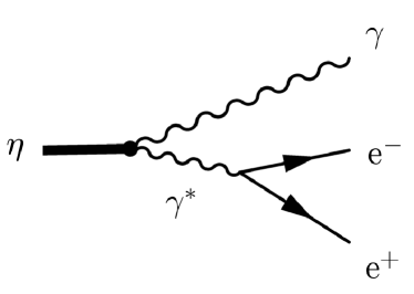
(a) In the theory of QED

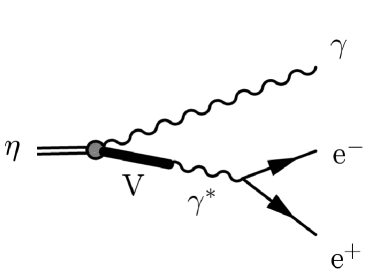
(b) In the VMD model

Fig. 1.1: Feynman diagrams showing the $\mathrm{\displaystyle}\eta\rightarrow e^{+}e^{-}\gamma$ conversion decay in two theoretical approaches. The letter V on the Feynman diagram for the VMD model denotes the neutral vector mesons (that is $\mathrm{\rho},\,\omega,\,\phi$).

1.1 The Form Factor

The study of the electromagnetic structure of particles started at the beginning of the 20th century with Rutherford’s scattering experiment and a discovery of the nucleon. Since then, the concept of the form factor plays an important role in scattering theory and appears when the scatterer is not a structure-less particle.

In the case of the transition between the $\mathrm{\displaystyle}\eta$ meson and two photons, the QED calculations give a differential cross section, in the limit where the meson is a point-like particle. The dilepton mass spectrum in the framework of the QED was firstly derived by N.M. Kroll and W. Wada in the 1950s for the $\mathrm{\pi^{0}\rightarrow e^{+}e^{-}\gamma}$ decay [19]. It can be expressed in the following form[20]:

$$\frac{d\Gamma_{l^{+}l^{-}\gamma}}{dq^{2}\cdot\Gamma_{\gamma\gamma}}=\frac{2\alpha}{3\pi q^{2}}\sqrt{1-\frac{4M_{l}^{2}}{q^{2}}}\left(1+\frac{2M_{l}^{2}}{q^{2}}\right)\left(1-\frac{q^{2}}{M_{P}^{2}}\right)^{3},$$ (1.2)

where $\mathrm{\it l}$ stands for the lepton (mion or electron), $\mathrm{\it M_{l}}$ is the lepton mass, $\mathrm{\it M_{P}}$ is the mass of the pseudoscalar meson and $\mathrm{\it q}^{2}{\it=M}^{2}_{\it l^{+}l^{-}}$ is the effective mass squared of the leptonic pair.

That is, however, only a rough approximation of reality, for all mesons are made up from quarks and gluons. To resolve this problem, all effects caused by their inner structure are introduced as an additional term in the decay amplitude, the transition form factor, $\mathrm{\it F(q}^{2})$:

$$\frac{d\Gamma_{l^{+}l^{-}\gamma}}{dq^{2}}=\left[\frac{d\Gamma}{dq^{2}}\right]_{pointlike}\cdot|F(q^{2})|^{2}.$$ (1.3)

It is a function of the square of the transferred four-momentum, $\mathrm{\it q}^{2}$, or equivalently, the square of the dilepton mass. The term transition is general for processes where a neutral meson A decays into a neutral meson B and a photon. In this case namely, the form factor reflects the effects of the electromagnetic structure arising at the $\mathrm{A}\rightarrow B$ transition vertex. The $\mathrm{\displaystyle}\eta\rightarrow e^{+}e^{-}\gamma$ is special at this point since the vertex incorporates only one meson, the one which is decaying. Therefore, the corresponding transition form factor defines the electromagnetic properties of this particular meson.

The kinematic limits for the transition form factor are determined by the masses of the particles participating in the $\mathrm{A\rightarrow B+\gamma^{*}\rightarrow B+{\it l^{+}+l^{-}}}$ process. We have:

$$(2M_{l})^{2}\leq q^{2}\leq(M_{A}-M_{B})^{2}.$$ (1.4)

Experimentally, the form factor can be determined by comparison of the measured $\mathrm{\it l^{+}l^{-}}$ differential cross section with the QED calculation for a point-like particle.

1.2 Vector Meson Dominance Model

In the Vector Meson Dominance Model, VMD, a photon is represented by a superposition of neutral vector meson states. It means that it fluctuates between an electromagnetic and a hadronic state. This approach is based on the equivalence of spin, parity and charge conjugation quantum numbers of neutral vector mesons and the photon. Hence, the coupling of photons to hadrons is determined by the intermediate neutral vector mesons as shown in the right panel of Fig. 1.1.

According to the isobar model which describes resonances by the Breit-Wigner formula [21], the form factor in the VMD model takes the following form

$$F(q^{2})=\frac{1}{\sum_{V}\frac{g_{V\eta\gamma}}{g_{V\gamma}}}\sum_{V}\frac{g_{V\eta\gamma}}{g_{V\gamma}}\frac{M_{V}^{2}}{M_{V}^{2}-q^{2}-iM_{V}\Gamma_{V}(q^{2})}\simeq\frac{1}{1-\frac{q^{2}}{M_{V}^{2}}},$$ (1.5)

where the summation index $\mathrm{V}$ runs over the $\mathrm{\rho}$, $\mathrm{\omega}$ and $\mathrm{\phi}$ vector mesons with couplings to the photon ($\mathrm{g}_{V\gamma}$) and to the $\mathrm{\eta}\gamma$ ($\mathrm{g}_{V\eta\gamma}$), and the $\mathrm{\Gamma}_{V}({\it q}^{2})$ corresponds to the total vector meson width [22, 20, 23, 24, 25]. The charge distribution inside of the meson is given by the Fourier transform of Eq. 1.5. The qualitative behavior of the electromagnetic transition form factor in the range of $\mathrm{\it q}^{2}$ is depicted in Fig. 1.2.

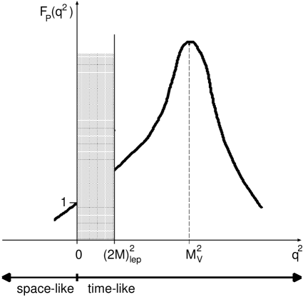
Fig. 1.2: The qualitative behavior of the electromagnetic transition form factor as a function of $\mathrm{q}^{2}$. The shaded area is the region kinematically prohibited (see Eq. 1.4). Picture is adapted from [20].

It should be noted here that study of the electromagnetic transition form factor in $\mathrm{A\rightarrow B{\it l^{+}l^{-}}}$ decays is limited to the time-like region, where the squared four-momentum of the virtual photon, $\mathrm{\it q}^{2}$ is greater than $\mathrm{(}2M_{l})^{2}$. In this case the mechanism of photon-hadron interaction is especially well pronounced since the squared four-momentum, $\mathrm{\it q}^{2}$, approaches the squared mass of the vector meson ($\mathrm{\it q}^{2}\approx{\it M_{V}^{\text{2}}}$). The virtual meson reaches its mass shell, i.e. becomes real and then decays to a lepton pair. It results in a strong resonance enhancement of the form factor of a meson. Then, at $\mathrm{\it q}^{2}>{\it M_{V}^{\text{2}}}$, the form factor begins to diminish (see Fig. 1.2).

The theoretical uncertainty of the VMD form factor in the $\mathrm{\displaystyle}\eta\rightarrow e^{+}e^{-}\gamma$ decay was estimated to be on the level of $\mathrm{5}-10$ percent [20].

1.3 Previous Experiments

The observed $\mathrm{\it q}^{2}$ distribution is fitted using a single-pole formula with parameter $\mathrm{\Lambda}_{P}$ related to the mass of the vector meson [26]:

$$F_{P}(q^{2})=\left(1-\frac{q^{2}}{\Lambda_{P}^{2}}\right)^{-1}\equiv\left(1-b_{P}^{2}q^{2}\right)^{-1}.$$ (1.6)

In the limit of small $\mathrm{\it q}^{2}$, the form factor slope parameter, $\mathrm{\it b_{P}}\equiv 1/\Lambda_{P}^{2}$ is associated with the size of the pseudoscalar meson, $\mathrm{\it b_{P}}=\langle r_{P}^{2}\rangle/6$ [20].

The currently available data on the form factor measurements, are gathered in Tab. 1.2.

		Slope parameter	Characteristic mass
Experiment	$\mathrm{N}_{events}$	$\mathrm{\Lambda}^{-2}$ [$\mathrm{G}eV^{-2}$]	$\mathrm{\Lambda}$ [$\mathrm{G}eV$]
Rutherford	50a	$\mathrm{-}0.7\pm 1.5$	$\mathrm{-}$
Laboratory[27]
SND[28]	109a	$\mathrm{1}.6\pm 2.0$	$\mathrm{-}$
CB/TAPS[29]	1345a	$\mathrm{1}.92\pm 0.35\pm 0.13$	$\mathrm{0}.720\pm 0.06\pm 0.05$
Lepton-G[30]	600b	$\mathrm{1}.9\pm 0.4$	$\mathrm{0}.724\pm 0.076$
NA-60[31]	9000b	$\mathrm{1}.95\pm 0.17\pm 0.05$	$\mathrm{0}.716\pm 0.031\pm 0.009$
VMD [26]	$\mathrm{-}$	$\mathrm{1}.78$	$\mathrm{0}.75$

• $\mathrm{\displaystyle}e^{+}e^{-}$ measured

• $\mathrm{\mu}^{+}\mu^{-}$ measured

Table 1.2: Published results of measurements of the $\mathrm{\eta}$ transition form factor with statistics of at least 50 events. In the last row, the VMD model prediction is shown.

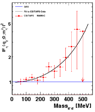
(a) Result of the CB/TAPS measurement of the $\mathrm{\displaystyle}\eta\rightarrow e^{+}e^{-}\gamma$ decay [29]

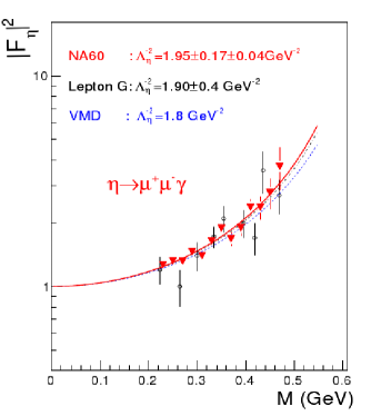
(b) Results of the Lepton-G (open circles) and the NA60 (triangles) measure-
ments of the $\mathrm{\eta}\rightarrow\mu^{+}\mu^{-}\gamma$ decay. The solid and dashed-dotted lines are fits to the NA60 data while the dotted line is the VMD model prediction. Picture is taken from [31]

Fig. 1.3: The squared transition form factor of the $\mathrm{\displaystyle}\eta$ meson as a function of the lepton pair mass, obtained in the CB/TAPS, Lepton-G and NA60 experiments for $\mathrm{\displaystyle}\eta\rightarrow e^{+}e^{-}\gamma$ and $\mathrm{\eta}\rightarrow\mu^{+}\mu^{-}\gamma$ decays.

Nearly 9000 of $\mathrm{\eta}\rightarrow\mu^{+}\mu^{-}(\gamma)$ events were reconstructed in the NA60 experiment using data taken in 2003 for In-In collisions [31]. It has to be noted here that in this experiment, the photon was not measured and therefore the meson was not fully reconstructed but obtained from unfolding the $\mathrm{\mu}^{+}\mu^{-}$ mass spectrum. The same decay channel was studied with the Lepton-G experiment [30]. However, since those measurements concern muons, the lower kinematic limit of the squared four-momentum transfer is much higher than in case of electrons and there is no information below $\mathrm{{\it q}^{2}{\it\equiv M=(}2{\it M_{\mu})}^{2}=(0.23~{}GeV/c^{2})^{2}}$ (see Eq.1.4). This can be seen in Fig. 1.3b where both results are shown.

As regards the $\mathrm{\displaystyle}\eta\rightarrow e^{+}e^{-}\gamma$ decay, in two experiments the number of reconstructed $\mathrm{\displaystyle}\eta\rightarrow e^{+}e^{-}\gamma$ mesons exceeded the level of hundred events. One measurement was carried out with the SND detector on the VEPP-2M collider in Novosibirsk, in the years 1996 and 1998 [28]. Only 109 of $\mathrm{\displaystyle}\eta\rightarrow e^{+}e^{-}\gamma$ events were reconstructed, resulting in the determination of the form factor slope $\mathrm{\it b_{P}}=(1.6\pm 2.0)~{}GeV^{-2}$. The most recent result, obtained from the analysis carried out in parallel to this work, concerns the measurement performed at the MAMI-C accelerator using the combined Crystal Ball (CB) and TAPS detectors. Although there is no magnetic field available for particle tracking and hence, the sign of the charged particle cannot be determined, the $\mathrm{1}345$ of $\mathrm{\displaystyle}\eta\rightarrow e^{+}e^{-}\gamma$ mesons produced in the $\mathrm{\gamma}p\rightarrow p\eta\rightarrow pe^{+}e^{-}\gamma$ reaction were reconstructed and a value of $\mathrm{\it b_{P}}=(1.92\pm 0.35\pm 0.13)~{}GeV^{-2}$ has been determined [29]. The form factor, extracted from CB/TAPS data, together with the single-pole approximation, is shown in Fig. 1.3a.

Chapter 2 Experimental Setup

2.1 The COSY Storage Ring

The data used for the analysis in this work, were taken at the Research Center Jülich, in Germany. The measurement was carried out using the WASA[11] detector installed at the COoler SYnchrotron COSY [32, 12]. The COSY ring is a 184 m circumference accelerator which provides beams of protons and deuterons (also polarized), in the momentum range from $\mathrm{0}.3$ GeV/c to $\mathrm{3}.7$ GeV/c [33].

A floor plan of the COSY facility is shown in Fig. 2.1. The JULIC cyclotron delivers either $\mathrm{H}^{-}$ or $\mathrm{D}^{-}$ ions pre-accelerated up to the momentum of $\mathrm{0}.3$ GeV/c. Up to $\mathrm{1}0^{11}$ particles injected by the cyclotron can be then stored in the COSY ring which, in the case of internal pellet targets, allows for luminosities of $\mathrm{1}0^{32}~{}cm^{-2}~{}s^{-1}$.

For reducing the beam momentum spread and to compensate the mean energy loss, three methods of beam cooling are available. Electron cooling is applied in case of protons with momenta up to $\mathrm{0}.6~{}GeV$. To obtain well focused beams of particles with momenta above $\mathrm{1}.5$ GeV/c, stochastic cooling is used [34]. Stochastic cooling allows to achieve a beam momentum resolution, $\mathrm{\Delta}p/p$, below $\mathrm{1}0^{-4}$. For experiments with thick targets of more than $\mathrm{1}0^{15}~{}atoms/cm^{2}$, also the barrier bucket cavity method is applied [35].

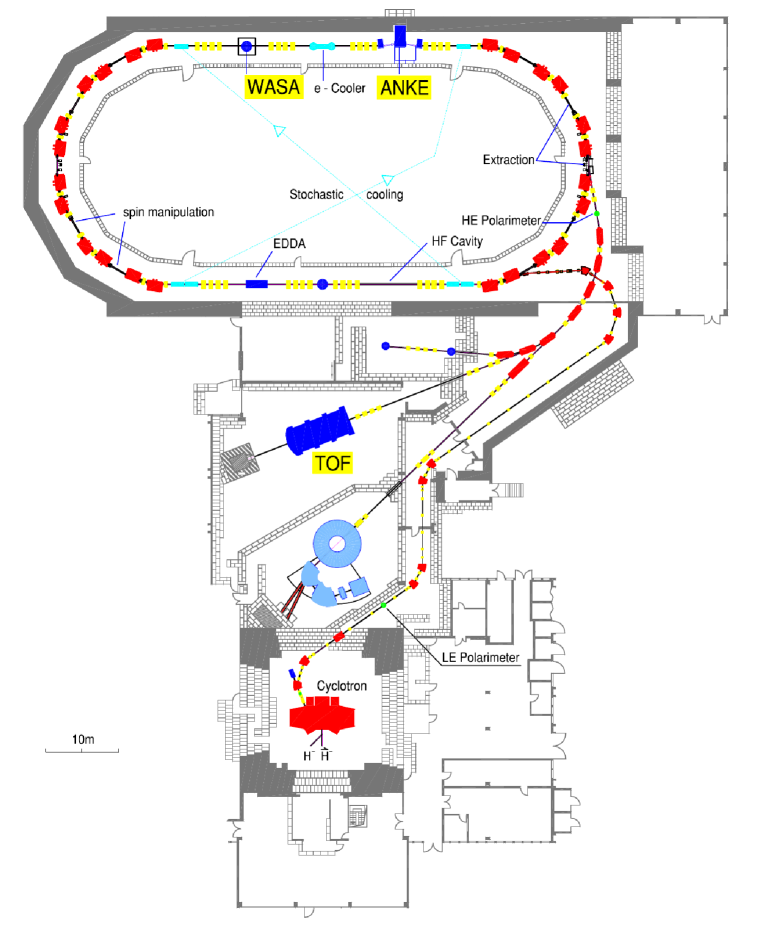
Fig. 2.1: Schematic view of the COSY facility. The WASA detector [11] is situated in the COSY ring, next to the ANKE experiment [36] and opposite to the EDDA experiment [37]. Further down in the picture the location of the TOF detector [38] is marked. Below it, there is the JULIC Cyclotron.

2.2 The WASA detector

The WASA detector is one of the internal detectors of COSY. Up to 2005, it was operating at the CELSIUS storage ring in Sweden [39]. After the shutdown of the accelerator, the detector was moved to Jülich and mounted in COSY where it has been taking data since 2007 [40, 41, 42, 43, 44].

The physics program aims at pursuing the knowledge of hadron structure and symmetry breaking in QCD, in the sector of the up, down and strange quarks [11]. The main interest is to study rare $\mathrm{\displaystyle}\eta$, $\mathrm{\eta}^{\prime}$ and $\mathrm{\omega}$ decays, which provides an understanding of structure of matter and hadron dynamics.

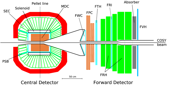
Fig. 2.2: Overview of the WASA detector. The names abbreviations of the detector elements are explained in the text. See also the List of Acronyms.

For that purpose, WASA is equipped with a set of plastic scintillators, straw tubes and an electromagnetic calorimeter which covers almost full $\mathrm{4}\pi$ solid angle in the laboratory frame. The arrangement of the detector components is optimized to tag a reaction via the recoil particle going to the forward part of the detector, and to register meson decay products in the central part of the detector. Therefore, the two parts of WASA are called forward (FD) and central (CD) detector, respectively.

The overview of the detector’s layout is shown in Fig. 2.2.

2.2.1 Central Detector

The central detector surrounds the interaction point. It is designed for the detection of particles being the products of the decays of produced mesons. The straw tube detector (Mini Drift Chamber - MDC) together with the solenoid, serves as a source of information about charged particles’ momenta. The plastic scintillators (Plastic Scintillator Barrel - PSB) and a calorimeter (SEC) deliver information about energy deposited by particles. The calorimeter is used for identification of photons as well.

2.2.1.1 Mini Drift Chamber

The MDC is placed around the beam pipe, inside the solenoid, and covers scattering angles from $\mathrm{2}4$ to $\mathrm{2}59$ degrees. It consists of 1738 straws arranged in 17 layers (see Fig. 2.3a). In nine of the layers the straws are aligned parallel to the beam axis while in the remaining layers they are placed with a small skew angle of $\mathrm{2}$-$\mathrm{3}$ degrees (see also [45]).

Straws are made of $\mathrm{2}5~{}\mu m$ Mylar foil aluminized on the inner side. Sense wires are made of gold plated tungsten and have a diameter of $\mathrm{2}0~{}\mu m$. Thanks to the potential difference between the wire (kept at high voltage) and the grounded walls, electrons start to move towards the wire while ions in the direction of the wall. The resulting electrical current indicates that a particle was passing the tube.

The gas mixture used to fill the tubes consist of $\mathrm{8}0\%$ argon and $\mathrm{2}0\%$ ethane. It was chosen so, that any particle passing through it causes its ionization. It provides linear correlation of the drift time to the drift distance with a relatively low operating voltage.

The MDC operates in a magnetic field of the superconducting solenoid (SEC), under the action of which, the particles trajectories undergo bending. The MDC allows to extract particle trajectory parameters, the angles, momenta and the vertex position.

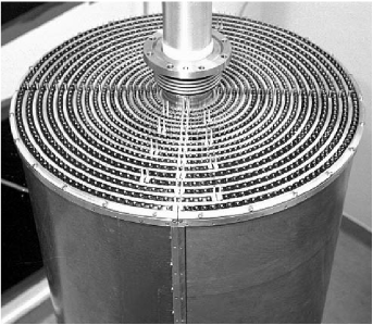
(a) The MDC inside the Al-Be cylinder

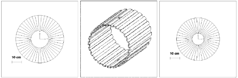
(b) Schematics of the forward (left), central (middle) and backward (right) parts of the PSB

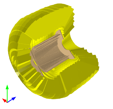
(c) Schematic view of the SEC

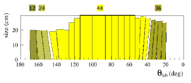
(d) Angular coverage of the SEC. The number of crystals in each ring is indicated by numbers above the picture

Fig. 2.3: Components of the Central Detector of the WASA setup.

2.2.1.2 Plastic Scintillator Barrel

The three parts of the PSB surround the drift chamber (see Fig. 2.3b). Each of the two end-cups is composed of 48 trapezoidal elements with a hole in the center designated for the beam pipe. The central part is comprised of 52 bars forming two layers with a small overlap between elements.

Together with the MDC it is used for the identification of charged particles by the $\mathrm{\Delta}E-p$ (energy-momentum) method.

2.2.1.3 Superconducting Solenoid

The Superconducting Solenoid encloses the volume of the MDC and the PSB. The magnetic field produced by it has a maximum of $\mathrm{1}.3$ T. It is cooled with liquid helium. It serves for the calculation of momenta of charged particles registered in the MDC. A detailed description of the solenoid can be found in [46].

2.2.1.4 Scintillating Electromagnetic Calorimeter

The Scintillating Electromagnetic Calorimeter (SEC) is the outermost component of the central detector. It consists of 1012 sodium-doped CsI scintillating crystals covering a polar angle from $\mathrm{2}0$ to $\mathrm{1}69$ degrees (see Fig. 2.3d). The crystals are arranged in 24 layers perpendicular to the beam pipe in the center part and with the inclination growing with the distance from the center. The length of the crystals varies based on their location. The shortest ones, of $\mathrm{2}0$ cm length, are placed in the backward part, the ones of $\mathrm{2}5$ cm length in the forward part and the longest ones ($\mathrm{3}0$ cm) compose the central part (see Fig. 2.3c).

The calorimeter energy resolution for photons is given by $\mathrm{\frac{missing}{missing}}{\sigma_{E}}{E}=\frac{5\%}{\sqrt{E/GeV}}$. The angular resolution is limited by the crystal size to $\mathrm{5}$ degrees in the scattering angle [39].

A detailed description of the calorimeter can be found e.g. in Ref. [47].

2.2.2 Forward Detector

The forward detector is used for the detection of charged recoil particles like protons, deuterons and helium ions. It consists of a set of plastic scintillators and a straw tube tracker, so that it allows for particle identification and four-momentum reconstruction of recoils, scattered in the range of the polar angle from $\mathrm{3}$ to $\mathrm{1}8$ degrees.

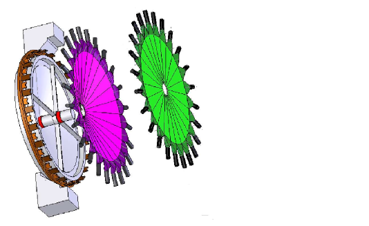
(a) The Forward Window Counter, exploded view

(b) Schematic view on the arrangement of the Forward Proportional Chamber modules

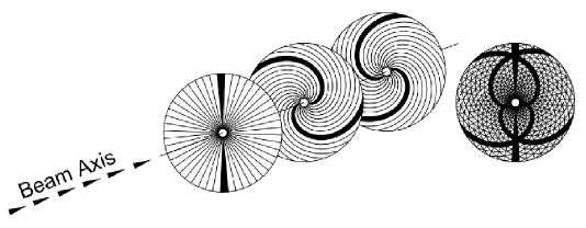
(c) Left: three layers of the Forward Trigger Hodoscope hit by two particles. Right: projection on the xy-plane, intersections of struck elements define pixels

Fig. 2.4: Components of the Forward Detector of WASA.

2.2.2.1 Forward Window Counter

The Forward Window Counter, FWC, is part of the forward detector placed closest to the interaction region. These are $\mathrm{4}8$ plastic scintillators arranged in two layers shifted by half an element with respect to each other. In addition, the first layer is placed with a small inclination in order to mimic the shape of the exit window of the central detector (see Fig. 2.4a and [48]).

The FWC is one of the detectors involved in the identification of helium ions via the $\mathrm{\Delta}E-E$ method. It is also a very important component of the trigger in experiments with $\mathrm{\displaystyle}\,{}^{3}He$ as a recoil particle, in which case, the selection of events is based on the fact that the $\mathrm{\displaystyle}\,{}^{3}He$ is characterized by a bigger energy loss in the FWC in comparison with other, lighter particles.

2.2.2.2 Forward Proportional Chamber

Directly after the FWC, the Forward Proportional Chamber is located. It is made up of $\mathrm{1}952$ straws grouped into sixteen layers, every of $\mathrm{9}2\times 92~{}cm^{2}$ sensitive area. Each subsequent four layers correspond to one module. Straws in layers of each module are shifted by $\mathrm{\pm}$ tube radius in respect to the straws of neighboring layers. The modules are rotated with respect to the x-axis by $\mathrm{3}15$, $\mathrm{4}5$, $\mathrm{0}$ and $\mathrm{9}0$ degrees, respectively, as shown in Fig. 2.4b.

The last two modules alone give already the information about the x and y coordinates of passing particle. Adding the first two modules allow in addition, to improve the spatial resolution, estimate the track coordinates and to reduce noise. A detailed description of the FPC can be found in Ref. [49].

2.2.2.3 Forward Trigger Hodoscope

The Forward Trigger Hodoscope consists of three layers of plastic scintillators. The first layer, closest to the interaction point, is built up from $\mathrm{4}8$ elements. Two subsequent ones consist of elements curved into archimedian spirals oriented clockwise and counter-clockwise (see Fig. 2.4c).

A particle passing through the FTH, leaves a trace in the form of a hit in elements of consecutive layers. Three layers projected onto the xy-plane give an intersection point of struck elements, called pixel.

The first layer of the FTH is used to activate the trigger signal and further to determine the azimuthal angle of the particle trajectory. The FTH is also used in identification of the recoil particle(s) in the forward detector via the $\mathrm{\Delta}E-E$ method. More detailed information about the design and performance of this detector can be found in Ref. [50].

2.2.2.4 Forward Range Hodoscope

The Forward Range Hodoscope consists of five layers made of $\mathrm{2}4$ plastic scintillators each (see Fig. 2.5). The first three layers are of $\mathrm{1}10$ mm thickness while the last two are $\mathrm{4}0$ mm thicker. This detector is used for the identification of a recoil particle(s) with the $\mathrm{\Delta}E-E$ method and together with the FWC and the FTH, it is used in the trigger to check the track alignment in the azimuthal angle.

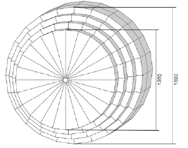
Fig. 2.5: The Forward Range Hodoscope.

2.2.2.5 Forward Veto Hodoscope

The Forward Veto Hodoscope is made of twelve, horizontally aligned bars of plastic scintillators each of which being $\mathrm{2}$ cm thick and $\mathrm{1}3.7$ cm wide. It is used to reject particles, punching through the Range Hodoscope and therefore, it increases the trigger selectivity.

2.2.3 The Pellet Target

The special - Pellet Target - system was developed for the WASA experiment to satisfy the conditions required by a $\mathrm{4}\pi$ detector [51]. It was designed to keep as less of the material inside of the detector as possible and therefore most of it, is located outside the detector. Only the $\mathrm{2}$ meters long, $\mathrm{7}$ mm narrow pellet beam tube, crosses the scattering chamber, delivering pellets to the impact point (see Fig. 2.6). A target in form of pellets was chosen to achieve luminosities of the order of $\mathrm{1}0^{32}~{}cm^{-2}~{}s^{-1}$, needed to study rare decays of light mesons, the beam target in the form of a gas or a cluster jet is not enough good collimated.

Fig. 2.6: Schematic view of the WASA Pellet Target system.

In order to obtain a stream of pellets of the same size and with the same distance separating them, the high-purity liquid jet is broken up by vibrations of a thin glass nozzle located in the pellet generator.

The achieved divergence of the target beam is on the order of $\mathrm{0}.04^{\circ}$, the single pellet size amounts to about $\mathrm{3}5~{}\mu$m. Together with the effective areal target thickness greater than $\mathrm{1}0^{15}~{}atoms\cdot cm^{-2}$, the luminosities of $\mathrm{1}0^{32}~{}cm^{-2}~{}s^{-1}$ are becoming feasible.

2.2.4 Data Acquisition System

The Data Acquisition system (DAQ) collects and process signals from the detector elements, in order to make them available for further analysis. The structure of the Data Acquisition system is shown in Fig. 2.7.

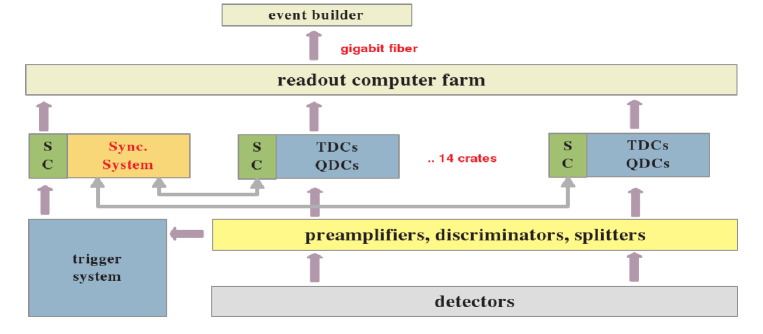
Fig. 2.7: Structure of the Data Acquisition system.

Signals from 3800 straws and 1570 photomultiplier tubes connected with detector elements, are distributed and adapted by electronic modules of the lowest layer of the Data Acquisition system ( pre-amplifiers, splitters, discriminators). Next, the conversion of analogue signals is done in fourteen crates of the digitization layer. There, the digitized signal is marked with a timestamp as well, and queued in FIFOs .

The timestamp is broadcasted by a special module (master module) of the main synchronization system. To this module also, the first level trigger is connected. Invoked by the trigger, the master module computes the event number and sends it, together with the timestamp, to all fourteen crates, where digitized information, also marked with the timestamp, wait in FIFOs. While the crates are processing received information, the master module blocks the trigger.

Data with a matching timestamp, marked with an event number, are passed to the readout computer farm and to the event builder. More detailed information on the performance and the operation of the Data Acquisition system can be found in [52, 53].

Chapter 3 Analysis Tools

3.1 Root

The software package Root [54] is the most used tool in this work. It is a successor of the, FORTRAN implemented, Physics Analysis Workstation (PAW)[55], developed in the European Organization for Nuclear Research (CERN) [56]. All the histogramming, fitting, calculations were done using its object oriented, C++ operated structure.

3.2 Event Generator

For the purpose of studies made in this work, the Pluto++ [57] event generator was used. It is a collection of C++ classes based on the ROOT [58] environment.

The event generator generates the pseudoscalar meson Dalitz decays with a virtual photon (described by the $\mathrm{\phi}_{\gamma}^{*}$ and $\mathrm{\theta}_{\gamma}^{*}$ angles) being isotropically distributed in space, carrying a momentum determined by its invariant mass and the mass of the meson (see Fig. 3.1).

Fig. 3.1: The picture shows four angles which need to be taken into account while considering $\mathrm{\gamma}^{*}\rightarrow e^{+}e^{-}$ conversion. More details are given in the text. Picture is taken from [59].

The azimuthal angle, $\mathrm{\phi}_{e}^{ee}$, of the dilepton decay plane around the photon direction is isotropic, while the helicity angle - $\mathrm{\theta}^{ee}_{e}$ is distributed according to $\mathrm{1}+cos^{2}\theta^{ee}_{e}$[60].

The invariant mass spectrum of lepton-antilepton pairs is given according to [20] by equation 1.2, see Sec. 1.1. The Pluto++ event generator enables also modifications in the spectrum due to the presence of a given form factor.

3.3 Detector Simulation

For the reproduction of the detector response, the WASA Monte Carlo software is used. It is based on the GEANT package [61].

The description of the detector components (theirs dimensions, positions, type of the material, magnetic field) has been implemented in the GEANT framework while the reaction kinematics (the initial four-momenta of particles) is delivered by the event generator.

The WASA Monte Carlo takes into account such effects like energy loss, multiple scattering and conversion in the detector material. In addition, it is possible to improve the matching between data and simulations via smearing of the simulated observables according to the known resolution of detectors.

Within preparations to work with experimental data, the algorithms created for the purpose of the form factor extraction were tested on the Monte Carlo sample of $\mathrm{1}0^{6}$ events of the $\mathrm{\displaystyle}pd\rightarrow{}^{3}He\,\eta\to{}^{3}He\,\gamma\,e^{-}e^{+}$ reaction. Fig. 3.2 shows the distribution of the invariant mass of the $\mathrm{\displaystyle}e^{+}e^{-}$ pairs generated with Pluto++ and then reconstructed by the WASA analysis software before and after acceptance corrections. The correctness of developed procedure manifests itself on the right panel of this figure, where all points are situated on the QED line, as expected. Having constructed a properly working method of the determination of the variable of interest, one can start a thorough analysis of experimental data.

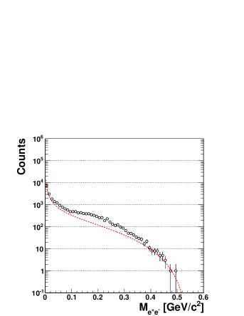
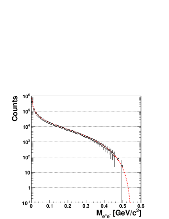
Fig. 3.2: Simulated and then reconstructed lepton-antilepton mass spectrum (left), acceptance corrected (right). $\mathrm{1}0^{6}$ events (circles) were generated using the Pluto++ event generator with a form factor equal to one and then processed by the WASA Monte Carlo software which reproduces the experimental environment. The dotted, red line shows the calculation according to the QED.

Chapter 4 First Stage Event Reconstruction

4.1 Trigger Conditions

The $\mathrm{\displaystyle}\eta$ mesons were produced in the $\mathrm{\displaystyle}pd\rightarrow{}^{3}He\,\eta$ reaction with a beam momentum of $\mathrm{1}.7$ GeV/c which corresponds to an excess energy of $\mathrm{6}0$ MeV. The cross section for the $\mathrm{\displaystyle}\eta$ meson production at this energy amounts to $\mathrm{0}.412\pm 0.016\,\mu b$ [62]. That leads to an event rate which makes it possible to use an unbiased trigger. It means, that the trigger logic was fully based on signals coming from the components of the forward part of the detector and therefore, no requirements on the meson decay products were used.

The requirement was at least one charged particle with a minimum energy loss of $\mathrm{5}$ MeV in the Forward Window Counter. This particle must have had signature also in the first layers of the Forward Trigger Hodoscope and the Forward Range Hodoscope. Hits in all those three detectors had to be aligned with the same azimuthal angle.

4.2 Track Reconstruction

Signals invoked in the detectors by particles passing through them are merged into tracks using reconstruction algorithms. Merging is done within given boundaries regarding time, energy deposits and angular information. Their default values have been chosen to provide the best quality of reconstruction [11]. Nevertheless, it must be checked and, if necessary, also tuned for each experimental run, especially when coming to study of some specific reaction channel characterized by small branching ratio.

4.3 Track of the Recoil Particle

In the case of the $\mathrm{\displaystyle}pd\rightarrow{}^{3}He\,\eta$ reaction, the recoil particle is the helium ion going in the forward direction. The reconstruction of tracks in the Forward Detector begins with combining time coincident hits in adjacent detector elements into larger groups called clusters. This is necessary since particles passing a detector close to the border of a given element, can cause a signal in the adjacent one. Having all hits assigned to the cluster, the geometrical overlap between clusters formed in different layers of the detector can be checked. The procedure starts from taking the Forward Trigger Hodoscope pixel (see Fig.2.4c) and searches the detector in order to find overlapping clusters. The Forward Trigger Hodoscope also serves as a source of the initial information about the angular coordinates. The reconstruction procedure assumes a vertex located in the center of a nominal beam and target interaction region. Next, the angular information of the track can be improved based on signals from the Forward Proportional Chamber. The time assigned to the track is taken as the average time of hits contributing to the Forward Trigger Hodoscope pixel.

4.4 Tracks of Meson Decay Products

Particles coming from the decay of the $\mathrm{\displaystyle}\eta$ meson are registered in the Central Detector. The track reconstruction starts in the calorimeter. All hits are combined into clusters according to their position, energy and relative time. Typically, the allowed limits for the hits to be enclosed in a cluster are: i) a time difference with the central module of $\mathrm{5}0~{}ns$ and, ii) a minimum energy of $\mathrm{2}~{}MeV$.

The starting crystal, the center of the cluster, is the one with the highest energy deposit (minimum of $\mathrm{5}~{}MeV$) and its time defines the time of the cluster. Hits in crystals adjoining it, are added to it, if they were not included already in another cluster.

The formed cluster’s energy, is the sum of energies from the contributing crystals. It has to be more than $\mathrm{5}~{}MeV$. The cluster position is given by the energy weighted mean of the positions of crystals constituting it. If there are no matching clusters found in the Mini Drift Chamber and Plastic Scintillator Barrel, the cluster is assigned as coming from a neutral particle. More detailed description of the cluster reconstruction in the Scintillating Electromagnetic Calorimeter can be found in [63].

A cluster in the Plastic Scintillator Barrel constitutes a single hit or, in case of overlapping elements, two hits if the deposited energy amounts to at least $\mathrm{1}~{}MeV$ and their time difference is less than $\mathrm{1}0~{}ns$.

Particles in the magnetic field follow a helical trajectory. Therefore, hits registered in the Mini Drift Chamber are described with helices. Hits belonging to one helix create a cluster. The procedure of extracting all the helix parameters, consists of two main steps. First, hits are projected onto the xy plane (perpendicular to the beam axis) and fitted with circles. Next, a straight line is fitted to the hits in the Rz plane. Description of the algorithm can be found in Ref. [64].

Having grouped the information in all three subdetectors of the Central Detector, the track assignment can be done. That is, clusters formatted in the Mini Drift Chamber, the Plastic Scintillator Barrel and the Scintillating Electromagnetic Calorimeter are checked with regard to their belonging to one track. The geometric overlap of clusters is used as a criterion.

In case of the Mini Drift Chamber and the Plastic Scintillator Barrel the criterion is difference of the azimuthal angles $\mathrm{\Delta}\phi$ between the exit coordinate of the helix and position of the cluster in the Plastic Scintillator Barrel. The experimental distribution of $\mathrm{\Delta}\phi$ is shown in Fig. 4.1a. A window of $\mathrm{|}\Delta\phi|<20^{\circ}$ was conservatively applied.

Matching between the Mini Drift Chamber and the Scintillating Electromagnetic Calorimeter is done by building a straight line, tangential to the helix in its exit point, and calculating its position at the calorimeter surface. The angular difference between this position and the position given by the calorimeter cluster is the matching criterion. The relevant, experimental distribution is shown in Fig. 4.1b. Small peaks seen over the whole range of the x-axis are caused by the detector granularity. A maximum opening angle of $\mathrm{2}5^{\circ}$ is selected.

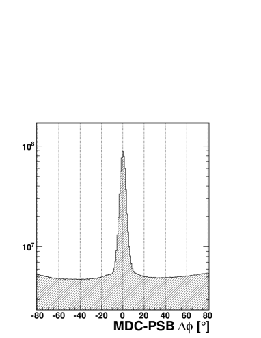
(a) The difference in the azimuthal angle between the Mini Drift Chamber and the Plastic Scintillator Barrel. The cut was chosen to $\mathrm{|}\Delta\phi|<20^{\circ}$

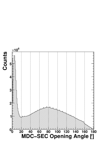
(b) The opening angle between the Mini Drift Chamber and the Scintillating Electromagnetic Calorimeter was chosen to be less than $\mathrm{2}5^{\circ}$

Fig. 4.1: Experimental distributions used to choose the matching conditions in the Central Detector. The track assignment in the Central Detector consist in checking for geometric overlaps of chamber’s cluster with clusters in the Plastic Scintillator Barrel and the Scintillating Electromagnetic Calorimeter.

Chapter 5 Extraction of the Signal Channel

In case of the $\mathrm{\displaystyle}pd\rightarrow{}^{3}He\,\eta\to{}^{3}He\,\gamma\gamma^{*}\to{}^{3}He\,\gamma\,e^{-}e^{+}$ reaction, particle identification consists in recognizing three tracks and an additional cluster in the SEC. The $\mathrm{\displaystyle}\,{}^{3}He$ ion is identified using the forward part of the WASA detector while $\mathrm{e}^{+}$, $\mathrm{e}^{-}$ and $\mathrm{\gamma}$ particles coming from the $\mathrm{\displaystyle}\eta$ decay, are detected and reconstructed in the central part of the detector.

5.1 Kinematics - Phase Space

In the used Monte Carlo events generator, Pluto++, it is assumed that the phase space in $\mathrm{\displaystyle}pd\rightarrow{}^{3}He\,\eta$ production is homogeneously and isotropically populated. In Fig. 5.1a one can see the flat distribution of the cosine of the $\mathrm{\displaystyle}\eta$ scattering angle in the center of mass system as it comes from the generator whereas, in Fig.  5.1b the helium scattering angle in the center of mass system as a function of the $\mathrm{\displaystyle}\,{}^{3}He$ scattering angle in the laboratory system is shown. The dashed line corresponds to the geometrical acceptance of the Forward Detector. Helium particles which were scattered in the laboratory system under a $\mathrm{3}^{\circ}$ angle, are not seen in the detector. One may notice also, that $\mathrm{\displaystyle}\,{}^{3}He$ particles produced in the $\mathrm{\displaystyle}pd\rightarrow{}^{3}He\,\eta$ reaction at a beam momentum of $\mathrm{1}.7$ GeV/c are emitted up to the $\mathrm{\sim}10^{\circ}$ of scattering angle, so well below $\mathrm{1}8^{\circ}$ which is the upper geometrical limit of the Forward Detector.

The overall geometrical acceptance of the WASA detector for registering all four particles in a given event, coming from the $\mathrm{\displaystyle}pd\rightarrow{}^{3}He\,\eta\to{}^{3}He\,\gamma\,e^{-}e^{+}$ reaction, amounts to almost $\mathrm{8}0\%$.

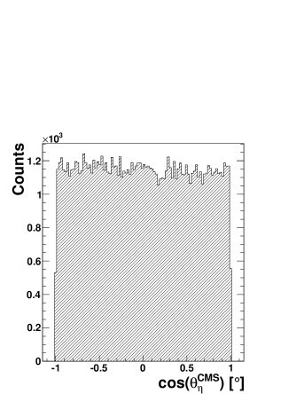
(a) Generated spectrum showing the cosine of the $\mathrm{\displaystyle}\eta$ scattering angle in the center of mass system (CMS)

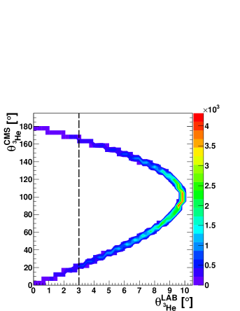
(b) Generated spectrum showing the $\mathrm{\displaystyle}\,{}^{3}He$ scattering angle, in the center of mass system (CMS) as a function of the $\mathrm{\displaystyle}\,{}^{3}He$ scattering angle in the laboratory system (LAB)

Fig. 5.1: The output of the Pluto event generator for the $\mathrm{\displaystyle}pd\rightarrow{}^{3}He\,\eta$ reaction. About 5% of generated events is outside of the Forward Detector geometrical acceptance shown in (5.1b) as a dashed line.

5.2 Identification of Helium

$\mathrm{\displaystyle}\,{}^{3}He$ is detected and reconstructed in the Forward Detector. Already on the preselection level, helium ions were initially identified. However, this identification was done using a rough calibration [65]. Therefore, additional checks are made.

In the first step, appropriate minimal energy deposits in each of the detectors are set. This is done based on experimental spectra of energies deposited in each layer of the detector as shown in Fig. 5.2.

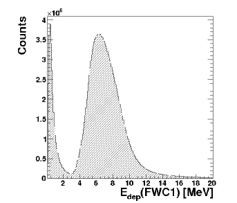
(a) Energy deposited in FWC1

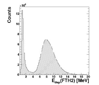
(b) Energy deposited in FTH2

Fig. 5.2: Energy depositions in experiment for the first layer of the Forward Window Counter (5.2a) and the second layer of the Forward Trigger Hodoscope (5.2b). Cut on minimal deposited energy was chosen to $\mathrm{3}~{}MeV$ in the FWC1 and $\mathrm{4}~{}MeV$ in the FTH2.

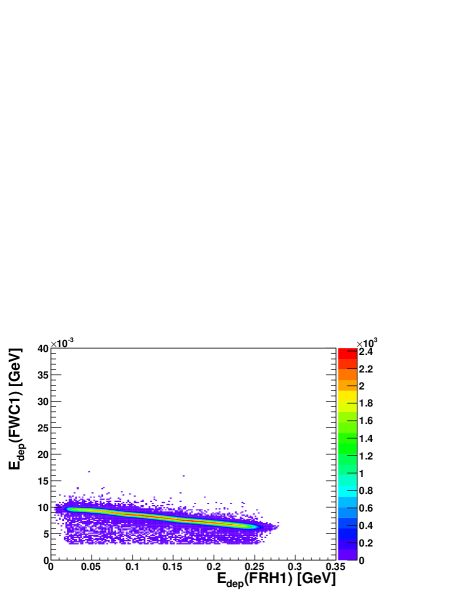
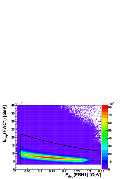
Fig. 5.3: $\mathrm{\Delta}{}E-E$ plots of energy deposited in the first layer of the Forward Window Counter and the first layer of the Forward Range Hodoscope used for the final helium selection. In the upper panel simulated data are presented while the bottom plot shows experimental data. Particles, having energy depositions within boundaries shown in the picture with black lines, are considered further as helium ions.

Candidate for a helium track must have also the scattering angle within geometrical boundaries of the Forward Detector.

Finally, to select tracks of $\mathrm{\displaystyle}\,{}^{3}He$ particles, the $\mathrm{\Delta}{}E-E$ method is used. Multilayered architecture of the Forward Detector allows to perform identification, based on energy losses in different layers of the detector. Correlation of energy deposited in the first layer of the Forward Window Counter and the first layer of the the Forward Range Hodoscope is shown in Fig. 5.3.

In order to convert deposited energy into kinetic energy a set of parameters were derived from the Monte Carlo simulations. This correction parameters are needed since due to the occurrence of additional energy losses in the detector material, the sum of deposited energies can be smaller than the true kinetic energy.

For this purpose, the Monte Carlo simulation of single particle tracks was used and the relative difference of the reconstructed deposited energy and the true kinetic energy was parametrized as a function of the deposited energy.

In case of the $\mathrm{\displaystyle}pd\rightarrow{}^{3}He\,\eta$ reaction with the beam momentum of $\mathrm{1}.7~{}GeV/c$, the kinetic energy in units of GeV may be described by equation 5.1:

$$E_{kin}(E_{dep},\theta)=(c_{0}+c_{1}E_{dep}+c_{2}E_{dep}^{2}-c_{3}E_{dep}^{3})(a_{0}-a_{1}cos\theta),$$ (5.1)

where $\mathrm{c}_{0}=0.199876,\,c_{1}=0.640187,\,c_{2}=1.60489,\,c_{3}=2.28946,\,a_{0}=1.42133$, $\mathrm{a}_{1}=0.364951$ and $\mathrm{E}_{dep}$ is the energy deposited in the Forward Range Hodoscope expressed in GeV and $\mathrm{\theta}$ is the scattering angle [66].

5.3 Identification of Photon

Selection of a neutral particle in the Central Detector, starts with checking its time correlation with the $\mathrm{\displaystyle}\,{}^{3}He$, selected in the Forward Detector. Time cut of [-24,20] ns was chosen (see Fig. 5.4).

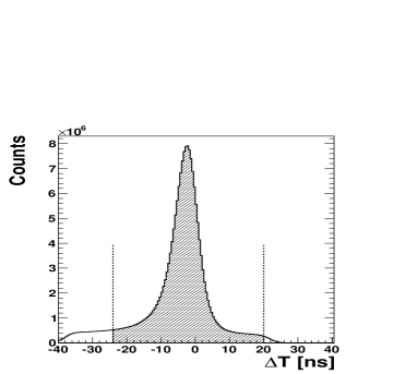
Fig. 5.4: Experimental distribution of the time difference, $\mathrm{\Delta}T$, between $\mathrm{\displaystyle}\,{}^{3}He$ in the Forward Detector and the neutral particle in the Central Detector. Dashed line shows the time cut used in the analysis.

Cluster in the SEC without an associated track in the MDC can originate not only from the $\mathrm{\gamma}$ coming from the impact point but also from the interaction of charged particle in the detector material. So-called split-off, is characterized by small energy and a small angle to the nearest charged particle. Energy of the photon candidate presented as a function of the angle it creates with the nearest charged particle, $\mathrm{\Omega}$, is shown in Fig. 5.5. The Monte Carlo distribution in the right panel consists of events from the simulated $\mathrm{\displaystyle}pd\rightarrow{}^{3}He\,\eta\to{}^{3}He\,\gamma\gamma^{*}\to{}^{3}He\,\gamma\,e^{-}e^{+}$ reaction. The signal is visible in the upper right part of the picture. At the $\mathrm{\Omega}\sim 20^{\circ}$ an enhancement caused by split-offs appears. The same distribution from the experiment, shown in the left panel, is strongly contaminated. In order to cut out events with false photon candidates, the restriction on the $\mathrm{\Omega>60^{\circ}}$ and $\mathrm{E_{\gamma}>0.1-0.00055*\Omega}$ was applied as indicated by lines in Fig. 5.5b.

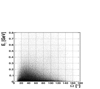
(a) The experiment

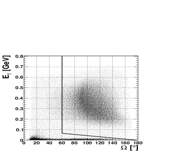
(b) Simulation of the $\mathrm{\displaystyle}pd\rightarrow{}^{3}He\,\eta\to{}^{3}He\,\gamma\,e^{-}e^{+}$ reaction

Fig. 5.5: Spectra of cluster’s energy vs. the angle it creates with the nearest track.

The fact that products of the $\mathrm{\displaystyle}\eta\rightarrow\gamma\gamma^{*}$ decay fly back-to-back in the meson rest frame, is applied in further selection on the remaining set of neutral particles reconstructed in Central Detector. That is, each of photon candidate is checked for the azimuthal angle it creates with the virtual photon in the $\mathrm{\displaystyle}\eta$ rest frame. The four-momentum of the virtual photon is reconstructed based on four-momentum vectors of $\mathrm{e}^{+}$ and $\mathrm{e}^{-}$. In the $\mathrm{\displaystyle}\eta$ meson rest frame, real and virtual photon create the opening angle $\mathrm{\Delta}\phi_{\gamma\gamma*}$ of $\mathrm{1}80^{\circ}$.

In order to check the $\mathrm{\Delta}\phi_{\gamma\gamma*}$ reconstruction resolution, the histogram in Fig. 5.6 was filled with values calculated as $\mathrm{\Delta}\phi_{\gamma\gamma*}^{true}-\Delta\phi_{\gamma\gamma*}^{reconstructed}$. The FWHM of the distribution is $\mathrm{\sim 9^{\circ}}$.

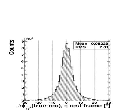
Fig. 5.6: Simulated distribution of the difference between true and reconstructed values of the azimuthal angle between real and virtual photon in the $\mathrm{\displaystyle}\eta$ rest frame, $\mathrm{\Delta}\phi_{\gamma\gamma*}=\Delta\phi_{\gamma\gamma*}^{true}-\Delta\phi_{\gamma\gamma*}^{reconstructed}$.

Fig. 5.7 shows experimental distributions of $\mathrm{\Delta}\phi_{\gamma\gamma*}$ with and without usage of the charged particle identification ( see Section 5.4, Fig. 5.11b ). If in a given event more than one photon candidate was identified, then it was also included in the picture. The cut was chosen conservatively in the range of $\mathrm{[}70,290]$ degrees of $\mathrm{\Delta}\phi_{\gamma\gamma*}$ difference as shown by vertical lines in Fig. 5.7. Application of the $\mathrm{\displaystyle}e^{+}e^{-}$ identification causes, that the signal channel is more pronounced and, therefore, the $\mathrm{\Delta}\phi_{\gamma\gamma*}$ distribution becomes sharper around $\mathrm{1}80^{\circ}$.

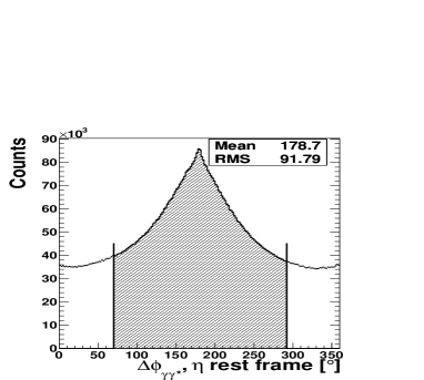
(a) Without particle identification in SEC

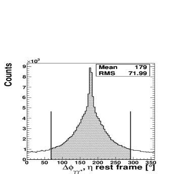
(b) With particle identification in SEC

Fig. 5.7: Experimental distributions of the difference in the azimuthal angle between real and virtual photon $\mathrm{\Delta}\phi_{\gamma\gamma*}$, in the $\mathrm{\displaystyle}\eta$ rest frame. Shaded area corresponds to the window accepted in the analysis.

Multiplicity of neutral particles is shown in Fig. 5.8.

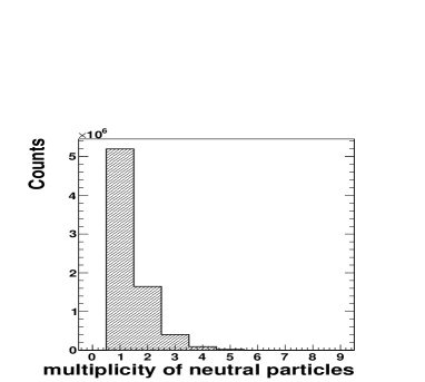
(a) All photon candidates

(b) Photons candidates within $\mathrm{\Delta}\phi_{\gamma\gamma*}$ cut

Fig. 5.8: Multiplicity of candidates for neutral particles.

The initial situation is presented in Fig. 5.8a. Here, the only demand was to have at least one neutral particle in each event. The situation after applying selection cuts described above is depicted in Fig. 5.8b. Most of photons candidates do not fulfill selection criteria. For further analysis, those events, where only one photon matches the $\mathrm{\Delta}\phi_{\gamma\gamma*}$ criteria, are accepted.

5.4 Identification of Leptons

Selection of leptons aims at reducing the background from reactions with charged pions such as the $\mathrm{\displaystyle}\eta\rightarrow\pi^{+}\pi^{-}\gamma$ and the $\mathrm{\displaystyle}\eta\rightarrow\pi^{+}\pi^{-}\pi^{0}\,$.

In the first step, to make sure that tracks from oppositely charged particles, reconstructed in the Central Detector, come from the $\mathrm{\displaystyle}pd\rightarrow{}^{3}He\,\eta\to{}^{3}He\,\gamma\gamma^{*}$
$\mathrm{\displaystyle}\to{}^{3}He\,\gamma\,e^{-}e^{+}$ reaction, they are checked for time coincidences with the $\mathrm{\displaystyle}\,{}^{3}He$ identified in the Forward Detector. Corresponding spectrum is shown in Fig. 5.9. A cut on time difference $\mathrm{\Delta}T$ of [-5,8] ns was chosen.

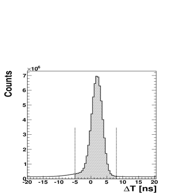
(a) For positively charged particles registered
in the Central Detector

(b) For negatively charged particles registered in the Central Detector

Fig. 5.9: Experimental distribution of the time difference between charged particles in the Central Detector and $\mathrm{\displaystyle}\,{}^{3}He$ ions identified in the Forward Detector. Dashed lines show time cut used in analysis.

The charged particle identification in the Central Detector aims at selecting tracks coming from $\mathrm{e}^{+}$ and $\mathrm{e}^{-}$ particles. For this purpose, correlation between energy deposited in the Scintillating Electromagnetic Calorimeter and particle’s momentum is used. Four densely populated areas are visible in Fig. 5.10. As marked in the picture, they correspond to leptons and pions with opposite charge.

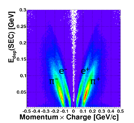
Fig. 5.10: Simulated spectrum of the energy deposited in the calorimeter as a function of the product of particles’ momentum and charge. Lepton bands arrange themselves close to the momentum-$\mathrm{E}_{dep}$ diagonal, while pions, carrying same momentum, have relatively smaller energy and they group below lepton bands.

However, this clear situation is observed in simulations only, where the number of simulated electrons and pions is similar (e.g. in $\mathrm{\eta}\rightarrow e^{+}e^{-}\pi^{+}\pi^{-}$ or $\mathrm{\eta}\rightarrow\pi^{+}\pi^{-}\pi^{0}\rightarrow\pi^{+}\pi^{-}(e^{+}e^{-}\gamma)$ reactions). In the analysis of experimental data, due to the higher number of pions with respect to electrons, pions’ bands are shading electrons’. Such situation is seen even after $\mathrm{\displaystyle}\,{}^{3}He$ and $\mathrm{\displaystyle}\gamma$ selection, when one demands exactly two, oppositely charged particles in the Central Detector correlated in time with the $\mathrm{\displaystyle}\,{}^{3}He$ (see Fig. 5.11a).

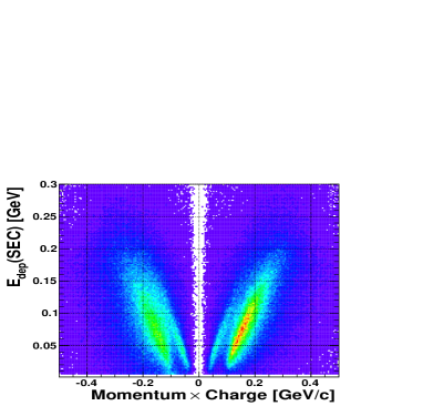
(a) Before restriction on $\mathrm{\Omega}^{+,-}$

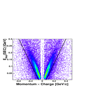
(b) $\mathrm{\Omega}^{+,-}<10^{\circ}$

Fig. 5.11: Experimental spectra which are used to determine the area of leptons’ occurrence. Particles giving input to the region above solid lines shown in (5.11b), are considered as leptons.

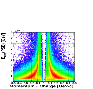
Fig. 5.12: Energy deposited in the Plastic Scintillator Barrel as a function of the product of particles’ momentum and charge from simulations (left) and experiment (right). The experimental spectrum was plotted after applying particle identification based on dependence of the energy deposition in the calorimeter on the particles momenta. Solid lines show the course of the cut.

Therefore, to set up the region within which leptons are located, the identification plot is made with an additional restriction on the opening angle between positively and negatively charged particles $\mathrm{\Omega}^{+,-}$. In the overwhelming majority, leptons from the $\mathrm{\gamma^{*}\rightarrow e^{+}e^{-}}$ conversion create small opening angle [67]. Experimental spectrum in Fig. 5.11b is plotted under condition that $\mathrm{\Omega}^{+,-}$ is less than $\mathrm{1}0^{\circ}$. This allows (on the basis of experimental data) to define the region where leptons are located. It is important to stress, that this restriction is not used in the further analysis.

Particles, identified in the calorimeter as $\mathrm{e}^{+}$ and $\mathrm{e}^{-}$, are further checked, if also in the Plastic Scintillator Barrel their energy losses are as expected for electrons. The simulated spectrum of the energy deposited in the Plastic Scintillator Barrel as a function of the product of particles’ momentum and charge is shown in the left panel of Fig. 5.12. Below pion bands, electrons are forming stripes with almost a constant energy deposit in the whole range of the momentum. The same distribution from experimental data, but containing only particles which fell into the lepton’s region in the calorimeter, is presented in the right panel. Misidentified particles in the Scintillating Electromagnetic Calorimeter are rejected in the Plastic Scintillator Barrel using the cut shown as a solid line in the right panel of Fig. 5.12.

The maximal geometrical acceptance of the Central Detector is $\mathrm{2}0-169$ degrees. Due to the lower granularity of the calorimeter crystals in the back part, and an exit cone in the front part of the Central Detector, the reconstruction of charged particles is worst in these regions. Fig. 5.13

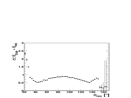
Fig. 5.13: The absolute error (standard deviation) of the leptons’ polar angle reconstruction as a function of the reconstructed polar angle. At higher angles, due to the lower statistics, a good fit was not possible. For this plot $\mathrm{1}0^{6}$ of $\mathrm{\displaystyle}\eta\rightarrow e^{+}e^{-}\gamma$ events has been simulated.

shows the standard deviation of uncertainty of the leptons’ polar angle reconstruction as a function of reconstructed polar angle. A significant worsening of accuracy is observed for small and highest angles. Therefore, it is demanded in the further analysis that leptons were emitted in the range of the polar angle $\mathrm{\theta}$ of $\mathrm{3}0-150$ degrees.

5.5 Selection of the $\mathrm{\displaystyle}\eta\rightarrow e^{+}e^{-}\gamma$

After the particle identification described above, one can plot the distribution of the missing mass for the $\mathrm{p}d\rightarrow{}^{3}HeX$ reaction as a function of the invariant mass of the lepton pairs, $\mathrm{\displaystyle}M_{e^{+}e^{-}}$. This spectrum is shown in Fig. 5.14. The width of intervals of $\mathrm{\displaystyle}M_{e^{+}e^{-}}$ mass was chosen based on the $\mathrm{\displaystyle}M_{e^{+}e^{-}}$ resolution and it is growing with the $\mathrm{\displaystyle}M_{e^{+}e^{-}}$ mass. The corresponding spectrum of generated $\mathrm{M}_{e^{+}e^{-}}^{\text{true}}$ mass as a function of generated and then reconstructed $\mathrm{M}_{e^{+}e^{-}}^{\text{rec}}$ mass is shown in Fig. 5.15. One can see that the reconstruction resolution worsen for higher $\mathrm{\displaystyle}M_{e^{+}e^{-}}$ masses.

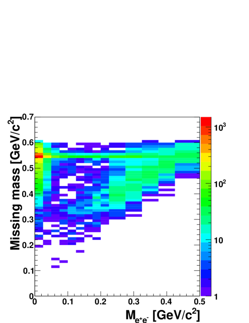
Fig. 5.14: The experimental distribution of the missing mass for the $\mathrm{pd\rightarrow{}^{3}HeX}$ reaction as a function of the invariant mass of the lepton pairs after particle selection described in the previous section.

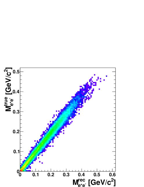
Fig. 5.15: Distribution of generated $\mathrm{M}_{e^{+}e^{-}}^{\text{true}}$ mass as a function of generated and then reconstructed $\mathrm{M}_{e^{+}e^{-}}^{\text{rec}}$ mass of $\mathrm{\displaystyle}e^{+}e^{-}$ pairs.

In Fig. 5.14, an enhancement in the number of entries is visible for the missing mass equal to the mass of the $\mathrm{\displaystyle}\eta$ meson. However, this signal appears on a background caused by reaction in which only helium and pions were produced namely, the $\mathrm{\displaystyle}pd\rightarrow{}^{3}He\,\pi^{+}\pi^{-}$ reaction. In case of this events, the particle identification described in the previous section turned out to be not sufficient. Nevertheless, this background can be well suppressed in the region below the $\mathrm{\displaystyle}\eta$ mass, by a cut on the scattering angle of helium ions, $\mathrm{\theta}_{{}^{3}He}$. It is because in the case of the pion production, the maximal laboratory $\mathrm{\displaystyle}\,{}^{3}He$ scattering angle increases as the missing mass decreases. $\mathrm{\displaystyle}\,{}^{3}He$ particles produced in the $\mathrm{\displaystyle}pd\rightarrow{}^{3}He\,\eta$ reaction at a beam momentum of $\mathrm{1}.7~{}GeV/c$ are emitted up to the $\mathrm{\sim}10^{\circ}$ of the $\mathrm{\displaystyle}\,{}^{3}He$ scattering angle. Setting an upper limit on the $\mathrm{\theta}_{{}^{3}He}$ makes the signal better visible. It is especially useful in the region of higher invariant masses of $\mathrm{\displaystyle}e^{+}e^{-}$ pairs, where the statistics is decreasing. The influence of this cut can be seen by comparing spectra in Fig. 5.14 (before applying this cut) and Fig. 5.16 (after cut application).

Fig. 5.16: The experimental distribution of the missing mass for the $\mathrm{pd\rightarrow{}^{3}HeX}$ reaction as a function of the invariant mass of the lepton pairs after particle selection described in the previous section and after cut on the $\mathrm{\displaystyle}\,{}^{3}He$ scattering angle in laboratory frame ($\mathrm{\theta}_{{}^{3}He}<11^{\circ}$).

Direct production of pions results in a continuous missing mass distribution and can be subtracted from the signal by plotting a missing mass spectrum for each $\mathrm{\displaystyle}e^{+}e^{-}$ invariant mass interval separately. However, the signal on the missing mass spectrum corresponding to the mass of the $\mathrm{\displaystyle}\eta$ meson may be not only due to the investigated $\mathrm{\displaystyle}\eta\rightarrow e^{+}e^{-}\gamma$ decay but also due to the $\mathrm{\displaystyle}\eta\rightarrow\gamma\gamma$, $\mathrm{\displaystyle}\eta\rightarrow\pi^{+}\pi^{-}\gamma$, $\mathrm{\displaystyle}\eta\rightarrow\pi^{+}\pi^{-}\pi^{0}$ and $\mathrm{\displaystyle}\eta\rightarrow 3\pi^{0}\,$  decays. The listed $\mathrm{\displaystyle}\eta$ decays may still contribute to the signal, mainly because of the particle misidentification and the external conversion of photon in the detector material. As it will be shown in Sec. 5.7, almost $\mathrm{3}.5\%$ of the signal content at this stage of the analysis is due to the presence of $\mathrm{\displaystyle}\eta\rightarrow\pi^{+}\pi^{-}\gamma$, $\mathrm{\displaystyle}\eta\rightarrow\pi^{+}\pi^{-}\pi^{0}$ and, especially, $\mathrm{\displaystyle}\eta\rightarrow 3\pi^{0}\,$  decays. The number of $\mathrm{3}.5\%$ is very big since the background events contributing to it, are characterized by higher values of the invariant mass of misidentified leptons pairs and in this region the signal channel has a low cross section. The situation is shown in Fig. 5.17, where the percentage share.

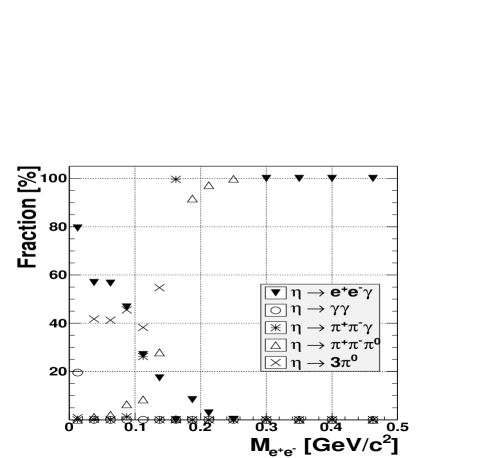
Fig. 5.17: The percentage share of simulated $\mathrm{\displaystyle}\eta$ decay channels as a function of the invariant mass of leptons pairs, plotted after selection described in the previous sections.

In the region of the invariant mass of leptons pairs from $\mathrm{\sim}0.1$ $\mathrm{\text{missing}}{GeV}/c^{2}$ up to $\mathrm{\sim}0.25$ $\mathrm{\text{missing}}{GeV}/c^{2}$, the signal channel is drawn strongly from the events coming from the $\mathrm{\displaystyle}\eta$ decay channels with pions. Below $\mathrm{0}.1$ $\mathrm{\text{missing}}{GeV}/c^{2}$ the background comes mainly from the $\mathrm{\displaystyle}\eta\rightarrow 3\pi^{0}\,$  and $\mathrm{\displaystyle}\eta\rightarrow\gamma\gamma$ decays. In the very small invariant masses of leptons pairs, the $\mathrm{\displaystyle}\eta\rightarrow\gamma\gamma$ decay channel is the dominating background contributor. It is due to the photons conversion at the beam pipe and will be described in Sec. 5.5.2.

Fig. 5.17 shows, that there is essentially no background originating from the $\mathrm{\displaystyle}\eta$ meson decays for $\mathrm{\displaystyle}M_{e^{+}e^{-}}$ invariant masses higher than $\mathrm{0}.3$ $\mathrm{\text{missing}}{GeV}/c^{2}$. In this region, the main background is due to the direct pion production.

5.5.1 Missing Mass for the $\mathrm{p}d\rightarrow X\eta$ Reaction

It is assumed in the analysis, that all charged particles reconstructed in the Central Detector have a mass of electron. Therefore, it is useful to look at the spectrum of the missing mass for the $\mathrm{p}d\rightarrow Xe^{+}e^{-}\gamma$ reaction, calculated as:

$$(M_{X})^{2}c^{4}=(E_{beam}+M_{target}c^{2}-\sum E_{i})^{2}-c^{2}(\vec{p}_{beam}-\sum\vec{p}_{i})^{2},$$ (5.2)

where mass of X should be equal to the mass of the $\mathrm{\displaystyle}\,{}^{3}He$ particle ($\mathrm{M}_{{}^{3}He}=2.809~{}\text{GeV/c}^{2}$), which has been already identified in the Forward Detector, whereas index i runs over particles registered in the Central Detector.

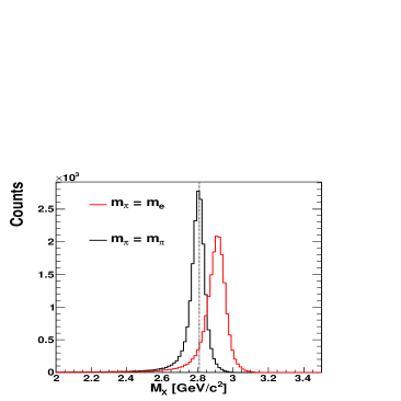
(a) $\mathrm{p}d\rightarrow{}^{3}He\eta\to{}^{3}He\pi^{+}\pi^{-}\gamma$

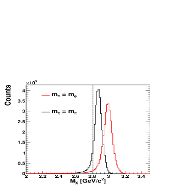
(b) $\mathrm{p}d\rightarrow{}^{3}He\eta\to{}^{3}He\pi^{+}\pi^{-}\pi^{0}$

Fig. 5.18: Simulated missing mass distribution, $\mathrm{M}_{X}$, for two $\mathrm{\displaystyle}\eta$ decay channels. The straight, dashed line shows the $\mathrm{\displaystyle}\,{}^{3}He$ mass, $\mathrm{M}_{{}^{3}He}=2.809~{}\text{GeV/c}^{2}$. The electron’s mass assumption causes spectra shift towards higher masses. In case of the $\mathrm{\displaystyle}\eta\rightarrow\pi^{+}\pi^{-}\pi^{0}$ decay, the shift is even more pronounced since there is, additionally, one photon missing.

If the mass assumption for particles identified as electrons is wrong and pions were misidentified as electrons, the missing mass $\mathrm{M}_{X}$ will not be equal to the mass of the recoil particle. In case of $\mathrm{\displaystyle}\eta$ decays into pions it will be shifted towards higher masses as can be seen in Fig. 5.18. Experimental spectrum of the missing mass, $\mathrm{M}_{X}$ is shown in the right panel of Fig. 5.19.

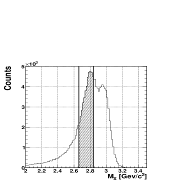
Fig. 5.19: Left: The distribution of the difference between the true and the reconstructed value of the $\mathrm{M}_{X}$. Right: The experimental distribution of the $\mathrm{M}_{X}$ mass. The cut was chosen in the range of $\mathrm{2}.66-2.84$ $\mathrm{\text{missing}}{GeV}/c^{2}$ of $\mathrm{M}_{X}$ as indicated by solid lines.

Broadening of the peak on the right side is caused by the presence of events from such $\mathrm{\displaystyle}\eta$ decay channels like $\mathrm{\displaystyle}\eta\rightarrow 3\pi^{0}\,$ , $\mathrm{\displaystyle}\eta\rightarrow\pi^{+}\pi^{-}\gamma$ and $\mathrm{\displaystyle}\eta\rightarrow\pi^{+}\pi^{-}\pi^{0}$. The range of accepted $\mathrm{M}_{X}$ was chosen from $\mathrm{2}.66$ $\mathrm{\text{missing}}{GeV}/c^{2}$ to $\mathrm{2}.84$ $\mathrm{\text{missing}}{GeV}/c^{2}$. The lower boundary condition was taken as $\mathrm{\sim}(M_{{}^{3}He}-3\sigma)$. In order to estimate the resolution of the $\mathrm{M}_{X}$ determination, the distribution of the difference between true and reconstructed values of the $\mathrm{M}_{X}$ was established. It is shown in the left panel of Fig. 5.19. The upper limit was chosen more restrictively than lower one as $\mathrm{\sim}(M_{{}^{3}He}+1\sigma)$ in order to suppress the background from the $\mathrm{\displaystyle}\eta$ decays into pions.

The influence of the cut on the missing mass for the $\mathrm{p}d\rightarrow Xe^{+}e^{-}\gamma$ reaction is seen in Fig. 5.20. The previously very high contribution of $\mathrm{\displaystyle}\eta\rightarrow\pi^{+}\pi^{-}\gamma$, $\mathrm{\displaystyle}\eta\rightarrow\pi^{+}\pi^{-}\pi^{0}$ and $\mathrm{\displaystyle}\eta\rightarrow 3\pi^{0}\,$  decay channels become insignificant.

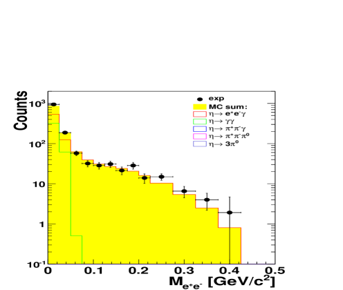
Fig. 5.20: The spectrum of the $\mathrm{\displaystyle}M_{e^{+}e^{-}}$distribution from the experiment (black points) and the simulations (see the legend) after application of the cut on the missing mass for the $\mathrm{p}d\rightarrow Xe^{+}e^{-}\gamma$ reaction.

5.5.2 Photon’s Conversion

Despite of asking in the analysis for events with two oppositely charged particles, there is a large background coming from the $\mathrm{\displaystyle}\eta\rightarrow\gamma\gamma$ decay channel, where only neutral particles are originally produced. It is due to the photons conversion at the beam pipe. In this case, the $\mathrm{\displaystyle}\eta\rightarrow\gamma\gamma$ decay channel has the same signature as the decay of interest. Conversion events contribute strongly to the background in the low invariant mass of leptons pair as it is shown in Fig. 5.17 and 5.20.

Lepton’s pairs, having their origin in the material of the beam pipe, should create there small values of the $\mathrm{M}_{e^{+}e^{-}}^{BP}$. Also, the distance, $\mathrm{R}_{CA}$, between the points, where theirs paths are closest to each other, and the beam line, should be in order of the beam pipe radius. The relevant distribution is shown in Fig. 5.21.

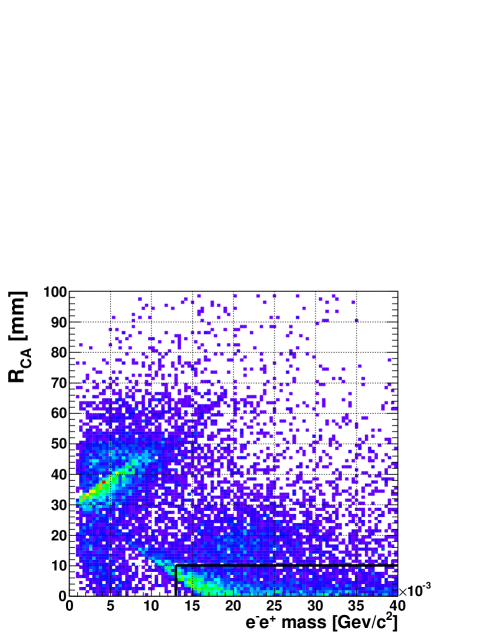
Fig. 5.21: The experimental distribution of the radius of the $\mathrm{\displaystyle}e^{+}e^{-}$ closest approach as a function of the invariant mass of the $\mathrm{\displaystyle}e^{+}e^{-}$ pair calculated assuming that electrons originate from the conversion at the beam pipe.

Conversion events populate the spectrum in the range of low mass, having $\mathrm{R}_{CA}$ above $\mathrm{3}0$ mm. The condition used in the analysis was chosen so, that the $\mathrm{R}_{CA}$ was lower than $\mathrm{1}0~{}$mm while the $\mathrm{M}_{e^{+}e^{-}}^{BP}$, calculated assuming that electrons originate from the conversion at the beam pipe, is higher than $\mathrm{0}.13\times 10^{-3}~{}GeV/c^{2}$.

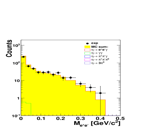
Fig. 5.22: The spectrum of the $\mathrm{\displaystyle}M_{e^{+}e^{-}}$distribution from the experiment (black points) and the simulations (see the legend) after suppression of events originating from the $\mathrm{\gamma}$ conversion at the beam pipe.

In Fig. 5.20 one can see how the conversion influences the $\mathrm{\displaystyle}M_{e^{+}e^{-}}$ distribution. The spectrum is plotted after applying all the other cuts described previously. The green and red lines represent the simulated events of the $\mathrm{\displaystyle}\eta\rightarrow\gamma\gamma$ and $\mathrm{\displaystyle}\eta\rightarrow e^{+}e^{-}\gamma$, respectively. In yellow, the sum of the Monte Carlo generated decays (listed in the legend) is shown. The experimental points are plotted after the subtraction of the background from direct pions production and before efficiency correction. The simulated events of the $\mathrm{\displaystyle}\eta\rightarrow\gamma\gamma$ are entering in the $\mathrm{\displaystyle}M_{e^{+}e^{-}}$ region up to $\mathrm{0}.1$ $\mathrm{\text{missing}}{GeV}/c^{2}$, contributing mostly up to the $\mathrm{\displaystyle}e^{+}e^{-}$ mass of $\mathrm{0}.06$ $\mathrm{\text{missing}}{GeV}/c^{2}$. Fig. 5.22 was plotted with the cut on the distribution of the radius of the closest approach as a function of the $\mathrm{M}_{e^{+}e^{-}}^{BP}$ (see Fig. 5.21) added to the analysis. The $\mathrm{\displaystyle}\eta\rightarrow\gamma\gamma$ input to the signal has been reduced significantly.

Summary of Sec. 5.5

After application of, above described, i) cut on the $\mathrm{\displaystyle}\,{}^{3}He$ scattering angle, ii) the restriction on the missing mass for the $\mathrm{p}d\rightarrow X\eta$ reaction and iii) the suppression of photons conversion at the beam pipe, one obtains the spectrum of the missing mass for the $\mathrm{p}d\rightarrow{}^{3}HeX$ as a function of the invariant mass of leptons pairs, $\mathrm{\displaystyle}M_{e^{+}e^{-}}$, as presented in Fig. 5.23.

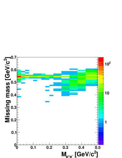
Fig. 5.23: Experimental distribution of the missing mass for the $\mathrm{p}d\to{}^{3}HeX$ reaction as a function of the invariant mass of the $\mathrm{\displaystyle}e^{+}e^{-}$ pair after applying all cuts.

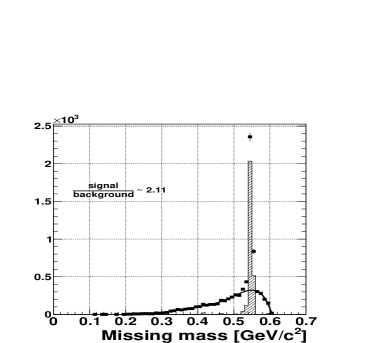
(a) Projection of Fig. 5.14 onto the y-axis

(b) Projection of Fig. 5.23 onto the y-axis

Fig. 5.24: Experimental distributions of the missing mass for the $\mathrm{p}d\to{}^{3}HeX$ reaction. Solid lines show the fit of the 5th order polynomial to the continuous pion background consisting of $\mathrm{\displaystyle}pd\rightarrow{}^{3}He\,\pi^{+}\pi^{-}$ and $\mathrm{\displaystyle}pd\rightarrow{}^{3}He\,\pi^{+}\pi^{-}\pi^{0}$ reactions. Dashed histograms correspond to data after subtraction of this background.

It can be compared to Fig. 5.14 which shows the situation before applying above mentioned conditions. One can notice that the signal become more clear and that there is also less contribution from the $\mathrm{\displaystyle}pd\rightarrow{}^{3}He\,\pi^{+}\pi^{-}$ reaction. Corresponding missing mass spectra for the $\mathrm{p}d\to{}^{3}HeX$ reaction are shown in Fig. 5.24. The signal to background ratio has increased by $\mathrm{\sim}60\%$.

5.6 Consistency Check

It is necessary to check identification criteria after applying all the other cuts and to prove whether the areas of the occurrence of leptons on the identification plots were chosen properly. In the left panel of Fig. 5.25 the experimental distribution of the energy deposited in the Scintillating Electromagnetic Calorimeter as a function of the momentum is shown.

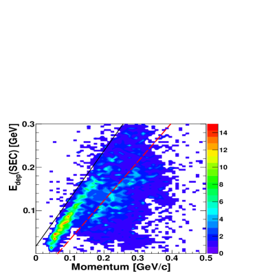
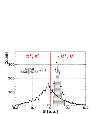
Fig. 5.25: Left : experimental distribution of the energy deposited in the Scintillating Electromagnetic Calorimeter as a function of the momentum. Right: experimental spectrum of the shortest distance, S, between points and the red line shown on the left plot. Points on the left side of the red line are assigned to the positive value of S and these on the right side to negative. The red line indicates the zero position. The black line indicates the fit of the 4th order polynomial function to the background and the dashed histogram is the signal after the background subtraction.

Plot was made after applying conditions described in previous sections (only identification in the Scintillating Electromagnetic Calorimeter was omitted). Additionally, only for the purpose of this check, in order to suppress contribution from direct pion production, cut on the missing mass was applied. The missing mass for the $\mathrm{p}d\rightarrow{}^{3}HeX$ reaction was restricted to the range from $\mathrm{0}.535$ to $\mathrm{0}.56$ $\mathrm{\text{missing}}{GeV}/c^{2}$ (see Fig. 5.24).

The shortest distance from each point on the spectrum to the solid line, is presented in the right panel of Fig. 5.25. The peak centered at about $\mathrm{0}.04$ corresponds to the leptons. In order to estimate the amount of misidentified pions, the signal to background ratio was calculated in the range of $\mathrm{S}\in[0.008;0.08]$, with a resulting value of $\mathrm{\sim}1.8$.

5.7 Estimation of the Background Contribution

To estimate the quality of the background suppression, a set of reactions have been simulated and studied. They are listed in Tab. 5.1, in the second column of which, the number of generated and analyzed events is given.

Simulated background channels	Number of generated
	events $\mathrm{\,}\times\,10^{6}$
$\mathrm{\displaystyle}pd\to{}^{3}He\,\eta\to{}^{3}He\,\gamma\gamma$	50
$\mathrm{\displaystyle}pd\to{}^{3}He\,\eta\to{}^{3}He\,3\pi^{0}\to{}^{3}He\,6\gamma$	43
$\mathrm{\displaystyle}pd\to{}^{3}He\,\eta\to{}^{3}He\,\pi^{+}\pi^{-}\pi^{0}\to{}^{3}He\,\pi^{+}\pi^{-}\gamma\gamma$	30
$\mathrm{\displaystyle}pd\to{}^{3}He\,\eta\to{}^{3}He\,\pi^{+}\pi^{-}\gamma$	7

Table 5.1: A list of reactions which have been simulated and studied as a background for the $\mathrm{\displaystyle}pd\rightarrow{}^{3}He\,\eta\to{}^{3}He\,\gamma\,e^{-}e^{+}$ reaction. The relative number of generated events corresponds very roughly to the ratios of branching ratios of the studied channels (see Tab. 1.1).

Each of $\mathrm{\displaystyle}\eta$ decays may cause a signal contamination.

First, a study of the efficiency for the reconstruction of the $\mathrm{\displaystyle}\eta$ decay channels under different conditions had been made as shown in Fig. 5.26. The cuts were added subsequently to the analysis, one after the other, and the calculated percentages of events left, were plotted in corresponding bins named after

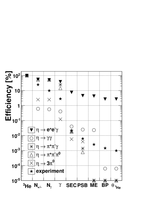
Explanation of the x-axis abbreviations:
gray!40 $\mathrm{}^{3}He$	selection of the $\mathrm{\displaystyle}\,{}^{3}He$ in the Forward Detector,		described in Sec. 4.3
gray!40	time correlations between particles registered in the Central Detector and in the Forward Detector		see Fig. 5.9 and Fig. 5.4
$\mathrm{N}_{+/-}$	reconstruction of tracks corresponding to two particles with opposite charges
gray!40 $\mathrm{N}_{\gamma}$	requirement of at least one neutral particle with $\mathrm{E>0.02}$ GeV
$\mathrm{\gamma}$	selection of the photon		described in Sec. 5.3
gray!40 $\mathrm{S}EC$	particle identification using the Scintillating Electromagnetic Calorimeter		see Fig. 5.25
$\mathrm{P}SB$	particle identification using the Plastic Scintillator Barrel		see Fig. 5.12
gray!40 $\mathrm{M}E$	cut on the missing mass for the $\mathrm{pd\rightarrow X\eta}$ reaction		[2.66,2.84] GeV
$\mathrm{B}P$	suppression of photons conversion		see Fig. 5.21
gray!40 $\mathrm{\theta}_{{}^{3}He}$	cut on the scattering angle of the $\mathrm{\displaystyle}\,{}^{3}He$		$\mathrm{\theta}_{{}^{3}He}<11^{\circ}$

Fig. 5.26: Reconstruction efficiency for different $\mathrm{\displaystyle}\eta$ decay channels after applying subsequent cuts.

the last added condition. The abbreviations used to describe the x-axis are explained below the plot. The last condition on the $\mathrm{\displaystyle}\,{}^{3}He$ scattering angle is used for the reduction of the background from the direct pions production and here it is plotted to check if it doesn’t influence the $\mathrm{\displaystyle}\eta$ decay channels. After applying all conditions, the final efficiency for the $\mathrm{\displaystyle}\eta\rightarrow e^{+}e^{-}\gamma$ decay is equal to $\mathrm{\sim}2.7\%$ while for the background channels the efficiency is negligible. A non-zero efficiency is noted for the $\mathrm{\displaystyle}\eta\rightarrow\gamma\gamma$ and $\mathrm{\displaystyle}\eta\rightarrow 3\pi^{0}\,$  decay channels only.

One can notice that the efficiency for the signal channel decreases suddenly after application of the identification in the Scintillating Electromagnetic Calorimeter. There is however no damage in the percentage share of this channel, in the total number of $\mathrm{\displaystyle}\eta$ mesons, shown in the Fig. 5.27.

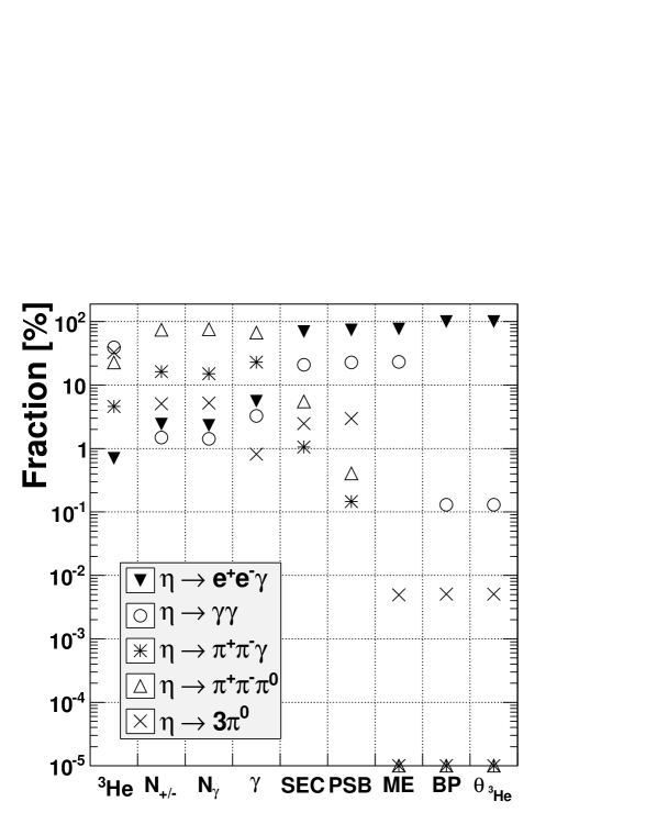
Fig. 5.27: Percentage share of different $\mathrm{\displaystyle}\eta$ decay channels in the total number of reconstructed $\mathrm{\displaystyle}\eta\rightarrow e^{+}e^{-}\gamma$ events after applying subsequent cuts, obtained from the simulations. The cuts abbreviations are given in Fig. 5.26.

Moreover, a constant increase in the amount of the $\mathrm{\displaystyle}\eta\rightarrow e^{+}e^{-}\gamma$ events in the relation to other channels is observed.

After applying in the analysis all conditions described above, almost $\mathrm{1}00\%$ of all events, reconstructed from studied $\mathrm{\displaystyle}\eta$ decay channels, come from the $\mathrm{\displaystyle}\eta\rightarrow e^{+}e^{-}\gamma$ channel and the only significant background, comes from the direct $\mathrm{\pi}$ meson production. This background creates a continuous shape over a wide range of the missing mass for the $\mathrm{p}d\to{}^{3}HeX$ reaction and can be easily subtracted using a polynomial function as was shown in Fig. 5.24.

Chapter 6 Results

6.1 Calculation of the Transition Form Factor

The final spectrum of the missing mass for the $\mathrm{p}d\to{}^{3}HeX$ reaction as a function of the invariant mass of the $\mathrm{\displaystyle}e^{+}e^{-}$ pair is shown in Fig. 6.1.

Fig. 6.1: Experimental distribution of the missing mass for the $\mathrm{p}d\to{}^{3}HeX$ reaction as a function of the invariant mass of the $\mathrm{\displaystyle}e^{+}e^{-}$ pair after applying event selection described in previous chapters.

Counts $\mathrm{\xrightarrow{missing}}{\hskip 512.1496pt}$
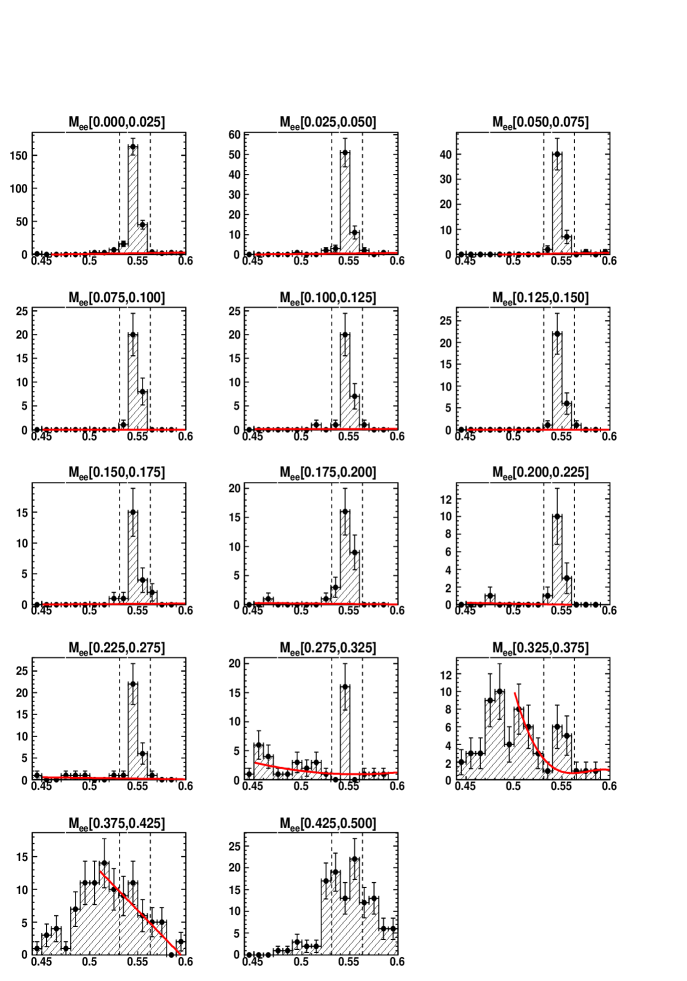
$\mathrm{\xrightarrow{missing}}{\hskip 355.65944pt}$
Missing mass [$\mathrm{G}eV/c^{2}$]

Fig. 6.2: Experimental distributions of the missing mass for the $\mathrm{p}d\to{}^{3}HeX$ reaction for fourteen $\mathrm{\displaystyle}M_{e^{+}e^{-}}$ intervals ( x-bins of the distribution shown in Fig. 6.1 ). With dashed lines, the signal region is marked.

In order to subtract the background coming from direct pion production, the missing mass for the $\mathrm{p}d\to{}^{3}HeX$ reaction was determined for each $\mathrm{\displaystyle}M_{e^{+}e^{-}}$ interval separately. The result is shown in Fig. 6.2.

The background was fitted with the first order polynomial, omitting the signal region of $\mathrm{[0.531,0.563]}$ $\mathrm{\text{missing}}{GeV}/c^{2}$. In the region of $\mathrm{\displaystyle}M_{e^{+}e^{-}}$$\mathrm{\in}{[0.275,0.375]}$ $\mathrm{\text{missing}}{GeV}/c^{2}$ the background is not flat and was fitted with a higher order polynomial. In the range of $\mathrm{\displaystyle}M_{e^{+}e^{-}}$ from $\mathrm{0}.425$ $\mathrm{\text{missing}}{GeV}/c^{2}$ to $\mathrm{0}.500$ $\mathrm{\text{missing}}{GeV}/c^{2}$ no signal is observed. Therefore, this interval of $\mathrm{\displaystyle}M_{e^{+}e^{-}}$ has been excluded from further analysis.

The $\mathrm{\displaystyle}M_{e^{+}e^{-}}$ distribution, plotted after the background subtraction is shown in Fig. 6.3. The obtained number of $\mathrm{\displaystyle}\eta\rightarrow e^{+}e^{-}\gamma$ events amounts to $\mathrm{5}25\pm 26$.

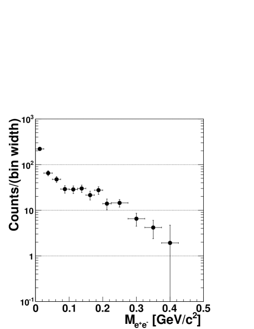
Fig. 6.3: Experimental spectrum of the $\mathrm{\displaystyle}M_{e^{+}e^{-}}$ distribution after the background subtraction.

In the next step, the $\mathrm{\displaystyle}M_{e^{+}e^{-}}$ distribution was corrected for the reconstruction efficiency. Efficiences, calculated per bin of the $\mathrm{\displaystyle}M_{e^{+}e^{-}}$, consist of the trigger efficiency, the reconstruction and selection efficiencies and the geometrical acceptance. The efficiency as a function of the Mee is shown in Fig. 6.4. Each of the $\mathrm{\displaystyle}M_{e^{+}e^{-}}$ bin content was divided by the corresponding value of the efficiency. The outcome of this operation is presented in Fig. 6.5.

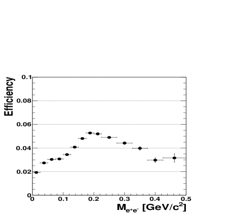
Fig. 6.4: The efficiency for the reconstruction of the $\mathrm{\displaystyle}pd\rightarrow{}^{3}He\,\eta\to{}^{3}He\,\gamma\gamma^{*}\to{}^{3}He\,\gamma\,e^{-}e^{+}$ reaction as a function of the invariant mass of leptons pairs, $\mathrm{\displaystyle}M_{e^{+}e^{-}}$.

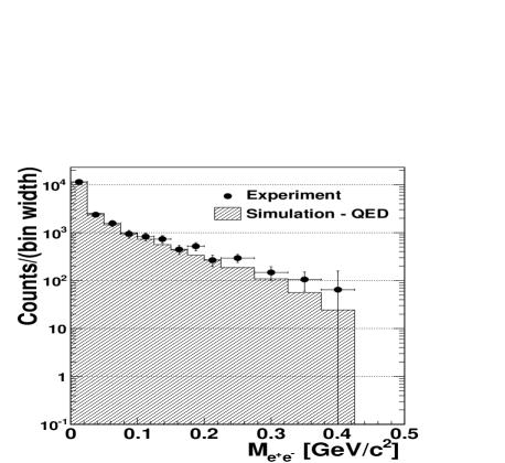
Fig. 6.5: Experimental spectrum of the $\mathrm{\displaystyle}M_{e^{+}e^{-}}$ distribution after background subtraction, efficiency corrected. Filled histogram corresponds to efficiency corrected data, simulated with the transition form factor equal to one.

In order to obtain the transition form factor, experimental data points were divided by the Monte Carlo data, simulated with the transition form factor equal to one. The QED model assumption of a point-like meson, superimposed over the experimental spectrum is shown in Fig. 6.5. It was normalized to the experimental data points using the $\mathrm{\chi}^{2}$ method. The resulting distribution of the transition form factor squared, $\mathrm{|}F_{\eta}|^{2}$, as a function of the invariant mass of the leptons pairs, $\mathrm{\displaystyle}M_{e^{+}e^{-}}$ is shown in Fig. 6.6.

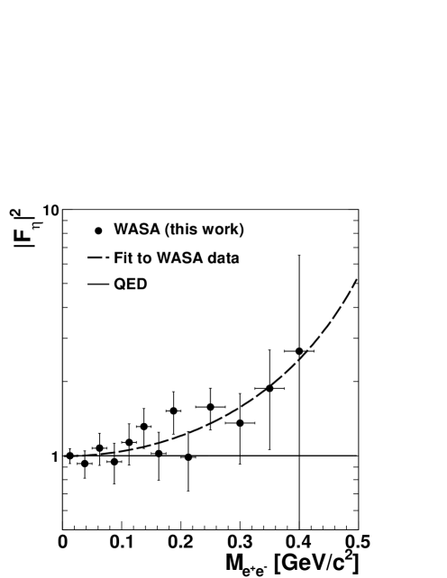
Fig. 6.6: Experimental spectrum of the squared transition form factor, $\mathrm{|}F_{\eta}|^{2}$, as a function of the $\mathrm{\displaystyle}M_{e^{+}e^{-}}$. The dashed line is the result of the fit of the single-pole formula to experimental points with $\mathrm{\chi}^{2}/NDF=0.43$. The solid line is the QED model assumption of a point-like meson.

The experimental data points were fitted with the single-pole formula:

$$\left[F_{P}(q^{2})\right]^{2}=\left[\alpha\left(1-\frac{q^{2}}{\Lambda_{P}^{2}}\right)^{-1}\right]^{2}.$$ (6.1)

The extracted value of the normalization parameter $\mathrm{\alpha}$ is $\mathrm{0}.998\pm 0.025$ whereas the fit parameter $\mathrm{\Lambda}_{P}$ amounted to $\mathrm{(}0.66\pm 0.11)$ GeV. Therefore the slope parameter $\mathrm{b}_{P}\equiv 1/\Lambda_{P}^{2}$ is

$${\Large\displaystyle 2.27\pm 0.73}~{}\frac{\displaystyle 1}{\displaystyle\text{GeV}^{2}}.$$

6.2 Estimation of the Systematic Uncertainty

To estimate the systematic uncertainty, the slope parameter, $\mathrm{\it b_{P}}$, has been re-evaluated changing the initial condition of each selection criteria separately. The systematic error evaluation was done in two ways. First, the systematic error, $\mathrm{\sigma}_{syst}$, was calculated as the square root of the quadratic sum of all contributions:

$$\sigma_{syst}=\sqrt{\sum(x_{i}-x_{r})^{2}},$$ (6.2)

where $\mathrm{\it x_{i}}$ is the result obtained by analyzing data with change in the cut condition and $\mathrm{\it x_{r}=\text{2.27}}$ $\mathrm{\text{missing}}{GeV}^{-2}$ is the result obtained in the previous section. The second evaluation of the systematic uncertainty was done based on the method described in [68] and recommended by the WASA-at-COSY collaboration.

1. Identification of charged particles (SEC)

   Charged particles are identified based on the energy deposited in the Scintillating Electromagnetic Calorimeter plotted as a function of the momentum. The relative distribution is shown in the left panel of Fig. 5.25 (page 5.25). A pair of charged particles is treated as leptons if both of them fall into the area limited by the cut lines. Lines can be parametrized by a function $\mathrm{f(E_{dep})={\it A}\times Momentum+{\it B}}$. In order to estimate the influence of the identification of leptons, the red, dashed line visible in Fig. 5.25, which separates pions from electrons, was moved closer to leptons by change of the B parameter. The allowed area was decreased by $\mathrm{5}\%$. The obtained value of the slope parameter $\mathrm{\it b_{P}}$ is $\mathrm{2}.03$ $\mathrm{\text{missing}}{GeV}^{-2}$. The corresponding transition form factor distribution is shown in the left panel of Fig. 6.7.

   

   

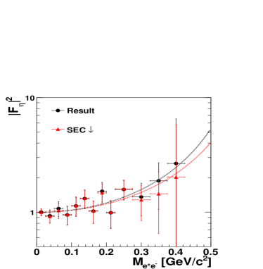
   Fig. 6.7: Experimental spectra of the transition form factor as a function of the invariant mass of $\mathrm{\displaystyle}e^{+}e^{-}$ pairs. The distribution obtained in Sec. 6.1 (black points) is shown in comparison to distribution obtained by changing the condition on the particle identification in the Scintillating Electromagnetic Calorimeter (left) and in the Plastic Scintillator Barrel (right) as it is described in the text. Additionally, results of two corresponding fits are plotted.

2. Identification of charged particles (PSB)

   The additional method to distinguish between pions and leptons in the Central Detector is to use the dependency of energy deposited in the Plastic Scintillator Barrel from particles momenta (see Fig. 5.12, page 5.12). The originally accepted area shown in this figure was decreased by $\mathrm{5}\%$ via the change of the angle of inclination of a cut line. The resulting value of the slope parameter is $\mathrm{\it b_{P}}$ = $\mathrm{2}.31$ $\mathrm{\text{missing}}{GeV}^{-2}$. The corresponding form factor distribution is shown in the right panel of Fig. 6.7.

3. Cut on the missing mass for the $\mathrm{p}d\rightarrow X\eta$ reaction, $\mathrm{M}_{X}$

   The cut used in the analysis can be seen in Fig. 5.19 (page 5.19). In order to estimate the influence of this cut on the final result, the allowed window was increased by $\mathrm{5}\%$ and the analysis was repeated. The obtained value of the slope parameter amounted to $\mathrm{\it b_{P}}$ = $\mathrm{2}.02$ $\mathrm{\text{missing}}{GeV}^{-2}$. The corresponding transition form factor distribution is shown in the left panel of Fig. 6.8.

   

   

   Fig. 6.8: Experimental spectra of the transition form factor as a function of the invariant mass of $\mathrm{\displaystyle}e^{+}e^{-}$ pairs. The distribution obtained in Sec. 6.1 (black points) is shown in comparison to distribution obtained by changing the condition on the missing mass for the $\mathrm{p}d\rightarrow X\eta$ reaction (left) and on the angle between neutral and closest charged particle (right) as it is described in the text. Additionally, results of two corresponding fits are plotted.

4. Cut on the angle between neutral and closest charged particle, $\mathrm{\Omega}$

   In the analysis the minimal accepted angle $\mathrm{\Omega}$ amounts to $\mathrm{6}0^{\circ}$ as depicted in Fig. 5.5 (page 5.5). The analysis was done also for the minimal $\mathrm{\Omega}$ angle increased by $\mathrm{5}\%$ resulting in the slope parameter $\mathrm{\it b_{P}}$ = $\mathrm{2}.37$ $\mathrm{\text{missing}}{GeV}^{-2}$. The corresponding transition form factor distribution is shown in the right panel of Fig. 6.8.

5. Cut suppressing photons conversion

   For the condition used in the analysis to minimize number of conversion events, the allowed area (see Fig. 5.21, page 5.21) was increased by $\mathrm{5}\%$. The resulting value of the slope parameter amounted to $\mathrm{\it b_{P}}$ $\mathrm{=}2.24$ $\mathrm{\text{missing}}{GeV}^{-2}$.

6. Cut on the opening angle between virtual and real photon in the $\mathrm{\displaystyle}\eta$ rest frame, $\mathrm{\Delta}\phi_{\gamma\gamma*}$

   The $\mathrm{\Delta}\phi_{\gamma\gamma*}$ distributions are shown in Fig. 5.7 (page 5.7). The original restriction of $\mathrm{\Delta}\phi_{\gamma\gamma*}$ being in the range of $\mathrm{[}70,290]$ degrees seems quite loose and might give an impression that many right events are rejected due to the presence of fake signals caused by detector’s noise and split-offs. To check that, the accepted cut window was decreased symmetrically by $\mathrm{2}0\%$ via change of the allowed range to $\mathrm{[}92,268]$ degrees. The resulting slope parameter $\mathrm{\it b_{P}}$ amounts to $\mathrm{2}.41$ $\mathrm{\text{missing}}{GeV}^{-2}$. Its deviation from the original result is small relative to the change of the cut made in this test. It implicates that effects caused by fake signals have been already suppressed by former restrictions, especially by the cut on the photons energy as a function of the angle between the neutral and the closest charged particle, $\mathrm{E}_{\gamma}(\Omega$).

7. Cut on photons energy, $\mathrm{E}_{\gamma}(\Omega)$

   Cut on photons energy is shown in the same Fig. 5.5. The minimal photons energy is chosen as a function of the angle between neutral and closest charged particle, $\mathrm{\Omega}$. The influence of this condition on the final result was studied via decrease of accepted area as shown in the left panel of Fig. 6.9. The resulting value of the slope parameter amounted to $\mathrm{\it b_{P}}$ = $\mathrm{2}.33$ $\mathrm{\text{missing}}{GeV}^{-2}$. The corresponding transition form factor distribution is shown in the right panel of Fig. 6.9.

   

   

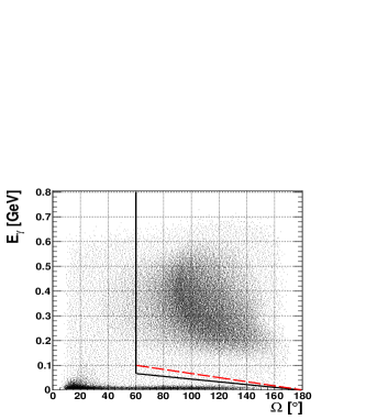
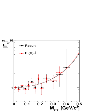
   Fig. 6.9: Left: Simulated spectrum of cluster’s energy vs. the angle it creates with the nearest track for the $\mathrm{\displaystyle}pd\rightarrow{}^{3}He\,\eta\to{}^{3}He\,\gamma\,e^{-}e^{+}$ reaction. The red, dashed line shows the new position of the original cut marked by the solid, black line. Right: Experimental spectrum of the transition form factor as a function of the invariant mass of $\mathrm{\displaystyle}e^{+}e^{-}$ pairs. The distribution obtained in Sec. 6.1 (black points) is shown in comparison to distribution obtained by changing the condition on the $\mathrm{E}_{\gamma}(\Omega)$ as described in the text. Additionally, results of two corresponding fits are plotted.

8. Shape of the multipion background

   The direct production of pions results in a continuous missing mass distribution. It can be described with a polynomial function and subtracted from the signal. In order to check how the choice of the fitting function influences the result, the order of the given polynomial was changed and the slope parameter was recalculated. The resulting value is $\mathrm{\it b_{P}}$ = $\mathrm{2}.33$ $\mathrm{\text{missing}}{GeV}^{-2}$.

9. Size of the $\mathrm{\displaystyle}M_{e^{+}e^{-}}$ bin intervals

   In order to check how the change of the binning of the $\mathrm{\displaystyle}M_{e^{+}e^{-}}$ distribution changes the result, the size of the $\mathrm{\displaystyle}M_{e^{+}e^{-}}$ bin intervals was set to $\mathrm{0}.04$ MeV and the full analysis including multipion background subtraction was repeated. With this new binning, the obtained value of the slope parameter amounted to $\mathrm{\it b_{P}}$ = $\mathrm{2}.04$ $\mathrm{\text{missing}}{GeV}^{-2}$.

Summary

The results of analyses are gathered in Tab. 6.1. In the last column, the difference between the result presented in the previous section and the value obtained with a different cut condition, is shown.

Cut	$\mathrm{\it b_{P}}$[ $\mathrm{\text{missing}}{GeV}^{-2}$]	$\mathrm{\Delta}$$\mathrm{\it b_{P}}$[ $\mathrm{\text{missing}}{GeV}^{-2}$]
	($\mathrm{\it x_{i}}$)	$\mathrm{|}{\it x_{i}-x_{r}}|$
Identification in the SEC	$\mathrm{2}.03$	0.24
Identification in the PSB	$\mathrm{2}.31$	0.04
Missing mass for the $\mathrm{p}d\rightarrow X\eta$ reaction	$\mathrm{2}.02$	0.25
$\mathrm{\Omega}$	$\mathrm{2}.37$	0.10
Photons conversion	$\mathrm{2}.27$	0.00
$\mathrm{\Delta}\phi_{\gamma\gamma*}$	$\mathrm{2}.41$	0.14
$\mathrm{E}_{\gamma}(\Omega$)	$\mathrm{2}.33$	0.06
Shape of the multipion background	$\mathrm{2}.33$	0.06
$\mathrm{\displaystyle}M_{e^{+}e^{-}}$ intervals size	$\mathrm{2}.04$	0.23

Table 6.1: Values of the slope parameter, $\mathrm{\it b_{P}}$, obtained as a result of analyses performed after change in a given cut parameter. Details are given in the text.

The value of the systematic uncertainty calculated using Eq. 6.2 amounts to:

$$\sigma_{syst}=0.46~{}\text{GeV}^{-2}.$$

It is important to stress that all obtained values of systematic uncertainty agree within one standard deviation of the statistical uncertainty. Therefore, this preliminary estimation of the systematic error can be treated as conservative taking into account performed tests.

In order to evaluate the systematic uncertainty as described in [68], the deviation of the original result from the one obtained after the change, denoted as $\mathrm{\Delta}$$\mathrm{\it b_{P}}$, is compared with $\mathrm{\Delta}\sigma$, defined as:

$$\Delta\sigma=\sqrt{\sigma_{r}^{2}-\sigma_{i}^{2}},$$ (6.3)

where $\mathrm{\sigma}_{r}$ and $\mathrm{\sigma}_{i}$ denote statistical uncertainties of the $\mathrm{x}_{r}$ and $\mathrm{x}_{i}$ determinations respectively.

	$\mathrm{\it b_{P}}$	$\mathrm{\sigma}$	$\mathrm{\Delta}$$\mathrm{\it b_{P}}$	$\mathrm{\Delta}\sigma$	$\mathrm{\frac{missing}{missing}}{\Delta b_{P}}{\Delta\sigma}$
Result obtained in Sec. 6.1	2.27	0.73
Cut
Identification in the SEC	$\mathrm{2}.03$	0.78	0.24	0.27	0.87
Identification in the PSB	$\mathrm{2}.31$	0.72	0.04	0.12	0.33
Missing mass for the $\mathrm{p}d\rightarrow X\eta$ reaction	$\mathrm{2}.02$	0.78	0.25	0.27	0.91
$\mathrm{\Omega}$	$\mathrm{2}.37$	0.74	0.10	0.12	0.82
Photons conversion	$\mathrm{2}.27$	0.73	0.00	0.00	0.00
$\mathrm{\Delta}\phi_{\gamma\gamma*}$	$\mathrm{2}.41$	0.69	0.14	0.24	0.59
$\mathrm{E}_{\gamma}(\Omega$)	$\mathrm{2}.33$	0.71	0.06	0.17	0.35
Shape of the multipion background	$\mathrm{2}.33$	0.75	0.06	0.17	0.35
$\mathrm{\displaystyle}M_{e^{+}e^{-}}$ intervals size	$\mathrm{2}.04$	0.81	0.23	0.35	0.66

Table 6.2: Values of the slope parameter, $\mathrm{\it b_{P}}$, obtained as a result of analyses performed after change in a given cut parameters. Details are given in the text.

Tab. 6.2 summarizes the results of performed systematic checks for the slope parameter $\mathrm{\it b_{P}}$, their deviations from the original result, $\mathrm{\Delta}$$\mathrm{\it b_{P}}$, and their correlations $\mathrm{\Delta}$$\mathrm{\it b_{P}}$$\mathrm{/}\Delta\sigma$. All performed checks give a non-significant deviation which manifest itself in $\mathrm{\Delta}$$\mathrm{\it b_{P}}$$\mathrm{/}\Delta\sigma$ less than one. This indicates that the systematic error can be neglected.

To sum up foregoing tests, the upper limit of the systematic uncertainty evaluation can be accepted as $\mathrm{\sigma}_{syst}=0.46~{}\text{GeV}^{-2}$ which is less than the statistical error $\mathrm{\sigma}_{stat}=0.73~{}\text{GeV}^{-2}$ obtained in Sec. 6.1. It should be also noted, that although as many as nine possible sources of systematic effects have been tested, there are still checks which may be done in further studies. These are e.g. checks for the possible systematic effects resulting from the accepted uncertainty of the $\mathrm{\displaystyle}M_{e^{+}e^{-}}$ efficiency.

6.3 Charge Radius of the $\mathrm{\displaystyle}\eta$ Meson

Having the slope parameter of the $\mathrm{\displaystyle}\eta$ meson, one can attempt to evaluate its charge radius. The charge distribution is related to the form factor by the Fourier transform

$$F(q^{2})=\int d^{3}r\rho({\bf r})e^{-i{\bf q}\cdot{\bf r}}\simeq 1-\frac{q^{2}}{6}<r^{2}>+...,$$ (6.4)

where $\mathrm{<}r^{2}>/6=b_{P}$. In order to obtain the charge radius of the $\mathrm{\displaystyle}\eta$ meson, the most recent measurements of the $\mathrm{\displaystyle}\eta$ transition form factor (this work, [29] and [31]) have been gathered in Fig. 6.10 and fitted with the single-pole formula given by Eq. 6.1 in the range of $\mathrm{M}_{l^{+}l^{-}}$ from $\mathrm{0}.$ $\mathrm{\text{missing}}{GeV}/c^{2}$ to $\mathrm{0}.48$ $\mathrm{\text{missing}}{GeV}/c^{2}$.

Fig. 6.10: Experimental spectrum of the squared transition form factor, $\mathrm{|}F_{\eta}|^{2}$, as a function of the $\mathrm{M}_{l^{+}l^{-}}$. The green, solid line is the fit to all experimental points. The black, solid line is the QED model assumption of a point-like meson.

The obtained value of the slope parameter amounts to

$${\displaystyle 1.97\pm 0.09}~{}\frac{\displaystyle 1}{\displaystyle\text{GeV}^{2}}$$

and therefore, the charge radius of the $\mathrm{\displaystyle}\eta$ meson is equal to

$${<r_{\eta}^{2}>^{1/2}=0.68\pm 0.02~{}{\text{fm}}}.$$

Theoretical calculations within the framework of the VMD model (See Tab. 1.2) give the value of the charge radius $\mathrm{<}r_{\eta}^{2}>^{1/2}=0.64$ fm, which deviates from the experimental one, by more than two standard deviations.

Interestingly, similar situation has been already observed for pion. Precise calculations based on the chiral perturbation theory and data, give the radius of the pion meson equal to $\mathrm{<}r_{\pi}^{2}>^{1/2}=(0.672\pm 0.010)$ fm [69] while the measurement at MAMI-II led to the pion radius of $\mathrm{<}r_{\pi}^{2}>^{1/2}=(0.74\pm 0.03)$ fm [70]. The discrepancy is in the order of two standard deviation and to minimize it, it was proposed in [71] to include corrections to the pion loops at the order where the radius appears.

Also in the case of a proton, the recently obtained result by Pohl et al. [72], $\mathrm{<r_{P}^{2}>^{1/2}=(0.84184\pm 0.00067)}$ fm, is five standard deviations away from the one of the CODATA compilation of physical constants, $\mathrm{<}r_{P}^{2}>^{1/2}=(0.8768\pm 0.0069)$ fm [73]. The CODATA values of the radius of the proton are determined via the Lamb shift in electronic [73] hydrogen and via unpolarized [74] and polarized [75] electron scattering. The discrepancy between the CODATA and the value extracted using the Lamb shift method in muonic [72] hydrogen is under a world-wide discussion with a tendency to see the cause of the problem in a not sufficiently exact QED calculations [76].

Chapter 7 Summary and Outlook

At the turn of October and November 2008, the WASA-at-COSY collaboration performed an experiment to collect data on the $\mathrm{\displaystyle}\eta$ meson production and decays via the $\mathrm{\displaystyle}pd\rightarrow{}^{3}He\,\eta$ reaction. The COSY facility provided a proton beam of momentum $\mathrm{1}.7$ GeV/c which has been used to produce $\mathrm{\displaystyle}\eta$ mesons by collisions with deuteron target. Decay products of short-lived meson were registered in the central part of the WASA detector and $\mathrm{\displaystyle}\,{}^{3}He$ ions in the forward part. In this work, the conversion decay $\mathrm{\displaystyle}\eta\rightarrow e^{+}e^{-}\gamma$ has been investigated. It is a very interesting decay since the two electrons in the final state come from the conversion of a virtual $\mathrm{\gamma}$ quantum and, therefore, they constitute a rich source of knowledge about the electromagnetic structure of decaying meson. It is a very important feature of this decay process since the $\mathrm{\displaystyle}\eta$ meson is a short-lived neutral particle and it is not possible to investigate its structure via the classical method of particle scattering.

The performed analysis allowed for the extraction of the $\mathrm{\displaystyle}\eta$ transition form factor as a function of the $\mathrm{\displaystyle}e^{+}e^{-}$ mass and, therefore, for the calculation of the slope parameter, related to the charge radius of the $\mathrm{\displaystyle}\eta$ meson.

$\mathrm{5}25\pm 26$ events of the $\mathrm{\displaystyle}\eta\rightarrow e^{+}e^{-}\gamma$ decay channel were reconstructed. The applied restrictions allowed to suppress the background from the other $\mathrm{\displaystyle}\eta$ decays to a negligible level and the multipion background was subtracted from the signal, based on missing mass distributions. The analysis chain led to the determination of the value of the slope parameter, $\mathrm{\it b_{P}}$, equal to ($\mathrm{2.27\pm 0.73_{\text{stat.}}\pm 0.46_{\text{sys.}}}$) $\mathrm{\text{missing}}{GeV}^{-2}$, where the systematical uncertainty should be treated as an upper limit only [68]. This result is consistent with the one obtained by the CB/TAPS collaboration, ($\mathrm{1}.92\pm 0.35_{\text{stat.}}\pm 0.13_{\text{sys.}}$) $\mathrm{\text{missing}}{GeV}^{-2}$ [29]. Distributions of the transition form factor as a function of the $\mathrm{M}_{e^{+}e^{-}}$ mass extracted in both experiments are shown in the left panel of Fig. 7.1.

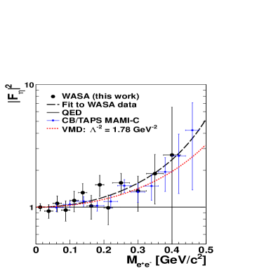
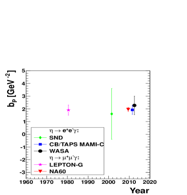
Fig. 7.1: Left : Experimental spectrum of the squared transition form factor, $\mathrm{|}F_{\eta}|^{2}$, as a function of the $\mathrm{M}_{e^{+}e^{-}}$ obtained in this work (black points) and by the CB/TAPS experiment (blue points). The black, solid line shows the QED calculations for a point-like meson while the red, dashed line is the prediction of the VMD model. Right : The slope, $\mathrm{\it b_{P}}$, of the $\mathrm{\displaystyle}\eta$ transition form factor. The result of this work is shown in comparison with previous results.

Within the statistical uncertainty, the transition form factor distribution confirms the calculations of the Vector Meson Dominance (VMD) model [26]. The result obtained in this work is also in agreement with the one obtained using the $\mathrm{\eta}\to\mu^{+}\mu^{-}(\gamma)$ decays, studied in the heavy ion experiment NA60, $\mathrm{\it b_{P}}$=($\mathrm{1}.95\pm 0.17_{\text{stat.}}\pm 0.05_{\text{sys.}}$) $\mathrm{\text{missing}}{GeV}^{-2}$, in which photons were not registered [31].

The three results mentioned above, enabled to estimate the charge radius of the $\mathrm{\displaystyle}\eta$ meson: $\mathrm{<r_{\eta}^{2}>^{1/2}=(0.68\pm 0.02)~{}{\text{fm}}}$. This value is in disagreement with the theoretical one ($\mathrm{<}r_{\eta}^{2}>^{1/2}=0.64$ fm), calculated using the slope parameter given in [26], at the level of two standard deviations. It is also interesting to notice that the radius of the $\mathrm{\displaystyle}\eta$ meson is smaller than the radius of the pion of $\mathrm{<}r_{\pi}^{2}>^{1/2}=(0.74\pm 0.03)$ fm [70].

It was shown that WASA-at-COSY is a suitable tool to study the $\mathrm{\displaystyle}\eta$ transition form factor via the $\mathrm{\displaystyle}\eta\rightarrow e^{+}e^{-}\gamma$ decay with a negligible background from other $\mathrm{\displaystyle}\eta$ decay channels. Therefore, it is tempting, in this context, to analyze the next data sample with much higher statistics.

List of Acronyms

QED -	Quantum ElectroDynamics
VMD -	Vector Meson Dominance
COSY -	COoler SYnchrotron
WASA -	Wide Angle Shower Apparatus
CELSIUS -	Cooling with Electrons and Storing of Ions from Uppsala Synchrocyclotron
CD -	Central Detector
FD -	Forward Detector
MDC -	Mini Drift Chamber
PSB -	Plastic Scintillator Barrel
SEC -	Scintillator Electromagnetic Calorimeter
FWC -	Forward Window Counter
FPC -	Forward Proportional Chamber
FTH -	Forward Trigger Hodoscope
FRH -	Forward Range Hodoscope
FVH -	Forward Veto Hodoscope
FIFO -	First In First Out
CMS -	Center of Mass System