An Independent Validation of Vulnerability Discovery Models

Abstract

Having a precise vulnerability discovery model (VDM) would provide a useful quantitative insight to assess software security. Thus far, several models have been proposed with some evidence supporting their goodness-of-fit.

In this work we describe an independent validation of the applicability of six existing VDMs in seventeen releases of the three popular browsers Firefox, Google Chrome and Internet Explorer. We have collected five different kinds of data sets based on different definitions of a vulnerability. We introduce two quantitative metrics, goodness-of-fit entropy and goodness-of-fit quality, to analyze the impact of vulnerability data sets to the stability as well as quality of VDMs in the software life cycles.

The experiment result shows that the “confirmed-by-vendors’ advisories" data sets apparently yields more stable and better results for VDMs. And the performance of the s-shape logistic model (AML) seems to be superior performance in overall. Meanwhile, Anderson thermodynamic model (AT) is indeed not suitable for modeling the vulnerability discovery process. This means that the discovery process of vulnerabilities and normal bugs are different because the interests of people in finding security vulnerabilities are more than finding normal programming bugs.

1 Introduction

The vulnerability discovery process normally refers to the post-release stage where people identify and report security flaws of a released software. Vulnerability discovery models (VDM) operate on the known vulnerability data to estimate the total number of vulnerabilities present in the software. Successful models can be useful hints for both software vendors and users in allocating resources to handle potential breaches, and tentative patch update. For example, we do not exactly know the day of major snow falls but cities expect it to fall in winter and therefore plan resources for road clearing in that period. The effective planning is important because security bugs are different than “normal" bugs. A normal bugs might be filed and be scheduled for fixing in the next release. Meanwhile a security vulnerability might required an urgent patch to be shipped to customers lest their browser be subject to rogue campaigns. Major shifts in browser usage are often attributed to (real or perceived) “more" security. Understanding the security trend is therefore important.

In this paper we consider six proposed VDMs. The first model is Anderson’s Thermodynamic(AT) [5]. Rescorla proposed two other models [17]: Quadratic (RQ) and Exponential (RE). The fourth model considered here is Alhazmi & Malaiya’s Logistic (AML) model [1]. The fifth is directly derived from a software reliability model, Logistic Poisson (LP) (a.k.a Musa-Okumoto model). The last model is the simple linear model (LN).

Among these models, the AML model has been subject to a significant experimental validation: from operating systems [2, 1, 4, 3] (i.e., Windows NT/95/98/2K/XP, Redhat 6.2/7.1 and Fedora) to browsers [21] (i.e., IE, Firefox, Mozilla), and web servers [20, 22] (i.e., ISS, Apache). The results reported in the literature show that there is not enough evidence to neither reject nor accept AML. Three browsers were considered: one is strongly accepted by AML (Mozilla), one is strongly rejected (IE), and another one is unknown (Firefox).

These inconsistent results may be caused by a combination of factors. First, the authors did not clearly mention what a vulnerability is. For example, the National Vulnerability Database (NVD) reports vulnerabilities which the security bulletin of vendors do not classify as such.

The second problem is that the authors considered all versions of software as a single application, and counted vulnerabilities for this “application”. Massacci et al. [14] has shown that each Firefox version has its own code base, which may differ by 30% or more from the immediately preceding one. Therefore, as time goes by, we can no longer claim that we are counting the vulnerabilities of the same application. To explain visually this problem, Figure 1 shows in one plot the cumulative vulnerabilities of the different versions of Chrome in which we restart the counters for each version. It is immediate to see that there is not a single “trend” but a “firework” effect where each version determines its own trajectory.

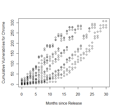
The figure shows the cumulative vulnerabilities reported for six releases of Chrome (Chrome 1.0 to 6.0) by the number of months since release. Different trends of different releases suggest that different discovery model should be applied for each release.

Figure 1: Google Chrome firework of vulnerability discovery trends

1.1 Contribution of this Paper

This paper presents an independent validation experiment on the goodness-of-fit of six existing VDMs against the three most popular browsers: Firefox, Google Chrome and Internet Explorer.

We also analyze the impact of vulnerability data sets based on different definitions of vulnerability to the VDM’s performance. Basically, the contribution of this paper is as follows.

• We introduce two qualitative metrics, namely goodness-to-fit entropy and goodness-of-fit quality, to assess the stability and quality of the goodness-of-fit of a VDM in a certain data set.

• We show that some model (AT) does not work at all. Reliability models do not seem to apply which is an empirical confirmation that security is essentially different than reliability. Among six analyzed models, AML seems to be superior in terms of goodness-of-fit quality.

• The definition of vulnerability does indeed impact the conclusion of a VDM study. If ones stick to a-vulnerability-as-an-NVD (e.g., NVD, NVD.Advice in our study) as the main source for counting, confirmed-by-vendors’ advisories NVD entries would yield more stable results than raw NVD.

• We found that long life evolving software may have more than one saturation periods when the number of discovered vulnerabilities slowly increase, but then continue increasing linearly. This probably is the effect of code inheritance i.e., a large amount of lines of code in the new code base is inherited from old ones.

The rest of the paper is organized as follows. In the subsequent section we present the related work (§2). Then we describe our research questions and how to find out the answers (§3). Next we briefly discuss existing VDMs and their formulae (§4). Then we present how we collect vulnerability data sets used for the validation purpose (§5). After that, we discuss the methodology to conduct the experiment, and a discussion about the result in our experiment (§6). Next, we discuss the impact of data sets to the goodness-of-fit of VDMs (§7). We then study the evolution of VDMs’ goodness-of-fit (§8), and the quality of VDMs (§9) in the software life cycles. After a discussion about potential threats (§10) to the validity of our work we conclude the paper (§11).

2 Related Work

Anderson [5] discussed the trade-off in security in open source and close source systems. On one side ‘to many eyes, all bugs are shallow’, but in the other side, ‘potential hackers have also had the opportunity to study the software closely to determine its vulnerabilities’. In this work, he proposed a VDM (a.k.a. Anderson Thermodynamic, AT) based on reliability growth models, in which the probability of a security failure at time $t$, when $n$ bugs have been removed, is in inverse ratio to $t$ for alpha testers. This probability is even lower for beta testers, $\lambda$ times more than alpha testers. However, he did not conduct any experiment to validate the proposed model.

In other work about vulnerability discovery between white hat (security researchers) and black hat (hackers), Rescorla [17] discussed many shortcomings of NVD, but his study heavily relies on it nonetheless. Rescorla proposed two mathematical models, called Linear model (a.k.a Rescorla Quadratic, RQ) and Exponential model (a.k.a Rescorla Exponential, RE). He has performed an experiment on four versions of different operation systems (i.e., Windows NT 4.0, Solaris 2.5.1, FreeBSD 4.0 and RedHat 7.0). All of the cases, the two models were able to fit the data with p-value ranged from $0.167$ to $0.589$. In fact, we could not find any significant difference between these models in term of goodness-of-fit by doing a Wilcoxson test on their reported result (p-value $>0.05$).

Alhazmi and Malaiya [2] proposed another VDM inspired by s-shape logistic model, called Alhazmi Malaiya Logistic (AML). The idea beyond is to divide the discovery process into three phases: learning phase, linear phase and saturation phase. In the first phase, people need some time to study the software, so less vulnerabilities are discovered. In the second phase, when people get deeper knowledge of the software, much more vulnerabilities are found. In the final phase, since the software is going out of date, not much people will use it. People lose interest in finding new vulnerabilities. So the cumulative vulnerabilities are stable. In this work, the authors validated their proposal against several versions of Windows (i.e., Win 95/98/NT4.0/2K) and Linux (i.e., RedHat Linux 6.1, 7.1). Their model fitted Win 95 very well (p-value = $0.999991$), and Win NT4.0 (p-value = $0.923$). For other versions, the p-value ranged from $0.054$ to $0.317$.

Alhazmi and Malaiya [3] compared their proposed model with Rescorla’s 2005 (RE, RQ) and Anderson’s 2002 (AT) on Windows 95/XP and Linux RedHat Linux 6.2, Fedora. The result shows that their logistic model has a better goodness-of-fit than others. For Windows 95 and Linux 6.2, as the vulnerabilities distribute along s-shape-like curves, only AML is able to fit it (p-value=1), whereas all other models fail to match the data (p-value $\leq 0.05$). For Windows XP, the story is different. RQ turns to be the best one with p-value$=0.97$, while AML poorly match the data (p-value=$0.147$).

Woo et al. [21] carried out an experiment on three browsers IE, Firefox and Mozilla. However, it is unclear which versions of these browsers were analyzed. We speculate that they did not distinguish between versions. This could have a significant impact to their final result as we show later in the paper. In their experiment, IE has not been fitted, Firefox was fairly fitted, and Mozilla was good fitted. From this result, we could not conclude any thing about the performance of AML.

In another experiment, Woo et al. [20] validated AML against two web servers: Apache and IIS. Also, they did not distinguish between versions of Apache and IIS. In this experiment, AML has demonstrated a very good performance on vulnerability data of these web servers (p-value $=1$).

3 Research Questions

The primary question is “does a model fit the observed data?". When a new VDM is proposed, the authors have done some experiment to validate the applicability of this VDM. Mostly, in their reports the proposed VDMs often have good goodness-of-fit measures. As time goes by, the goodness-of-fit may improve or deteriorate as more data become available (either in terms of data point for the same software or new software to be considered as an instance). This motivate our first research question:

RQ1

Are existing VDMs able to fit cumulative numbers of vulnerabilities of the popular browsers (i.e., IE, Firefox, and Chrome)?

To find the answer, we discovered another, major and almost foundational issue: “what is a vulnerability?". Most related work did not explicitly discuss this question. Normally, a vulnerability is a security report describing a particular problem of a particular application, for instance: a report in Mozilla Foundation Security Advisories (a.k.a an MFSA entry), or an NVD report of NIST (NVD entry). In the wisdom of many people, an NVD entry is a vulnerability, but there are many other definitions [18, 9, 8, 7, 6, 11]. This raises the second research question in our study.

RQ2

How do different definitions of vulnerability impact the VDMs’ goodness-of-fitness?

Figure 2 illustrates the vulnerability space of Firefox, in which different ’kinds’ of Firefox vulnerabilities are coexisted at different level of abstraction.

• Mozilla Bugzilla: contains very technical reports for vulnerabilities, but also other normal programming bugs. Bugzila entries, called bugs, are visualized as black circles in the figure.

• NVD: holds high level third-party security reports for several applications, including Firefox. Many NVD entries (gray ovals) mentioning Firefox maintain references to Bugzilla (black circles inside ovals).

• MFSA: are set of vendor’s high level security reports for Mozilla’s products. Each MFSA entry (rounded rectangle) always references to one or more bugs (black circles inside) responsible for this security flaw. MFSA also holds links to corresponding NVD entries (overlapped ovals).

Depend on the judgement of analysts, different numbers of vulnerabilities are observed and collected. Here, in Figure 2, if we define a vulnerability is an MFSA, or NVD, or Bugzilla, these numbers are respectively six, ten and fourteen. So which is the actual number of vulnerabilities? This is also the target of our third research question.

RQ3

Among vulnerability definitions, which is the most appropriate in which VDMs yield most stable result?

In the fourth research question, we address the fact that the fitness of a model might evolve over time. Then a model might only be good at some times, but be deteriorate later. Therefore, this research question focuses on the fitness of a VDM in the lifetime of software products.

RQ4

Among existing VDMs, which one is globally superior?

To work out these issues, we collected vulnerability-as-an-NVD data set for the three popular browsers. Then we fitted existing VDMs using observed data, and see how well they are (RQ3). Next, we collected other data sets with respect to other definitions, and fitted VDMs by these data sets (RQ3). We estimated the entropy of goodness-of-fit for each data set to know in which data set, VDMs may yield more stable result. This estimation is used to justify data sets (RQ3). And finally, we ranked VDMs based on their goodness-of-fit during the life time of software (RQ3).

This illustrates different abstract levels of vulnerability: developer level (Bugzilla) to user level (MFSA, Bugzilla). Bugzilla entry denotes technical programming issues (both security and non-security ones). Security bugzilla are ones reported in an MFSA, or referenced by an NVD.

Figure 2: The vulnerability space of Firefox.

4 Vulnerability Discovery Models

This section provides a quick glance about six VDMs. As denoted in [3], these VDMs are main features of the vulnerability discovery models. Here, only the formulae of these six models are discussed. The detail rationale of models as well as the meaning of each parameter can be found in the original work or in [3]. All these parameters are estimated using non-linear regression on observed data.

• Alhazmi-Malaiya Logistic (AML): proposed by Alhazmi & Malaiya [2], inspired by the s-shape curve. The rationale behind is the assumption that vulnerability discovery process is accounted into three phases. Learning phase: software has just been released, people need time to learn new software. Vulnerabilities are slowly detected. Linear phase: people get acquainted to the software, more vulnerabilities are rapidly discovered. Saturation phase: software becomes stable (or people move to new software), less vulnerabilities are discovered.

• Anderson Thermodynamic (AT): the application of this model to vulnerabilities is proposed by Anderson [5]. The author assumed that finding a vulnerability (or bug) after another one is much more harder as time goes by when the reliability of software increases. The term thermodynamic originates by the analogy from thermodynamics, in which $\gamma$ accounts for the lower failure rate during beta testing compared to higher rates during alpha testing.

• Linear model (LN): this is the simplest model, and well known by most people. Linear model is often used to express the trend line of data.

• Logistic Poisson (LP): is originated from the field of reliability engineering, also known as Musa-Okumoto model [15]. The idea of the model was that “the failure intensity would decrease exponentially with the expected number of failures experienced”[15]. In the formula, $\beta_{0}$ represents the total number of faults that would eventually be detected, $\beta_{1}$ is the per-fault hazard rate for the exponential model [12].

• Rescolar Exponential (RE): this model is a work of Rescorla [17], inspired by the Goel-Okumoto model[10] in software reliability engineering, in which the reliability is increasing. The number of vulnerabilities discovered in a single product is assumed to follow a Poisson process. Then, in the formulal, $N$ is the eventually total number of vulnerabilities, and $\lambda$ is the rate of discovery.

• Rescolar Quadratic (RQ): is also proposed in [17] while attempting to identify trends in the vulnerability discovery using statistical tests. The rationale behind is that the vulnerability finding rate varies linearly with time. The cumulative number of vulnerabilities is thus represented as a quadratic curve.

Table 1: Formal definitions of six VDMs in the study.

This table lists existing VDMs considered in the alphabetical order. The rationale of formulae and the meaning of each parameter should be found in original work of each model. All parameters are estimated based on non-linear regression on observed data.

Model	$\displaystyle Formula$
Alhazmi-Malaiya Logistic (AML)	$\displaystyle\Omega(t)=\frac{B}{BCe^{-ABt}+1}$
Anderson Thermodynamic (AT)	$\displaystyle\Omega(t)=\frac{K}{\gamma}\ln(t)+C$
Linear (LN)	$\displaystyle\Omega(t)=At+B$
Logistic Poisson (LP)	$\displaystyle\Omega(t)=\beta_{0}\ln(1+\beta_{1}t)$
Rescorla Exponential (RE)	$\displaystyle\Omega(t)=N(1-e^{-\lambda t})$
Rescorla Quadratic (RQ)	$\displaystyle\Omega(t)=\frac{At^{2}}{2}+Bt$

5 Data Collection

Vulnerability information for the three browsers IE, Firefox, and Chrome is available in multiple sources, from multi-vender source like National Vulnerability Database (NVD) to vendors’ advisories and bug trackers e.g., Mozilla Foundation Security Avisories (MFSA), Mozilla Bugzilla, or Chrome Issues Tracker. To evaluate the impact of vulnerability definitions to the goodness-of-fit of VDM, we collect different data sets with respective to different definitions.

Table 2: Data sets collected for major releases of IE, Firefox and Chrome.

Bullets ($\bullet$) indicate enabled data sets. Dashes (—), otherwise, mean there is no data sources available to collect the data sets.

	nvd	nvd.Bug	nvd.Advice	nvd.Nbug	advice.Nbug	Releases/Datasets
Chrome	$\bullet$	$\bullet$	—	$\bullet$	—	6/18(v1.0–v6.0)
Firefox	$\bullet$	$\bullet$	$\bullet$	$\bullet$	$\bullet$	6/30 (v1.0–v3.6)
IE	$\bullet$	—	$\bullet$	—	—	5/10 (v4.0–v8.0)
Total	17	12	11	12	6	17/58

• NVD(X): a vulnerability is an nvd entry that mentions version X (i.e., version X appears in the vulnerable configuration section of this nvd entry).

• NVD.Bug(X): a vulnerability is an nvd entry that mentions version X. And this nvd entry has one or more links in the references section to a bug report of the software vendor.

• NVD.Advice(X): a vulnerability is an nvd entry that mentions version X. And this nvd entry has one or more links in the references section to a security advisory report of the software vendor (the advisory report might not mention version X, but only some later version).

• NVD.Nbug(X): a vulnerability is a bug report of the vendor. This bug report also appears in the references section of an nvd entry that mentions version X.

• ADVICE.NBug(X): a vulnerability is a bug report of the software vendor. This bug report is also mentioned in an advisory report of the software vendor. This advisory report also has one or more links to an nvd entry that mentions version X. One exception is that many advisory reports of Firefox v1.0 have no link to NVD and we considered all bugs mentioned in these advisory reports as vulnerabilities for v1.0 even without nvd links.

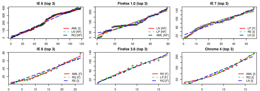
This figure illustrates feature goodness in Table 3. The circles indicate cumulative vulnerabilities at a certain time. The horizontal axis (X) is time-in-market measured by the number of months since officially released. The vertical axis (Y) is the cumulative vulnerabilities. Top 3 indicates the order of VDMs sorted by p-values. The label next to the VDM’s name in the legend shows the goodness-of-fit of this VDM.

Figure 3: VMDs’ goodness-of-fit on browsers in NVD data set.

In the NVD.NBug(X) and ADVICE.NBug(X), we do not know the releases that a bug might impact, we assume that a bug impact all configurations mentioned in the nvd referenced by this bug. However, not all bugs explicitly reference to nvd. In this case, we apply the bug-to-nvd linking scheme which includes following rules:

• if a bug is listed in the references of a nvd, this bug is linked to this nvd.

• if a bug and a nvd are clustered in an advisory report (e.g., mfsa), this bug is considered to be linked to this nvd.

We finally collected 58 data sets, and we used these data set to run the VDM experiment on 17 major releases of the three browsers. The detail of which data sets are available on which releases is reported in Table 2.

6 Validation of VDM

6.1 Validation Methodology

The steps of validating VDMs are quite straight forward. We first observe the data. Here, they are cumulative numbers of vulnerabilities monthly from the release date. Thus far all these models are mostly validated using vulnerability-is-an-NVD assumption, which corresponds to our NVD data set. Hence their data sets are collection of NVD entries published. To make our experiment comparable, we also use this definition of vulnerability, and run the goodness-of-fit experiment on the NVD data set. Besides, NVD is the only common data set among the three browsers (see Table 2).

Second, we fit VDMs into the all data points of the observed data using R[16] tool. Finally, expected values of each model are computed for the goodness-of-fit test. We employ chi-square ($\chi^{2}$) goodness-of-fit for this purpose. This test is based on $\chi^{2}$ statistics calculated as follows.

$$\chi^{2}=\sum_{i=1}^{n}\frac{(O_{i}-E_{i})^{2}}{E_{i}}$$ (1)

$O_{i}$ and $E_{i}$ orderly denote the oberseved values come from observation, and expected values generated by VDMs. The smaller $\chi^{2}$, the higher goodness a VDM gains. In practice, a VDM is acceptably fitted if the $\chi^{2}$ is less than a critical value, given a significant level ($\alpha$) and degrees of freedom. The p-value here represents the significance of the differences between observed values and expected values. If the p-value is small, differences are significant, not by chance. Thus, the smaller p-value, the stronger evidence a VDM does not fit the data. Hence, we interpret the goodness-of-fit based on the ranges of p-value as follows

• Not Fit: $\textit{p-value}\in[0\sim 0.05)$, the difference is significant, not by chance. This evidence is strong enough to reject the model.

• Good Fit: $\textit{p-value}\in[0.95\sim 1.0]$, the difference, in opposite to the previous, is significant small. It is a strong evidence to accept the model.

• Inconclusive Fit: $\textit{p-value}\in[0.05\sim 0.95)$, there is not enough evidence to neither reject nor accept the model.

6.2 Result and Discussion

We run the goodness-of-fit experiment for six VDMs on seventeen releases using NVD data set. The experiment generates 102 curves (and lines), so it is impossible to show them all. Figure 3, as for the illustrative purpose, only describes charts that highlight features in our result.

Among analyzed releases, many releases are old, which are shipped to users many years ago, and many releases have just been recently released. This diversification would provide us a good picture the behavior of VDMs in different period of application. Vulnerabilities of old releases are intuitively more stable than that of younger ones. Hence, a good VDM should be able to capture the vulnerability distribution of old releases.

To this extent, Figure 3 shows the fitted plots of VDMs in selected releases, i.e., IE6, IE7, IE8, Firefox v1.0–v3.6, Chrome 4, using NVD data set. We choose NVD data set to make our result comparable with others. We select these releases since they are more representative for two aforementioned groups of applications: old releases (i.e., IE6, Firefox v1.0, and IE7), and young releases (i.e., IE8, Firefox v3.6, and Chrome 4). In this figure, the cumulative numbers of vulnerabilities are illustrated as empty cycle, and fitted VDMs are visualized by lines with different patterns. We have six analyzed VDMs, but in this figure, we only show top three VDMs which have better results then others in terms of p-value.

The vulnerability distribution of IE6, and IE7 are still increasing in a nearly linear manner. This might be these following reasons. First, people are still interested in these two browsers since they are shipped with Windows XP which has a noticeable amount of users. Thus people keep searching vulnerabilities in these browsers. Second, there a lot amount of code base of IE6, 7 are inherited in later releases (i.e., IE8, IE9), then many vulnerabilities discovered later in IE8, IE9 are originated from retrospective releases (i.e., IE6, IE7).

This data distribution could explain the goodness-of-fit of VDMs which support linear modeling. Thus, in IE7, the LP model fitted the data very well, RQ and LN models might fit the data. Other models (not shown here) did not fit data well because their hypothesis shapes are not appropriate. Meanwhile, even though the increasing of IE6’s vulnerability seems to be linear, but the variance of numbers of vulnerabilities around the perfect linear model falsifies most VDMs, except AML since the observed data forms a stretched S-shape.

The chart of Firefox v1.0 shows a different phenomenon, called after-life vulnerabilities in which many vulnerabilities are discovered after a release is out of official support [14]. Vulnerabilities of Firefox v1.0 were discovered linearly in the first 20 months of life time, but then mostly constant in the next 20 months. However, this number is increasing later on until now. We speculate that when Firefox v1.0 was released, it attracted many attacks but later on people were losing interested in finding new vulnerabilities of this release. Then the number of vulnerabilities increased because a large portion of code in Firefox v1.0 is still alive in modern releases of Firefox [14]. And many vulnerabilities reported later are also applied to this very first release. This kind of distribution challenges all analyzed VDMs since none of analyzed VDMs taken this phenomenon into account, and hence they are all false for Firefox v1.0.

In the bottom parts of Figure 3, all the releases (IE8, Firefox v3.6, and Chrome 4) are still young. Thus the distribution of vulnerabilities for these releases are linear. So, many VDMs that address linear model could fit the data.

To have a overview picture about the performance of VDMs in NVD data set, Table 3 reports the goodness-of-fit for 102 curves of all releases. Here, instead of reporting a big table of numbers, Table 3 shows the interpretation of p-value of the $\chi^{2}$ tests. This presentation also helps to study at higher abstract level than the raw p-values. In this table, there are $47$ times VDMs can either well fit or inconclusively fit the data, and $55$ times they do not work. Roughly speaking, the chance of fit is about 50%. If we look at each VDM particularly, the AML model appears to be the best one as it obtains more positive results than others. In contract, the AT model seems to be the worst because it could only fit one release (IE v7.0). Meanwhile, other models are equivalent in number of times being rejected and accepted, except the LP model which is likely a bit better.

As a conclusion of this section, fitting VDMs into NVD data set give a hint that the assumption behind of the AML model is slightly appropriate to observed data. This idea apparently captures the way people discover vulnerability in practice. And in the first months of software’s lifetime, the vulnerabilities of software increases linearly. Hence, any models support linear modeling could be able to fit the observed data. However, depend on the shapes of the models, sometime a model is better than another ones. But we hardly say which one is better than the others, except, a more confidence conclusion about the performance of AT model, which very poor is almost cases. The assumption of AT model is completely not applicable for vulnerability detection.

However, since the goodness-of-fit of VDMs might change overtime, To have a better insight, in subsequent section, we will study the evolution of VDMs’ goodness-of-fit with respect to the software life time.

Table 3: The goodness-of-fit of VDMs using data set NVD.

The goodness of fit of a VDM is based on p-value in the $\chi^{2}$ test. $\textit{p-value}<0.05$: not fit (–), $\textit{p-value}\geq 0.95$: good fit (X), and inconclusive fit (?) otherwise.

	Firefox						Chrome						IE
Model	1.0	1.5	2.0	3.0	3.5	3.6	1.0	2.0	3.0	4.0	5.0	6.0	4.0	5.0	6.0	7.0	8.0
AML	–	–	?	?	?	?	X	?	?	?	?	?	X	?	?	–	X
AT	–	–	–	–	–	–	–	–	–	–	–	–	–	–	–	?	–
LN	–	–	X	–	X	?	–	–	–	?	–	–	–	–	–	?	?
LP	–	–	X	?	X	X	–	–	–	–	?	?	–	X	–	X	?
RE	–	–	X	?	X	X	–	–	–	–	?	?	–	X	–	?	?
RQ	–	–	–	?	?	X	–	–	?	?	?	?	–	–	–	–	X

7 The Impact of Data Sets

Figure 4 displays the notched box plots of browser releases and data sets to the observed cumulative vulnerabilities. The non-overlap notches between boxes indicate a statistically difference between their median. The distributions of vulnerabilities in data sets indeed reflect the way they are collected. If we take NVD data set as a base line, the NVD.Bug and NVD.Advice are subsets of NVD that only select nvd entries which have one or more confirmed links to a bug report or security advisory, respectively, by vendors. Thus, the numbers of vulnerabilities in NVD.Bug and NVD.Advice are less than NVD.

Meanwhile, NVD.Advice and NVD.Bug look quite similar. It is because many nvd entries which have links to vendors’ security advisories, also have links to vendors’ bug reports. So, these two data sets look the same. This is also confirmed by the statistical test. The Fligner-Killeen test on homogeneity of variances shows that NVD.Bug and NVD.Advice are pretty homogenous (p-value = $0.996$).

The NVD.Nbug and Advice.Nbug, respectively, count numbers of bugs in nvd entries and vendors’ security advisories. So, NVD.Nbug and Advice.Nbug are basically multipliers of NVD.Bug and NVD.Advice. Since a vendors’ security advisory entry, in the case of Firefox, often has more links to bug reports than a nvd entry does, the number of vulnerabilities of Advice.Nbug is larger than that of NVD.Nbug.

In general, the non-overlap notches (except NVD.Bug and NVD.Advice) show a statistically difference between the median among these five data sets. It gives a hint that different conclusions might be drawn from these data sets.

Figure 4: The box plots of the cumulative vulnerabilities of the data sets.

To better understand how data sets impact to the performance of VDMs, we compare the distribution of p-value generated by fitting each data set to all VDMs. To make the comparison more precise, we try to use at much data points as possible. However, since some data sets are not available for some browsers (see Table 2), we can only compare data sets in browsers that are supported by the data sets. In particular, we compare all five data sets in Firefox’s vulnerabilities because all these five data sets provide data for Firefox. For Chrome and Firefox, we can only compare NVD, NVD.Bug, NVD.Nbug. And for Firefox and IE, we can compare NVD and NVD.Advice. For IE, Firefox, and Chrome, NVD is the only data set support all these three browser, so we cannot make comparison.

The effect of different data sets to VDM is more clearly presented in Figure 5. This figure reports the p-values distribution of $\chi^{2}$-test of all VDMs across data sets. The leftmost box plot in this figure shows the difference among data sets while fitting Firefox’s vulnerabilities. Apparently, the p-value’s spectrum of NVD.Advice seems better than others: $50\%$ of the cases p-value is greater than $0.4$, whereas, $50\%$ of others is less than $0.2$. It means that the chances of getting a good fit by choosing NVD.Advice is greater than other models. This phenomenon is also appeared in the rightmost box plots for Firefox and IE. In the meanwhile, it seems there is not big difference among the medians of NVD, NVD.Bug and NVD.Nbug as demonstrated in the box plots of both Firefox and Firefox & Chrome. Though, NVD looks better than NVD.Bug and NVD.Nbug since its high quartile is greater than others’.

In summary, the analysis shows an evidence that counting vulnerabilities in different ways, which result in different vulnerability data sets, would impact to the overall quality of VDMs. And fitting the data of NVD.Advice, VDMs have more chances to obtain Good Fit. This means that existing VDMs can better model the trend of vulnerabilities that are both confirmed by NVD and vendors’ security advisories (NVD.Advice) than other data models.

Box plots showing the distribution of p-values of all VDMs across data sets. Left (a) shows the impact of data sets to the VDMs’ performance in Firefox. Middle (b) reports the impact of shared data sets between Firefox and Chrome, and Right (c) is the impact of shared data sets between IE and Firefox.

Figure 5: The impact of data sets to the quality of VDMs.

8 The Evolution of VDM’s Goodness-of-Fit in Data Sets

The observation done in the previous section (§7) provides an evidence that existing VDM can model the trend of vulnerabilities reported in NVD.Advice data set better than other data sets at the time when data sets are collected. For a better insight, this section aims to analyze whether this phenomenon is consistent for a long period or just happen by chance. The analysis result will also address the RQ3 about choosing the most appropriate data set that is more suitable for VDMs. The selection criteria are not only the data set that can be well modeled by VDMs (i.e., VDMs would obtain more Good Fit), but more important, the data set in which the performances of VDMs are more stable than in other data sets.

To this purpose we run the goodness-of-fit experiment during the life time of analyzed releases. For each release, we observe the evolution of VDMs’ goodness-of-fit with respect to the evolution of data set during the release’s life time. The life time of a software is the number of months since release time (MSR). The first MSR of a software is the end of the month after the released date. The second MSR is the end of month after the first MSR, and so on. For example, IE v4.0 is released in September, 1997. hence, the first MSR is on 31 October, 1997, and the first observation is on the sixth MSR, 31 March 1998. The observation begins at the sixth month when a release is officially shipped to users, and repeats monthly until the last day when data is collected. The cumulative numbers of vulnerabilities at observation points are fitted into all VDMs. The experiment generated $14,817$ curves in total.

There are three states in the model: Fit (F), Inconclusive(I) , and NotFit (NF). As more data available, a Fit model may remain Fit, or become Inconclusive, or NotFit. This evolution is represented by transitions. The labeled numbers on transitions denote transition’s names.

Figure 6: The goodness-of-fit transition model.

The box plots illustrate the distribution of VDMs’ goodness-of-fit entropy $E_{1}$ in different data sets. The calculation of entropy follows (2) with $\beta=1$.

Figure 7: Box plots of entropies ($\beta=1$).

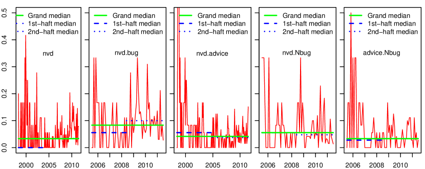
This figure shows the detail evolution of goodness-of-fit entropies of all data sets. The observation period for each type of data set depended on the the products’ lifetime supported by the data sets. The solid lines indicate the grand median of entropies in the whole period. The dash lines and dotted lines show the median of entropies for the first-half and second-half period. The performance of VDMs are more stable if the median of the second-half is less than or equal the median of the first-half.

Figure 8: The evolution of goodness-of-fit entropies of all data sets.

Let us consider one VDM. When fitting data to this VDM, we can get either Good Fit, or Inconclusive, or Not Fit. Suppose that at the observation time $t$ and $t+1$, the goodness-of-fits are $GoF_{t}$, and $GoF_{t+1}$, respectively. If $GoF_{t}$ equals $GoF_{t+1}$, we say that the VDM is stable during period $(t..t+1)$, otherwise the VDM is unstable. We introduce a measurement for the stable of VDMs, called goodness-of-fit entropy, by counting the number of times that the goodness-of-fit of a VDM changes.

To formally define the goodness-of-fit entropy, we use the goodness-of-fit transition model as depicted in Figure 6. The model consists of three states: Fit (F), Inconclusive (I), and Not Fit (NF). The VDMs’ goodness-of-fits are initially classified into one of these states in the 6th MSR. The goodness-of-fit states can be subsequently evolved to other states according to the transitions. The model has total nine transitions labeled from 1 to 9, denoted as #$i$, falling into one of three categories, unchanged, small jump, and big jump. The unchanged transitions (#$1$, #$2$, and #$3$) mean the states are unchanged, in order words, there is no entropy. The small jump transitions (#$4$–#$7$) denote a smaller change (compared to big jump) of p-value from Good Fit ($\geq 0.95$) to Inconclusive ($[0.05..0.95))$, or from Inconclusive to Not Fit ($<0.05$), and vice versa. In the meanwhile, big jump transitions (#$8$,#$9$) show a big change from Good Fit to Not Fit and versa.

The goodness-of-fit entropy at observation time $t$ is estimated by counting the number of transitions when moving from time $t-1$ to time $t$. Since the the levels of instability of transitions are not equal, the contribution of different kinds of transition into the overall entropy might be different. Since unchanged transitions do not contribute to the entropy, we define $\beta$ as the factor that big jump is $\beta$ times as chaos as small jump. The calculation of goodness-of-fit entropy follows this equation:

$$E_{\beta}(t)=\frac{\displaystyle|smalljump|_{t}+\beta\cdot|bigjump|_{t}}{\displaystyle|unchanged|_{t}+|smalljump|_{t}+\beta\cdot|bigjump|_{t}}$$ (2)

where $|XXjump|_{t}$ is the numbers of $XXjump$ transitions when moving from time $t-1$ to time $t$.

The goodness-of-fit entropy measured in (2) ranges from 0 to 1. Entropy equals 0 when $|smalljumps+bigjump|=0$. It denotes a local stability of goodness-of-fit when moving from time $t-1$ to time $t$. On the contrary, entropy equals 1 when $|unchanged|=0$, which is a complete chaos.

conclusion: These small medians show an evidence that VDMs’s goodness-of-fits are somehow stable within these data sets. In detail, the overlapped notches among NVD, NVD.Advice, NVD.Nbug and ADVICE.Nbug give a hint that the stability of VDMs in these data sets is not much different. Meanwhile, the median of NVD.bug is significant greater than others’.

The box plots in Figure 7 report the distribution of the evolution of goodness-of-fit entropies. Generally, about $75\%$ of the cases of most data sets, the entropy is less than $0.1$. Moreover, the overlapped notches among NVD, NVD.Advice, NVD.Nbug and ADVICE.Nbug give a hint that the medians of entropy of these four data set are not statistically different. Meanwhile, the median of NVD.bug is significant greater than others’. This observation is confirmed by the Kruskal-Wallis rank sum test on the variance of entropies. The null hypothesis is “there is no difference between the median of entropies among data sets". The Kruskal-Wallis test four data sets NVD, NVD.Advice, NVD.Nbug and ADVICE.Nbug yields p-value = $0.271$, which means we do not have enough evidence to conclude about the difference their medians. And the Kruskal-Wallis test for all five data sets yields p-value = $0.0040$, which confirms the significant different of NVD.Advice and other data sets.

To understand how entropies evolve, we divide the observation period of each data sets into two parts, namely first-half and second half, then we calculate the median for two parts. A stable evolution would result that the entropy median of the first-half is greater (or equal) the entropy median of the second-half. It is because the decreasing of entropy median means the VDMs become more stable as more data are available in the data set.

Figure 8 shows the evolution of goodness-of-fit entropy for each data set. The solid lines indicate the grand medians for the whole observation periods. The dash lines denotes the medians of the first half periods and dotted lines illustrate the medians of the second half periods. Notice that the grand medians of the plot are exactly the medians of data sets illustrated in Figure 7. This is obvious since the Figure 7 is the summary view of Figure 8.

Look at the trends of evolution, the entropy variation of NVD.Advice seems to be lesser than other data sets. Moreover the second half median of NVD.Advice is less than the first haft median. So, NVD.Advice seems to be a good candidate data set. The NVD.Nbug also has the median of the second half less than the median of the second half, but the entropy variation of NVD.Nbug in the second half looks bigger than that of NVD.Advice. In the opposite direction, NVD.Bug is very bad. The plot of entropy is very dynamic, especially in the second half. The entropy median increases in the second half period, which might imply a more instability performance of VDMs.

To ensure that NVD.Bug is a worst one, we additional employ one-side Mann-Whiney U test to perform pairwise tests between the entropies of NVD.Bug and others’ with the alternative hypothesis “the entropy distribution of NVD.Bug is stochastic larger than others". Notice that, since multiple comparisons are employed, Bonferroni correction is applied with the number of tests $n=4$, so the significance level $\alpha^{\prime}=\nicefrac{{0.05}}{{4}}=0.0125$. The result of these tests shows that the entropy variation of NVD.Bug is larger than NVD (p-value $=1.82\cdot 10^{-4}$), NVD.Advice (p-value $=1.3\cdot 10^{-3}$), and ADVICE.Nbug (p-value $=0.004$). For the comparison test between NVD.Bug and NVD.Nbug, the p-value $=0.06>\alpha^{\prime}$. Even though it is not enough evidence to conclude, but it is very near to the point that the entropy variation of NVD.bug is larger than that of NVD.Nbug.

In summary, all five analyzed data sets achieve a good stability for VDMs’ goodness-of-fit performance in overall. The entropy of VDMs’ performance is less than 0.2% (0 - for perfect stability, and 1 - for completely dynamic) for all data sets. Among the data sets, NVD.bug is the worst it is significantly more unstable than other data sets, and more importantly, NVD.bug tends to be more unstable when more data are available (i.e., entropy of the second-half period is greater than that of the first-half period). In the other side, NVD.Advice is slightly better than others. Even though there is no significant difference among medians, NVD.Advice is apparently the appropriate data sets for VDMs because VDMs’ goodness-of-fits in these data sets are more stable when more data is available.

9 The Temporal Quality of VDM

This section addresses the research question RQ3. To know which VDM is globally better than other, we analyze the performance of VDMs in the life time of analyzed releases. We introduce another measurement for the performance of a VDM, namely goodness-of-fit quality $Q$ (or quality for short).

The quality of a VDM depends on how well it can fit the vulnerability data of analyzed releases. Thus this quality measurement can vary over time since the vulnerability data evolve over time as we can see in the previous section (§8). The VDM’s quality at time $t$ is measured by the ratio between the number of Good Fits (p-value of $\chi^{2}$ goodness-of-fit $\geq 0.95$) by the total number of fits at time $t$. Besides, since we could not conclude about an Inconclusive Fit when its p-value ranged from $0.05$ to $0.95$, an Inconclusive Fit also contributes to the overall quality, but may be not as good as a Good Fit. Thus, we use an extra factor $\omega$ to denote that a Good Fit is $\omega$ times as good as an Inconclusive Fit. The formula is defined as follows.

$$Q_{\omega}(t)=\frac{|Fit|_{t}+\nicefrac{{1}}{{\omega}}\cdot|Inconclusive|_{t}}{|Fit|_{t}+|Inconclusive|_{t}+|NotFit|_{t}}$$ (3)

where $|X|_{t}$ is the number of times a VDM obtains goodness-of-fit $X$ at time $t$ ($X$ is Fit, Inconclusive or Not Fit). $Q_{\omega}(t)$ is distributed from 0 to 1. $Q_{\omega}(t)=0$ indicates a VDM does not fit any data; and, $Q_{\omega}(t)=1$ shows that a VDM can fit all data very well.

Figure 9 shows the notched box plots of global goodness-of-fit quality of VDMs. Top are plots of VDMs’ quality no mater what the data sets. Bottom are the similar plots but restricted to NVD.Advice data set only. To additionally evaluate how the difference between a Good Fit and an Inconclusive ($\omega$ factor) impacts the the final quality, left plots show the VDMs’ quality where a Good Fit is as good as an Inconclusive ($\omega=1$); and right plots shows the VDMs’ quality where a Good Fit is twice as good as an Inconclusive ($\omega=2$).

If we ignore the data sets (top plots), Roughly 75% of the case AML model has a better quality than other models. Meanwhile, the quality of AT model is the worst. This is true regardless the value of $\omega$. For other models, the plots shows that there is not much different among LN, LP and RE models. The RQ is slightly worse than others since the first quartile of the distribution is much lower than others’.

Previous section has showed that NVD.Advice is slightly better than other data sets. So, in the bottom plots, we analyze the quality of VDMs in NVD.Advice. Here, we observe the same phenomenon for both AML and AT models. For other models, LP and RE look like the same; but LN and RQ models are slightly better.

Top charts show the quality of VDMs in all data sets. Meanwhile, bottom charts illustrate the quality of VDMs in NVD.Advice data sets. In left charts, a Good Fit is as good as an Inconclusive Fit ($\omega=1$). And in the right charts, a Good Fit is twice as good as an Inconclusive Fit ($\omega=2$).

Figure 9: The VDMs’ goodness-of-fit quality.

This result is quite compliant with the previous analysis in NVD data set at the time data collected (see §6). This would allow us to make stronger conclusions about the performance of analyzed VDM.

First, AT model is absolutely not a right model for vulnerability discovery process. It means that the rationale behind the AT model is not applicable for vulnerability detection. Besides, the two model LP and RE also do not obtain a good quality comparing to other models, especially the AML model. If we consider an Inconclusive Fit is half as good as a Good Fit, and we use the NVD.Advice, the qualities of these two models, LP and RE, are even lower than other models. Thus, AT, LP, RE model are indeed not good options for vulnerability detection. These three models share a common point that is they are all based on reliability models using to express the discovery process of normal bugs. The core difference between reliability models and VDM is the motivation of detectors. In the former, detectors are software engineers (testers, quality control), so they only invest on finding bugs so that the reliability of an application reaches to a certain threshold. In the later, whereas, detectors are the whole community who are interested in the application. The motivation of finding a vulnerability therefore much bigger than finding a normal bug, and also last for longer time (depend on the number of users of an application). Existing reliability-based VDMs which do not capture this phenomenon could not obtain good performance.

Notably, the three model AT, RE, LP are both based on reliability models, but the RE and LP could obtain better performance that the AT model. This is true because of the shapes of each model. The shape of AT model does not express very well the first period of vulnerability discovery when vulnerabilities are found in an (approximately) linear manner. The RE and LP, whereas, can do this better. Hence, AT model fails most of the cases, and RE and LP models still obtain good results when the evolution of vulnerability is linear.

Second, AML model is better than other model since its assumptions match better the actual behavior of community in finding vulnerability of a software.

10 Threats to Validity

Bias in data collection.

This work employs the same technique discussed in [13] to parse HTML pages of MFSA, and process the XML data of NVD and Bugzilla. Even though the collector tool has been checked for multiple times, it might contain bugs affecting to data collection.

Bias in bug-to-nvd linking scheme.

While collecting data for ADVICE.Nbug, we apply some rules to link a bug to an nvd based on their locations in the MFSA report. Nevertheless, this might be incorrect. We manually checked some links for the relevant connection between bug reports and NVD entries. They were found to be consistent. However, again, it might not be always true.

Overestimation of number of bugs in each version.

We do not know exactly which versions that a bug affects. Consequently, we assume that a bug affects all versions mentioned in the linked nvd. This might overestimate the number of vulnerabilities in each version. To mitigate the problem, we calculate the latest release that a bug might impact, and filter all vulnerable releases after this latest. This calculation is done using the bug fixes mining technique discussed in [19].

Error in curve fitting.

We estimate the goodness-of-fit of VDMs by using the Nonlinear Least-Square technique implemented in R (nls() function). This might not produce the most optimal solution. That essentially impacts the validity of this work. To mitigate this issue, we additionally employ a commercial tool i.e., CurveExpert Pro to cross check the goodness-of-fit.

Bias in statistic tests.

Our conclusions are based on statistics tests. These tests have their own assumptions. Choosing tests whose assumptions are violated might end up with wrong conclusions. To reduce the risk we carefully analyzed the assumptions of the tests, for instance, we did not apply any tests with normality assumption since the distribution of vulnerabilities is not normal.

11 Conclusion

In this work we addressed a fundamental question in vulnerability discovery modeling “do existing VDMs work?". We have conducted an experiment in which we fitted six existing VDMs (i.e., AML, AT, LN, LP, RE and RQ) to fifty eight data sets of seventeen releases of three popular web browsers IE, Firefox and Chrome.

This experiment confirmed that the assumption behind of the AML model, which vulnerability discovery process follow three phases: learning, linear, and saturation, is more appropriate to observed data. This idea apparently captures the way people discover vulnerability in practice. However, in the case of Firefox, since a large portion of the old code based is inherited in modern releases [14], therefore many vulnerabilities of the very first releases (e.g., v1.0, v1.5) continue to increase after a period of saturation even though these releases are retired (out of support). It explains for the not fit results of all of VDMs in these releases since none of them is able to capture this phenomenon.

In the opposite side, AT model performance is very poor. We can conclude that the assumption of this model is completely not applicable for vulnerability detection. We speculate that people are more passionate in finding vulnerabilities rather than normal bugs. Meanwhile software testers only focus on finding bugs until the reliability level of the software reaches to a certain threshold. This also explain for that AML is slightly better than other Reliability-based models (i.e., RE, LP). The performance of LN, RE, LP are approximate because vulnerabilities of many of analyzed releases are more or less in the linear phase.

The investigation on the evolution of goodness-of-fit entropy and quality reports a notable impact of the data set selection to the quality of a VDM, even though there is no statistically difference of the goodness-of-fit entropy among data sets. The NVD.Advice data set emerges as the best one in terms of entropy (even though slightly), and quality.

However, this experiment is only based on one kind of application. This might limit the final result. Therefore, as part of future work, more similar experiments on other kinds of applications, e.g., operating systems, web server applications, should be conducted in order to have solid conclusions.

References

- Alhazmi and Malaiya [2005a] O. Alhazmi and Y. Malaiya. Quantitative vulnerability assessment of systems software. In Proc. of RAMS’05, pages 615–620, 2005a.
- Alhazmi and Malaiya [2005b] O. Alhazmi and Y. Malaiya. Modeling the vulnerability discovery process. In Proc. of the 16th IEEE Int. Symp. on Software Reliab. Eng. (ISSRE’05), pages 129–138, 2005b.
- Alhazmi and Malaiya [2008] O. Alhazmi and Y. Malaiya. Application of vulnerability discovery models to major operating systems. IEEE Trans. on Reliab., 57(1):14–22, 2008.
- Alhazmi et al. [2005] O. Alhazmi, Y. Malaiya, and I. Ray. Security vulnerabilities in software systems: A quantitative perspective. Data and App. Sec. XIX, 3654:281–294, 2005.
- Anderson [2002] R. Anderson. Security in open versus closed systems - the dance of Boltzmann, Coase and Moore. In Proc. of Open Source Soft.: Economics, Law and Policy, 2002.
- Arbaugh et al. [2000] W. A. Arbaugh, W. L. Fithen, and J. McHugh. Windows of vulnerability: A case study analysis. IEEE Comp., 33(12):52–59, 2000.
- Avizienis et al. [2004] A. Avizienis, J.-C. Laprie, B. Randell, and C. Landwehr. Basic concepts and taxonomy of dependable and secure computing. IEEE Transactions On Dependable And Secure Computing, 1(1):11–33, 2004.
- Computer Science and Telecommunications Board [2001] Computer Science and Telecommunications Board. Computers at risk: Safe computing in the information age. National Academy Press, 2001.
- Dowd et al. [2007] M. Dowd, J. McDonald, and J. Schuh. The art of software security assessment. Addision-Wesley publications, 2007.
- Goel and Okumoto [1979] A. L. Goel and K. Okumoto. Time-dependent error-detection rate model for software reliability and other performance measures. Transactions on Reliability, 28(3):206–211, August 1979.
- Krsul [1998] I. V. Krsul. Software Vulnerability Analysis. PhD thesis, Purdue University, 1998.
- Malaiya et al. [1993] Y. K. Malaiya, A. von Mayrhauser, and P. K. Srimani. An examination of fault exposure ratio. IEEE Trans. Softw. Eng., 19:1087–1094, November 1993. ISSN 0098-5589.
- Massacci and Nguyen [2010] F. Massacci and V. H. Nguyen. Which is the right source for vulnerabilities studies? an empirical analysis on mozilla firefox. In Proc. of MetriSec’10, 2010.
- Massacci et al. [2011] F. Massacci, S. Neuhaus, and V. H. Nguyen. After-life vulnerabilities: A study on firefox evolution, its vulnerabilities and fixes. In Proc. of ESSoS’11, February 9-10 2011.
- Musa and Okumoto [1984] J. D. Musa and K. Okumoto. A logarithmic poisson execution time model for software reliability measurement. In Proceedings of the 7th international conference on Software engineering, ICSE ’84, pages 230–238, Piscataway, NJ, USA, 1984. IEEE Press. ISBN 0-8186-0528-6.
- R Development Core Team [2011] R Development Core Team. R: A Language and Environment for Statistical Computing. R Foundation for Statistical Computing, Vienna, Austria, 2011. URL http://www.R-project.org. ISBN 3-900051-07-0.
- Rescorla [2005] E. Rescorla. Is finding security holes a good idea? IEEE Sec. and Privacy, 3(1):14–19, 2005.
- Schneider [1991] F. B. Schneider. Trust in cyberspace. National Academy Press, art. CSTB study edited by Schneider, 1991.
- Sliwerski et al. [2005] J. Sliwerski, T. Zimmermann, and A. Zeller. When do changes induce fixes? In Proc. of the 2nd Int. Working Conf. on Mining Soft. Repo. MSR(’05), pages 24–28, May 2005.
- Woo et al. [2006a] S.-W. Woo, O. H. Alhazmi, and Y. K. Malaiya. Assessing vulnerabilities in apachee and iis http servers. In Proc. of the 2nd IEEE International Symposium on Dependable Autonomic and Secure Computing, 2006a.
- Woo et al. [2006b] S.-W. Woo, O. H. Alhazmi, and Y. K. Malaiya. An analysis of the vulnerability discovery process in web browsers. In Proc. of 10th IASTED SEA’06, November 13–15 2006b.
- Woo et al. [2011] S.-W. Woo, H. Joh, O. H. Alhazmi, and Y. K. Malaiya. Modeling vulnerability discovery process in apache and iis http servers. Computers & Security, 30(1):50 – 62, 2011.