A Multi-Agent Prediction Market based on Partially Observable Stochastic Game

We present a novel, game theoretic representation of a multi-agent prediction market using a partially observable stochastic game with information (POSGI). We then describe a correlated equilibrium (CE)-based solution strategy for this game which enables each agent to dynamically calculate the prices at which it should trade a security in the prediction market. We have extended our results to risk averse traders and shown that a Pareto optimal correlated equilibrium strategy can be used to incentively truthful revelations from risk averse agents. Simulation results comparing our CE strategy with five other strategies commonly used in similar markets, with both risk neutral and risk averse agents, show that the CE strategy improves price predictions and provides higher utilities to the agents as compared to other existing strategies.

1 Introduction

Forecasting the outcome of events that will happen in the future is a frequently indulged and important task for humans. It is encountered in various domains such as forecasting the outcome of geo-political events, betting on the outcome of sports events, forecasting the prices of financial instruments such as stocks, and casual predictions of entertainment events. Despite the ubiquity of such forecasts, predicting the outcome of future events is a challenging task for humans or even computers - it requires extremely complex calculations involving a reasonable amount of domain knowledge, significant amounts of information processing and accurate reasoning. Recently, a market-based paradigm called prediction markets has shown ample success to solve this problem by using the aggregated ‘wisdom of the crowds’ to predict the outcome of future events. This is evidenced from the successful predictions of actual events done by prediction markets run by the Iowa Electronic Marketplace(IDEM), Tradesports, Hollywood Stock Exchange, the Gates-Hillman market [26], and by companies such as Hewlett Packard [29], Google [7] and Yahoo’s Yootles [34]. A prediction market for a real-life event (e.g., “Will Obama win the 2008 Democratic Presidential nomination?”) is run for several days before the event happens. The event has a binary outcome (yes/no or $1/0$). On each day, humans, called traders, that are interested in the outcome of the event express their belief on the possible outcome of the event using the available information related to the event. The information available to the different traders is asymmetric, meaning that different traders can possess bits and pieces of the whole information related to the event. The belief values of the traders about the outcome of the event are expressed as probabilities. A special entity called the market maker aggregates the probabilities from all the traders into a single probability value that represents the possible outcome of the event. The main idea behind the prediction market paradigm is that the collective, aggregated opinions of humans on a future event represents the probability of occurrence of the event more accurately than corresponding surveys and opinion polls. Despite their overwhelming success, many aspects of prediction markets such as a formal representation of the market model, the strategic behavior of the market’s participants and the impact of information from external sources on their decision making have not been analyzed extensively for a better understanding. We attempt to address this deficit in this paper by developing a game theoretic representation of the traders’ interaction and determining their strategic behavior using the equilibrium outcome of the game. We have developed a correlated equilibrium (CE)-based solution strategy for a partially observable stochastic game representation of the prediction market. We have also empirically compared our CE strategy with five other strategies commonly used in similar markets, with both risk neutral and risk averse agents, and showed that the CE strategy improves price predictions and provides higher utilities to the agents as compared to other existing strategies.

2 Related Work

Prediction markets were started in 1988 at the Iowa Electronic Marketplace [19] to investigate whether betting on the outcome of gee-political events (e.g. outcome of presidential elections, possible outcome of international political or military crises, etc.) using real money could elicit more accurate information about the event’s outcome than regular polls. Following the success of prediction markets in eliciting information about events’ outcomes, several other prediction markets have been started that trade on events using either real or virtual money. Prediction markets have been used in various scenarios such as predicting the outcome of gee-political events such as U.S. presidential elections, determining the outcome of sporting events, predicting the box office performance of Hollywood movies, etc. Companies such as Google, Microsoft, Yahoo and Best Buy have all used prediction markets internally to tap the collective intelligence of people within their organizations. The seminal work on prediction market analysis [13, 32, 33] has shown that the mean belief values of individual traders about the outcome of a future event corresponds to the event’s market price. Since then researchers have studied prediction markets from different perspectives. Some researchers have studied traders’ behavior by modeling their interactions within a game theoretic framework. For example, in [3, 11] the authors have used a Shapley-Shubik game that involves behavioral assumptions on the agents such as myopic behavior and truthful revelations and theoretically analyzed the aggregation function and convergence in prediction markets. Chen et. al. [4] characterized the uncertainty of market participants’ private information by incorporating aggregate uncertainty in their market model. However, both these models consider traders that are risk-neutral, myopic and truthful. Subsequently, in [6] the authors have relaxed some of these assumptions within a Bayesian game setting and investigated the conditions under which the players reveal their beliefs truthfully. Dimitrov and Sami [9] have also studied the effect of non-myopic revelations by trading agents in a prediction market and concluded that myopic strategies are almost never optimal in the market with the non-myopic traders and there is a need for discounting. Other researchers have focused on designing rules that a market maker can use to combine the opinions (beliefs) from different traders. Hanson [15] developed a market scoring rule that is used to reward traders for making and improving a prediction about the outcome of an event. He further showed how any proper scoring rule can serve as an automated market maker. Das [8] studied the effect of specialized agents called market-makers which behave as intermediaries to absorb price shocks in the market. Das empirically studied different market-making strategies and concludes that a heuristic strategy that adds a random value to zero-profit market-makers improves the profits in the markets.

The main contribution of our paper, while building on these previous directions, is to use a partially observable stochastic game (POSG) [14] that can be used by each agent to reason about its actions. Within this POSG model, we calculate the correlated equilibrium strategy for each agent using the aggregated price from the market maker as a recommendation signal. We have also considered the risk preferences of trading agents in prediction markets and shown that a Pareto optimal correlated equilibrium solution can incentively truthful revelation from risk averse agents. We have compared the POSG/correlated equilibrium based pricing strategy with five different pricing strategies used in similar markets with pricing data obtained from real prediction prediction market events. Our results show that the agents using the correlated equilibrium strategy profile are able to predict prices that are closer to the actual prices that occurred in real markets and these traders also obtain $35-127\%$ higher profits.

3 Preliminaries

Prediction Market. Our prediction market consists of $N$ traders, with each trader being represented by a software trading agent that performs actions on behalf of the human trader. The market also has a set of future events whose outcome has not yet been determined. The outcome of each event is considered as a binary variable with the outcome being $1$ if the event happens and the outcome being $0$ if it does not. Each outcome has a security associated with it. A security is a contract that yields payments based on the outcome of an uncertain future event. Securities can be purchased or sold by trading agents at any time during the lifetime of the security’s event. A single event can have multiple securities associated with it. Trading agents can purchase or sell one or more of the securities for each event at a time. A security expires when the event $e$ associated with it happens at the end of the event’s duration. At this point the outcome of the event has just been determined and all trading agents are notified of the event’s outcome. The trading agents that had purchased the security during the lifetime of the event then get paid $\$1$ if the event happens with an outcome of $1$, or, they do not get paid anything and lose the money they had spent on buying the security if the event happens with an outcome of $0$. On each day, a trading agent makes a decision of whether to buy some securities related to ongoing events in the market, or whether to sell or hold some securities it has already purchased.

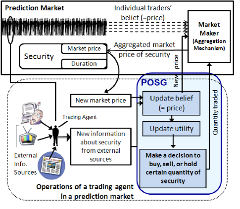
Figure 1: Essential operations performed by a trading agent in a prediction market and the portion of the prediction market where the POSG representation is applied.

Market Maker. Trading in a prediction market is similar to the continuous double auction (CDA) protocol. However, using the CDA directly as the trading protocol for a prediction market leads to some problems such as the thin market problem (traders not finding a trading partner immediately) and traders potentially losing profit because of revealing their willingness to trade beforehand to other traders. To address these problems, prediction markets use a trading intermediary called the market maker. The market maker aggregates the buying and selling prices of a security reported in the trades from the trading agents (they can be identical) and ‘posts’ these prices in the market. Trading agents interact with the market maker to buy and sell securities, so that they do not have to wait for another trading agent to arrive before they can trade. A market maker uses a market scoring rule (MSR) to calculate the aggregated price of a security. Recently, there has been considerable interest in analyzing the MSRs [5, 15, 27] and an MSR called the logarithmic MSR (LMSR) has been shown to guarantee truthful revelation of beliefs by the trading agents [15]. LMSR allows a security’s price, and payoffs to agents buying/selling the security, to be expressed in terms of its purchased or outstanding quantity. Therefore, the ‘state’ of the securities in the market can be captured only using their purchased quantities. The market-maker in our prediction market uses LMSR to update the market price and to calculate the payoffs to trading agents. We briefly describe the basic mechanism under LMSR. Let $\Xi$ be the set of securities in a prediction market and $\overline{q}=(q_{1},q_{2}...q_{|\Xi|})$ denote the vector specifying the number of units of each security held by the different trading agents at time $t$. The LMSR first calculates a cost function to reflect the total money wagered in the prediction market by the trading agents as: $C(\overline{q})=b\cdot ln(\sum_{j=1}^{\mid\Xi\mid}e^{q_{j}/b})$. It then calculates the aggregated market price $\pi$ for the security $\xi\in\Xi$ as: $\pi_{\xi}=e^{(q_{\xi}/b)}/\sum_{j=1}^{\mid\Xi\mid}(e^{(q_{j}/b)})$ [5] . Trading agents inform the quantity of a security they wish to buy or sell to the market maker. If a trading agent purchases $\delta$ units of a security, the market maker determines the payment the agent has to make as $C(\overline{q}+\delta)-C(\overline{q})$. Correspondingly, if the agent sells $\delta$ quantity of the security, it receives a payoff of $C(\overline{q})-C(\overline{q}-\delta)$ from the market maker. Figure 1 shows the operations performed by a trader (trading agent) in a prediction market and the portions of the prediction market that are affected by the POSG representation described in the next section.

4 Partially Observable Stochastic Games for Trading Agent Interaction

For simplicity of explanation, we consider a prediction market where a single security is being traded over a certain duration. This duration is divided into trading periods, with each trading period corresponding to a day in a real prediction market. The ‘state’ of the market is expressed as the quantity of the purchased units of the security in the market. At the end of each trading period, each trading agent receives information about the state of the market from the market maker. With this prior information, the task of a trading agent is to determine a suitable quantity to trade for the next trading period, so that its utility is maximized. In this scenario, the environment of the agent is partially observable because other agents’ actions and payoffs are not known directly, but available through their aggregated beliefs. Agents interact with each other in stages (trading periods), and in each stage the state of the market is determined stochastically based on the actions of the agents and the previous state. This scenario directly corresponds to the setting of a partially observable stochastic game [12, 14]. A POSG model offers several attractive features such as structured behavior by the agents by using best response strategies, stability of the outcome based on equilibrium concepts, lookahead capability of the agent to plan their actions based on future expected outcomes, ability to represent the temporal characteristics of the interactions between the agents, and, enabling all computations locally on the agents so that the system is robust and scalable.

Previous research has shown that information related parameters in a prediction market such as information availability, information reliability, information penetration, etc., have a considerable effect on the belief (price) estimation by trading agents. Based on these findings, we posit that a component to model the impact of information related to an event should be added to the POSG framework. With this feature in mind, we propose an interaction model called a partially observable stochastic game with information (POSGI) for capturing the strategic decision making by trading agents. A POSGI is defined as:
$\Gamma=(N,S,(A_{i})_{i\in N},(R_{i})_{i\in N},T,(O_{i})_{i\in N},\Omega,({\cal I}_{i})_{i\in N})$, where $N$ is a finite set of agents, $S$ is a finite, non-empty set of states - each state corresponding to certain quantity of the security being held (purchased) by the trading agents. $A_{i}$ is a finite non-empty action space of agent $i$ s.t. $\overline{a_{k}}=(a_{1,k},...,a_{|N|,k})$ is the joint action of the agents and $a_{i,k}$ is the action that agent $i$ takes in state $k$. In terms of the prediction market, a trading agent’s action corresponds to certain quantity of security it buys or sells, while the joint action corresponds to changing the purchased quantity for a security and taking the market to a new state. $R_{i,k}$ is the reward or payoff for agent $i$ in state $k$ which is calculated using the LMSR market maker. $T:T(s,\overline{a},s^{\prime})=P(s^{\prime}|s,\overline{a})$ is the transition probability of moving from state $s$ to state $s^{\prime}$ after joint action $\overline{a}$ has been performed by the agents. $O_{i}$ is a finite non-empty set of observations for agent $i$ that consists of the market price and the information signal, and $o_{i,k}\in O_{i}$ is the observation agent $i$ receives in state $k$. $\Omega:\Omega(s_{k},I_{i,k},o_{i,k})=P(o_{i,k}|s_{k},I_{i,k})$ is the observation probability for agent $i$ of receiving observation $o_{i,k}$ in state $s_{k}$ when the information signal is $I_{i,k}$. Finally, ${\cal I}_{i}$ is the information set received by agent $i$ for an event ${\cal I}_{i}=\bigcup_{k}I_{i,k}$ where $I_{i,k}\in\{-1,0,+1\}$ is the information received by agent $i$ in state $k$. The complete information arriving to the market ${\cal I}=\bigcup_{i\in N}{\cal I}_{i}$ is temporally distributed over the duration of the event, and, following the information arrival patterns observed in stock markets [23], we assume that new information arrives following a Poisson distribution. Information that improves the probability of the positive outcome of the event is considered positive($I_{i,k}=+1$) and vice-versa, while information that does not affect the probability is considered to have no effect ($I_{i,k}=0$). For example, for a security related to the event “Obama wins 2008 presidential elections”, information about Oprah Winfrey endorsing Obama would be considered high impact positive information and information about Obama losing the New Hampshire Primary would be considered negative information.

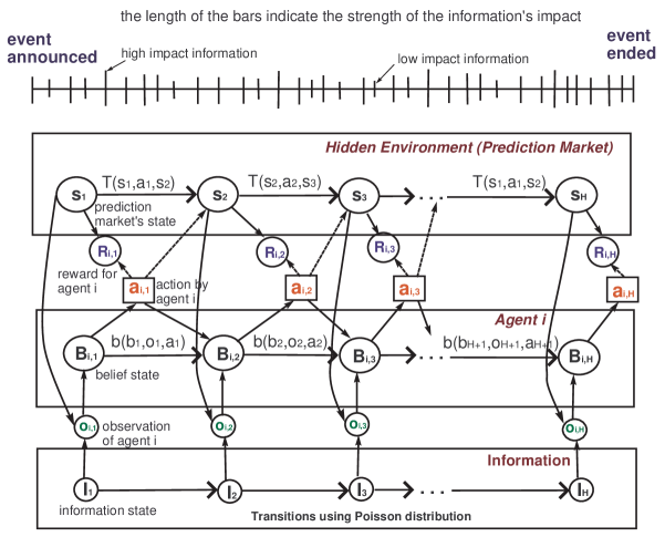
Figure 2: An agent interactions with the hidden environment (prediction market) and an external information source.

Based on the POSGI formulation of the prediction market, the interaction of an agent with the environment (prediction market) and the information source can be represented by the transition diagram shown in Figure 2. The environment (prediction market) goes through a set of states $\tilde{S}=\{s_{1},...,s_{H}\}:\tilde{S}\in S$, where $H$ is the duration of the event in the prediction market and $s_{h}$ represents the state of the market during trading period $h$. This state of the market is not visible to any agent. Instead, each agent $i$ has its own internal belief state $B_{i,h}$ corresponding to its belief about the actual state $s_{h}$. $B_{i,h}$ gives a probability distribution over the set of states $S$, where $B_{i,h}=(b_{1,h},...,b_{|S|,h})$. Consider trading period $h-1$ when the agents perform the joint action $\overline{a}_{h-1}$. Because of this joint action of the agents the environment stochastically changes to a new state $s_{h}$, defined by the state transition function $T(s_{h-1},a_{h-1},s_{h})$. There is also an external information state, $I_{h}$, that transitions to the next state $I_{h+1}$ given by the Poisson distribution [23] from which the information signal is sampled. The agent $i$ doesn’t directly see the environment state, but instead receives an observation $o_{i,S_{h}}=(\pi_{s_{h}},{\cal I}_{i,s_{h}})$, that includes the market price $\pi_{s_{h}}$ corresponding to the state $s_{h}$ as informed by the market maker, and the information signal ${\cal I}_{i,s_{h}}$. The agent $i$ then uses a belief update function to update its beliefs. Finally, agent $i$ selects an action using an action selection strategy and receives a reward $R_{i,s_{h}}$.

4.1 Trading agent belief update function

Recall from Section 4 that a belief state of a trading agent is a probability vector that gives a distribution over the set of states $S$ in the prediction market, i.e. $B_{i,h}=(b_{1,h},...,b_{|S|,h})$. A trading agent uses its belief update function $b:\Re^{\mid S\mid}\times A_{i}\times O_{i}\rightarrow\Re^{\mid S\mid}$ to update its belief state based on its past action $a_{i,h-1}$, past belief state $B_{i,h-1}$ and the observation $o_{i,S_{h}}$. The calculation of the belief update function for each element of the belief state, $b_{s^{\prime},h}$, $s^{\prime}\in S$, is described below:

$$b_{s^{\prime},h} = P(s^{\prime}|a_{i,h-1},o_{i})=\frac{P(s^{\prime},a_{i,h-1},o_{i},)}{P(a_{i,h-1},o_{i})}$$ (1)

$$= \frac{P(o_{i}|s^{\prime},a_{i,h-1})\cdot P(s^{\prime},a_{i,h-1})}{P(o_{i}|a_{i,h-1})P(a_{i,h-1})}$$

Because $a_{i,h-1}$ is conditionally independent given $s^{\prime}$ and $o_{i}$ is conditionally independent given $a_{i,h-1}$, we can rewrite Equation 1 as:

$$b_{s^{\prime},h}=\frac{P(o_{i}|s^{\prime})\cdot P(s^{\prime},a_{i,h-1})}{P(o_{i})P(a_{i,h-1})}=$$ (2)

$$\frac{\sum_{\iota\in\cal I}P(\iota)P(o_{i}|s^{\prime},\iota)\sum_{s\in S}P(s)P(s^{\prime}|s,a_{i,h-1})P(a_{i,h-1})}{P(o_{i})P(a_{i,h-1})}$$

$$= \frac{\sum_{\iota\in\cal I}P(\iota)P(o_{i}|s^{\prime},\iota)\sum_{s\in S}P(s)P(s^{\prime}|s,a_{i,h-1})}{P(o_{i})}$$

$$= \frac{\sum_{\iota\in\cal I}P(\iota)\Omega(s^{\prime},\iota,o_{i})\sum_{s\in S}T(s,a_{i,h-1},s^{\prime})b_{s,h-1}}{P(o_{i})}$$

All the terms in the r.h.s. of the Equation 2 can be calculated by an agent: $P(\iota)$ is the probability of receiving information signal $\iota$ and is available from the Poisson distribution [23] for the information arrival, $\Omega(s^{\prime},\iota,o_{i})$ is the probability of receiving observation $o_{i}$ in state $s^{\prime}$ when the information signal is $\iota$, $T(s,a_{i,h-1},s^{\prime})$ is the probability that the state $s$ transitions to state $s^{\prime}$ after agent $i$ takes action $a_{i,h-1}$, $b_{s,h-1}$ is the past belief of agent $i$ about state $s$, $P(o_{i})$ is the probability of receiving observation $o_{i}$, which is constant and can be viewed as a normalizing constant.

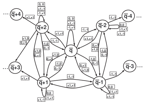
Figure 3: Finite state automata of the environment represented by the number of outstanding units of the security, $\overline{q}$, in the prediction market.

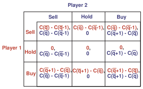
Figure 4: Two player normal form game in a state for which the number of outstanding shares is $\overline{q}$.

4.2 Trading agent action selection strategy

The objective of a trading agent in a prediction market is to select an action at each stage so that the expected reward that it receives is maximized. To understand this action selection process, we consider the decision problem facing each trading agent. Consider two agents whose available actions during each time step are to buy (=+1) or sell(=-1) only one unit of the security or not do anything (=0) by holding the security. Let the market state be denoted by $\overline{q}$, the number of purchased units of the security. Based on the set of actions available to each agent, the state can transition to one of the following states $\overline{q}+2$ (both agents buy), $\overline{q}+1$ (only one agent buys), $\overline{q}$ (both agents hold, or, one agent buys while the other agent sells, resulting in no transition), $\overline{q}+1$ (only agent sells), and $\overline{q}+2$ (both agents sell), as shown in Figure 3. We can expand this state space further by adding more states and transitions, but the number of states remains finite because the set of states $S$ of the POSGI is finite. Also, since the number of units of a security is finite, the number of transitions from a state is guaranteed to be bounded. We can construct a normal form game from this representation to capture the decision problem for each agent. The payoff matrix for this 2-player game at state $\overline{q}$ is shown in Figure 4. From this payoff matrix, we can use game-theoretic analysis to determine equilibrium strategies for each trading agent and find the actions that maximize its expected reward, as described below.

4.3 Correlated Equilibrium (CE) calculation

In the POSGI, the aggregated price information received by a trading agent from the market maker can be treated as a recommendation signal for selecting the agent’s strategy. This situation lends itself to a correlated equilibrium (CE) [1] where a trusted external agent privately recommends a strategy to play to each player. A CE is more preferred to the Nash or Bayesian Nash equilibrium because it can lead to improved payoffs, and it can be calculated using a linear program in time polynomial in the number of agents and number of strategies.

Each agent $i$ has a finite set of strategy profiles, $\Phi_{i}$ defined over its action space $A_{i}$. The joint strategy space is given by $\Phi=\prod_{i=1}^{|N|}\Phi_{i}$ and let $\Phi_{-i}=\prod_{j\neq i}\Phi_{j}$. Let $\phi\in\Phi$ denote a strategy profile and $\phi_{i}$ denote player $i$’s component in $\phi$. The utility received by each agent $i$ corresponds to its payoff or reward and is given by the agent $i$’s utility function $u_{i}(\phi)=R_{i}$ (for legibility we have dropped state $k$, but the same calculation applies at every state). A correlated equilibrium is a distribution $p$ on $\Phi$ such that for all agents $i$ and all strategies $\phi_{i},\phi_{i}^{\prime}$ if all agents follow a strategy profile $\phi$ that recommends player $i$ to choose strategy $\phi_{i}$, agent $i$ has no incentive to play another strategy $\phi_{i}^{\prime}$ instead. This implies that the following expression holds: $\sum_{\phi_{-i}\in\Phi_{-i}}p(\phi)(u_{i}(\phi)-u_{i}(\phi_{i}^{\prime},\phi_{-i}))\geq 0$, $\forall i\in N$, $\forall\phi_{i},\phi_{i}^{\prime}\in\Phi_{i}$ and where $u_{i}(\phi^{\prime}_{i},\phi_{-i})$ is the utility that agent $i$ gets when it changes its strategy to $\phi^{\prime}_{i}$ while all the other agents keep their strategies fixed at $\phi_{-i}$ and $p(\phi)$ is the probability of realizing a given strategy profile $\phi$.

Theorem 1.

A correlated equilibrium exists in our POSGI-based prediction market representation at each stage (trading period).

Proof.

At each stage in our prediction market, we can specify the correlated equilibrium by means of linear constraints as given below:

$$\sum_{\phi_{-i}\in\Phi_{-i}}p(\phi)(u_{i}(\phi)-u_{i}(\phi_{i}^{\prime},\phi_{-i}))\geq 0,\forall i\in N,\forall\phi_{i},\phi_{i}^{\prime}\in\Phi_{i}$$ (3)

$$\sum_{\phi\in\Phi}p(\phi)=1,$$ (4)

$$p(\phi)\geq 0$$ (5)

Equation 3 states that when agent $i$ is recommended to select strategy $\phi_{i}$, it must get no less utility from selecting strategy $\phi_{i}$ as it would from selecting any other strategy $\phi_{i}^{\prime}$. Constraints 4 and 5 guarantee that $p$ is a valid probability distribution. We can rewrite the linear program specification of the correlated equilibrium above by adding an objective function to it.

$$\mbox{max }\sum_{\phi\in\Phi}p(\phi),\mbox{ or min }-\sum_{\phi\in\Phi}p(\phi)\mbox{ s.t.}$$ (6)

$$\sum_{\phi\in\Phi,\phi_{-i}\in\Phi_{-i}}p(\phi)(u_{i}(\phi)-u_{i}(\phi_{i}^{\prime},\phi_{-i}))\geq 0,$$ (7)

$$\phi\geq 0$$ (8)

Program 7 is either trivial with a maximum of $0$ or unbounded. Hoenselaar [16] proved that there is a correlated equilibrium if and only if Program 7 is unbounded. To prove the unboundedness we consider the dual problem of Equation 7 given in Equation 10.

$$\mbox{max }0,\mbox{ s.t.}$$ (9)

$$\sum_{\phi\in\Phi,\phi_{-i}\in\Phi_{-i}}p(\overline{\phi})[(u_{i}(\phi)-u_{i}(\phi_{i}^{\prime},\phi_{-i})]^{T}\leq-1$$ (10)

$$\overline{\phi}\geq 0$$ (11)

where for every $p(\overline{\phi})$ there is $p(\phi)$ such that $p(\phi)[(u_{i}(\phi)-u_{i}(\phi_{i}^{\prime},\phi_{-i})]p(\overline{\phi})=0$.

Also in [28], the authors showed that the problem given in Equation 10 is always infeasible. From operations research we know that when the dual problem is infeasible the primal problem is feasible and unbounded. This means that the primal problem from Equation 7 is always unbounded. We can then conclude that there is at least one correlated equilibrium in every trading period of the prediction market. ∎

The CE calculation algorithm used by the trading agents in our agent-based prediction market is shown in Algorithm 1. The calculation of the matrix values of the $U$ matrix must be done once for each of the $N$ agents. Using the ellipsoid algorithm [28] the computation of the utility difference $u_{i}(\phi)-u_{i}(\phi_{i},\phi_{-i})$ for each agent $i$ can be done in $|\Phi_{i}|^{2}$ time. Therefore, the time complexity of the CECalc algorithm during each trading period comes to $N\times|\Phi_{i}|^{2}$.

CECalc($D,\Phi$)

Input: $D,\Phi$ //$D$ is the duration of the market, $\Phi$ is the set of strategies

Output: $p$ //correlated equilibrium

foreach $t\leftarrow 0$ to $D$  do

      //do this in each trading period

       Let $U$ be the matrix consisting of the values of $(u_{i}(\phi)-u_{i}(\phi_{i},\phi_{-i}))$, $\forall i\in N,\phi\in\Phi,\phi_{-i}\in\Phi_{i}$

       $p_{t}^{\prime}\leftarrow$ getDualDistribution($\Phi,U$);

       $p_{t}\leftarrow$ solve for $p_{t}$ s.t. $p_{t}U^{T}p_{t}^{\prime}=0$;

       return $p_{t}$;

      

end foreach

GetDualDistribution($\Phi,U$)

Input: $\Phi,U$

Output: $\Delta$

$l=0;$

$p^{\prime}_{l}\in[0,1]$;

$\Delta=\{\}$;

while $U^{T}\cdot p_{l}^{\prime}\leq-1$ is feasible do

       $\Delta=\Delta+p_{l}^{\prime};$

       $p_{l+1}^{\prime}=p_{l}+\epsilon^{N}$; //increase all elements of $p^{\prime}$ by some small amounts from vector $\epsilon^{N}$

       $l++;$

      

end while

return $\Delta$;

Algorithm 1 Correlated Equilibrium Algorithm

4.4 Correlated Equilibrium with Trading Agents’ Risk Preferences

Incorporating the risk preferences of the trading agents is an important factor in prediction markets. For example, the erroneous result related to the non-correlation between the trader beliefs and market prices in a prediction market in [24] was because the risk preferences of the traders were not accounted for, as noted in [13]. This problem is particularly relevant for risk averse traders because the beliefs(prices) and risk preferences of traders have been reported to be directly correlated [10, 20]. In this section, we examine CE that provides truthful revelation incentives in the prediction market where the agent population has different risk preferences. The risk preference of an agent $i$ is modeled through a utility function called the constant relative risk aversion (CRRA). We use CRRA utility function to model risk averse agents because it allows to model the effect of different levels of risk aversion and it has been shown to be a better model than alternative families of risk modeling utilities [31]. It has been widely used for modeling risk aversion in various domains including economic domain [17], psychology [21] and in the health domain [2]. The CRRA utility function is given below:

$$u_{i}(R_{i}) = \frac{R_{i}^{1-\theta_{i}}}{1-\theta_{i}},\,\,\mbox{if}\,\theta_{i}\neq 1$$

$$= ln(R_{i}),\,\,\mbox{if}\,\theta_{i}=1$$

Here, $-1<\theta_{i}<1$ is called the risk preference factor of agent $i$ and $R_{i}$ is the payoff or reward to agent $i$ calculated using the LMSR [5]. When $R_{i}<0$, we may get a utility in the form of a complex number. In that case, we convert the complex number to a real number by calling an existing function that uses magnitude and the angle of the complex number for conversion. For a risk neutral agent, $\theta_{i}=0$, which makes $u_{i}=R_{i}$, as we have assumed for our CE analysis of the risk neutral agent in Section 4.3. For risk averse agents, $\theta_{i}>0$. This makes the CRRA utility function concave. But the concave structure of the utility $u_{i}$ for a risk averse agent does not affect the existence of at least one correlated equilibrium because the unboundedness of Equation 7 is not affected by the concave structure of $u_{i}$. However, the equilibrium obtained with the risk averse utility function can be different from the one obtained with the risk neutral utility function - because the best response $p(\phi)$ to $p(\phi_{-i})$ calculated with the risk neutral utility function might not remain the best response when the agents are risk averse and use the risk averse utility function. To find a correlated equilibrium $p(\phi)$ in the market with risk averse agents, we first characterize the set of all Pareto optimal strategy profiles. A strategy profile $\phi^{P}$ is Pareto optimal if there does not exist another strategy profile $\phi^{\prime}$ such that $u_{i}(\phi^{\prime})\geq u_{i}(\phi^{P})$ $\forall i\in N$ with at least one inequality strict. In other words, a Pareto optimal strategy profile is one such that no trader could be made better off without making someone else worse off. A Pareto optimal strategy profile can be found by maximizing weighted utilities

$$max_{\phi}\sum_{i=1}^{|N|}\lambda_{i}u_{i}(\phi)\mbox{ for some }\lambda_{i}$$ (12)

Setting $\lambda_{i}=1$ for all $i\in N$ gives a utilitarian social welfare function. The maximization problem in Equation 12 can be solved using the Lagrangian method. We get the following system of $|N|$ equations:

$$\sum_{i=1}^{|N|}\lambda_{i}\frac{u_{i}(\phi)}{\phi_{i}}=0\mbox{ , }\forall j=1,...,|N|$$ (13)

that must hold at $\phi^{P}$. Each of these equations is obtained by taking a partial derivative of the respective agent’s weighted utility with respect to respective agent’s strategy profile, thus solving the maximization problem given in Equation 12. By solving the system of equations 13 we get the set of Pareto optimal strategy profiles. To determine if $p(\phi)$ is a correlated equilibrium we simply check whether it satisfies correlated equilibrium constraints for Pareto optimal strategy profile given below:
$\sum_{\phi_{-i}\in\Phi_{-i}}p(\phi)(u_{i}(\phi)-u_{i}(\phi_{i}^{\prime},\phi_{-i}))\geq 0,\forall i\in N,\forall\phi_{i},\phi_{i}^{\prime}\in\Phi_{i}$

Proposition 1.

If $p$ is a correlated equilibrium and $\phi^{P}$ is a Pareto optimal strategy profile calculated by $p$ in a prediction market with risk averse agents, then the strategy profile $\phi^{P}$ is incentive compatible, that is each agent is best off reporting truthfully.

Proof.

We prove by contradiction. Suppose that $\phi^{P}$ is not an incentive compatible strategy, that is, there is some other $\phi^{\prime}$ for which

$$u_{i}(\phi^{\prime})\geq u_{i}(\phi^{P})$$ (14)

Equation 14 violates two properties of $\phi^{P}$. First of all, since $\phi^{P}$ is Pareto optimal, we know that Equation 14 is not true, since $u_{i}(\phi^{P})\geq u_{i}(\phi^{\prime})$ by the definition of Pareto optimal strategy profile. Secondly, if we rewrite Equation 14 as $u_{i}(\phi^{P})-u_{i}(\phi^{\prime})\leq 0$ and multiply both sides by $p(\phi^{P})$, we get $p(\phi^{P})[u_{i}(\phi^{P})-u_{i}(\phi^{\prime})]\leq 0$. Since $p$ is a correlated equilibrium this inequality can not hold, otherwise it would violate the definition of the correlated equilibrium. ∎

5 Experimental Results

We have conducted several simulations using our POSGI prediction market. The main objective of our simulations is to test whether there is a benefit to the agents to follow the correlated equilibrium strategy. We do this by analyzing the utilities of the agents and the market price. The default values for the statistical distributions for market related parameters such as the number of days over which the market runs representing the duration of an event and the information signal arrival rate were taken from data obtained from the Iowa Electronic Marketplace(IEM) movie market for the event Monsters Inc. [19] and are shown in Table 1.

Name	Value
No. of days	$50$
Duration of $1$ day	$1sec$
No. of agents	$2$
No. of events	$1$
Max. allowed buy/sell quantity of security	$1$
Price of security	$[0,1]$

Table 1: Parameters used for our simulation experiments

For all of our simulations, we assume there is one event in the market with two outcomes (positive or negative); each outcome has one security associated with it. We consider events that are disjoint (non-combinatorial). This allows us to compare our proposed strategy empirically with other existing strategies while using real data collected from the IEM, which also considers non-combinatorial events. Since we consider disjoint events, having one event vs. multiple events does not change the strategic behavior of the agent or the results of each agent. We report the market price for the security corresponding to the outcome of the event being $1$ (event occurs).

We compare the trading agents’ and market’s behavior under various strategies employed by the agents. We use the following five well-known strategies for comparison [22] which are distributed uniformly over the agents in the experiments.

1. ZI (Zero Intelligence) - each agent submits randomly calculated quantity to buy or sell.

2. ZIP (Zero Intelligence Plus) - each agent selects a quantity to buy or sell that satisfies a particular level of profit by adopting its profit margin based on past prices.

3. CP (by Preist and Tol) - each agent adjusts its quantity to buy or sell based on past prices and tries to choose that quantity so that it is competitive among other agents.

4. GD (by Gjerstad and Dickhaut) - each agent maintains a history of past transactions and chooses the quantity to buy or sell that maximizes its expected utility.

5. DP (Dynamic Programming solution for POSG game) - each agent uses dynamic programming solution to find the best quantity to buy or sell that maximizes its expected utility given past prices, past utility, past belief and the information signal [14].

6. CE (Correlated equilibrium solution) - each agent uses Algorithm 1 from Section 4.3 to determine a correlated equilibrium strategy that gives a recommended quantity to buy or sell.

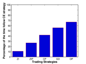
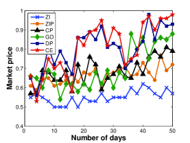
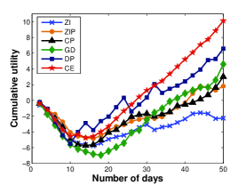
a	b	c

Figure 5: (a) Percentage of the number of days each compared trading strategy follows a correlated equilibrium strategy, (b) Market Prices, and, (c) Utilities of the risk neutral agent while using different trading strategies.

5.1 Risk-neutral Agents

For our first group of experiments we assume that the agents are risk neutral. First, we attempt to understand the correspondence between our CE strategy and each of the other compared strategies. For comparing the CE strategy with each strategy, we ran the simulations with identical settings, once with agents using the CE strategy for making trading decisions and then with the same agents using the compared strategy for making trading decisions. Figure 5(a) shows the number of times(days) an action recommended to a trading agent by the CE strategy is the same as the action recommended to a trading agent by one of the compared strategies, expressed as a percentage. We observe that the action recommended to a trading agent employing the ZI strategy is the same as the action recommended to a trading agent using CE strategy only $11\%$ of the time, while for the trading agent using the more refined DP strategy it is the same $68\%$ of the time. The higher percentage of adoption of the CE strategy by the more refined strategies indicates that the DP strategy is more sophisticated than simpler strategies.

In our next set of experiments, we compare the market prices and utilities obtained by a trading agent over time (days) while using different trading strategies. In each simulation run, the trading agent uses one of the compared strategies for determining its action at each time step (day). We compare the cumulative market prices and utilities for each such simulation. We report a scenario where the event in the prediction market happens and show the market prices and utilities for the security corresponding to the positive outcome of the event. In this scenario, the market price should approach $\$1$ (event happens) as the prediction market’s duration nears end. Figure 5(b) shows the market prices of the orders placed by the trading agents during the duration of the event for different strategies. We observe that agents using the CE strategy perform better since they are able to trade at prices that are closer to $\$1$, indicating that agents using the CE strategy are able to respond to other agents’ strategies and predict the aggregated price of the security more efficiently. This efficiency is further supported by the graph in Figure 5(c) that shows the utility of the agents while using different strategies. We see that the agents using the CE strategy are finally able to obtain $38\%$ more utility than the agents following the next best performing strategy (DP), and $85\%$ more utility than the agents following the second worst performing strategy (ZIP).

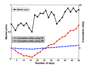
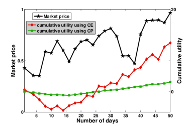
a	b

Figure 6: Comparison of the cumulative market prices and utilities obtained by: (a) CE and ZIP strategies, and, (b) CE and CP strategies.

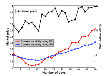
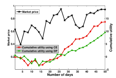
a	b

Figure 7: Comparison of the cumulative market prices and utilities obtained by: (a) CE and GD strategies, and, (b) CE and DP strategies.

For our following set of experiments, we further compare the CE strategy with other strategies by using two agents in the same simulation run - one agent using CE strategy and the other agent using the compared strategy. The results are reported in Figure 6 and 7. We can see that in each scenario the CE strategy outperforms other strategies. From Figures 6(a) and 7(b) respectively, we observe that the trading agent using CE strategy gets $95\%$ more utility than the trading agent using ZIP strategy and $41\%$ more utility than the trading agent using DP strategy. Overall, we can say that using the POSGI model allows the agent to avoid myopically predicting prices and use the correlated equilibrium to calculate prices more accurately and obtain higher utilities.

5.2 Risk averse Agents

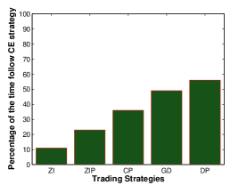
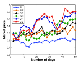
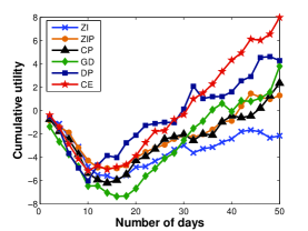
a	b	c

Figure 8: (a) Percentage of the number of days each compared trading strategy follows a correlated equilibrium strategy, (b) Market Prices, and, (c) Utilities of the risk averse agent while using different trading strategies.

Next, we conduct similar simulations for the market while using risk averse agents that use the risk averse utility function given in Section 4.4. Since in real world most people are risk averse, we ran several experiments with different values of the risk preference $\theta_{i}>0$. We report the results for $\theta_{i}=0.8$ (strongly risk averse trading agent) to see a better effect of the risk averse preference of trading agents on the market prices and their own utilities. To compare the CE strategy with each of the other strategies we ran the simulation with identical settings, once with risk averse agents using the CE strategy for making trading decision and then with the same risk averse agents using the compared strategy for making trading decisions. Figure 8(a) shows the number of times an action recommended to a risk averse trading agent by the CE strategy is the same as the action recommended to a risk averse trading agent by one of the compared strategies, expressed as a percentage. We can see that the risk averse agents employing any of the five compared strategies end up adopting the action that it the same as the action proposed by the CE strategy only $11-60\%$ of the time. We notice that the ZI agents are not affected by the risk averse behavior of the agents (they follow the CE strategy $11\%$ of the time when the agents are either risk averse or risk neutral) because they do not use their past utility to determine future prices. However, other compared agent strategies use their past utilities to predict future prices. The concave nature of the CRRA utility function with $\theta_{i}>0$ lowers the utilities that these agents receive, and, this results in these agents following the CE strategy less often. The effect of the lowered utility due to the risk averse (concave) utility function is also seen in Figures 8(b) and (c). Figures 8(b) shows the market prices for an event that has a final outcome $=1$. We again observe that the agents using CE strategy are able to predict the aggregated price of the security more efficiently during the duration of the event. Figure 8(c) that shows the utility of the risk averse agents while using different strategies. We see that the agents using the CE strategy are able to obtain $42\%$ more utility than the agents following the next best performing strategy (DP) and $127\%$ more utility than the agents following the worst performing strategy (ZI).

Strat.	Risk Neutral Agent			Risk Averse Agent
	$\%F_{CE}$	Price	Utility	$\%F_{CE}$	Price	Utility
ZI	$11\%$	$36\%$	$123\%$	$11\%$	$32\%$	$132\%$
ZIP	$26\%$	$25\%$	$85\%$	$22\%$	$26\%$	$89\%$
CP	$41\%$	$23\%$	$77\%$	$35\%$	$20\%$	$83\%$
GD	$47\%$	$19\%$	$52\%$	$39\%$	$16\%$	$58\%$
DP	$68\%$	$9\%$	$38\%$	$60\%$	$10\%$	$41\%$

Table 2: Percentage of the number of days each compared strategy follows the CE strategy ($\%FCE$ in cols. $2$ and $5$), the percentage of the difference between each compared strategy and the CE strategy for the market price (cols. $3$ and $6$) and utility (cols. $4$ and $7$). Results are shown for both risk neutral and risk averse trading agents.

The summary of all of our results is given in Table 2. For each type of agent, risk neutral or risk averse, the first column, $\%F_{CE}$, indicates percentage of the number of days the actions of the trading agents using each compared strategy are the same as the CE strategy. The second and the third column show the percentage of the difference between each compared strategy and the CE strategy for the market price and utility, respectively. In summary, the POSGI model and the CE strategy result in better price tracking and higher utilities because they provide each agent with a strategic behavior while taking into account the observations of the prediction market and the new information of the events.

6 Conclusions

In this paper, we have described an agent-based POSGI prediction market with an LMSR market maker and empirically compared different agent behavior strategies in the prediction market. We proved the existence of a correlated equilibrium in our POSGI prediction market with risk neutral agents, and showed how correlated equilibrium can be obtained in the prediction market with risk averse agents. We have also empirically verified that when the agents follow a correlated equilibrium strategy suggested by the market maker they obtain higher utilities and the market prices are more accurate.

In the future we are interested in conducting experiments in an $n$-player scenario for the POSGI formulation given in Section $3$ using richer commercially available prediction market data sets. We also plan to analyze the performance of the CE strategy in the scenarios where the outcome of the event does not correspond to the predicted outcome of the event by the market price, i.e. when prediction market fails. We also plan to investigate the dynamics evolving from multiple prediction markets that interact with each other. Finally, we are interested in exploring truthful revelation mechanisms that can be used to limit untruthful bidding in prediction markets.

References

- [1] R. J. Aumann. Subjectivity and correlation in randomized strategies. Journal of Math- ematical Economics, 1(1):67-96, 1974.
- [2] H. Bleichrodt, J. van Rijn, M. Johannesson. Probability weighting and utility curvature in QALY-based decision making. Journal of Mathematical Psychology, 43:238-260, 1999.
- [3] Y. Chen. Predicting Uncertain Outcomes Using Information Markets: Trader Behavior and Information Aggregation. New Mathematics and Natural Computation, 2(3):1-17, 2006.
- [4] Y. Chen, T. Mullen, C. Chu. An In-Depth Analysis of Information Markets with Aggregate Uncertainty. Electronic Commerce Research 2006; 6(2):201-22.
- [5] Y. Chen, D. Pennock. Utility Framework for Bounded-Loss Market Maker. Proc. of the 23rd Conference on Uncertainty in Articifial Intelligence (UAI 2007), pages 49-56, 2007.
- [6] Y. Chen, S. Dimitrov, R. Sami, D.M. Reeves, D.M. Pennock, R.D. Hanson, L. Fortnow, R. Gonen. Gaming Prediction Markets: Equilibrium Strategies with a Market Maker. Algorithmica, 2009.
- [7] B. Cowgill, J. Wolfers, E. Zitzewitz. Using Prediction Markets to Track Information Flows: Evidence from Google. Dartmouth College (2008); http://www.bocowgill.com/GooglePredictionMarketPaper.pdf.
- [8] S. Das. The Effects of Market-making on Price Dynamics. Proceedings of AAMAS 2008; 887-894.
- [9] S. Dimitrov and R. Sami. Nonmyopic Strategies in Prediction Markets. Proc. of the 9th ACM Conference on Electronic Commerece (EC), pages 200-209, 2008.
- [10] S. Dimitrov. Information Procurement and Delivery: Robustness in Prediction Markets and Network Routing. PhD Thesis, University of Michigan, 2010.
- [11] J. Feigenbaum, L. Fortnow, D. Pennock and R. Sami. Computation in a Distributed Information Market. Theor. Comp. Science, 343(1-2):114-132, 2005.
- [12] D. Fudenberg and J. Tirole. Game Theory. MIT Press, 1991.
- [13] S. Gjerstad. Risks, Aversions and Beliefs in Predictions Markets. mimeo, U. of Arizona, 2004.
- [14] E. Hansen, D. Bernstein, S. Zilberstein. Dynamic programming for partially observable stochastic games. In Proceedings of the 19th National Conference on Artificial Intelligence, pages 709-715, 2004.
- [15] R. Hanson. Logarithmic Market scoring rules for Modular Combinatorial Information Aggregation. Journal of Prediction Markets, 1(1):3-15, 2007.
- [16] A. Hoenselaar. Equilibria in Multi-Player Gamesequilibria. 2007. http://www.cs.brown.edu/courses/cs244/notes/andreas.pdf.
- [17] C.A. Holt, S.K. Laury. Risk aversion and incentive effects. American Economic Review, 92:1644-1655, 2002.
- [18] K. Iyer, R. Johari, C. Moallemi. Information Aggregation in Smooth Markets. Proceedings of the 11th ACM conference on Electronic commerce (EC’10), pages 199-206, 2010.
- [19] Iowa Electronic Marketplace. URL: www.biz.uiowa.edu/iem/
- [20] J.B. Kadane and R.L.Winkler. Separating probability elicitation from utilities. Journal of the American Statistical Association, 83(402):357-363, 1988.
- [21] R.D. Luce, C.L. Krumhansi. Measurement, scaling, and psychophysics. In Stevens Handbook of Experimental Psychology, Wiley: New York, 1:3-74, 1988.
- [22] H. Ma, H. Leung. Bidding Strategies in Agent-Based Continuous Double Auctions. Whitestein Series In Software Agent Technologies And Autonomic Computing, 2008.
- [23] J. Maheu, T. McCurdy. New Arrival Jump Dynamics, and Volatility Components for Individual Stock Returns. The Journal of Finance, 59(2):755-793, 2004.
- [24] C. Manski. Interpreting the Predictions of Prediction Markets. Economic Letters, 91(3):425-429, 2006.
- [25] M. Ostrovsky. Information Aggregation in Dynamic Markets with Strategic Traders. Proc. of the 10th ACM conference on Electronic commerce (EC’09), pages 253-254, 2009.
- [26] A. Othman and T. Sandholm. Automated Market Making in the Large: The Gates Hillman Prediction Market. of the 11th ACM conference on Electronic commerce (EC’10), pages 367-376, 2010.
- [27] A. Othman, T. Sandholm, D. Reeves and D. Pennock. A Practical Liquidity-Sensitive Automated Market Maker. of the 11th ACM conference on Electronic commerce (EC’10), pages 377-386, 2010.
- [28] C. Papadimitriou, T. Roughgarden. Computing correlated equilibria in multi-player games. Journal of ACM, 55(3):1-29, 2008.
- [29] C. Plott and K. Chen. Information Aggregation Mechanisms: Concept, Design and Implementation for a Sales Forecasting Problem. Social Science working paper no. 1131, California Institute of Technology, 2002.
- [30] A. Tversky and D. Kahneman. The framing of decisions and the psychology of choice. Science, 211:453-458, 1981.
- [31] P.P. Wakker. Explaining the Characteristics of the Power (CRRA) Utility Family, Health Economics, 17:1329-1344, 2008.
- [32] J. Wolfers and E. Zitzewitz. Prediction Markets. Journal of Economic Perspectives, 18(2):107-126, 2004.
- [33] J. Wolfers and E. Zitzewitz. Interpreting Prediction Markets as Probabilities. NBER Working Paper No. 12200, May 2006.
- [34] Yootles. URL: http://www.yootles.com