Branched projective structures with quasi-Fuchsian holonomy

Abstract.

We prove that if $S$ is a closed compact surface of genus $g\geq 2$, and if $\rho:\pi_{1}(S)\rightarrow\mathrm{PSL}(2,\mathbb{C})$ is a quasi-Fuchsian representation, then the deformation space $\mathcal{M}_{k,\rho}$ of branched projective structures on $S$ with total branching order $k$ and holonomy $\rho$ is connected, as soon as $k>0$. Equivalently, two branched projective structures with the same quasi-Fuchsian holonomy and the same number of branch points are related by a movement of branch points. In particular grafting annuli are obtained by moving branch points. In the appendix we give an explicit atlas for $\mathcal{M}_{k,\rho}$ for non-elementary representations $\rho$. It is shown to be a smooth complex manifold modeled on Hurwitz spaces.

1. Introduction

A $\mathbb{C}\mathbb{P}^{1}$-structure on a surface is a geometric structure modeled on the Riemann sphere and its group of holomorphic automorphisms, identified with $\mathrm{PSL}(2,\mathbb{C})$. A chart of a $\mathbb{C}\mathbb{P}^{1}$-structure can be developed (i.e. continued with the use of charts) to a map defined on the universal cover of the surface, which is equivariant with respect to a certain representation of the fundamental group of the surface to $\mathrm{PSL}(2,\mathbb{C})$, called the holonomy. This is well-defined up to composition by inner automorphisms of $\mathrm{PSL}(2,\mathbb{C})$. Such a $\mathbb{CP}^{1}$-structure will be referred to as projective structure.

Projective structures were introduced by studying second order ODE’s, with applications to the uniformization theorem, which states that the universal cover of every Riemann surface is biholomorphic to either $\mathbb{CP}^{1}$, $\mathbb{C}$, or $\mathbb{H}^{2}$ corresponding to whether the Euler characteristic is positive, zero or negative. The composition of the said biholomorphism with the natural inclusion in $\mathbb{CP}^{1}$ defines a developing map of a projective structure on the topological surface whose holonomy representation is the identification of the fundamental group with a subgroup of automorphisms of the uniformized covering map, which lies in $\mathrm{PSL}(2,\mathbb{C})$ in either case. In particular, hyperbolic structures on closed surfaces are examples of $\mathbb{CP}^{1}$-structures: the developing map takes its values in the upper-half plane model of $\mathbb{H}^{2}$ — viewed as a subset of $\mathbb{CP}^{1}$ — and the holonomy in a discrete co-compact subgroup of $\mathrm{PSL}(2,\mathbb{R})<\mathrm{PSL}(2,\mathbb{C})$. In general the holonomy of a $\mathbb{CP}^{1}$-structure on a closed surface $S$ is said to be Fuchsian if it is faithful and its image is conjugated to a discrete co-compact subgroup of $\mathrm{PSL}(2,\mathbb{R})$. For such a representation we can always consider the corresponding hyperbolic structure on $S$ which is called the uniformizing structure. A representation is called quasi-Fuchsian if it is topologically conjugated to a Fuchsian representation when acting on the Riemann sphere.

In the 70’s, some exotic $\mathbb{C}\mathbb{P}^{1}$-structures with quasi-Fuchsian holonomy were discovered (see [12],[27],[30]). More precisely, given a $\mathbb{C}\mathbb{P}^{1}$-structure, there is a surgery called grafting, which enables to produce a different projective structure without changing its holonomy. A grafting of the uniformizing structure along a simple closed curve $\gamma$ is the result of cutting $S$ along $\gamma$ and gluing back a flat annulus of an appropriate modulus. In [7], Goldman showed that any projective structure with quasi-Fuchsian holonomy is obtained by grafting the uniformizing structure along a multi-curve .

In particular, this implies that the set of projective structures with the same quasi-Fuchsian holonomy is discrete. Baba recently extended Goldman’s result to the case where the holonomy is a generic representation in $\mathrm{Hom}(\pi_{1},\mathrm{PSL}(2,\mathbb{C}))$, see [2].

In this paper, we are interested in branched projective structures on closed orientable surfaces. These are given by atlas where local charts are finite branched coverings and transition maps lie in $\mathrm{PSL}(2,\mathbb{C})$. Such structures arise naturally in many contexts. For instance in the theories of conical $\mathbb{H}^{2}$-structures, of branched coverings, of locally flat projective connections or of transversally projective holomorphic foliations (more details are given later in this introduction and in sections 2 and 12). As in the unbranched case, a chart can be continued to define a developing map on the universal cover of the surface equivariant with respect to a holonomy representation of the fundamental group of the surface in $\textrm{PSL}(2,\mathbb{C})$. In the spririt of Goldman’s theorem we give an explicit construction of any branched projective structure with quasi-Fuchsian holonomy by elementary surgeries that preserve the holonomy. These new surgeries can be varied continuously and allow to define a topology on the set $\mathcal{M}_{k,\rho}$ of branched projective structures with fixed holonomy $\rho:\pi_{1}(S)\rightarrow\mathrm{PSL}(2,\mathbb{C})$ and total branching order $k$ on a marked surface $S$ of genus $g$. We show that, unlike in the unbranched case, for quasi-Fuchsian $\rho$ and $k>0$, the deformation space is connected.

Theorem 1.1 (Main result).

Let $S$ be a compact oriented closed surface. Every branched projective structure with quasi-Fuchsian holonomy on $S$ having at least one branch point is obtained from a uniformizing structure by bubblings and moving branch points. Equivalently, if $k>0$ and $\rho:\pi_{1}(S)\rightarrow\mathrm{PSL}(2,\mathbb{C})$ is a quasi-Fuchsian representation, then the deformation space $\mathcal{M}_{k,\rho}$ is non-empty if and only if $k$ is even, and in this case it is connected if $k>0$.

Let us define the elementary surgeries and the topology on $\mathcal{M}_{k,\rho}$ properly.

Bubbling a given branched projective structure consists in cutting the surface along an embedded arc $\gamma$ whose image by the developing map is an embedded arc $\eta\subset\mathbb{CP}^{1}$, and gluing the disc $\mathbb{CP}^{1}\setminus\eta$ endowed with the canonical projective structure. Obviously, the topology of the surface does not change nor does the holonomy representation. At the endpoints of $\gamma$ the new branched projective structure has two branch points. By bubbling several arcs we can produce examples of branched projective structures with any even number of simple branch points.

Moving a branch point is a local surgery that allows to change the position of a branch point, collapse two or more branch points or split a non-simple branch point into several branch points of lower branching order. In either case the holonomy of the resulting projective structure remains fixed and the total order of the branching divisor too. This surgery is a particular case of a Schiffer variation and allows to understand the local topology of $\mathcal{M}_{k,\rho}$.

Gallo-Kapovich-Marden [6, Problem 12.1.2, p. 700] asked whether any couple of branched projective structures with the same holonomy are related by a sequence of elementary operations: grafting, degrafting, bubbling and debubbling. For quasi-Fuchsian representations Theorem 1.1 gives a positive answer by replacing the elementary operations by: bubbling, debubbling and moving branch points. The connectedness of $\mathcal{M}_{k,\rho}$ and a continuity argument shows that the answer to their original question is positive for $k=2$. We believe that the argument generalizes for bigger $k$.

It is worth pointing out that in full generality the spaces $\mathcal{M}_{k,\rho}$ are not necessarily connected. For instance, consider $\rho$ to be the holonomy of a hyperbolic metric with two conical points of angle $4\pi$ on a compact surface of genus bigger than two. It can be thought as a branched projective structure whose developing map has image in $\mathbb{H}^{2}$. On the other hand we can construct examples with the same holonomy and branching order by doing a bubbling to a $\mathbb{CP}^{1}$-structure with holonomy $\rho$ –which exists by applying [6]– and this time the developing map is surjective onto $\mathbb{CP}^{1}$. Since this last property is stable under moving branch points the two projective structures lie in different connected components of $\mathcal{M}_{2,\rho}$ (see [31], [25] and [26] for related arguments).

Another interesting example is the case where $\rho$ is the trivial representation. The deformation spaces $\mathcal{M}_{k,\rho}$ are then the so-called Hurwitz spaces, namely the moduli spaces of branched coverings over $\mathbb{C}\mathbb{P}^{1}$. Since Clebsch and Hurwitz we know that these spaces are connected (see for instance [11] and the more recent generalizations in [19]).

Let us focus on the surgery operations that preserve the holonomy defined so far. Remark that bubbling adds two branch points, moving branch points does not change the total branching order, and grafting does not involve branch points at all. However, these surgeries relate to each other in interesting ways. Simple examples of such relations can be easily produced: a bubbling followed by local movement of branch points can be still interpreted as a bubbling, $k$ consecutive bubblings are related by moving branch points independently of the order and arcs where we bubble (see Corollaries 2.10 and 2.11). One of the most striking relations between bubbling and grafting is:

Theorem 1.2.

Over a given branched projective structure a bubbling followed by a debubbling can produce any grafting on a simple closed curve.

It immediately implies one of the key pieces for the proof of Theorem 1.1, namely that by moving branch points we can produce any grafting annulus. We point out that there are no restrictions on the holonomy representation in Theorem 1.2.

As will be explained in next subsection, our initial motivation was to study holomorphic curves of general type in a class of non-Kähler threefolds, and the problem led us to a question on the existence of rational curves in $\mathcal{M}_{k,\rho}$. Tan observed (in [31]) that each $\mathcal{M}_{k,\rho}$ admits a complex structure. However, the obvious generalization of the complex structure defined in the absence of branch points presents some subtleties that we want to point out.

It is well known that the space of unbranched projective structures on a given compact orientable surface has a natural complex structure by using the Schwarzian derivative of developing maps. In fact it is an affine bundle over Teichmüller space whose fibers are affine spaces over the vector space of holomorphic quadratic differentials. Its direct generalization to branched projective structures does not have such a regular structure. For a branched projective structure we can still define its underlying complex structure and determine a point in Teichmüller space. At a branch point of the developing map we can calculate the Schwarzian derivative with respect to the uniformizing coordinate of the complex structure. It presents a pole of order two regardless of the order of branching. In fact it is the coefficient of the lowest term in the Laurent series that gives the order of branching. For functions with this type of development there are even some extra algebraic conditions on the coefficients to be satisfied to guarantee that the inversion of the Schwarzian operator produces a holomorphic germ (as opposed to a pole or logarithmic pole). When we want to allow to collapse two different branch points we have a discontinuity in the lowest coefficient of the series (see the Appendix for more details). The spaces $\mathcal{M}_{k,\rho}$ are subspaces of this “singular complex space” bundle. Nevertheless, in the spirit of the topology defined by moving branch points, the spaces $\mathcal{M}_{k,\rho}$ –where $\rho$ is non-elementary– admit a natural complex manifold structure of dimension $k$. The subject is discussed in detail for future reference in the Appendix.

1.1. Additional remarks and open problems

Determining all components of $\mathcal{M}_{k,\rho}$ seems interesting in general. In some cases we can identify special components. For instance, when the holonomy representation $\rho$ is purely loxodromic, all branched projective structures obtained by bubbling (unbranched) $\mathbb{CP}^{1}$-structures with the given holonomy, belong to the same connected component. Indeed, by Baba’s theorem [2], Theorem 1.2, and Corollary 2.10 we can join any pair of such structures by a movement of branch points. As was said before, sometimes it is not the unique connected component.

The next challenging problem is to understand the higher homology/homotopy groups of the deformation spaces $\mathcal{M}_{k,\rho}$ when $\rho$ is quasi-Fuchsian. These spaces are all homeomorphic if we fix the genus of the underlying surface and $k$ (see Proposition 11.1). The understanding of the second homotopy group of $\mathcal{M}_{k,\rho}$ has a strong relation with monodromies of linear differential equations on curves and more precisely, to the Riemann Hilbert problem. Namely, consider a differential equation of the form

(1) $$dv=\omega\cdot v$$

where $S$ is a complex algebraic curve, $\omega$ is a given $1$-form over $S$ with values in the Lie algebra $sl(2,\mathbb{C})$, and $v:S\rightarrow\mathbb{C}^{2}$ is a holomorphic map. The Riemann-Hilbert problem consists in characterizing the representations arising as the monodromy of the solutions of an equation of type (1). For instance, it is not known whether a non-trivial real monodromy is possible.

If $g$ is the genus of $S$ and $\rho$ is the monodromy of (1), then the deformation space $\mathcal{M}_{2g-2,\rho}$ has a non trivial second homotopy group. This is because for each initial value, the solution $v$ of (1) defines a branched projective structure on $S$ with monodromy $\rho$, whose total branching order is easily seen to be $2g-2$. The resulting rational curve in $\mathcal{M}_{k,\rho}$ projects to a rational curve in the moduli space of branched projective structures, whose homological class is non-trivial, since the moduli space is Kähler. Hence, proving that $\mathcal{M}_{2g-2,\rho}$ has trivial second homotopy group would prove that $\rho$ does not appear as the monodromy of an equation of type (1).

This problem is also related to the study of holomorphic curves in the non algebraic manifolds $\Gamma\backslash\mathrm{SL}(2,\mathbb{C})$ where $\Gamma$ is a lattice in $\mathrm{SL}(2,\mathbb{C})$. This space can be thought as the space of orthonormal frames on a hyperbolic $3$-manifold (see [8]). If we have a solution of (1) whose monodromy lies in a lattice $\Gamma$ of $\mathrm{SL}(2,\mathbb{C})$, then the matrix formed by two independent solutions of (1) defines a curve isomorphic to $S$ in the quotient. We mention here that Huckleberry and Margulis proved that there is no complex hypersurface in such a complex manifold, see [14].

More generally, one could ask whether $\mathcal{M}_{k,\rho}$ is a $K(\pi,1)$ when $\rho$ is quasi-Fuchsian. This problem can be compared to a problem of Kontsevich-Zorich on the topology of connected components of the moduli space of translation surfaces (which are particular branched projective structures), see [18] and the list of problems [13].

1.2. Structure of the paper

After introducing the basic concepts and tools for branched projective structures in section 2, we analyze some special properties of those having Fuchsian holonomy in Sections 3 and 4. Then we proceed to prove Theorem 1.2.

The proof of the main theorem is carried first under the hypothesis of Fuchsian holonomy. To generalize to quasi-Fuchsian representations, we prove that the space $\mathcal{M}_{k,\rho}$ is homeomorphic to some $\mathcal{M}_{k,\rho^{\prime}}$ where $\rho^{\prime}$ is Fuchsian (see Proposition 11.1).

After Theorem 1.2 the proof reduces to an induction argument that shows that, after moving branch points of a given branched projective structure, it coincides with a finite number of bubblings on a (possibly exotic) $\mathbb{CP}^{1}$-structure. This argument takes up most of the paper and we have split it into different steps in Sections 6 to 11. As we mentioned before, there is an Appendix where we describe the complex structure of the deformation space $\mathcal{M}_{k,\rho}$, providing an explicit atlas modeled on Hurwitz spaces. Other parameterisations of $\mathcal{M}_{k,\rho}$ are also discussed.

Let us comment further on the details of the inductive argument. What we prove is that given a branched projective structure with Fuchsian holonomy, we can move the branch points so that the structure can be debubbled. Since debubbling decreases the number of branch points by $2$, after a finite number of debubblings we find an unbranched projective structure, hence it is a grafting over a multi-curve of the uniformizing structure by Goldman’s theorem.

We use the point of view of Faltings ([5]) and Goldman ([7]), that is, for a branched projective structure with Fuchsian holonomy we look at the decomposition of the surface obtained as the pull-back of the $\mathrm{PSL}(2,\mathbb{R})$-invariant decomposition of the Riemann sphere $\mathbb{C}\mathbb{P}^{1}=\mathbb{H}^{+}\cup\mathbb{R}\mathbb{P}^{1}\cup\mathbb{H}^{-}$, where $\mathbb{H}^{\pm}$ are the upper and lower half planes. The components of the positive and negative parts inherit a branched hyperbolic structure, i.e. a conical hyperbolic metric. Coarse properties of these metrics are explained in Section 3, where peripheral geodesics and peripheral annuli are defined. Most of the work consists in understanding the geometry of these components in detail, especially that of the peripheral geodesics.

Some topological invariants of the decomposition in positive and negative components are described by an index formula which we prove by closely following the ideas of Goldman’s thesis (see Section 4).

To begin moving branch points, we first need to know how and where one can move them. Sections 6 and 8 provide sufficient conditions to move branch points. In particular, in Section 8 we deal with possible degenerations to nodal curves when two branch points collide.

The next step of the proof is to reduce to the case where all the branch points belong the positive part (see Section 9). The index formula then tells us that there exist some negative discs isomorphic to a hyperbolic plane.

After that we are able to prove that the peripheral geodesic of the juxtaposed component of some negative disc, has a simple topology, namely, it is a bouquet of at most three circles. This is done by moving the branch points belonging to a positive component to a single branch point (see Section 10). We then invoke a result proved in Section 7 by a direct case by case analysis, which says that the structure can be debubbled.

One of the cases we have to deal with is a particular configuration that we called the “triangles”. They constitute an especially interesting instance and we discuss an example in detail in subsection 3.5.

The main technical tool that is used along the way is the notion of embedded twin paths for a branched projective structures. These allow us to move in each component of the deformation space of branched projective structures.

1.3. Acknowledgments

We are pleased to thank Shinpei Baba, Francesco Bonsante, Bill Goldman, Misha Kapovich, Cyril Lecuire, Samuel Lelièvre, Frank Loray, Peter Makienko, Luca Migliorini, Gabriele Mondello, Joan Porti and Ser Peow Tan for interesting discussions along the elaboration of the paper.

We are grateful to the following institutions for the very nice working conditions provided: CRM Barcelona, Institut Henri Poincaré, Mittag-Leffler Institute, Orsay, Pisa University, Universidade Federal Fluminense (UFF).

G. Calsamiglia’s research is supported by CNPq/FAPERJ and CAPES-Mathamsud; B. Deroin’s by the ANR projects: 08-JCJC-0130-01, 09-BLAN-0116, and received support from the Brazil - France cooperation agreement. S. Francaviglia’s research received support from UFF.

2. Definitions and preliminaries

2.1. Branched projective structures (BPS)

For $g\geq 2$ let $\Gamma_{g}$ be a group isomorphic to the fundamental group of a closed surface of genus $g$. A marked surface of genus $g$ is an oriented closed surface $S$ of genus $g$ together with the data of a universal cover $\pi:\widetilde{S}\rightarrow S$ and an identification of $\Gamma_{g}$ with the covering group of $\pi$.

Definition 2.1.

A branched projective structure (in short BPS) on a marked surface $S$ is a maximal atlas whose charts are finite-sheeted, orientation preserving, branched coverings over open subsets of $\mathbb{CP}^{1}$, and such that the transition functions belong to $\mathrm{PSL}(2,\mathbb{C})$. We identify two structures if there is a projective (in local charts) diffeomorphism which lifts to a $\Gamma_{g}$-equivariant diffeomorphism between the universal covers.

A BPS induces a complex structure and thus angles on $S$. Unbranched points are called regular, the total angle around them is $2\pi$. The cone-angle around branch points is $2\pi$ times the branch-order.

Given a BPS on a marked surface $S$, every local chart can be extended to a projective map $D:\widetilde{S}\to\mathbb{CP}^{1}$, which is equivariant w.r.t. a representation $\rho:\pi_{1}(S)\to\mathrm{PSL}(2,\mathbb{C})$:

$$D(\gamma x)=\rho(\gamma)D(x)\qquad\forall x\in\widetilde{S},\gamma\in\pi_{1}(S).$$

The map $D$ is well-defined up to left-composition by elements of $\mathrm{PSL}(2,\mathbb{C})$. Any representative of its $\mathrm{PSL}(2,\mathbb{C})$-left class is called a developing map for the structure and the representation $\rho$ is called the holonomy of the developing map. If $D_{1}$ and $D_{2}=\varphi\circ D_{1}$ are two developing maps for the same structure, then the corresponding representations are related by

$$\rho_{2}=\varphi\rho_{1}\varphi^{-1}.$$

The conjugacy class of the holonomy representation is called the holonomy of the structure. Note that if the holonomy has trivial centraliser– for intance if its image is a non-elementary group– then once a representative in the conjugacy class of the holonomy has been fixed, there is only one developing map for the structure with that holonomy.

In the present paper we are interested in studying projective structures having a fixed holonomy with some prescribed properties. In particular we will treat the Fuchsian case. In the literature a Fuchsian group is a discrete subgroup of ${\rm PSL}(2,\mathbb{R})$.

Definition 2.2.

Let $S$ be an oriented closed surface and $\rho:\pi_{1}(S)\to{\rm PSL}(2,\mathbb{C})$ a representation. We say $\rho$ is Fuchsian if it is faithful, its image is conjugated to a discrete subgroup $\Gamma$ of ${\rm PSL}(2,\mathbb{R})$ with no parabolic nor elliptic elements other than the identity and there exists a $\rho$-equivariant diffeomorphism between $\widetilde{S}$ and $\mathbb{H}^{2}$ preserving the orientation.

2.2. Examples

The first obvious examples are complete hyperbolic structures: under the natural inclusion $\textrm{Aut}(\mathbb{H}^{2})\hookrightarrow\textrm{Aut}(\mathbb{C}\mathbb{P}^{1})$, any hyperbolic structure on a closed surface can be considered as a $\mathbb{C}\mathbb{P}^{1}$-structure, having no branch points and Fuchsian holonomy.

Definition 2.3 (Uniformizing structures).

Let $S$ be a closed surface of genus at least two, and $\rho:\pi_{1}(S)\to{\rm PSL}(2,\mathbb{C})$ be a Fuchsian representation. The uniformizing structure on $S$ is the projective structure induced by the hyperbolic metric on $S$ with holonomy $\rho$.

Next, we have branched coverings. Let $S$ be a compact hyperbolic surface and $S_{1}\rightarrow S$ be a branched covering. By pulling back the atlas of the uniformizing structure of $S$ we get a branched projective structure on $S_{1}$. In general the holonomy of $S_{1}$ is not Fuchsian.

More interesting examples are produced by considering holomorphic singular codimension one transversely projective foliations on complex manifolds. Such foliations satisfy that the changes of coordinates of the foliated charts can be written as $(x,z)\mapsto(h(x,z),\varphi(z))$ for some $\varphi\in\textrm{PSL}(2,\mathbb{C})$. The foliated charts of a transversely projective foliation $\mathcal{F}$ on a manifold $M$ induce a branched projective structure on any Riemann surface $S\subset M$ that avoids the singular set of $\mathcal{F}$ and is generically transverse to $\mathcal{F}$. It suffices to restrict the local projections $(x,z)\mapsto z$ to $S$. At the points of tangency between $S$ and $\mathcal{F}$ we obtain branch points for the induced BPS on $S$. Transversely projective foliations have been extensively studied and some accouts can be found in [21], [28] and [32]. A particularly interesting and important family of examples are regular holomorphic foliations on $\mathbb{CP}^{1}$-bundles $B\rightarrow S$ over a Riemann surface $S$ that are transverse to the $\mathbb{CP}^{1}$-bundle at all points. Each local chart of the foliation can be defined on the local trivializing coordinates for $B$. By lifting paths in $S$ starting at $x_{0}\in S$ to the leaves of the foliation we can construct a representation $\rho:\pi_{1}(S,x_{0})\rightarrow\textrm{PSL}(2,\mathbb{C})$ that actually characterizes the bundle $B$ up to biholomorphisms. In fact, the foliation is equivalent to the suspension foliation constructed by quotient of the horizontal foliation on $\widetilde{S}\times\mathbb{CP}^{1}$ by the action of $\pi_{1}(S)$ defined by $\gamma\cdot(x,z)=(\gamma\cdot x,\rho(\gamma)(z))$.

Now, by the previous construction the foliation induces a BPS on the image of any holomorphic section $D:S\rightarrow B$ of the $\mathbb{CP}^{1}$-bundle that is not invariant by the foliation. In this case the charts of the BPS can be taken as holonomy germs of the foliation from the image of $D$ to the $\mathbb{CP}^{1}$-fibre over a point $x_{0}\in S$. This BPS can be pulled back to $S$ via $D$ to produce a BPS on $S$ whose holonomy is precisely $\rho$. By varying the section (if possible) we can construct families of branched projective structures on $S$ with the same holonomy representation $\rho$.

Remark that any BPS on a Riemann surface $S$ can be realized as the one induced by a regular holomorphic foliation on a section of a $\mathbb{CP}^{1}$- bundle over $S$. As can be readily seen from the suspension construction, the graph of the developing map $D:\widetilde{S}\rightarrow\mathbb{CP}^{1}$ of a BPS with holonomy $\rho$ is invariant by the defined action of $\pi_{1}(S)$ on $\widetilde{S}\times\mathbb{CP}^{1}$ and hence defines a section of the quotient $\mathbb{CP}^{1}$-bundle. The quotient foliation induces the initially given BPS on $S$ via the constructed section.

Under a more topological viewpoint, we can glue branched projective structures by cut and paste. Given a surface $S$ equipped with a BPS and $\gamma\subset S$ an embeddded curve we consider the surface with boundary obtained by cutting $S$ along $\gamma$ –which topologically can be thought as removing a disc– and considering its geometric completion $GC(S,\gamma)$ with respect to some riemannian metric on $S\setminus\gamma$. The curve $\gamma$ corresponds to two curves $\gamma^{+}$ and $\gamma^{-}$ in the boundary of $GC(S,\gamma)$, one for each side of the cut. We will sometimes refer to this surface with boundary as S cut along $\gamma$. Given two closed surfaces $S_{0}$ and $S_{1}$ equipped with branched projective structures, let $\gamma_{0}\subset S_{0}$ and $\gamma_{1}\subset S_{1}$ be embedded segments, containing no branch points and having neighborhoods $U_{0}$ and $U_{1}$ such that there is a projective diffeomorphism $f:U_{0}\to U_{1}$ mapping $\gamma_{0}$ to $\gamma_{1}$. The map $f$ can be defined as a diffeomorphism from $GC(S,\gamma_{0})$ to $GC(S,\gamma_{1})$ sending $\gamma_{0}^{\pm}$ to $\gamma_{1}^{\pm}$ and preserving orientations. By using this diffeomorphism as a gluing we get a new closed oriented surface equipped with a BPS. See Figure 1.

Figure 1. Gluing two surfaces along a segment

The topological result of the entire operation is the connected sum $S_{0}\sharp S_{1}$. As for the branched projective structures, two new branch points appeared: the end-points of $\gamma_{0}$ now identified with the endpoints of $\gamma_{1}$.

The holonomy of the resulting structure can be computed from the two initial holonomies. In particular we note that the loop corresponding to $\gamma_{0}^{\prime}\cup\gamma_{0}^{\prime\prime}$ has trivial holonomy. Thus, if both surfaces have non-trivial topology (i.e. with non-positive Euler characteristic) then the resulting holonomy is not faithful and in general it is not discrete.

A slightly subtler example is the conical cut an paste, which is a surgery as before that allows irrational cone-singularities. For instance, suppose $S_{0}$ and $S_{1}$ have complete hyperbolic metric, each with one cone-singularity with angle respectively $\alpha_{0}$ and $\alpha_{1}$. Suppose further that the cone-points are exactly the ends of two geodesic embedded segments $\gamma_{0}$ and $\gamma_{1}$ of the same length, and suppose moreover that

$$\alpha_{0}+\alpha_{1}=2\pi.$$

Cut $S_{0}$ and $S_{1}$ along $\gamma_{0}$ and $\gamma_{1}$ and glue the result isometrically along the boundary. In Figure 1 one has to consider the bottom right picture. In the former example we had angles $4\pi$ at both marked points, whereas now those are $4\pi$ at one point and $\alpha_{0}+\alpha_{1}$ at the other. Therefore, the resulting structure has only one new branch point, as one of the marked point of the loop $\gamma_{0}^{\prime}\cup\gamma_{0}^{\prime\prime}$ has total angle $2\pi$, and so it is regular. The holonomy of the loop $\gamma_{0}^{\prime}\cup\gamma_{0}^{\prime\prime}$ is an elliptic transformation of $\mathrm{PSL}(2,\mathbb{C})$.

2.3. Grafting, Bubbling and moving branch points

Here we describe three ways of producing new structures starting from a given one, without changing the holonomy. We will need the following definition.

Definition 2.4.

Let $S$ be a surface equipped with a BPS with developing map $D$. For any subset $K\subset S$ contained in some simply connected open set $U$, the developed image of $K$ is the projective class of $D(\widetilde{K})$, where $\widetilde{K}$ is any lift of $K$ to the universal cover $\widetilde{S}$ of $S$. For any continuous map $f$ with values in $S$ that lifts to $\widetilde{S}$, the developed of $f$ is the projective class of $D\circ f$.

The first construction is the so-called grafting (of angle $2\pi$), and it can be described as follows. Let $S$ be a marked surface equipped with a BPS with holonomy $\rho$. Suppose that there is a simple closed curve in $S$ with loxodromic holonomy, and such that any of its lift $\widetilde{\gamma}$ in $\widetilde{S}$ develops injectively in $\mathbb{CP}^{1}$. Hence the path $D\circ\widetilde{\gamma}$ tends to the fixed points of the corresponding holonomy map. Cut $\widetilde{S}$ on each $\widetilde{\gamma}$, and glue a copy of the canonical projective structure on $\mathbb{CP}^{1}$ cut along $D\circ\widetilde{\gamma}$, by using the developing map.

We obtain in this way a simply connected surface $\widetilde{S}^{\prime}$, with a free and discontinuous action of $\Gamma_{g}$, and a $\rho$-equivariant map $D^{\prime}:\widetilde{S^{\prime}}\rightarrow\mathbb{CP}^{1}$ which is a local branched covering. As the endpoints of the cut are not on $\widetilde{S}$, we have not added any new branch points when gluing. Hence, this defines a new BPS on the marked surface $S^{\prime}:=\Gamma_{g}\backslash\widetilde{S^{\prime}}$, which is called the grafting of $S$ along $\gamma$. The quotient $S^{\prime}$ is obtained from $S$ by replacing $\gamma$ with a cylinder.A detailed description of the projective structure on the cylinder can be found in Section 5.

In general it is not easy to find a graftable curve on a BPS, that is, a simple closed curve in a given BPS with loxodromic holonomy which develops injectively when lifted to the universal cover. Baba showed in [2] that this is always possible if the projective structure on $S$ has no branch points. However, we do not know whether it is still true when there is at least one branch point. Remark that in the case where the original structure on $S$ is a uniformizing structure, then every simple closed curve on $S$ has this property, giving rise to a lot of possible graftings.

The second construction is what we denote by bubbling, which is nothing but the cut and paste with a $\mathbb{CP}^{1}$ along an embedded arc. In this case the number of branch points changes by two.

Definition 2.5.

Let $S$ be a surface endowed with a branched projective structure $\sigma$. Let $\gamma$ be an embedded segment in $S$ having embedded developed image $D\circ\gamma$ in $\mathbb{CP}^{1}$. Let $\sigma_{1}$ be the branched projective structure obtained by cutting $S$ along $\gamma$ and gluing a copy of the canonical projective structure on $\mathbb{CP}^{1}$ cut along $D\circ\gamma$ via the developing map. We say that $\sigma_{1}$ is obtained by bubbling $\sigma$ and that $\sigma$ is obtained by debubbling $\sigma_{1}$.

Bubbling is topologically the connected sum with a sphere, so the fundamental groups before and after bubbling are canonically isomorphic. Thus the marking is preserved, and doing the construction at the level of the fundamental group shows that the holonomy does not change under bubbling.

Our third way to constructs new structures keeping the holonomy fixed is the procedure of moving branch points. Let $S$ be an oriented closed surface equipped with a BPS with developing map $D$.

Definition 2.6.

Two distinct paths $\gamma_{0}$ and $\gamma_{1}$ on $S$, both defined on the same interval $[0,T]$, are twins if they overlap once developed, i.e.:

• $\gamma_{0}(0)=\gamma_{1}(0)$ is a branch point of $S$;

• If $\alpha:[-T,T]\to S$ is given by $\alpha(t)=\gamma_{0}(t)$ for $t\geq 0$ and $\gamma_{1}(-t)$ for $t\leq 0$, then the developed $\bar{\alpha}$ of $\alpha$ is even: $\bar{\alpha}(t)=\bar{\alpha}(-t)$.

If $\gamma_{0}$ and $\gamma_{1}$ are embedded and disjoint appart from $\gamma_{0}(0)=\gamma_{1}(0)$, they are called embedded twin paths.

Let $x$ be a branch point of $S$. Let $\gamma_{0}$ and $\gamma_{1}$ be embedded, piecewise smooth, twin paths starting from $x$ and defined on $[0,T]$. We denote by $\alpha$ and $\beta$ the two angles that they form at $x$, and by $\theta_{i}$ the angle around $\gamma_{i}(T)$, $i=0,1$ ($\theta_{i}$ is $2\pi$ if $\gamma_{i}(T)$ is a regular point). We cut $S$ along the images of the $\gamma_{i}$’s. The resulting surface $S_{0}$ has a boundary formed by two copies $\gamma_{0}^{\prime}$ and $\gamma_{0}^{\prime\prime}$ of $\gamma_{0}$ and two copies $\gamma_{1}^{\prime}$ and $\gamma_{1}^{\prime\prime}$ of $\gamma_{1}$, all of them parameterized by $[0,T]$, and so that $\gamma_{0}^{\prime}(0)=\gamma_{1}^{\prime}(0)$ and $\gamma^{\prime\prime}_{0}(0)=\gamma_{1}^{\prime\prime}(0)$. (See Figure 2.)

Now we glue back by identifying, for any $t\in[0,T]$, $\gamma_{0}^{\prime}(t)$ with $\gamma_{1}^{\prime}(t)$ and $\gamma_{0}^{\prime\prime}(t)$ with $\gamma_{1}^{\prime\prime}(t)$.

Figure 2. Moving a branch point

The result is a surface $S_{1}$, with three distinguished points:

• The point $y$ resulting from the identification of $\gamma_{0}(T)^{\prime}$ with $\gamma_{1}^{\prime}(T)$. The total angle around that point is $\theta_{1}+\theta_{2}$.

• The point $x^{\prime}=\gamma_{0}^{\prime}(0)=\gamma_{1}^{\prime}(0)$. The angle around it is $\alpha$.

• The point $x^{\prime\prime}=\gamma_{0}^{\prime\prime}(0)=\gamma_{1}^{\prime\prime}(0)$. The angle around it is $\beta$.

Note that angles $\alpha$ and $\beta$ are both multiples of $2\pi$. If $x$ was a branch point of order two, then $\alpha=\beta=2\pi$. Similarly, the $\theta_{i}$’s may be different from $2\pi$ but they are integer multiples of $2\pi$. Note also that segments $[y,x^{\prime}]$ and $[y,x^{\prime\prime}]$ are twin and that, in local charts, the developed image of $[y,x^{\prime}]$ is the same as the one of $\gamma_{0}$ and $\gamma_{1}$.

The surface $S_{1}$, which is endowed with a BPS, is clearly diffeomorphic to $S$, and an isotopy-class of diffeomorphisms between $S_{1}$ and $S$ is well-defined, so that the marking and the holonomy are preserved.

Definition 2.7.

We say that a branched projective structure $\sigma_{1}$ is obtained from $\sigma$ by moving branch points if it is the resulting structure after a finite number of cut-and-paste procedures as above. Two structures obtained one from the other by moving branch points are connected by moving branch points.

The following two lemmas are easy to establish and the proofs are left to the reader.

Lemma 2.8.

Let $S$ and $P$ be surfaces endowed with BPS’s $\sigma_{S}$ and $\sigma_{P}$. Let $\gamma_{0}\subset S$ and $\eta_{0}\subset P$ be embedded paths that have neighborhoods $V_{S}$ and $V_{P}$ so that $(V_{S},\gamma_{0})$ and $(V_{P},\eta_{0})$ are projectively equivalent. Suppose that $\gamma_{0}$ is isotopic to $\gamma_{1}$ via an isotopy $\{\gamma_{t}\}_{t\in[0,1]}$ that fixes end-points, and that $\eta_{0}$ is isotopic to $\eta_{1}$ via $\{\eta_{t}\}_{t\in[0,1]}$ with fixed end-points. Suppose moreover $(V_{S},\gamma_{t})$ and $(V_{P},\eta_{t})$ are projectively equivalent for any $t$. Let $R_{t}$ be the surface obtained by cut-and-pasting $S$ and $P$ along $\gamma_{t}$ and $\eta_{t}$, endowed with the BPS $\sigma_{t}$ induced by $\sigma_{S}$ and $\sigma_{P}$. Then, $\sigma_{t}$ is projectively equivalent to $\sigma_{\tau}$ for any $t,\tau\in[0,1]$.

Applied to $P=\mathbb{CP}^{1}$, Lemma 2.8 says that bubblings do not depend on the local isotopy class of the segment chosen to do the cut-and-paste procedure.

Lemma 2.9.

Let $S$ be a surface endowed with a BPS $\sigma$. Let $\gamma:[0,1]\to S$ be an embedded path having embedded developed image. Let $\tau:[1,2]\to S$ be another embedded path so that $\tau(1)=\sigma(1)$. Suppose that $\gamma*\tau:[0,2]\to S$ is embedded with embedded developed image. Then the bubbling $\sigma$ along $\gamma$ is obtained by that along $\gamma*\tau$ by moving branch points.

Corollary 2.10 (Bubblings commute).

Let $S$ be a surface endowed with a BPS $\sigma$. Let $\beta_{1}$ and $\beta_{2}$ be bubblings of $\sigma$ along paths $\gamma_{1}$ and $\gamma_{2}$ respectively. Then $\beta_{1}$ is connected to $\beta_{2}$ by moving branch points.

Proof.

For $i=1,2$, let $\gamma_{i}^{\prime}$ and $\gamma_{i}^{\prime\prime}$ be the twin paths in $\beta_{i}$ arising from $\gamma_{i}$, and let $x_{i},y_{i}$ be their common end-points. By moving $x_{i}$ and $y_{i}$ along initial segments of $\gamma_{i}^{\prime}\cup\gamma_{i}^{\prime\prime}$ we reduce to the case that $\gamma_{1}$ and $\gamma_{2}$ are disjoint.

Since a BPS has an atlas which is a local homeomorphism outside branch points, there is a finite sequence of embedded paths with embedded developed images, connecting $\gamma_{1}$ and $\gamma_{2}$. That is to say paths $\tau_{i}:[i,i+1]\to S$, $i=0,\dots,n$ so that:

• $\tau_{0}=\gamma_{1}$ and $\tau_{n}=\gamma_{2}$;

• $\tau_{i}(i+1)=\tau_{i+1}(i+1)\ \forall i=0,\dots,n-1$ ;

• $\tau_{i}(t)\in S\setminus(\{$branch points of $\sigma\}\cup Im(\tau_{i-1})\cup Im(\tau_{i+1}))\ \forall t\in(i,i+1)$ and $i=1,\dots,n-1$;

• $\tau_{i-1}*\tau_{i}:[i-1,i+1]\to S$ is embedded with embedded developed image.

By Lemma 2.9 recursively applied to $\tau_{i},\tau_{i+1}$, we get the desired claim. ∎

Corollary 2.11 (Cut-and-paste and moving commute).

Let $B$ and $C$ two surfaces equipped with BPS’s. Let $\gamma_{B}\subset B$ and $\gamma_{C}\subset C$ be segments with neighborhoods that are projectively equivalent and with regular end-points. Let $A$ be the surface obtained by cut-and-pasting $B$ and $C$ along $\gamma_{B}$ and $\gamma_{C}$ (see Figure 1), endowed with the BPS’s induced by those of $B$ and $C$. Let $D$ be a BPS obtained from $C$ by moving branch points.

Then, $A$ is connected by moving branch points to a cut-and-paste of $B$ and $D$.

Proof.

We parameterize $\gamma_{B}$ and $\gamma_{C}$ in a projectively equivalent way. The cut-and-paste consists in cutting $B$ along $\gamma_{B}$ and $C$ along $\gamma_{C}$, so that each $\gamma_{\bullet}$ splits in two copies $\gamma_{\bullet}^{\prime}$ and $\gamma_{\bullet}^{\prime\prime}$ (for $\bullet=B,C$), and then in identifying $\gamma_{B}^{\prime}(t)$ with $\gamma^{\prime}_{C}(t)$ and $\gamma_{B}^{\prime\prime}(t)$ with $\gamma^{\prime\prime}_{C}(t)$. The two resulting twin paths in $A$ are named $\gamma^{\prime}$ and $\gamma^{\prime\prime}$, and their end-points are named $\gamma^{\prime}(0)=x,\gamma^{\prime}(1)=y$. Also, we name $x_{B}=\gamma_{B}(0),y_{B}=\gamma_{B}(1),x_{C}=\gamma_{C}(0),y_{C}=\gamma_{C}(1)$.

Let $\mathfrak{M}$ be the finite sequence of movements on $C$ that produces $D$. By arguing by induction on the number of cut-and-paste procedures of $\mathfrak{M}$ we reduce to the case of a single cut-and-paste along twin paths $\tau_{0},\tau_{1}$ in $C$.

If the $\tau_{i}$’s do not intersect $\gamma_{C}$ the claim is obvious. The $\tau_{i}$’s are piece-wise smooth by definition of moving. Therefore, by Lemma 2.8 we can perturb $\gamma_{C}$ and $\gamma_{B}$ via isotopies, without changing $A$, so to reduce to the case where $\gamma_{C}$ is transverse to the $\tau_{i}$’s.

Let $U$ be a neighborhood of a point $p\in\gamma_{C}$ so that $U\cap\tau_{0}=U\cap\tau_{1}=\emptyset$. In $A$, we move the branch points $x$ and $y$ by using, as twin paths, initial segments of $\gamma^{\prime}$ and $\gamma^{\prime\prime}$. Of course, this affects the structure on $A$ but not those of $B$ and $C$ because $x_{B},y_{B}$ are regular points in $B$, and $x_{C},y_{C}$ are regular in $C$. After such a move, the new structure $\bar{A}$ is the cut-and-paste of $B$ and $C$ along segments $\bar{\gamma}_{B}\subset\gamma_{B}$ and $\bar{\gamma}_{C}\subset\gamma_{C}$. In particular we can move $x,y$ enough to obtain $\bar{\gamma}_{C}\subset U$. Since $\bar{\gamma}_{C}$ does not intersect the $\tau_{i}$’s, the claim is true for $\bar{A}$. Since $\bar{A}$ is connected to $A$ by moving branch points, the claim follows. ∎

In general one can always move branch points locally, but a priori there is no guarantee that one can do it along any given path. More precisely, if one starts with a germ of embedded twin paths, it is possible that their analytic continuations cease to be embedded very soon. In general, there does not exist an a priori lower bound on the maximal size where twin paths are embedded. In Section 6 we give precise statements ensuring that all moves needed throughout our proofs are possible under the given hypotheses.

3. Fuchsian holonomy: real curve and decomposition into hyperbolic pieces

In this section $S$ is a closed oriented surface endowed with a BPS $\sigma$ and $D:\widetilde{S}\to\mathbb{CP}^{1}$ is a developing map for $\sigma$ with Fuchsian holonomy $\rho:\pi_{1}(S)\to\mathrm{PSL}(2,\mathbb{R})$. All this material can be extended to the case where the representation is quasi-Fuchsian, but for simplicity we restrict ourselves to Fuchsian ones.

3.1. Real curve and decomposition

The decomposition $\mathbb{CP}^{1}=\mathbb{H}^{+}\sqcup\mathbb{RP}^{1}\sqcup\mathbb{H}^{-}$ into the real line and the two hemispheres $\mathbb{H}^{+}=\mathbb{H}^{2}=\{\Im(z)>0\}$ and $\mathbb{H}^{-}=\{\Im(z)<0\}$ can be pulled back via $D$ to $\widetilde{S}$ and defines a decomposition of $S=S^{+}\sqcup S_{\mathbb{R}}\sqcup S^{-}$.

Definition 3.1.

The real curve is the set $S_{\mathbb{R}}$, the positive part (resp. negative) is the set $S^{+}$ (resp. $S^{-}$).

Since the holonomy takes values in $\mathrm{PSL}(2,\mathbb{R})$, the real curve is a compact real analytic sub-manifold of $S$ of dimension $1$ — possibly singular if it contains some branch point — and the lifts $\widetilde{S^{\pm}}$ of $S^{\pm}$ to $\widetilde{S}$ are precisely $D^{-1}(\mathbb{H}^{\pm})$. Each connected component $C$ of $S\setminus S_{\mathbb{R}}$ inherits a branched $(\mathbb{H}^{2},{\rm{\rm PSL}}(2,\mathbb{R}))$-structure by restriction of $D$ (in the case $C\subset S^{+}$, or of its complex conjugate $\overline{D}$ in the case $C\subset S^{-}$) to a lift $\widetilde{C}\subset\widetilde{S}$ of $C$. In a similar way every connected component $l$ of $S_{\mathbb{R}}$ inherits a branched $(\mathbb{RP}^{1},{\rm{\rm PSL}}(2,\mathbb{R}))$-structure. Indeed, it suffices to consider $D|_{\widetilde{l}}$ where $\widetilde{l}$ of is a lift of $l$ to $\widetilde{S}$. In the next two subsections we will analyze the properties of the geometric structures induced by $\sigma$ on the real curve and on its complement in $S$.

3.2. The real projective structure on $S_{\mathbb{R}}$

On each connected component $l$ of $S_{\mathbb{R}}$ we distinguish some special points corresponding to the fixed points by $\alpha:=\rho([l])\in Aut(\mathbb{RP}^{1})$. If $p_{i}\in\mathbb{RP}^{1}$ is fixed by $\alpha$ the set $D|_{\widetilde{l}}^{-1}(p_{i})$ is discrete and invariant by the action of $[l]$ on $\widetilde{S}$ and thus defines a finite set $P_{i}$ of points in $l$. The cardinality $I_{l}$ of $P_{i}$ is independent of the choice of fixed point $p_{i}$ and will be defined as the index of the $\mathbb{RP}^{1}$-structure on $l$. In the case of trivial $\alpha$, the map $D$ descends to a map $l\rightarrow\mathbb{RP}^{1}$ and the index coincides with the degree of this map.

As with complex projective structures, we say that two $\mathbb{RP}^{1}$-structures on a circle $l$ are equivalent if there is a diffeomorphism between the two structures which is projective in the charts of the given projective structures. The following proposition gives the classification of unbranched $\mathbb{RP}^{1}$-structures on $l$ having some fixed point in the holonomy.

Proposition 3.2.

Two unbranched $\mathbb{RP}^{1}$-structures on an oriented circle $l$ whose respective holonomies $\alpha$ and $\alpha^{\prime}$ fix at least one point and with indices $I,I^{\prime}$ are equivalent if and only if $I=I^{\prime}$ and $\alpha^{\prime}=\varphi\circ\alpha\circ\varphi^{-1}$ for some $\varphi\in{\rm PSL}(2,\mathbb{R})$. The only case that cannot occur is $\alpha=id$ and $I=0$.

Proof.

If $\alpha$ and $\alpha^{\prime}$ are trivial, we just need to prove that two coverings of $l\rightarrow\mathbb{RP}^{1}$ are equivalent if and only if they have the same degree, which is obviously true. The degree zero covering is impossible since there are no branch points. The proof of the proposition is a generalization of the proof of the previous fact. We first construct a model of a $\mathbb{RP}^{1}$-structure on the circle $\mathbb{S}^{1}$ with prescribed index $I$ and holonomy $\alpha$. Let $\widetilde{\mathbb{RP}^{1}}\rightarrow\mathbb{RP}^{1}$ denote a universal covering map and $T:\widetilde{\mathbb{RP}^{1}}\rightarrow\widetilde{\mathbb{RP}^{1}}$ denote the action of the positive generator of $\pi_{1}(\mathbb{RP}^{1})$ on the universal cover $\widetilde{\mathbb{RP}^{1}}$ (positive means that $T(x)$ is on the right of $x$ for every $x\in\widetilde{\mathbb{RP}^{1}}$). Lift $\alpha:\mathbb{RP}^{1}\rightarrow\mathbb{RP}^{1}$ to a map $\widetilde{\alpha}$ from $\widetilde{\mathbb{RP}^{1}}$ to itself which has at least one fixed point. Since $\widetilde{\alpha}$ and $T$ commute, the quotient of $\widetilde{\mathbb{RP}^{1}}$ by $\widetilde{\alpha}\circ T^{I}$ is homeomorphic to a circle $\mathbb{S}^{1}$ equipped with a $\mathbb{RP}^{1}$-structure with index $I$ and holonomy $\alpha$. Of course, if we compose the chosen universal covering map on the left by an element $\varphi\in\mathrm{Aut}(\mathbb{RP}^{1})$ we get an equivalent $\mathbb{RP}^{1}$-structure with holonomy $\alpha^{\prime}=\varphi\circ\alpha\circ\varphi^{-1}$.

Given any $\mathbb{RP}^{1}$-structure on a circle $l$ with holonomy $\alpha$, its developing map $d:\widetilde{l}\rightarrow\mathbb{RP}^{1}$ satisfies $d([l]\cdot z)=\alpha(d(z))$ and lifts to the covering $\widetilde{\mathbb{RP}^{1}}\rightarrow(\widetilde{\mathbb{RP}^{1}}/T)\cong\mathbb{RP}^{1}$ as a map $\widetilde{d}:\widetilde{l}\rightarrow\widetilde{\mathbb{RP}^{1}}$, such that

$$\widetilde{d}([l]\cdot z)=(\widetilde{\alpha}\circ T^{I})(\widetilde{d}(z)),$$

for some integer $I$. Observe that the integer $I$ is necessary non negative since $T$ is positive and $\widetilde{d}$ preserves orientation; this integer is nothing but the index of the projective structure.

In the case where $I=0$, the image of $\widetilde{d}$ is an interval between two consecutive fixed points of $\widetilde{\alpha}$, hence the structure is the quotient of the (unique) open interval in $\mathbb{RP}^{1}$ between consecutive fixed points of $\alpha$ where $\alpha$ acts as a positive map.

In the case where $I>0$, the image of $\widetilde{d}$ is the whole $\widetilde{\mathbb{RP}^{1}}$, since $T$ acts discretely; hence $\widetilde{d}$ is a diffeomorphism, which induces a projective diffeomorphism between the given $\mathbb{RP}^{1}$-structure on $l$ and the model $\mathbb{RP}^{1}$-structure on $\mathbb{S}^{1}$ with index $I$ and holonomy $\alpha$ constructed above. Hence the result. ∎

In the Fuchsian case the hypothesis on the holonomy of Proposition 3.2 is always satisfied, since we have either trivial holonomy or precisely two fixed points $p_{1},p_{2}\in\mathbb{RP}^{1}$ for the loxodromic holonomy $\alpha$. In the latter case we can carry the decomposition of $S$ induced by the properties of the holonomy representation further. Indeed, after conjugation we can suppose $p_{1}=0$, $p_{2}=\infty$ and $\alpha(z)=\lambda z$ for some $\lambda>0$. The partition $\mathbb{RP}^{1}=0\sqcup\mathbb{R}^{+}\sqcup\infty\sqcup\mathbb{R}^{-}$ is thus invariant by $\alpha$ and induces, via the developing map, a partition of $l$ as $l=P_{1}\sqcup l^{+}\sqcup P_{2}\sqcup l^{-}$ where $l^{+}$ and $l^{-}$ are unions of disjoint oriented intervals and $P_{1}$, $P_{2}$ correspond to the sets used in the definition of the index of the $\mathbb{RP}^{1}$- structure.

3.3. Geometry of the hyperbolic structures on $S\setminus S_{\mathbb{R}}$

The pull-back of the hyperbolic metric on $\mathbb{H}^{+}$ by the developing map defines on $S^{+}$ a metric which is smooth and has curvature $-1$ away from the branch points. At a point with branching order $n\geq 1$ the metric is singular and it has conical angle $2(n+1)\pi$. Denote by $d$ the induced distance. Completeness of $d$ is tricky in a general setting, and the matter is settled in [4]. In our case there is an easy proof that we include for the reader’s convenience. First, we need a family of nice neighborhoods of the points of $\partial S^{+}$, that we call hyperbolic semi-planes.

Definition 3.3.

A hyperbolic semi-plane in $S^{+}$ is a closed set $\delta\subset S^{+}$, whose closure in $\overline{S^{+}}$ is a closed disc and such that, for any lift $\tilde{\delta}\subset\widetilde{S}$ of $\delta$, the restriction of $D$ to $\tilde{\delta}$ is a homeomorphism onto a closed hyperbolic semi-plane of $\mathbb{H}^{+}$, that is, a sub set of $\mathbb{H}^{+}$ isometric to $\{\Im(z)>0,\Re(z)\geq 0\}$.)

Lemma 3.4.

The metric space $(S^{+},d)$ is complete.

Proof.

For every hyperbolic semi-plane $\delta$ in $S^{+}$, and every $r>0$, we denote by $\delta_{r}$ the set of points of $\delta$ which are at distance more than $r$ from $\partial\delta$ with respect to the hyperbolic metric of $S^{+}$. Observe that for any fixed $r>0$, for $\delta$ varying among all hyperbolic semi-planes of $S^{+}$, the union of all the sets $\delta_{r}$ is an open set whose exterior in $S^{+}$ is a compact set $K_{r}$.

Let $(p_{n})$ be a Cauchy sequence in $S^{+}$. Let $n_{0}$ be such that for $m,n\geq n_{0}$, the distance between $p_{m}$ and $p_{n}$ is less than $1$.

First suppose that there is $m\geq n_{0}$ such that $p_{m}$ belongs $K_{1}^{c}$, i.e. $p_{m}\in\delta_{1}$ for some hyperbolic semi-plane $\delta$ in $S^{+}$. Then because the hyperbolic distance in $\delta$ is not bigger than the restriction of the distance $d$ to $\delta$, the points $p_{n}$ belong to $\delta$ for every $n\geq n_{0}$, and form a Cauchy sequence for the hyperbolic distance in $\delta$. Hence, the sequence $p_{n}$ has a limit in $\delta$.

The remaining case to consider is when for all $m\geq n_{0}$, the point $p_{m}$ belongs to $K_{1}$. Since $K_{1}$ is compact, the Cauchy sequence $(p_{n})$ converges to a point. Thus $(S^{+},d)$ is complete. ∎

Geodesics of components are curves that locally minimize distance. In fact, they are piecewise smooth geodesics (for the hyperbolic metric defined outside the branch points) with singularities at branch points, where they form angles always bigger or equal than $\pi$.

Lemma 3.5.

Let $\gamma:[0,\infty)\rightarrow S^{+}$ be a geodesic which exits all compact sets of $S^{+}$. Then $\gamma$ has a limit $\gamma(\infty)\in\partial S^{+}$. If $\gamma(\infty)$ is not a branch point, then $\gamma$ analytically extends to a curve ending in $S^{-}$. The statement remains true if we exchange the roles of $S^{+}$ and $S^{-}$.

Proof.

By hypothesis, $\gamma$ eventually exists any $K_{r}$ (defined as in the proof of Lemma 3.4), so it enters a hyperbolic semi-plane $\delta$ and never exits again. The claim follows because $\delta$ is isometric to a half-plane in the hyperbolic plane, where geodesics have limits on the boundary. ∎

Lemma 3.6.

Let $C$ be a conneccted component of $S\setminus S_{\mathbb{R}}$. The universal cover $\widetilde{C}$ is a $\mathrm{CAT}(-1)$-space, whose geometric boundary is an oriented circle so that $\widetilde{C}\cup\partial\widetilde{C}$ is a closed disc.

Proof.

Since the conical singularities at branch points have angles bigger that $2\pi$, and the metric is hyperbolic elsewhere, the singular metric $ds^{2}$ of $C$ can be approximated by smooth metrics of curvature less than $-1$, hence CAT$(-1)$ inequalities hold for triangles and pass to the limit. Thus $\widetilde{C}$ is a $\mathrm{CAT}(-1)$-space. Let $ds^{2}_{smooth}$ be a smooth metric of curvature less than $-1$ on $C$, which equals $ds^{2}$ outside some compact neighborhood of branch points, and let $d_{smooth}$ be the induced distance. Then the identity is a quasi-isometry between $(\widetilde{C},d)$ and $(\widetilde{C},d_{smooth})$, hence these two spaces have the same boundaries. On the other hand, complete, simply connected, Riemannian surfaces of uniformly negative curvature are open discs whose geometric and topological boundaries are homeomorphic. ∎

Corollary 3.7.

Any path in a component $C$ of $S\setminus S_{\mathbb{R}}$ is homotopic with fixed end-points to a unique geodesic. Any closed loop in $C$ which is not null-homotopic is freely homotopic to a unique closed geodesic. Between any two points in $\widetilde{C}$ there is a unique geodesic. Geodesics of $\widetilde{C}$ are simple. Two non-disjoint geodesics of $\widetilde{C}$ intersect either transversally, or in a connected geodesic segment (possibly a point) with end-points at branch points.

3.4. Ends of components

Let $C$ be a connected component of $S\setminus S_{\mathbb{R}}$. We identify oriented bi-infinite geodesics of $\widetilde{C}$ (up to parametrization) with the couples $(a,b)$ of their end-points in $\partial\widetilde{C}$. By Jordan’s theorem, any $(a,b)$ divides $\widetilde{C}$ in two discs.

Definition 3.8.

Let $(a,b)$ be an oriented geodesic in $\widetilde{C}$. We denote by $R(a,b)$ and $L(a,b)$ the component of $\widetilde{C}\setminus(a,b)$ which is respectively at the right and left-side of $(a,b)$.

Lemma 3.9.

Let $a,b,c,d$ be distinct points. Then $R(a,b)$ and $R(c,d)$ are disjoint if and only if $a,b,c,d$ are disposed in a positive cyclic order.

Proof.

Suppose $a,b,c,d$ are cyclically ordered. Then, $(c,d)$ starts and ends in $L(a,b)$. By Corollary 3.7, it cannot enters $R(a,b)$ and exits again, so it stays always on its complement. The orientation of $(c,d)$ tells us that $R(c,d)$ is contained in $L(a,b)$. The converse is immediate. ∎

Definition 3.10.

Let $l_{1},\dots,l_{k}$ be the boundary components of $C$ (which are components of the real curve). The peripheral geodesic $\gamma_{i}$ corresponding to $l_{i}$ is its geodesic representative in $C$, oriented as in $\partial C$. The end $E_{i}$ corresponding to $l_{i}$ is the connected component of $C\setminus\gamma_{i}$ having $l_{i}$ in its boundary.

Peripheral geodesics can be complicated. However, ends are simple.

Lemma 3.11 (Annular ends).

Any end of $C$ is an open annulus.

Proof.

Let $\overline{C}$ be a compact surface with boundary whose interior is $C$. Let $l$ be a component of $\partial C$ and consider a neighborhood of $l$ in $\overline{C}$ homeomorphic to $l\times[0,1)$. Let $l_{t}=l\times\{t\}$. The length of $l_{t}$ tends to $\infty$ for $t\to 0$, so we can choose $t_{0}$ so that the peripheral geodesic $\gamma$ corresponding to $l$ belongs to the complement of the annulus $A_{t_{0}}=l\times[0,t_{0}]$.

Any lift $\tilde{l_{t}}$ has distinct end-points $a,b\in\partial\widetilde{C}$, because $\tilde{l_{t}}$ stays at a finite distance from the corresponding lift $\tilde{\gamma}=(a,b)$ of $\gamma$. For any lift $\tilde{l_{t}}$ of $l_{t}$ in $\widetilde{C}$, we denote by $R(\tilde{l_{t}})$ the component of $\widetilde{C}\setminus\tilde{l_{t}}$ which is on the right of $l_{t}$. Since it is a topological disc, $R(\tilde{l_{t}})$ is the universal covering of $A_{t}$. Hence, the discs $R(\tilde{l_{t}})$ are disjoint for distinct lifts $\tilde{l_{t}}$. Thus, if we denote by $a_{i},b_{i}$ the ends of two distinct lifts $\tilde{\gamma}_{i}$ of $\gamma$, then $a_{1},b_{1},a_{2},b_{2}$ are in cyclic order, and by Lemma 3.9, we get that the discs $R(a_{i},b_{i})$ are disjoint.

Hence, the quotient of $R(a,b)$ by the action of $\pi_{1}(C)$ is the same as its quotient by the stabilizer of $(a,b)$, ant so it is an open annulus. Since it is connected, open and closed in $C\setminus\gamma$, and contains $A_{t_{0}}$, it is the end $E$ corresponding to $l$. ∎

Any end is therefore an open annulus $E$ embedded in $C$, but not necessarily properly embedded. Indeed, there is no reason for the peripheral geodesic $\gamma$ to be embedded (and in fact in general it is not). However, from the fact that for any two lifts $\tilde{\gamma}_{1}=(a_{1},b_{1})$ and $\tilde{\gamma}_{2}(a_{2},b_{2})$ of $\gamma$, the discs $R(a_{1},b_{1})$ and $R(a_{2},b_{2})$ are disjoint, it follows that the right-side of $\gamma$ in $C$ is well-defined and it is an embedded annulus (which actually equals $E$). In other words:

Lemma 3.12.

Let $\gamma$ be a peripheral geodesic of $C$ and $E$ be the corresponding end. For any $\varepsilon>0$ and for any $x\in\gamma$ the set Right${}_{\varepsilon}(\gamma,x)=\{p\in C:d(p,x)<\varepsilon\}\cap E$ is non-empty, and the set Right${}_{\varepsilon}(\gamma)=\cup_{x\in\gamma}$Right${}_{\varepsilon}(\gamma,x)$ is an embedded annulus.

Lemma 3.13.

Ends corresponding to different components of the boundary of $C$ are disjoint.

Proof.

Let $l$ and $l^{\prime}$ be two distinct components of $\partial C$. The proof goes as in Lemma 3.11, from which we borrow notations. Choose $t,s$ so that the annuli $A_{l_{t}}$ and $A_{l^{\prime}_{s}}$ are disjoint. Then, for any two lifts $\tilde{l_{t}}$ and $\tilde{l^{\prime}_{s}}$, the right components $R(\tilde{l}_{t})$ and $R(\tilde{l}^{\prime}_{s})$ do not intersect. By denoting $a_{l},b_{l}$ the extremities of $\tilde{l_{t}}$, and similarly $a_{l}^{\prime},b_{l}^{\prime}$ for $\tilde{l^{\prime}_{s}}$, we get that $a_{l},b_{l},a_{l^{\prime}},b_{l^{\prime}}$ are in cyclic order. Hence Lemma 3.9 shows that $R(a_{l},b_{l})$ and $R(a_{l^{\prime}},b_{l^{\prime}})$ are disjoint. This being true for any choice of the lifts, we deduce that the ends corresponding to $l$ and $l^{\prime}$ are disjoint. ∎

Note that the closure of different ends may possibly touch. Nonetheless, as a direct corollary of Lemmas 3.12 and 3.13 we get that this happens in a controlled way.

Definition 3.14.

The exterior angle at a point $x$ of a peripheral geodesic is the angle that is seen on the right of the geodesic at $x$.

Corollary 3.15.

Let $x$ be a branch point in $C$ of angle $2\pi(n+1)$. The exterior angles of all peripheral geodesics passing throgh the point $x$ are disjoint. In particular, their sum is not bigger than $2\pi(n+1)$.

3.5. Example: The triangle

Here we describe the example of a branched projective structure $\sigma$ on a compact surface $S$ with the following properties: the holonomy is Fuchsian, and there exists a component $l$ of the real curve, bounding a negative disc $D$ on the right isomorphic to the lower half plane, and a positive pair of pants $C$ on the left containing a unique branch point (of angle $6\pi$), such that the peripheral geodesic corresponding to $l$ in $C$ is a bouquet of three circles that develops as a geodesic triangle in the upper half plane. Such an example will be called a ”triangle”. This kind of structure shows up in the proof of the main theorem, see case 2 of Lemma 10.5.

We begin by constructing a branched projective structure $\sigma_{\Pi}$ on a pair of pants $\Pi$ with a unique branch point (of angle $6\pi$), whose boundary components are positive geodesics not containing the branch point and whose decomposition into real, positive and negative parts is as follows (see Figure 3):

1. the real part $\Pi^{\mathbb{R}}$ is the union of $\partial\Pi$ and a bouquet $\mathcal{B}$ of three circles attached on a branch point of angle $6\pi$,

2. the negative part $\Pi^{-}$ consists of the component on the right of $\mathcal{B}$ being isomorphic to the lower half plane, and

3. the positive part consists of the disjoint union of three hyperbolic annuli on the left of $\mathcal{B}$.

The structure $\sigma$ will then be obtained from the structure $\sigma_{\Pi}$ by the following operations: first, moving the branch point in the positive component (as a point of angle $6\pi$), and then attaching a pair of pants with geodesic boundary to the boundary of $\Pi$.

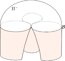
Figure 3. The pants for the triangle

Let us start with a Schottky group of a pair of pants. To introduce this group, let $\alpha$ and $\beta$ be elements of $\mathrm{PSL}(2,\mathbb{R})$ and $A_{\alpha}$, $R_{\alpha}$, $A_{\beta}$, $R_{\beta}$ be disjoint closed intervals in $\mathbb{R}\mathbb{P}^{1}$, such that $\alpha(R_{\alpha}^{c})=\mathrm{Int}(A_{\alpha})$ and $\beta(R_{\beta}^{c})=\mathrm{Int}(A_{\beta})$. The group $\Gamma$ generated by $\alpha$ and $\beta$ is a discrete group. The condition that the quotient $\Gamma\backslash\mathbb{H}^{+}$ is a pair of pants – as opposed to a punctured torus – is that the intervals $A_{\alpha},R_{\alpha},A_{\beta},R_{\beta}$ are in cyclic ordering. Introduce the transformation $\gamma$ in $\mathrm{PSL}(2,\mathbb{R})$ such that $\gamma\beta\alpha=\mathrm{id}$.

Let $q$ be a point in the region delimited by the three axes of $\alpha,\beta,\gamma$ in $\mathbb{H}^{+}$, and $T$ be the triangle $q=\gamma\beta\alpha(q),\alpha(q),\beta\alpha(q)$. The union of the images of $T$ by the elements of $\Gamma$ is a connected part of $\mathbb{H}^{+}$ (see Figure 4). The quotient of the $1$-squeleton of $T$ in $\Gamma\backslash\mathbb{H}^{2}$ is a bouquet of three circles, and the restriction to $T$ of the quotient map $\mathbb{H}^{+}\mapsto\Gamma\backslash\mathbb{H}^{+}$ just consists in identifying the vertices of $T$. We aim to find our branched projective structure on $\Gamma\backslash\mathbb{H}^{-}$ with the image of the interior of $T$ as the negative component, and the branch point of angle $6\pi$ the image of the vertices. To define this structure we will define its developing map $D:\mathbb{H}^{+}\rightarrow\mathbb{C}\mathbb{P}^{1}$, equivariant with respect to the identity.

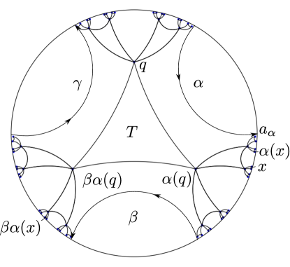
Figure 4. Construction of the triangular real curve

The interior of the triangle $T$ should be negative, and should not contain any branch point, so that the developing map in restriction to $\mathrm{Int}(T)$ needs to be a diffeomorphism from $\mathrm{Int}(T)$ to $\mathbb{H}^{-}$ (by completeness of the hyperbolic metric in the negative component), that extends to a diffeomorphism from $T$ to $\overline{\mathbb{H}^{-}}$. For our purpose, it will be sufficient to consider any diffeomorphism from $T$ to $\overline{\mathbb{H}^{-}}$ such that the points $x=D(q)$, $\alpha(x)$ and $\beta\alpha(x)$ are in cyclic order. We claim that a point $x$ which sits short before the attracting point of $\alpha$ – i.e. the fixed point $a_{\alpha}$ of $\alpha$ lying in $A_{\alpha}$ – is such a point. Indeed, $\alpha(x)$ is between $x$ and , and then $\beta\alpha(x)$ is between $a_{\alpha}$ and the attractive fixed point of $\beta$. i.e. the fixed point of $\beta$ lying in $A_{\beta}$.

Hence we have chosen the diffeomorphism from $T$ to $\overline{\mathbb{H}^{-}}$ as before, we extend $D$ to the union of the images of $T$ by the group $\Gamma$ using the equivariance relation $D(\gamma z)=\gamma D(z)$. The complement of the union of the images of $T$ by the elements of $\Gamma$ is an infinite set of semi-planes. There are three particular ones which are the semi-planes $P_{\alpha}$, $P_{\beta}$ and $P_{\gamma}$ at the left of the piecewise geodesic curves defined respectively by $\cup_{n\in\mathbb{Z}}[\alpha^{n}q,\alpha^{n+1}q]$, $\cup_{n\in\mathbb{Z}}[\beta^{n}\alpha q,\beta^{n+1}\alpha q]$ and $\cup_{n\in\mathbb{Z}}[\gamma^{n}q,\gamma^{n+1}q]$. These curves are mapped by $D$ to the intervals between the repulsive fixed points and the attractive fixed points of $\alpha$, $\beta$ and $\gamma$ respectively. One extends $D$ to a diffeomorphism from $P_{\alpha}$, $P_{\beta}$ and $P_{\gamma}$ to $\mathbb{H}^{+}$ which is equivariant with respect to $\alpha$, $\beta$ and $\gamma$ respectively. All the other components of the complement of $\cup_{\gamma}\gamma T$ is the image of one of the semi-planes $P_{\alpha}$, $P_{\beta}$ or $P_{\gamma}$ by an element of $\Gamma$. Hence, one can extend $D$ to the whole upper half plane $\mathbb{H}^{+}$ by equivariance. This defines a branched projective structure $\sigma_{\Pi}$ on the pair of pants $\Pi=\Gamma\backslash\mathbb{H}^{+}$. By construction it satisfies conditions (1), (2) and (3). We denote by $p$ the branch point of angle $6\pi$ of this structure, and $A_{x}$, $x=\alpha,\beta,\gamma$ the three positive annuli of $\sigma_{\Pi}$ (those are the quotients of $P_{\alpha},P_{\beta}$ ad $P_{\gamma}$ respectively).

To construct an example of a branched projective structure with a ”triangle” peripheral geodesic as described above, we move the branch point $p$ of $\sigma_{\Pi}$ in the positive component.

Figure 5. Moving the $6\pi$-point to the positive part

This movement is done by cutting and pasting $\Pi$ along three curves going from $p$ and entering inside the three positive annuli of $\Pi$ (see Figure 5). We denote these curves by $[p,q_{y}]$, $y=\alpha,\beta,\gamma$, where $q_{y}$ are points in the respective annuli $A_{y}$. After the cut and paste, we get a new structure $(\Pi^{\prime},\sigma_{\Pi^{\prime}})$ on a pair of pants, the three points $q_{y}$’s being identified to a single conical positive point $q$ of angle $6\pi$. We may assume that the segments $(p,q_{y}]\subset\Pi$ are geodesics. Let $\gamma_{y}\subset A_{y}$ be the geodesic loop starting and ending at $q_{y}$ and making a turn around $A_{y}$. Observe that, up to shortening the segments $[p,q_{y}]$, we may assume that the angle between the two branches of $\gamma_{y}$ at $q_{y}$ and $[q_{y},p]$ is approximately $\pi$, and that $\gamma_{y}$ intersects $[q_{y},p)$ only at $q_{y}$. This shows that after the cut and paste, the curves $\gamma_{y}$ produces closed curves $\gamma_{y}^{\prime}$ in $\Pi^{\prime}$ passing through $q$, and that the concatenation $\gamma^{\prime}_{\alpha}*\gamma^{\prime}_{\beta}*\gamma^{\prime}_{\gamma}\subset\Pi^{\prime}$ is the peripheral geodesic associated to the curve $\partial D$. This is due to the fact that the exterior angles of this curve are approximately $2\pi$ at $q$ (see Figure 5).

Then, to get an example on a compact surface, it suffices to glue on the other side of $\Pi^{\prime}$ a pair of pants equipped with a non branched projective structure consisting of a positive component being a pair of pants, and three negative annuli attached to it. We leave the details to the reader.

4. Index formulæ

We provide useful index formulæ à la Goldman (see [7]), for branched projective structures with Fuchsian holonomy relating properties of the previously defined real curve decomposition. Again, these formulas extend to the case where the representation is quasi-Fuchsian, but for simplicity we restrict ourselves to the Fuchsian case.

In this section $S$ is a compact surface equipped with a branched projective structure $\sigma$ with Fuchsian holonomy $\rho$ and developing map $D$. The assumption that no element in the holonomy is elliptic will be of particular importance. Moreover, we suppose that the real curve $S_{\mathbb{R}}$ contains no branch points, so that the components of the real curve are simple closed curves in $S$. Proposition 3.2 and an analytic continuation argument shows that the holonomy of any component of the real curve together with its index (see 3.2) completely determine the projective structure in its neighborhood.

Our aim is to describe numerical relations between the topological invariants of the decomposition, those of the holonomy representation and the indices of the real curves. In particular, inspired by the techniques used by Goldman in [7] for the case of unbranched structures, we provide a useful index formula relating the Euler invariant of $\rho$, the Euler characteristic of the components of $S^{\pm}$, the number of their branch points and the indices of their boundaries (see Theorem 4.1 below).

Next we will focus on the topological properties of the representation $\rho$. Recall that given an oriented closed surface with boundary $C$ and a Fuchsian representation $\rho:\pi_{1}(C)\rightarrow{\rm PSL}(2,\mathbb{R})$ we can naturally associate a $\mathbb{RP}^{1}$-bundle $F_{\rho}\rightarrow C$ equipped with a flat connection. Indeed, $F_{\rho}$ is obtained as the quotient of $\widetilde{C}\times\mathbb{RP}^{1}$ by the action of $\pi_{1}(C)$ such that for $\gamma\in\pi_{1}(C)$ and $(p,z)\in\widetilde{C}\times\mathbb{RP}^{1}$

(2) $$\gamma\cdot(p,z)=(\gamma(p),\rho(\gamma)(z)).$$

If the boundary is empty, we can define the Euler number of $\rho$ as the element $eu(\rho)=eu(F_{\rho})\in H^{2}(C,\mathbb{Z})=\mathbb{Z}$ defined by the Euler class of the bundle $F_{\rho}$. Otherwise, if there are no elliptic elements, over each component $l\subset\partial C$ we can define a section of $s_{\rho}:l\rightarrow(F_{\rho})|_{l}$ by following a fixed point of the action of $\rho(l)$ on $\mathbb{RP}^{1}$ along $l$ with the use of the connection. If $\rho(l)$ is the identity or loxodromic, the homotopy class of the section is independent of the chosen fixed point. As we will show shortly we can associate an Euler number $eu(\rho)\in\mathbb{Z}$ to the representation by using the pair $(F_{\rho},s_{\rho})$. In the sequel we will prove the following

Theorem 4.1 (First Index Formula).

Let $S$ be a compact surface equipped with a BPS $\sigma$ with Fuchsian holonomy. Suppose no branch point belongs to $S_{\mathbb{R}}$. Let $C$ be a component of $S\setminus S_{\mathbb{R}}$ with the orientation induced by that of $S$ and denote by $\rho_{C}$ the restriction of $\rho$ to $\pi_{1}(C)$.

If $k$ denotes the number of branch points in $C$ and $l_{1},\ldots l_{n}$ are the components of $\partial C\subset S_{\mathbb{R}}$, then

$$\pm eu(\rho_{C})=\chi(C)+k-\sum_{i=1}^{n}I_{l_{i}}$$

where the sign is positive if $C\subset S^{+}$ and negative otherwise.

Corollary 4.2 (Second Index Formula).

If there are no branch points on the real curve and $k^{\pm}$ denotes the number of branch points contained in $S^{\pm}$ then

$$eu(\rho)=(\chi(S^{+})+k^{+})-(\chi(S^{-})+k^{-}).$$

For the proof of the theorem it will be convenient to have the theory of Euler classes of sections of oriented circle bundles at hand.

Let $F\rightarrow C$ be an oriented $\mathbb{RP}^{1}$-bundle over a compact oriented surface with boundary $C$. For each section $s:\partial C\rightarrow\mathbb{RP}^{1}$ we define the Euler number $eu(F,s)$ as follows. Consider a triangulation $\tau$ of $C$ such that over each triangle $T$ of $\tau$ the bundle is isomorphic to $T\times\mathbb{RP}^{1}$. By connectedness of $\mathbb{RP}^{1}$ the section $s$ can be extended continuously to a section $\overline{s}$ defined on the 1-skeleton of $\tau$. The restriction of $\overline{s}$ to $\partial T$ can be thought of as a map $s:\partial T\rightarrow\mathbb{RP}^{1}$ that has degree $n_{T}\in\mathbb{Z}$ with respect to the given orientations. The sum $\sum n_{T}$ can be shown to be independent of the triangulation and the chosen extension $\overline{s}$ through basic algebraic topology methods. This allows to define

$$eu(F,s)=\sum n_{T}.$$

In fact $eu(F,s)$ depends only on the homotopy class of $s$.

Remark 4.3.

If $C=\mathbb{S}^{1}\times[0,1]$ is an annulus and $s=\{s_{i}\}$ is a section of $F$ over $\mathbb{S}^{1}\times\{i\}$ for $i=0,1$ then $eu(F,s)=\deg f$ where $f:\mathbb{S}^{1}\rightarrow\mathbb{RP}^{1}=\mathbb{S}^{1}$ is such that $s_{0}=f\cdot s_{1}$ and the degree is computed with respect to the orientation induced by $C$ on the component where $s_{0}$ is defined.

The following lemma is immediate.

Lemma 4.4.

Let $F$ be an oriented $\mathbb{RP}^{1}$-bundle over $\overline{C}$ and $\{\lambda_{i}\}$ be a finite family of disjoint simple closed curves in $\overline{C}$ containing the boundary components of $C$. Let $s$ be a continuous section of $F$ defined on $\cup_{i}\lambda_{i}$. Denote by $\{C_{j}\}_{j}$ the collection of the closure of connected components of $C\setminus\big{(}\cup_{i}\lambda_{i}\big{)}$. Then

$$eu(F,s|_{\partial C})=\sum_{j}eu(F|_{C_{j}},s|_{\partial C_{j}}).$$

To abridge notations, rename $\rho_{C}$ as $\rho$. We define

$$eu(\rho):=eu(F_{\rho},s_{\rho})$$

where the pair $(F_{\rho},s_{\rho})$ was defined by the relations in (2), shortly before the statement of Theorem 4.1.

Remark 4.5.

If $S$ is a compact surface and $\rho:\pi_{1}(S)\rightarrow\mathrm{PSL}(2,\mathbb{C})$ is a Fuchsian representation, by using the uniformizing structure on $S$ it is easy to show that for any incompressible subsurface $C\subset S$ we have

$$eu(\rho|_{\pi_{1}(C)})=\chi(C).$$

Let us proceed to the proof of Theorem 4.1. Given the connected component $C$ of $S\setminus S_{\mathbb{R}}$, we introduce $E=\mathbb{P}^{+}(TC)$ the $\mathbb{RP}^{1}$-bundle over $C$ whose fibre over $p\in C$ is the set of semi-lines in $T_{p}C$. For each branch point $p\in C$ we consider a small open disc $B$ in $C$ centered at $p$. We number such discs $B_{1},\dots,B_{k}$ and call $\lambda_{i}$ their boundary curves. On the other hand, for each boundary component $l_{i}$ of $\partial C$ consider a curve $\bar{l}_{i}$ in $C$ that is isotopically equivalent to $l_{i}$ in $\overline{C}\setminus\cup_{j}B_{j}$. The proof of Theorem 4.1 consists in using the developing map $D$ to define a bundle isomorphism $\mathrm{D}:E\rightarrow F_{\rho}$ over $C\setminus\cup_{j}B_{j}$ , which allows to define a section of $F_{\rho}$ over the family of curves $\{\bar{l}_{1},\ldots,\bar{l}_{n},\lambda_{1},\ldots,\lambda_{k}\}$ and apply Lemma 4.4. The conclusion will follow from the knowledge on the topology of the associated decomposition and the properties of $D$.

Consider a lift $\widetilde{C^{*}}\subset\widetilde{S}$ of $C^{*}:=C\setminus\{\textrm{branch points}\}$. The restriction of the developing map $D$ to $\widetilde{C^{*}}$ or its complex conjugate defines a local diffeomorphism $\mathbf{D}:\widetilde{C^{*}}\rightarrow\mathbb{H}^{2}$ that preserves orientation if $C$ is positive and reverses it otherwise. In either case $\mathbf{D}$ induces a map

$$\mathbb{P}^{+}(T\widetilde{C^{*}})\rightarrow\widetilde{C^{*}}\times\mathbb{P}^{+}(T\mathbb{H}^{2})$$

defined by $(p,[v_{p}])\mapsto(p,[d\mathbf{D}_{p}(v_{p})])$, where the brackets denote equivalence classes under multiplication by a positive real number. Recall that the complete hyperbolic metric on $\mathbb{H}^{2}$ induces a map $\infty:P^{+}(T\mathbb{H}^{2})\rightarrow\mathbb{RP}^{1}$ that is equivariant under the natural actions of ${\rm PSL}(2,\mathbb{R})$ on source and target. Indeed, for each point $(p,[v_{p}])\in P^{+}(T\mathbb{H}^{2})$ we associate the point $\infty(p,[v_{p}])\in\partial\mathbb{H}^{2}=\mathbb{RP}^{1}$ obtained by following the unique geodesic passing through $p$ tangent to $v_{p}$ until infinity in the direction of $v_{p}$. This allows to consider the map

$$\mathbb{P}^{+}(T\widetilde{C^{*}})\rightarrow\widetilde{C^{*}}\times\mathbb{RP}^{1}$$

defined by $(p,[v_{p}])\mapsto(p,\infty(p,[d\mathbf{D}_{p}(v_{p})]))$ which is equivariant with respect to the actions of $\pi_{1}(C)$ on $\mathbb{P}^{+}(T\widetilde{C^{*}})$ by deck transformations and on $\widetilde{C^{*}}\times\mathbb{RP}^{1}$ by $id\times\rho$. Hence it induces an isomorphism of $\mathbb{RP}^{1}$-bundles over $C^{*}$

$$\mathrm{D}:\mathbb{P}^{+}(TC^{*})=E|_{C^{*}}\rightarrow(F_{\rho})|_{C^{*}}.$$

Next we define a section $t$ of $F_{\rho}$ over the family of curves

$$L=\{l_{1},\ldots,l_{n},\bar{l_{1}},\ldots,\bar{l_{n}},\lambda_{1},\ldots,\lambda_{k}\}.$$

Over each of the boundary components $l_{i}$, $t$ is the section defined by a fixed point of $\rho(l_{i})$; over any other component $c$, $t$ is the image by $\mathrm{D}$ of the section $p\mapsto(p,c^{\prime}(p))$ of $E$ where the orientation of the parametrization is that of $l_{i}$ if $c=\bar{l_{i}}$ and that of $\partial B_{i}$ if $c=\lambda_{i}$. The complement of $L$ in $\overline{C}$ is a disjoint union of annuli $A_{1},\ldots,A_{n}$ each having exactly one boundary component in $\partial C$, discs $B_{1},\ldots,B_{R}$ and a component $C^{\prime}\subset C$. By Lemma 4.4

$$eu(\rho)=eu(F_{\rho},t)$$

$$= eu\big{(}(F_{\rho})|_{C^{\prime}},t|_{\partial C^{\prime}}\big{)}+\sum_{j=1}^{R}eu\big{(}(F_{\rho})|_{B_{j}},t|_{\partial B_{j}}\big{)}+\sum_{i=1}^{n}eu\big{(}(F_{\rho})|_{A_{i}},t|_{\partial A_{i}}\big{)}.$$

Now, since $\mathbf{D}$ is a local diffeomorphism when restricted to a lift $\widetilde{C^{\prime}}\subset\widetilde{C}$ of $C^{\prime}$, $\mathrm{D}|_{C^{\prime}}$ is a bundle isomorphism $E|_{C^{\prime}}\rightarrow(F_{\rho})|_{C^{\prime}}$ and hence

$$eu\big{(}(F_{\rho})|_{C^{\prime}},t|_{\partial C^{\prime}}\big{)}=\pm\chi(C^{\prime})$$

where the sign is positive if $\mathbf{D}$ preserves orientation and negative otherwise. On the other hand since $\mathbf{D}$ has a single simple branch point on the disc $B_{j}$,

$$eu\big{(}(F_{\rho})|_{B_{j}},t|_{\partial B_{j}}\big{)}=\deg(t|_{\partial B_{j}})=\pm 2$$

where the sign is positive if $\mathbf{D}$ preserves orientation and negative otherwise. Finally for an annulus $A_{i}$ denote by $\phi:l_{i}\rightarrow\bar{l}_{i}$ the homeomorphism induced by the isotopy joining $l_{i}$ with $\bar{l}_{i}$. As noted in Remark 4.3, if we write $t|_{l_{i}}=f\cdot(t|_{\bar{l}_{i}}\circ\phi)$, then by the definition of the index of $l_{i}$

$$eu\big{(}(F|_{\rho})_{A_{i}},t|_{\partial A_{i}}\big{)}=\deg f=\mp I_{l}.$$

Since $\deg f$ is measured with respect to the orientation induced on $l_{i}$ by that of $C$ , the sign is negative if $\mathbf{D}$ preserves orientation and positive otherwise. By summing up we get

$$eu(\rho)=\pm\big{(}\chi(C^{\prime})+2k-\sum_{i=1}^{n}I_{l_{i}}\big{)}=\pm\big{(}\chi(C)+k-\sum_{i=1}^{n}I_{l_{i}}\big{)}$$

where the sign is positive if if $\mathbf{D}$ preserves orientation and negative otherwise. This finishes the proof of Theorem 4.1.

For the proof of Corollary 4.2, by considering over each $l_{i}$ the section of $F_{\rho}$ associated to a fixed point of $\rho(l_{i})$, and applying Lemma 4.4, we have

$$eu(\rho)=eu(\rho^{+})+eu(\rho^{-})$$

where $eu(\rho^{\pm})$ denotes the Euler number of $\rho$ restricted to $\pi_{1}(S^{\pm})$. An instance of Theorem 4.1 on each connected component of $S^{\pm}$ and the fact that each curve $l_{i}$ is the boundary of exactly one positive and one negative component give

$$eu(\rho) = \big{(}\chi(S^{+})+k^{+}-\sum_{i=1}^{n}I_{l_{i}}\big{)}-\big{(}\chi(S^{-})+k^{-}-\sum_{i=1}^{n}I_{l_{i}}\big{)}$$

$$= \big{(}\chi(S^{+})+k^{+}\big{)}-\big{(}\chi(S^{-})+k^{-}\big{)}.$$

As another application of Theorem 4.1, we note that if $\chi(S)\leq 0$, one has $\chi(S)=eu(\rho)$ because $\rho$ is Fuchsian. From $\chi(S)=\chi(S^{+})+\chi(S^{-})$ we therefore obtain

$$2\chi(S^{-})=k^{+}-k^{-}.$$

Corollary 4.6.

If $A$ is an annulus with loxodromic holonomy $\rho$ then $eu(\rho)=0$.

5. Grafting and bubbling

In this section we will prove that grafting can be obtained by a bubbling followed by a debubbling, as was stated in Theorem  1.2 in the Introduction. We recall that a graftable curve is a simple closed curve with loxodromic holonomy such that the developing map is injective on one of its lifts. A more precise restatement of Theorem 1.2 is:

Theorem 5.1.

Let $\sigma$ be a BPS on a surface $S$ and $\gamma$ be a graftable simple closed curve in $S$ that does not pass through the branch points of $\sigma$. Then the grafting of $\sigma$ along $\gamma$ can be obtained by a bubbling followed by a debubbling on $\sigma$.

Proof.

First, remark that a small annular neighborhood $U$ of $\gamma$ has a lift in the universal cover that develops injectively in $\mathbb{CP}^{1}$. Everything will take place in that annular neighborhood. The whole process of bubbling and debubbling is sketched in Figure 6, and details are described below.

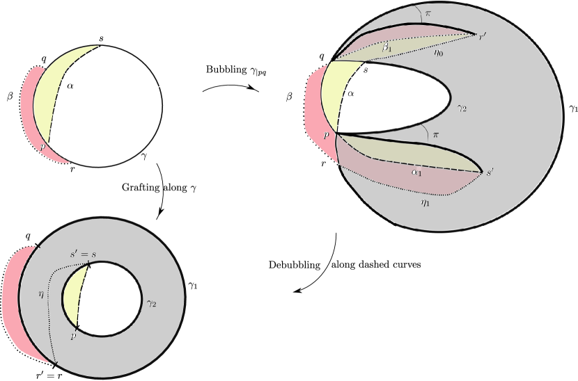
Figure 6. Grafting can be obtained by bubbling and debubbling

We choose an orientation for $\gamma$. Consider four points $s,q,p,r\in\gamma$ in cyclic order. Choose paths $\alpha$ and $\beta$ joining $s$ to $p$ and $q$ to $r$, obtained by pushing the segments $[s,p]$ and $[q,r]$ on the left and on the right side of $\gamma$ respectively, as in the upper left corner of Figure 6. We denote by $\widetilde{\gamma}$ a lift of $\gamma$ to the universal cover of $S$, $\widetilde{U}$ the corresponding lift of $U$, by $D$ the developing map of $\sigma$ and by $\rho$ the (loxodromic) holonomy of $\gamma$. Consider one of the images $p_{0},q_{0},r_{0},s_{0},\alpha_{0},\beta_{0}\subset\mathbb{CP}^{1}$ by $D$ of each of the corresponding elements in the initial situation and call $p_{1},q_{1},r_{1},s_{1},\alpha_{1},\beta_{1}\subset\mathbb{CP}^{1}$ the images of the latter by $\rho$ (see Figure 7).

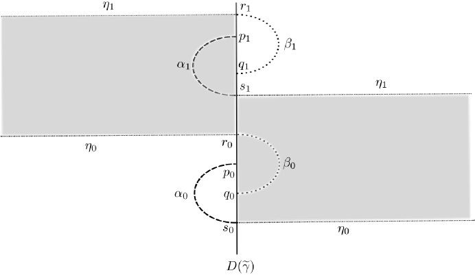
Figure 7. Developed image in $\mathbb{CP}^{1}$

Consider the annulus $A=(\mathbb{CP}^{1}\setminus\overline{D(\widetilde{\gamma})})/<\rho>$ equipped with its natural projective structure. Still denote by $\alpha$ and $\beta$ of the image in $A$ of the $\alpha_{i}$’s and $\beta_{i}$’s. We denote by $s,q,p,r$ their respective extremities in $\partial A$ (therefore $q,r$ lie in a component of $\partial A$ and $p,s$ on the other one). In particular we can find a simple arc $\eta$ in $A$ joining the points $r$ to $s$ and avoiding the developed images of $\alpha$ and $\beta$. In Figure 7 we find a sketch of two lifts $\eta_{0}$ and $\eta_{1}$ of $\eta$ to $\mathbb{CP}^{1}$. They will be important for the construction of twin paths.

Next we consider the bubbling $\mathrm{bub}(\sigma)$ of $\sigma$ along the oriented arc $[p,q]$ of $\gamma$ between $p$ and $q$ (the one that contains the points $r$ and $s$), see Figure 6, right side. This is obtained by cutting $\sigma$ along $[p,q]$ and $\mathbb{CP}^{1}$ along $[p_{0},q_{1}]$ (see Figure 7) and pasting together. Two branch points of angle $4\pi$ appear at $p$ and $q$. The oriented segment $[p,q]$ in $\sigma$ is separated into twins segments $[p,q]_{\rm right}$ and $[p,q]_{\rm left}$ in $\mathrm{bub}(\sigma)$. Observe that the arcs $\alpha$ and $\beta$ in $S$ survive after the bubbling. We denote their endpoints in $\mathrm{bub}(\sigma)$ with the same letters, $s,p,q,r$ as before the bubbling ($r$ lives in $[p,q]_{\rm right}$ and $s$ lives in $[p,q]_{\rm left}$).

We proceed now to see that there is another bubble in $\mathrm{bub}(\sigma)$, such that its debubbling is the grafting $\textrm{Gr}_{\gamma}(\sigma)$ of $\sigma$ along $\gamma$. To identify a bubble it is sufficient to find a pair of twin paths that join two simple branch points, bound a disc, and develop to a segment. Consider the paths in $\mathrm{bub}(\sigma)$ starting at $q$,

$$\tau_{1}=\beta\star\eta_{0}\star\alpha_{0}\ \ \ \text{and}\ \ \ \tau_{2}=\beta_{1}\star\eta_{1}\star\alpha,$$

that are drawn with dashed lines on the right part of Figure 6. These paths are twins. Moreover, we claim that $\tau_{1}*\tau_{2}^{-1}$ bounds a disc. Indeed, the curve $[p_{0},r_{0}]\star\eta_{0}\star\alpha_{0}$ in $\mathbb{CP}^{1}\setminus[p_{0},q_{1}]$ bounds a disc $\mathrm{Disc}_{0}$, and similarly $\beta_{1}\star\eta_{1}\star[s_{1},q_{1}]$ bounds a disc $\mathrm{Disc}_{1}$. Clearly $\beta\star[p,r]^{-1}\star\alpha^{-1}\star[s,q]$ bounds a disc in $\sigma$. These three discs glue together to a disc bounded by $\tau_{1}*\tau_{2}^{-1}$.

We are left to prove that the debubbling of these twin paths produces a new branched projective structure that coincides with $\textrm{Gr}_{\gamma}(\sigma)$. To this end, it suffices to find two parallel curves whose developed image is precisely $D(\widetilde{\gamma})$, bounding an annulus with the projective structure of $A$, and whose complement has the structure induced by $\sigma$ on $S\setminus\gamma$.

We proceed to analyze the preimages of $D(\widetilde{\gamma})$ via the developing map of $\mathrm{bub}(\sigma)$ to identify such curves. Denote by $\gamma_{1}$ the segment $[r,q]\subset[p,q]_{\mathrm{right}}$ and $\gamma_{2}$ the segment $[p,s]\subset[p,q]_{\mathrm{left}}$. as in Figure 6. Remark that the twin path of the segment $[s,p]$ in $\gamma$ starting from $p$ is the segment $[p,s_{0}]$ (in the bubble $\mathbb{CP}^{1}\setminus[p_{0},q_{1}]$) that joins $p=p_{0}$ and $s_{0}$ and that does not enter the second bubble till $s_{0}$, as $\mathrm{Disc}_{0}$ is delimited by $\alpha_{0}$, see Figure 7. Similarly, the twin path $[q,r_{1}]$ of the segment $[q,r]$ joins $q$ and $r_{1}$ in the first bubble without entering the second bubble. These twins correspond to the thick segments inside the shaded bubble in Figure 6). Thus they appear in the structure after the debubbling and will have developed image contained in $D(\widetilde{\gamma})$. By construction, after the debubbling their union with $\gamma_{1}$ and $\gamma_{2}$ form a pair of parallel closed curves having the same developed image.

The shaded part in Figure 7 is, by construction, a fundamental domain for the action of $\rho$ on $\mathbb{CP}^{1}\setminus\textrm{Fix}(\rho)$. Moreover, the region bounded by $\alpha_{0}\star[p,s_{0}]$ is projectively equivalent to the region delimited by $\alpha\star[s,p]^{-1}$. Similarly, the region bounded by $\beta\star[r_{1},q]$ is projectively equivalent to the one delimited by $\beta\star[q,r]^{-1}$. This implies both properties we need: namely that the projective structure in the region between $\tau_{1}$ and $\tau_{2}$ after debubbling coincides with $A$, and that the structure on the complement of $A$ is the one induced by $\sigma$ on $S\setminus\gamma$. ∎

6. Finding embedded twin paths

In this section, we give two criteria to ensure that a pair of twin paths is embedded. This is necessary to perform all the movements of branch points we carry in Sections 7, 8, and 9.

The pathologies that one has to avoid are mainly two. Suppose that we have a geodesic ray $\tau$ emanating from a branch point and want to follow its twin $\tau^{\prime}$, which is locally well-defined. Even if $\tau$ is embedded it could happen that $\tau^{\prime}$ is wild (remark that a bubbling introduces a whole copy of the universal cover of the surface!). Secondly, it could happen that $\tau^{\prime}$ crosses $\tau$ very soon, say $\tau(\varepsilon)=\tau^{\prime}(\varepsilon)$ at a smooth point (as in fact happens in a conical cut and paste described at page 2.2) with no a priori control on $\varepsilon$. In both cases a cut and paste procedure would change the topology of $S$.

Here we prove two lemmas. The first one ensures that if we follow the pre-image of a geodesic under a projective map, the twin paths we obtain are in fact embedded. The second shows that if the holonomy is Fuchsian, then pathologies like the conical cut and paste cannot occur. Both lemmas rely on the hypothesis of Fuchsian holonomy and their falseness in more general settings constitutes one of the main obstructions to generalize the arguments to other types of representations.

Lemma 6.1 (Twin geodesics are embedded).

Suppose $S$ is a surface equipped with a BPS having Fuchsian holonomy. Let $U\subset S^{\pm}$ be an open domain in $S^{\pm}$ with smooth boundary and corners. Let $\Sigma$ be a complete hyperbolic surface, and $f:U\rightarrow\Sigma$ be a local isometry (on the complement of branch points). Let $T\in[0,\infty]$ and $(\tau_{1},\tau_{2})$ be a pair of twin geodesics $\tau_{i}:[0,T)\rightarrow U$ starting at a branch point $p\in\overline{U}$ such that

• for every $i=1,2$ and $t\in(0,T)$, $\tau_{i}(t)$ belongs to $U$ and is not a branch point of $S$,

• $f\circ\tau_{1}=f\circ\tau_{2}=\tau$ is a properly embedded geodesic in $\Sigma$.

Then, $(\tau_{1},\tau_{2})$ is a pair of embedded twin paths in $S$. Moreover, suppose that $\Sigma$ does not have parabolic ends and that $T=+\infty$. Then $\tau_{i}(t)$ tends to a point $u_{i}$ in $S_{\mathbb{R}}$ when $t$ tends to infinity, for $i=1,2$, with $u_{1}\neq u_{2}$.

Proof.

Each of the paths $\tau_{i}$’s are embedded since $\tau$ is embedded. The first part of the lemma says that the images of $\tau_{1}$ and $\tau_{2}$ are disjoint. We argue by contradiction. Suppose that there are two numbers $0\leq s,t<T$, not both equal to $0$, such that $\tau_{1}(s)=\tau_{2}(t)$. Because $\tau$ passes once through the point $p$, both $s$ and $t$ are positive. By exchanging the roles of $\tau_{1}$ and $\tau_{2}$ if necessary, we can suppose that $s\geq t$.

At the point $q=\tau_{1}(s)=\tau_{2}(t)$, the geodesics $\tau_{1}$ and $\tau_{2}$ cannot be transverse, because the map $f$ is a local diffeomorphism at $q$. Hence, we necessarily have $\tau_{1}(s+u)=\tau_{2}(t+u)$ for small values of $u$, or $\tau_{1}(s-u)=\tau_{2}(t+u)$ for small values of $u$. In the first case, we have $\tau_{1}(s+u)=\tau_{2}(t+u)$ for every $u\geq-t$ by analytic continuation. Because $\tau_{1}$ and $\tau_{2}$ are different, we have $s>t$. At $u=-t$, we find $\tau_{1}(s-t)=\tau_{2}(0)=p$. Hence $\tau(s-t)=p$ which contradicts that $\tau$ is embedded. In the second case, we get $\tau_{1}(s-u)=\tau_{2}(t+u)$ for $0\leq u\leq(s-t)/2$ by analytic continuation (note that $t+(s-t)/2\leq s<T$). In particular we get $\tau_{1}(\frac{s+t}{2})=\tau_{2}(\frac{s+t}{2})$. At $u=(s+t)/2>0$, we therefore obtain that $f$ is a branched covering, contradicting the hypothesis that $\tau_{1}(t)$ is not a branch point of $S$ for $t>0$. The first claim is proved.

Since $\tau$ is properly embedded both $\tau_{1}$ and $\tau_{2}$ must exit any compact set of $S$ as $t\to\infty$, otherwise an accumulation point would exists. By Lemma 3.5 both $\tau_{i}$’s have limits $u_{i}$ as $t\to\infty$. Such limits must belong to $S_{\mathbb{R}}$ because both $\tau_{i}$ exist all compact.

If $u_{1}=u_{2}$, then $\tau_{1}$ and $\tau_{2}$ are exponentially asymptotic at infinity in $U$ for the hyperbolic distance. However, they have the same image $\tau$ by $f$, and $\Sigma$ has no parabolic end, so this is impossible. Hence the limits are distinct, and the lemma is proved. ∎

Suppose that the holonomy of $S$ is Fuchsian. For a component $C\subset S^{\pm}$ we denote by $C_{fuchs}$ the hyperbolic surface $\rho(\pi_{1}(C))\backslash\mathbb{H}^{\pm}$. The following lemma shows that we can always move branch points at least a distance bounded below by the injectivity radius of $C_{fuchs}$.

Lemma 6.2 (Local movements).

Let $S$ be a closed surface equipped with a BPS with Fuchsian holonomy. Let $C$ be a component of $S^{\pm}$ and let $\varepsilon>0$ be smaller than the injectivity radius of $C_{fuchs}$. Let $\gamma$ be a geodesic segment starting from a branch point $p$ of $C$ and shorter than $\varepsilon$. Let $\gamma^{\prime}$ be a geodesic segment starting from $p$, of the same length as $\gamma$, and forming with $\gamma$ at $p$ an angle $2k\pi$, with $0<k\in\mathbb{N}$. Suppose that both $\gamma$ and $\gamma^{\prime}$ do not contain branch points other than $p$. Then $\gamma$ and $\gamma^{\prime}$ form a pair of embedded twin paths.

Proof.

A developing map for $S$ induces a map $f:C\to C_{fuchs}$ which is a local isometry. The image of $\gamma$ is therefore a geodesic in $C_{fuchs}$. Since $\gamma$ is shorter than the injectivity radius of $C_{fuchs}$, then $f(\gamma)$ is properly embedded. As $\gamma^{\prime}$ forms an angle $2k\pi$, we have $f(\gamma)=f(\gamma^{\prime})$ and Lemma 6.1 concludes. ∎

7. Debubbling adjacent components

In this section, we give a criterion ensuring that a BPS can be debubbled, after possibly moving the branch points. The main result is the following.

Theorem 7.1 (Debubbling).

Let $S$ be a compact surface equipped with a BPS $\sigma$ having Fuchsian holonomy. Suppose that there exists a positive and a negative component, that we denote $C^{+}$ and $C^{-}$, with a common boundary component $l$, such that

1. the index of $l$ is $1$, and its holonomy is loxodromic,

2. the index of any component of $\partial C^{+}$ or $\partial C^{-}$ other than $l$ vanishes,

3. each component $C^{+}$ and $C^{-}$ contains a single branch point of angle $4\pi$.

Then, after possibly moving the branch points in the components $C^{+}$ and $C^{-}$, the branched projective structure on $C^{+}\cup C^{-}$ is a bubbling.

Before entering into the details, let us explain the strategy for the proof of this result, and introduce the notion of half-bubble:

Definition 7.2 (Half-bubble).

Given a positive or negative component $C$ of $\sigma$ and a component $l$ of $\partial C$, a half-bubble in the direction of $l$ is a pair of embedded twin geodesics $(\tau_{1},\tau_{2})$ contained in $C$ and tending at different points $u_{1}$ and $u_{2}$ of $l$ at infinity, such that $C\setminus(\tau_{1}\cup\tau_{2})$ has two connected components, one of them being isometric via the developing map to $\mathbb{H}^{2}$ minus a semi-infinite geodesic. We require moreover that the oriented angle $\measuredangle\tau_{1}\tau_{2}$ is the $2\pi$-angle of that region.

In other words, the branched $\mathbb{H}^{2}$-structure on $C$ has been obtained from another branched $\mathbb{H}^{2}$-structure $C^{\prime}$ by inserting a hyperbolic plane with a cut and paste procedure along a properly embedded semi-infinite geodesic of $C^{\prime}$.

The proof of Theorem 7.1 consists in finding half-bubbles in the direction of $l$ in each of the components $C^{+}$ and $C^{-}$ and ensure that, after possibly moving the branch points in $C^{+}$ and $C^{-}$, they glue together to produce a bubble. This is done in Proposition 7.8.

Recall that a connected subsurface $C\subset S$ is called incompressible if any loop in $C$, which is homotopically trivial in $S$, is also homotopically trivial in $C$.

Lemma 7.3.

The components $C^{+}$ and $C^{-}$ are incompressible in $S$.

Proof.

A well-known criterion for a connected subsurface of $S$ to be incompressible is that its boundary components are not homotopically trival in $S$. By hypothesis $l$ has loxodromic holonomy. Since any component $l^{\prime}$ of $\partial C^{+}$ or $\partial C^{-}$ different from $l$ has index $0$, its holonomy is non-trivial (see Proposition 3.2.) Thus, neither $l$ nor any $l^{\prime}$ can be homotopically trivial. ∎

Remark that Lemma 7.3, Remark 4.5 and the index formula 4.1 show that necessarily $C^{-}$ is an annulus. However, $C^{+}$ may have more complicated topology.

It is necessary now to fix some notation. Let $\rho$ denote the holonomy of a developing map $D$ for $\sigma$. The facts we are going to prove hold true for both $C^{+}$ and $C^{-}$. For lightening notations we fix $C=C^{+}$. In order to obtain the proofs for $C^{-}$ one has just to replace the upper half-plane model for $\mathbb{H}^{2}$ with the lower half-plane model for $\mathbb{H}^{-}$.

Let $\pi:\widetilde{S}\rightarrow S$ be the universal covering of $S$, with covering group $\pi_{1}(S)$. We chose a connected component $\widehat{C}$ of $\pi^{-1}(C)$. The restriction of $\pi$ to $\widehat{C}$ is a Galois covering over $C$, with Galois group the stabilizer of $\widehat{C}$ in $\pi_{1}(S)$. We set $\pi_{1}(C)=\operatorname{Stab}(\widehat{C})<\pi_{1}(S)$ (note that using this notation, in general the group $\pi_{1}(C)$ could be different from the fundamental group of $C$, for instance if $C$ were compressible in $S$). As above, we denote by $C_{fuchs}$ the complete hyperbolic surface

$$C_{fuchs}:=\rho(\pi_{1}(C))\backslash\mathbb{H}^{2}.$$

The restriction of $D$ to $\widehat{C}$, induces a map $D_{C}:C\rightarrow C_{fuchs}$, which is a local isometry.

The topology of $C_{fuchs}$ may be very different from that of $C$. For instance, for a BPS with discrete holonomy in $PSL(2,\mathbb{R})$, a positive component $C$ may be diffeomorphic to a pair of pants but $C_{fuchs}$ to a disc (case of a branched covering over $\mathbb{C}\mathbb{P}^{1}$) or to a punctured torus.

Example 7.4.

Consider a complete hyperbolic metric on a punctured torus $\Sigma$, with a cusp of infinite area. Let $\gamma\subset\Sigma$ be a properly embedded semi-infinite geodesic. Let $\alpha$ and $\beta$ be some generators of the fundamental group of $\Sigma$, and let

$$\pi_{\alpha}:\Sigma_{\alpha}=\widetilde{\Sigma}/\alpha\rightarrow\Sigma,\ \ \ \ \ \pi_{\beta}:\Sigma_{\beta}=\widetilde{\Sigma}/\beta\rightarrow\Sigma$$

be the intermediate coverings defined by $\alpha$ and $\beta$; both are isometric to loxodromic annuli. Let $\gamma_{\alpha}$ and $\gamma_{\beta}$ be some lifts of $\gamma$ by $\pi_{\alpha}$ and $\pi_{\beta}$. These semi-infinite paths are properly embedded as well. Let us cut $\Sigma_{\alpha}$ and $\Sigma_{\beta}$ and paste these annuli along these cuts. One obtains a pair of pants $\Pi$ together with a hyperbolic metric with one conical point of angle $4\pi$. Moreover, the maps $\pi_{\alpha}$ and $\pi_{\beta}$ glue together to produce a map $D:\Pi\rightarrow\Sigma$, which is a local isometry and a $\pi_{1}$-isomorphism (see [31, Lemma 4, p. 658] for more details).

However, such examples are incompatible with our Fuchsian assumption:

Lemma 7.5 (Identification between $C$ and $C_{fuchs}$).

Let $S$ be a closed surface equipped with a BPS with Fuchsian holonomy. If $C$ is an incompressible component of $S^{\pm}$, then there is an orientation preserving diffeomorphism $\Phi:C_{fuchs}\rightarrow C$ such that the map induced by $D_{C}\circ\Phi$ on the set of free-homotopy classes of closed loops is the identity.

Proof.

Since $C$ is incompressible, any connected component of $\pi^{-1}(C)$ is simply connected. If follows that $\widehat{C}$ is the universal covering of $C$ and the Galois group $\pi_{1}(C)$ is indeed isomorphic to the fundamental group of $C$, via an isomorphism that is well-defined up to conjugation.

It is classical to see that there exists an orientation preserving diffeomorphism $\widetilde{F}:\widetilde{S}\to\widehat{C}$ that is $\pi_{1}(C)$-equivariant and $\pi_{1}(C)$-equivariantly homotopic to the identity. On the other hand, since $\rho$ is Fuchsian and $S$ is closed, there is a $\rho$-equivariant orientation preserving diffeomorphism $\widetilde{G}:\widetilde{S}\to\mathbb{H}^{2}$. The map $\widetilde{\Phi}=\widetilde{F}\circ\widetilde{G}^{-1}$ descends to a diffeomorphism $\Phi:C_{fuchs}\to C$. Since $D$ is $\rho$-equivariant, the map $D\circ\widetilde{\Phi}$ has the property that

$$D(\widetilde{\Phi}(h\cdot x))=h\cdot D(\widetilde{\Phi}(x))$$

for all $h\in\rho(\pi_{1}(C))$. Since $\rho(\pi_{1}(C))$ is the Galois group of the universal covering $\mathbb{H}^{2}\to C_{fuchs}$, it follows that $D\circ\Phi$ fixes free-homotopy classes of loops.

∎

We identify $C$ with $C_{fuchs}$ using the diffeomorphism $\Phi$ of Lemma 7.5 so that now it makes sense to say that $D_{C}$ fixes free homotopy classes of loops. We still use the notation $C$ and $C_{fuchs}$ to mean that the structure of $C$ is the branched one while that of $C_{fuchs}$ is the hyperbolic unbranched one.

Since the holonomy of $l$ is loxodromic, we consider the geodesic representatives $\gamma$ in $C$ and $\gamma_{fuchs}$ in $C_{fuchs}$ in the respective homotopy classes. Note that $D_{C}(\gamma)$ is in general different from $\gamma_{fuchs}$ (they only belong to the same homotopy-class), since $D_{C}$ is not a global isometry. As above, we denote by $E_{l}$ the end of $C$ corresponding to $l$. If $C_{fuchs}$ is an annulus let $E_{fuchs}$ be the end which is on the same side of $\gamma_{fuchs}$ as $E_{l}$ of $\gamma$. Otherwise $E_{fuchs}$ is just the end of $C_{fuchs}$ corresponding to $l$. In both cases $E_{fuchs}$ is an annulus with geodesic boundary $\gamma_{fuchs}$ and a complete hyperbolic metric with loxodromic holonomy.

In order to prove Theorem 7.1, we begin by moving the branch point $p$ in $C$ so that its image $q=D_{C}(p)$ in $C_{fuchs}$ belongs to $\gamma_{fuchs}$. To this end, let $\delta$ be an embedded geodesic segment starting at $q$ and ending at a point of $\gamma_{fuchs}$, not containing the image of branch points other than $q$. By Lemma 3.4, the geodesic $\delta$ can be lifted to a pair of twin geodesics $(\delta_{1},\delta_{2})$ in $C$. Thanks to Lemma 6.1, these twins are in fact embedded. By cutting and pasting along these twins, we obtain a new BPS on $S$ such that $D_{C}(p)$ belongs to $\gamma_{fuchs}$.

Under this condition, the geodesic $\gamma$ passes through $p$. Indeed, otherwise $\gamma$ would be a smooth geodesic and since $l$ has index $1$, $p$ would belong to the end $E_{l}$. In this case we could chose $\sigma$ the orthogonal segment from $p$ to $\gamma$. Since $D_{C}$ fixes free homotopy classes of curves, we would get $D_{C}(\gamma)=\gamma_{fuchs}$ as oriented loops, and $D_{C}(\sigma)$ should be a smooth geodesic segment starting from $q=D_{C}(p)\in\gamma_{fuchs}$, and orthogonally ending to $\gamma_{fuchs}$ on the side of $E_{fuchs}$. But a geodesic segment starting at a point of $\gamma_{fuchs}$ and entering $E_{fuchs}$ never comes back to $\gamma_{fuchs}$ again (because $E_{fuchs}$ is a genuine hyperbolic surface) that would be a contradiction. Hence the only possibility is that $p\in\gamma$.

The total angle at $p$ is $4\pi$ and the exterior angles of $\gamma$ at $p$ are $\geq\pi$ and disjoint (by Lemma 3.12). Hence $\gamma$ cannot pass through $p$ more than $4$ times. Examples of peripheral geodesics passing four times through a conical point of angle $4\pi$ exist in general.

Example 7.6.

Consider an annulus $A$ equipped with a complete hyperbolic metric, with a loxodromic end, and with a geodesic boundary component $\gamma$. Cut $\gamma$ in four segments of equal length $I_{1},I_{2},I_{3},I_{4}$ arranged in cyclic order. Glue $I_{1}$ with $I_{3}$ and $I_{2}$ with $I_{4}$ by reversing the orientation. We obtain a punctured torus $P$ in which the extremities of the intervals $I_{k}$ are glued to a same point $p$ of total angle $4\pi$, and in which the peripheral geodesic is the image of $\gamma$ by the quotient map $A\rightarrow P$. This peripheral geodesic passes through $p$ four times.

However these cases do not arise under our assumptions.

Lemma 7.7.

Suppose that $D_{C}(p)\in\gamma_{fuchs}$. Then, the peripheral geodesic $\gamma$ passes through $p$ exactly once if and only if it forms a pair of angles $(\pi,3\pi)$ at $p$, and in this case $D_{C}$ embeds $\gamma$ to $\gamma_{fuchs}$. Moreover, if $\gamma$ forms no angle $\pi$ at $p$, then it passes through $p$ exactly twice.

Proof.

Let $B$ be an embedded metric ball around $q=D_{C}(p)$. Let $E$ denote the sector $E\subset B$ on the side of $\gamma_{fuchs}$ belonging to $E_{fuchs}$ and $F$ the sector on the other side. Since $p$ is a branch point of total angle $4\pi$, there exists a neighborhood $B^{\prime}$ of $p$ such that $D_{C}:B^{\prime}\to B$ is a double covering, branched at $p$. Let $E_{i}$ and $F_{i}$, $i=1,2$ be the preimages of $E$ and $F$ in $B^{\prime}$; these are four sectors of angle $\pi$ at $p$ arranged in a cyclic order $E_{1},F_{1},E_{2},F_{2}$. See Figure 8.

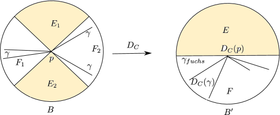
Figure 8. The map $D_{C}$ restricted to $B^{\prime}$

We call an edge of $\gamma$ any embedded sub-loop of $\gamma$, that is to say, a segment of $\gamma$ starting and ending at $p$ but not passing through $p$ appart at its extremities. Any edge is smooth outside $p$ so its image in $C_{fuchs}$ is a geodesic starting and ending at $q$. Note that any semi-geodesic in $C_{fuchs}$ starting at $\gamma_{fuchs}$ and entering the interior of $E_{fuchs}$ tends to infinity in $C_{fuchs}$ without coming back to $\gamma_{fuchs}$. It follows that $D_{C}(\gamma)\cap B\subset\overline{C_{fuchs}\setminus E}$. In particular, $\gamma\cap B^{\prime}\subset F_{1}\cup F_{2}$ (possibly the intersection is empty if $\gamma$ does not contain $p$).

Let us prove that if an exterior angle of $\gamma$ at $p$ is equal to $\pi$ or $3\pi$, then $\gamma$ passes through $p$ once. Suppose by contradiction that $\gamma$ has $s\geq 2$ edges and that the exterior angle between two consecutive edges is $\pi$ or $3\pi$. Then up to cyclic permutation of the edges, one can write $\gamma=\gamma_{1}\star\ldots\star\gamma_{s}$, where the $\gamma_{i}$’s are the edges of $\gamma$, for $i=1,\ldots,s$, and the exterior angle between $\gamma_{1}$ and $\gamma_{2}$ is $\pi$ or $3\pi$. Set $I=\gamma_{1}\star\gamma_{2}$. Then, the image of $I$ by $D_{C}$ is a union of geodesic lines contained in $\overline{C_{fuchs}\setminus E}$, passing through $q$ and forming an angle of $\pi$ at $q$. Hence $D_{C}(I)\subset\gamma_{fuchs}$ at the neighborhood of $q$. Since the image of the $\gamma_{i}$’s by $D_{C}$ are geodesic segments, this implies that the image of $\gamma_{1}$ and $\gamma_{2}$ by $D_{C}$ are some powers of $\gamma_{fuchs}$: $D_{C}(\gamma_{1})=\gamma_{fuchs}^{n_{1}}$, $D_{C}(\gamma_{2})=\gamma_{fuchs}^{n_{2}}$ for some integers $n_{1},n_{2}$. Because $D_{C}$ induces the identity on the set of free homotopy classes of loops, the loops $\gamma_{1}$ and $\gamma_{2}$ are homotopic to the loops $l^{n_{1}}$ and $l^{n_{2}}$. As $S$ is oriented, no simple loop can be a proper power, and since both $\gamma_{1}$ and $\gamma_{2}$ are embedded loops, we get $n_{1}=n_{2}=1$. But then $\gamma$ is no longer the curve minimizing the length in the free homotopy class of $l$, a contradiction.

On the other hand, if $\gamma$ passes only once through $p$, then it is a simple loop which is mapped to a geodesic loop through $q$ and in the same homotopy class as $\gamma_{fuchs}$. This shows that $D_{C}(\gamma)=\gamma_{fuchs}$ and that $(D_{C})|_{\gamma}$ is in fact an embedding. It follows that the angles that $\gamma$ forms at $p$ are $\pi$ on one side and $3\pi$ on the other.

It remains to prove the last claim. Since the exterior angles are always in $[\pi,3\pi]$, we proved that if $\gamma$ passes through $p$ at least twice, then the exterior angles of $\gamma$ at $p$ belong to $(\pi,3\pi)$. Hence, because $\gamma\cap B^{\prime}\subset F_{1}\cup F_{2}$, any exterior angle of $\gamma$ must cover one of the $E_{i}$. Because these angles at $p$ are disjoint, their number cannot exceed $2$. ∎

Let $\widehat{l}$ be a lift of $l$ in the boundary of $\widehat{C}$ and $\alpha\in\pi_{1}(C)$ be the generator of the group stabilizing $\widehat{l}$ in $\pi_{1}(C)$ that acts as a positive translation on $\widehat{l}$ for the orientation of $\widehat{l}$ given by the $\mathbb{R}\mathbb{P}^{1}$-structure of $\widehat{l}$. Since $l$ is loxodromic, we can use the upper half-plane model for $\mathbb{H}^{2}$, and choose the developing map in such a way that for some real number $\lambda>1$

$$D\circ\alpha=\lambda D$$

on $\widehat{l}$. That is to say, $\rho(\alpha)(z)=\lambda z$.

The map $D$ induces a decomposition $\widehat{l}=D^{-1}(0)\cup D^{-1}(\mathbb{R}^{>0})\cup D^{-1}(\infty)\cup D^{-1}(\mathbb{R}^{<0})$ which is $\alpha$-invariant. Since $l$ is of index $1$, the parts $\pi(D^{-1}(0))$ and $\pi(D^{-1}(\infty))$ consist of single points. We denote by $l=\{0\}\cup l^{+}\cup\{\infty\}\cup l^{-}$ the decomposition induced on $l$ (see Figure 9, left side). Observe that the map $D$ induces a projective diffeomorphism between $l^{+}$ and $\mathbb{R}^{>0}$ which is well defined up to multiplication by a power of $\lambda$. The same for $l^{-}$. Hence the multiplication by $\lambda$ is well defined on $l^{+}\cup l^{-}$.

Note that because of the choice of the upper half-plane model, we have $E_{fuchs}$ is half of $\lambda\backslash\mathbb{H}^{2}$, and $\gamma_{fuchs}$ lifts to the imaginary axis of the upper half-plane.

Proposition 7.8 (Existence of a half-bubble).

If $D_{C}(p)$ belongs to $\gamma_{fuchs}$, and $\gamma$ passes through $p$ exactly once, then for each $u\in l^{+}$ there exists a half bubble in the direction of $l$ whose endpoints in $l$ are $(u,u/\lambda)$.

Figure 9. The curve $l$ oriented counterclockwise, and its lift $\widehat{l}$

Proof.

By Lemma 7.7 $\gamma$ forms at $p$ angles $\pi$ and $3\pi$. Since $l$ has index $1$ it follows that the angle $G$ on the side of the end is the one of $3\pi$. Otherwise we would be able to move the singularity out of the end, which is in contradiction with the index hypothesis and corollary 4.6. Hence, the restriction of $D$ to $G$ covers twice the exterior angle of $\gamma_{fuchs}$ in $C_{fuchs}$ (which is the sector $E$ of Figure 8).

Let $\widehat{p}$ be a lift of $p$ in $\widehat{C}$. In the upper half-plane model of $\mathbb{H}^{2}$ that we are using, the point $D(\widehat{p})$ belongs to the positive imaginary axis. Since $l$ has index $1$, the segment from $0$ to $D(\widehat{p})$ has two pre-images joining $\widehat{p}$ to two consecutive elements of $D^{-1}(0)$ that bound a segment $J$ in $\widehat{l}$ which is a fundamental domain for the action of $\alpha$ (see Figure 9).

Let $u$ be a point of $l^{+}$ and $\widehat{u}$ be its lifts in $J$. The point $D(\widehat{u})$ belongs to the positive real line by definition of $l^{+}$. Let $\widetilde{\tau}$ be a geodesic in $\mathbb{H}^{2}$ from $D(\widehat{p})$ to $D(\widehat{u})$, and let $\tau$ be its projection to $E_{fuchs}\subset\lambda\backslash\mathbb{H}^{2}$.

By construction, $\tau$ is a geodesic in $E_{fuchs}$ starting from $q=D_{C}(p)$. As the angle of $\gamma$ at $p$ on the side of the end $E_{l}$ is $3\pi$, $\tau$ lifts to two twin geodesic paths $(\tau_{1},\tau_{2})$ in $E_{l}$, with the convention that the angle $2\pi$ is the one from $\tau_{1}$ to $\tau_{2}$ in the positive direction given by the orientation of $S$.

By Lemma 6.1 (applied with $U=\overline{E_{l}}$, $\Sigma=\overline{E_{fuchs}}\subset\lambda\backslash\mathbb{H}^{2}$, and $f=D_{C}$) the pair $(\tau_{1},\tau_{2})$ is embedded in $E_{l}$, with distinct limits at infinity $u_{1},u_{2}$. The pair $(\tau_{1},\tau_{2})$ lifts to a pair of twin geodesic $(\widehat{\tau}_{1},\widehat{\tau}_{2})$ starting from $\widehat{p}$. The arc $\tau_{1}\star\tau_{2}$ cuts $E_{l}$ — which is a topological annulus — in two parts, one of which is a disc. Since the angle from $\tau_{1}$ and $\tau_{2}$ is $2\pi$ and it is contained in $E_{l}$, the disc is the part going from $\tau_{1}$ to $\tau_{2}$ in the positive sense.

The disc between $\tau_{1}$ and $\tau_{2}$ lifts to a disc in $\widehat{C}$, bounded by $\widehat{\tau}_{1}\star\widehat{\tau}_{2}$ and a segment of $\widehat{l}$. Such a disc is homeomorphically mapped to $\mathbb{H}^{2}$ minus $\widetilde{\tau}$ by construction. Therefore, $(\tau_{1},\tau_{2})$ is a half-bubble.

If we show that $(u_{1},u_{2})=(u,u/\lambda)$ we are done. By construction we have $D(\widehat{\tau}_{1})=D(\widehat{\tau}_{2})=\widetilde{\tau}$. It follows that the end point $\widehat{u}_{1}$ of $\widehat{\tau}_{1}$ in $\widehat{l}$ belongs to $D^{-1}(D(\widehat{u}))$, and the same for $\widehat{u}_{2}$. Since the angle between $\tau_{1}$ and $\tau_{2}$ is $2\pi$ in the positive sense, it follows that $\widehat{u}_{1}\in J$ and $\widehat{u}_{2}\in\alpha(J)$. In particular, $\widehat{u}_{1}=\widehat{u}$, hence $u_{1}=u$ as we needed. Also, the point $\widehat{u}_{2}$ is the successor of $\widehat{u}_{1}$ w.r.t. the ordering of $D^{-1}(D(\widehat{u}))$ induced by $\widehat{l}$. From the fact that $l$ has index $1$ we get that when restricted to $[\widehat{u},\alpha(\widehat{u})]$ (which is a fundamental domain for the action of $\alpha$ on $\widehat{l}$) the map $D$ starts from $D(\widehat{u})$, makes a whole turn around $\mathbb{RP}^{1}$ and finally covers the fundamental domain $[D(\widehat{u}),\lambda D(\widehat{u})]$. (See Figure 9.) It follows that, according to our notation for the multiplication by $\lambda$ on $\widehat{l}$, $\widehat{u}_{2}=\lambda^{-1}\alpha(\widehat{u}_{1})$. So $u_{2}=u_{1}/\lambda=u/\lambda$. This ends the proof of Proposition 7.8. ∎

Lemma 7.9.

By moving $p$ in $C$ we can reduce to the case that $\gamma$ passes through $p$ precisely once, and $D_{C}(p)\in\gamma_{fuchs}$.

Proof.

Suppose that $\gamma$ passes twice through $p$. Let $\widehat{\gamma}$ be the lift of $\gamma$ to $\widehat{C}$ corresponding to $\widehat{l}$ (so that $\alpha$ acts by translations on $\gamma$). We look at the developed image $D(\widehat{\gamma})$. It draws a “zig-zag” line in $\mathbb{H}^{2}$. More precisely, let $\widehat{p}$ be a lift of $p$ so that $\widetilde{q}=D(\widehat{p})$ belongs to the imaginary axis in our upper half-plane model. Since $\gamma$ consists of two segments, $D(\widehat{\gamma})$ starts from a lift $\widetilde{q}$ in the imaginary axis, goes to some point $\widetilde{r}$, comes back to $\lambda\widetilde{q}$ and then repeats the same path, multiplied by $\lambda,\lambda^{2},...$. (See Figure 10, left side.)

Figure 10. The “zig-zag” line $D(\widehat{\gamma})$ and the local picture near $p$

If we look at $D_{C}(\gamma)$, we see that the two segments emanating from $D_{C}(p)$ does not enter the end $E_{fuchs}$, by the usual argument that a geodesic cannot enter and exit $E_{fuchs}$. Translated to the universal covering, this says that the point $\widetilde{r}$ belongs to the interior of the left quadrant, i.e. its real part is negative. It follows that the angles that we see on the right-side of $D(\widehat{\gamma})$ are, alternatively bigger than $\pi$ (at the points $\widetilde{q},\lambda\widetilde{q},\ldots$) and smaller than $\pi$ (at the points $\widetilde{r},\lambda\widetilde{r},\ldots$).

Let $\widehat{s}$ be the point of $\widehat{\gamma}$ such that $D(\widehat{s})=\widetilde{r}$. Denote by $\Theta$ the exterior angle seen on the right of $\widehat{\gamma}$ at $\widehat{s}$, and set $\theta=\measuredangle\widetilde{q}\widetilde{r}(\lambda\widetilde{q})<\pi$. As $D$ is a double branched covering at $\widehat{s}$, either $\Theta=\theta$ or $\Theta=2\pi+\theta$, and since $\Theta$ must exceed $\pi$ we get $\Theta=2\pi+\theta$. Moreover, since $\gamma$ passes twice through $p$, locally at $p$ we see the angular sector $\Theta$, plus the sector $\Omega$ which corresponds to the exterior angle at $\widetilde{q}$. Figure 10, right side, shows a local picture in which the angles we see on the paper are half of those around $p$ (so segments forming an angle $\pi$ represent twin segments). Since $\Theta$ and $\Omega$ are disjoint by Lemma 3.12, there exist a pair of twin geodesic segments $\tau_{1}$ and $\tau_{2}$ starting from $p$ and pointing into $\Theta$, and both lying in the complement of $\Omega$ (for instance the paths obtained as preimages of the bisector of $\theta$). Such segments are in $E_{l}$ because the angular sector $\Theta$ is that on the side of $E_{l}$.

For $i=1,2$ let $\widehat{\tau}_{i}$ be the lift of $\tau_{i}$ starting at $\widehat{s}$ and let $\widetilde{\tau}=D(\widehat{\tau}_{i})$. We have that $\widetilde{\tau}$ points in the angular sector $\theta$ because $\tau_{i}$’s are in $\Theta$. Similarly, if $\widehat{\tau}_{i}^{\prime}$ is the lift of $\tau_{i}$ that starts at $\widehat{p}$, then $D(\widehat{\tau}_{1}^{\prime})=D(\widehat{\tau}_{2}^{\prime})$ points left as in Figure 10, left side because $\tau_{i}$’s are in the complement of $\Omega$. Therefore we can geodesically extend $\widetilde{\tau}$ until the imaginary axis, without intersecting $D(\widehat{\gamma})$ nor $D(\widehat{\tau}^{\prime}_{i})$.

Since $\tau_{1}$ and $\tau_{2}$ both enter $E_{l}$, they never exit $E_{l}$. By construction $\lambda\widetilde{\tau}\cap\widetilde{\tau}=\emptyset$. So, it projects to a segment $\tau$ in $\lambda\backslash\mathbb{H}^{2}$. Now, we consider the map $D_{E}:E_{l}\to\lambda\backslash\mathbb{H}^{2}$ induced by the developing map. Lemma 6.1, applied with $U$ the open end $E_{l}$, $\Sigma=\lambda\backslash\mathbb{H}^{2}$, and $f=D_{E}$ tells us that in fact $(\tau_{1},\tau_{2})$ are embedded twin paths.

We claim that after the moving along such twin paths, we reduce to the case that $\gamma$ passes only once through $p$, and $D_{C}(p)\in\gamma_{fuchs}$. For that, we have to focus on the “zig-zag” line. Since any vertex of the “zig-zag” is the image of a lift of $p$, we see at any vertex the image of $\widetilde{\tau}$ via a certain element of $\rho(\pi_{1}(C))$. Namely, at $\lambda^{n}\widetilde{r}$ we see $\lambda^{n}\widetilde{\tau}$ and at $\lambda^{n}\widetilde{q}$ we see $\lambda^{n}D(\widehat{\tau}_{1})$.

Now, we parameterize $\tau$ with times $t\in[0,1]$ and perform the cut and paste procedure continuously on $t$. With the same notation we are using, we put an index $t$ at the bottom of every object to mean its evolution at time $t$. Namely, $\gamma_{t}$ is the geodesic representative of $l$, and $\widehat{\gamma}_{t},\widetilde{r}_{t},\widetilde{q}_{t}$ are the corresponding of $\widehat{\gamma},\widetilde{r},\widetilde{q}$ and so on. By the uniqueness of the geodesic representative of $l$ we get that $\gamma_{t}$ changes continuously on $t$. It follows that, as far as the angles that $\gamma_{t}$ forms at $p_{t}$ are bigger than $\pi$, the developed image of $\widehat{\gamma}_{t}$ is the “zig-zag” line trough $\widetilde{q}_{t},\widetilde{r}_{t},\lambda\widetilde{q}_{t},\lambda\widetilde{r}_{t}...$, which are nothing but the point $\widetilde{\tau}(t)$ and its images. Since $\widetilde{r}_{t}$ moves right and $\widetilde{q}_{t}$ moves left, eventually $\widetilde{q}$ and its images detach from $D(\widehat{\gamma}_{t})$ (in fact one can easily check with some elementary hyperbolic trigonometry, that $\Theta_{t}$ increases on $t$ while $\Omega_{t}$ decreases, and there is a time $t_{0}$ where $\Omega_{t}$ becomes $\pi$). From this time on, $\gamma_{t}$ passes through $p_{t}$ only once, and for $t=1$ the developed image of $\widehat{\gamma}_{1}$ is the imaginary axis, so $D_{C}(p_{1})\in\gamma_{fuchs}$. ∎

We remark that putting Proposition 7.8 and Lemma 7.9 together, we can directly find a (non-geodesic) half-bubble in the case where the peripheral geodesic passes twice through the branch point. This is done by considering a continuation of the path $\tau$ defined in the proof of Lemma 7.9 to a point lying in $\mathbb{R}^{+}$.

Proof of Theorem 7.1.

We consider a couple of the form $(\lambda u,u)$ in $l^{+}$. Combining Lemma 7.9 and Proposition 7.8 we show that after moving the branch points in $C^{+}$ and $C^{-}$ respectively, one can find half-bubbles $(\eta_{1}^{+},\eta_{2}^{+})$ in $C^{+}$ and $(\eta_{1}^{-},\eta_{2}^{-})$ in $C^{-}$ whose extremities are $(u_{1}^{+},u_{2}^{+})=(\lambda u,u)$ and $(u_{1}^{-},u_{2}^{-})=(\lambda u,u)$. Since geodesics in the components meet orthogonally the real curve $S_{\mathbb{R}}$, the union of $(\eta_{1}^{+},\eta_{2}^{+})$ and $(\eta_{1}^{-},\eta_{2}^{-})$ is a pair of smooth twin paths, and the two regions between the half-bubbles is in fact projectively equivalent to $\mathbb{CP}^{1}$ minus a closed segment, hence a bubble.∎

8. Degeneration dichotomy

In this section, given a BPS with Fuchsian holonomy, we try to move all the branch points in a given component of $S^{\pm}$ to a unique branch point of high branching order. By doing this, the surface may degenerate to a nodal curve. In such a situation, the degeneration allows us to find a bubble just before degenerating. If the structure does not degenerate, we succeed in our task.

Proposition 8.1.

Let $S$ be a closed surface equipped with a BPS with Fuchsian holonomy. Let $C$ be a component of $S^{\pm}$, with $R$ branch points of angle $4\pi$. Then, either we can move branch points so that we find a bubble, or we can move all the branch points of $C$ to a single branch point of angle $2\pi(R+1)$.

Proof.

The proof goes by induction, joining one by one the branch points, the inductive step being summarized as “either we can join one more branch point or we find a bubble”.

To begin with, we choose a branch point $p_{0}$ and a positive constant $\varepsilon$ smaller than the injectivity radius of $C_{fuchs}$.

Lemma 8.2.

We can move branch points so that after the moving, for every branch point $p$

$$d(p,p_{0})<\varepsilon.$$

Proof.

Let $p$ be one of the branch points which is closest to $p_{0}$ among those with $d(p,p_{0})\geq\varepsilon$ (if any). Let $\sigma$ be a geodesic joining $p$ to $p_{0}$, and of length $d(p,p_{0})$. If $d(p,p_{0})=\varepsilon$ we just move a little $p$ so that $d(p,p_{0})<\varepsilon$. Otherwise, let $\delta=d(p,p_{0})-\varepsilon>0$. The initial segment of $\sigma$ of length $\delta$ does not contain any other branch point because of the criteria for choosing $p$.

By Lemma 6.2 we can move $p$ along an initial segment of $\sigma$ of length at least $\min\{\varepsilon,\delta\}$. A recursive argument proves the claim. ∎

We denote by $D_{B}$ a developing map from $B(p_{0},\varepsilon)$ to a disc of radius $\varepsilon$ in $\mathbb{H}^{2}$. Up to little movements, we can assume that distinct branch points have distinct images and distances from $p_{0}$. At the beginning of the our strategy all conical angles are $4\pi$, but when we join a branch point to $p_{0}$ its angle increases. So we consider the general situation where the angle at $p_{0}$ is $2k\pi$.

Let $p$ be the branch point (other than $p_{0}$) closest to $p_{0}$ and $\sigma$ be a path realizing the distance from $p_{0}$ to $p$. The dichotomy is now the following:

1. There are at least two shortest paths $\sigma_{0}$ and $\sigma_{1}$ from $p_{0}$ to $p$ (and in this case our claim is that up to moving branch points one founds a bubble).

2. $\sigma$ is the unique path from $p_{0}$ to $p$ minimizing the distance (and we claim that in this case one can join $p$ to $p_{0}$).

Suppose we are in the first case. Paths $\sigma_{0}$ and $\sigma_{1}$ are both embedded otherwise there would exist a short-cut from $p$ to $p_{0}$. For the same reason, if $\sigma_{0}(t)=\sigma_{1}(s)$ for some $s,t>0$, then $s=t$. If $\sigma_{0}(t)=\sigma_{1}(t)$, for some $t>0$ then $\sigma_{0}(t)=\sigma_{1}(t)$ is not a branch point because $p$ is the closest to $p_{0}$, and also in this case we easily find shortcuts, as one of the angles between $\sigma_{0}$ and $\sigma_{1}$ is smaller than $\pi$. Therefore $\sigma_{0}$ and $\sigma_{1}$ do not cross each other.

The images $D_{B}(\sigma_{0})$ and $D_{B}(\sigma_{1})$ are therefore smooth geodesics in a disc, thus they are segments. In particular, they both are the only segment between $D_{B}(p)$ and $D_{B}(p_{0})$. Therefore $\sigma_{0}$ and $\sigma_{1}$ are twin. It follows that the loop $\sigma_{0}\sigma_{1}^{-1}$ has trivial holonomy, hence it is homotopically trivial in $S$ because the holonomy is faithful. Thus it bounds a disc $Q$ in $S$. Note that by moving $p$ along $\sigma_{0}\cup\sigma_{1}$ we would disconnect $S$.

The angle that $p_{0}$ forms on the side of $Q$ is $2h\pi$ with $h<k$. If $h>1$, we move a little $p_{0}$ using twin paths $\tau_{0},\tau_{1}$ contained in the interior of $Q$ so that, if $\sigma_{0},\tau_{0},\tau_{1},\sigma_{1}$ are in cyclic order in $Q$, then the angles $\alpha_{a}=\angle(\sigma_{0},\tau_{0})$ and $\alpha_{1}=\angle(\tau_{1},\sigma_{1})$ satisfy $\alpha_{0}+\alpha_{1}=2\pi$. This separates $p_{0}$ in $2$ branch points. One of them, which we still denote $p_{0}$, is the end-point of $\sigma_{0}$ and $\sigma_{1}$, and has an angle $2\pi$ on the side of $Q$, the other has a total angle $2(h-1)\pi$ and belongs to the interior of $Q$. We repeat the same construction outside $Q$ so to obtain that $p_{0}$ has a total angle $4\pi$, with $2\pi$ in $Q$, and $2\pi$ outside $Q$.

We cut $S$ along $\sigma_{0}\cup\sigma_{1}$ and glue the boundary of the disc $Q$ along $\sigma_{0}\cup\sigma_{1}$ by gluing $\sigma_{1}(t)$ to $\sigma_{0}(t)$. The result is a sphere $P$ with a branched projective structure, a marked segment $\sigma$ with marked end-points $p_{0}$ and $p$, both being regular. Similarly, on the other piece of $S$ we get a surface $\bar{S}$ with a market segment $\sigma$ with regular end-points $p_{0}$ and $p$.

Now, via movings, we split any branch point present in $Q$ in some number of $4\pi$-points. We obtained a branched covering $\mathbb{CP}^{1}\to\mathbb{CP}^{1}$ with branch-order at most two at any point. By moving a little branch points we can assure that they have distinct images (hence they are “simple”, with the terminology of [15].) The space of simple branched coverings from $\mathbb{CP}^{1}$ to itself is connected ([15], see for instance [11, Thm 1.54, p. 34] for a proof). A detailed account on the topology under consideration can be found in the Appendix. By Corollary 4.2 we know that the number of branch points is even. Thus we can easily construct a BPS $P_{1}$ which is branched covering $\mathbb{CP}^{1}\to\mathbb{CP}^{1}$, with the same number of branch points as $P$, by consecutive bubblings.

By Corollary 2.11, applied with $A=S$, $B=\bar{S}$, $C=P$ and $D=P_{1}$, the structure on $S$ is connected by moving branch points to a cut-and-paste of $\bar{S}$ and $P_{1}$ which clearly contains a bubble.

Suppose now that we are in case $(2)$. The path $\sigma$ does not contain other branch points because $p$ is the closest to $p_{0}$. If the image $D_{B}(\sigma)$ contains the image of some other branch point $q$, then we move $q$ a little away by using twin paths outside the ball $B(p_{0},d(p_{0},p))$. This implies that after the moving of $q$, the unique shortest path from $p$ to $p_{0}$ is still $\sigma$. The path $D_{B}(\sigma)$ is the straight segment in $\mathbb{H}^{2}$ from $D_{B}(p_{0})$ and $D_{B}(p)$. The segment $D_{B}(\sigma)$ has two lifts $\sigma$ and $\tau$ emanating from $p$. Since $p$ is the branch point closest to $p_{0}$, and since we are not in case $(1)$, the end-point of $\tau$ other than $p$ is regular (and it is not $p_{0}$). By applying Lemma 6.1 to $U=B(p_{0},\varepsilon)$, $\Sigma=\mathbb{H}^{2}$, and $f=D_{B}$ we deduce that$\sigma\cup\tau$ is embedded. We move $p$ by cut-and-pasting along $\sigma\cup\tau$. The result is that $p_{0}$ and $p$ join together to give a branch point of angle $2(k+1)\pi$ (keep in mind Figure 2). Now the induction on the number of branch points other that $p_{0}$ concludes the proof.

∎

We remark that we just proved that when we collapse some branch points to a single point, then the limit structure is a nodal curve (possibly with no nodal point if the limit is non-degenerate) consisting in a bps on $S$ with some branched coverings of $\mathbb{CP}^{1}$ attached to the nodal points.

9. Moving branch points to the positive part

In this section we prove the following result.

Theorem 9.1.

Let $S$ be a closed surface equipped with a BPS with Fuchsian holonomy. Then one can move branch points so that either a bubble appears or all branch points belong to $S^{+}$.

Proof.

The idea is to move one by one branch points from the negative to the positive part. During the process bubbles could possibly appear.

Proposition 9.2.

Let $\sigma$ be a BPS with Fuchsian holonomy on a closed surface $S$. If $p$ is a branch point contained in a negative component whose complement is not a union of discs, then $p$ can be moved to $S^{+}$.

Proof.

Let $C^{-}$ be a the component of $S^{-}$ containing $p$. We claim that there are two embedded twin paths $\gamma_{1},\gamma_{2}$ in $S$ starting at $p$, disjoint appart from $p$, and which end in the positive part. Hence, by moving $p$ along the $\gamma_{i}$’s, we get the desired result.

Let $C_{fill}$ be the union of $C^{-}$ and the components of $S\setminus C^{-}$ which are homeomorphic to discs; this is a proper subsurface of $S$. As $C_{fill}$ is not the whole $S$, its fundamental group is a free group. Elementary considerations show that the map $\pi_{1}(C_{fill})\rightarrow\pi_{1}(S)$ induced by the inclusion $C_{fill}\rightarrow S$ is injective. So the image of the inclusion map $\pi_{1}(C_{fill})\rightarrow\pi_{1}(S)$ is a free subgroup of $\pi_{1}(S)$. Consequently, the surface $C^{-}_{fuchs}=\rho(\pi_{1}(C_{fill}))\backslash\mathbb{H}^{2}$ is not compact and of infinite area.

The developing map induces a projective (hence a local isometry) map $D:C^{-}\rightarrow C^{-}_{fuchs}$. Let $\gamma:[0,\infty)\rightarrow C^{-}_{fuchs}$ be an injective semi-infinite geodesic path starting at $D(p)$ that goes to infinity in $C^{-}_{fuchs}$. We can suppose that $\gamma$ does not contain any point of the form $D(q)$ where $q$ is a branch point of $C^{-}$, other than $D(p)$ – to ensure that we can change $p$ to a branch point $q$ so that $D(q)$ is the last point of this form that $\gamma$ encounters.

The geodesic $\gamma$ can be lifted to twin paths $\gamma_{i}:[0,\infty)\rightarrow C^{-}$ starting at $p$, with $i=1,2$, such that $D(\gamma_{i})=\gamma$. By Lemma 6.1 the images of $\gamma_{1}$ and $\gamma_{2}$ are disjoint appart from $p$ and they have distinct end-points on $S_{\mathbb{R}}$. So we can move $p$ by cut and pasting anlog such twins paths and bring $p$ to $S^{+}$. ∎

It remains to deal with the case that $S\setminus C^{-}$ is a union of discs. By Proposition 8.1 either we find a bubble or we can join together all the branch points belonging to the same components.

Proposition 9.3.

Let $C$ be a negative (resp. positive) component with a single branch point $p$ of angle $2\pi(R+1)$. Suppose that $\partial C$ has a component $l$ which is homotopically trivial in $S$. Then there exist two embedded twin paths starting at $p$ with extremities in the positive (resp. negative) component having $l$ in its boundary.

Proof.

We begin by some easy preliminaries on convex subsets of $\mathbb{H}^{2}$. Suppose that $\mathcal{C}$ is a compact convex set in the upper-half plane, with piecewise geodesic boundary. A vertex of $\mathcal{C}$ is a point $v$ of $\partial\mathcal{C}$ such that the boundary makes an exterior angle bigger than $\pi$ at $v$. We denote such an exterior angular domain by $[\theta,\theta^{\prime}]\subset\mathbb{R}/2\pi\mathbb{Z}$, and we introduce the angular domain $B=[\theta+\frac{\pi}{2},\theta^{\prime}-\frac{\pi}{2}]$ at $v$.

Lemma 9.4.

Let $\gamma_{1}$ and $\gamma_{2}$ be distinct semi-infinite geodesic rays starting at some vertices $v_{1}$ and $v_{2}$ of $\mathcal{C}$ in the angular domains $B_{1}$ and $B_{2}$. Then $\gamma_{1}$ and $\gamma_{2}$ are disjoint, and their limit at infinity are different. Moreover, each $\gamma_{i}$ does not intersect $\mathcal{C}$ appart at $v_{i}$.

Proof.

By convexity of $\mathcal{C}$, it is clear that $\gamma_{1}$ and $\gamma_{2}$ do not intersect $\mathcal{C}$ appart at $v_{1}$ and $v_{2}$. If $v_{1}=v_{2}$, the first statement of the lemma is clear. Suppose now that $v_{1}\neq v_{2}$. If $\gamma_{1}$ and $\gamma_{2}$ intersect in a point $p$ (even if this point is at infinity), then the triangle $v_{1}v_{2}p$ has two angles not smaller than $\pi/2$, which violates the fact that the sum of the angles of a triangle in the hyperbolic plane is strictly less than $\pi$ if the points are not on a same line. ∎

Lemma 9.5.

The sum of the angles of $B_{v}$ over all vertex $v$ of $\mathcal{C}$ equals $2\pi+\mathrm{Area}(\mathcal{C})$.

Proof.

By Gauss-Bonnet formula, the sum of the interior angles of $\mathcal{C}$ is equal to $(k-2)\pi-\mathrm{Area}(\mathcal{C})$, where $k$ is the number of vertices of $\mathcal{C}$. Because the angle of $B_{v}$ of a vertex $v$ equals $\pi$ minus the interior angle at $v$, we deduce the formula. ∎

We are now able to finish the proof of Proposition 9.3. We suppose $C\subset S^{-}$. The case $C\subset S^{+}$ has the same proof with roles of $S^{+}$ and $S^{-}$ switched. Let $\gamma$ be the peripheral geodesic associated to $l$, and let $E$ be the end corresponding to $\gamma$. Recall (see Lemma 3.12) that $E$ is an open Annulus bounded by $\gamma$ which may be not embedded as it may self-intersect at $p$. The universal covering $\tilde{E}$ of $E$ is a half-plane delimited by a lift $\tilde{\gamma}$ of $\gamma$. Since $l$ has trivial holonomy, a developing map $D$ for the BPS of $S$ induces a well-defined projective map from $E$ to $\mathbb{H}^{2}$ which is a local isometry. Also, this map lifts to a map, still called $D$, from $\tilde{E}$ to $\mathbb{H}^{2}$ which extends to $\partial\tilde{E}$. The image of $\partial\tilde{E}$ is a closed polygonal $D(\tilde{\gamma})$ that agrees with the developed image of a lift of $\gamma$. The vertices of such a polygon are images of lifts of $p$. In particular, since there are at least two vertices, $\gamma$ is not embedded.

Let $A_{1},\ldots,A_{k}$ be the exterior (i.e. contained in $E$) angular domains of $\gamma$ at $p$. Each $A_{i}$ is mapped to an angular domain of $\mathbb{H}^{2}$ at some vertex of $D(\tilde{\gamma})$ delimited by two half-geodesics. Such geodesics cut $\mathbb{H}^{2}$ into two angular domains, a large one $L_{i}$ and a small one $S_{i}$. Since the angle of $A_{i}$ is at least $\pi$, the image of $A_{i}$ by $D$ is $L_{i}$.

Let $\mathcal{C}$ be the convex hull of $D(\tilde{\gamma})$. Suppose first that $\mathcal{C}$ has non-empty interior. For each vertex $v$ of $\mathcal{C}$, denote by $B_{v}$ the domain constructed just before Lemma 9.4. Each vertex $v$ of $\mathcal{C}$ is a point of the form $D(p_{i})$ for some lift $p_{i}$ of $p$. Moreover, by the preceeding observation, the image of $A_{i}$ contains the angular domain $B_{v}$. Let us consider pre-images $C_{v}\subset A_{v}$ so that $D(C_{v})=B_{v}$. Hence $C_{v}$ is an angular domain contained in the exterior angle $A_{i}$ of $\gamma$ at $p$.

By Lemma 9.5, the sum of the angles of the domains $B_{v}$ is larger than $2\pi$. Hence, because the angle $C_{v}$ is equal to the angle $B_{v}$, their sum exceeds $2\pi$. Thus a developing map at $p$ must overlaps some of the $C_{v}$ because of the pigeon hole principle. This shows that there exists two geodesic rays $\gamma_{1}$ and $\gamma_{2}$ starting at $p$, which are contained in the union of the domains $C_{v}$, and differing by a multiple of $2\pi$. Hence $\gamma_{1}$ and $\gamma_{2}$ are twin. Moreover, they cannot be contained in the same $C_{v}$ because twin geodesics make angle at least $2\pi$ and any $B_{v}$ is strictly less than $\pi$. Hence we can suppose that $\gamma_{1}$ starts in $A_{1}$ and $\gamma_{2}$ in $A_{2}$.

We claim that these half-geodesic rays stay in $E$, do not intersect, and tend to different points of $l$ at infinity. The images $D(\gamma_{1})$ and $D(\gamma_{2})$ are two half-geodesic rays in $\mathbb{H}^{2}$ that do not intersect by Lemma 9.4, even at infinity, and never intersect $\mathcal{C}$ appart from their starting point. Lemma 6.1 concludes.

Hence, the paths $\gamma_{1}$ and $\gamma_{2}$ can be analytically extended across $c$, ending in the positive disc, and the proposition is proved in the case $\mathcal{C}$ has non empty interior.

In the case where $\mathcal{C}$ is of empty interior, it is a geodesic segment with distinct endpoints $q_{1}$ and $q_{2}$. Sectors $B_{1}$ and $B_{2}$ measure exactly $\pi$. Therefore there exists sectors $B_{1}^{\prime}$ and $B_{2}^{\prime}$ each strictly larger than $\pi$ so that the conclusion of Lemma 9.4 holds, and the proof goes now as in the general case. This ends the proof of Proposition 9.3. ∎

An induction based on Propositions 9.2 and 9.3 proves Theorem 9.1.∎

10. Debubbling BPS with all branch points in the positive part

In this section, we consider a BPS $\sigma$ with Fuchsian holonomy on a closed compact surface $S$, having branch points only in the positive part, and we show that such a structure can always be debubbled provided it has some branch point.

Theorem 10.1.

Let $S$ be a closed surface equipped with a BPS with Fuchsian holonomy. Suppose that all branch points of $S$ belong to $S^{+}$. Then, if there is at least one branch point, we can move branch points so that the resulting BPS is a bubbling of another BPS with the same holonomy.

Proof.

Fix a positive component $C$, let $k$ be the number of branch points in $C$, and $n$ be the number of negative discs $D_{1},\ldots,D_{n}$ adjacent to $C$. Let $l_{i}=\partial D_{i}$, with the orientation induced by $C$.

Lemma 10.2.

The index of any $l_{i}$ is $1$, while the index of any other component of $\partial C$ is $0$.

Proof.

The closed disc $\overline{D_{i}}=D_{i}\cup l_{i}$ does not contain branch points, hence the developing map is a diffeomorphism from $D_{i}$ to $\mathbb{H}^{-}$, hence the index of the curve $l_{i}$ is $1$.

On the other hand, any negative component $C^{-}$ adjacent to $C$ has the structure of a complete hyperbolic surface with no cusps and, if it is different from a disc, its boundary has loxodromic holonomy. The claim follows from the index formula 4.1 applied to $C^{-}$. ∎

Lemma 10.3.

$k=2n$.

Proof.

By Lemma 10.2, the index formula applied to $C$ gives

$$eu(\rho_{C})=\chi(C)+k-n.$$

To compute $eu(\rho_{C})$, introduce the subsurface $C^{\prime}=C\cup\overline{D_{1}}\cup\ldots\cup\overline{D_{n}}$, oriented with the orientation of $S$. By the above considerations $C^{\prime}$ is an incompressible subsurface of $S$. Thus by remark 4.5 $eu(\rho_{C^{\prime}})=\chi(C^{\prime})$. Since the twisted bundle $C^{\prime}\times_{\rho}\mathbb{R}\mathbb{P}^{1}$ is trivial on the discs $D_{i}$’s , $eu(\rho_{C^{\prime}})=eu(\rho_{C})$. On the other hand, $\chi(C^{\prime})=\chi(C)+n$. We deduce that $eu(\rho_{C})=\chi(C)+n$, and the lemma follows. ∎

Let us suppose that $k$ is strictly positive. By Proposition 8.1, either we can find a bubble in $\sigma$ after moving branch points, or we can join all the branch points to a single branch point $p$ of angle $2\pi(k+1)$. For every $i=1,\ldots,n$, let $\gamma_{i}$ be the peripheral geodesic in $C$ corresponding to $l_{i}$. Since $l_{i}$ is homotopically trivial in $S$, the developed image of $\gamma_{i}$ is a closed piecewise geodesic of $\mathbb{H}^{2}$, that has at least two vertices since it is closed. Thus $\gamma_{i}$ passes at least twice through $p$. Denote by $m_{i}=m_{i}^{\prime}+2$ the number of times $\gamma_{i}$ passes through $p$, with $m_{i}^{\prime}\geq 0$, and by $\alpha^{i}_{1},\ldots,\alpha^{i}_{m_{i}}$ the exterior angles of $\gamma_{i}$ at $p$.

Lemma 10.4.

The developed image of $\gamma_{i}$ is the oriented boundary of a convex polygon $\mathcal{C}_{i}$ of $\mathbb{H}^{2}$ whose exterior angles are $\alpha^{i}_{1},\ldots,\alpha^{i}_{m_{i}}$.

Proof.

Let $y$ be a generic point of the developed image of $\gamma_{i}$ in $\mathbb{H}^{2}$ (viewed as the upper hemisphere of $\mathbb{CP}^{1}$). We consider the extremity at infinity $x_{\infty}(y)\in\mathbb{R}\mathbb{P}^{1}$ of the geodesic ray starting from $y$ in the direction normal to $\gamma_{i}$, on the right-side.

We follow $x_{\infty}$ as $y$ varies in the developed image of $\gamma_{i}$. When $y$ passes through a vertex (a developed image of $p$), we stop $y$ and let the normal vector describe the angular domain $\alpha_{j}^{i}-\pi$. As $y$ sweeps the whole developed image of $\gamma_{i}$, the point $x_{\infty}(t)$ describes a closed curve in $\mathbb{R}\mathbb{P}^{1}$ whose degree is the index of $l_{i}$. Hence, the degree of this map is $1$. Because all the angles $\alpha_{j}^{i}$ are at least $\pi$, the map $x_{\infty}(y)$ turns always counterclockwise, and this implies that $\pi\leq\alpha^{i}_{j}\leq 2\pi$ for every $j=1,\ldots,m_{i}$. This means that the developed image of $\gamma_{i}$ always turns counterclockwise, with angles $\alpha^{i}_{j}$ on its right. Because the turning number of the developed image of $\gamma_{i}$ is $1$, this implies that it bounds a convex domain of $\mathbb{H}^{2}$ on its left, ant the lemma is proved. ∎

The following result shows that there is always at least a peripheral geodesic which is not too complicated.

Lemma 10.5.

There are two possibilities:

1. either there exists a peripheral geodesic which passes through the point $p$ exactly twice,

2. or $n=1$ – equivalently $k=2$ – and the peripheral geodesic $\gamma_{1}$ passes through $p$ exactly three times.

Observe that case 1 occurs in a classical bubbling, and an example of case 2 is described in Subsection 3.5.

Proof.

The proof is based on the following Gauss-Bonnet formula: the sum of the exterior angles of a convex hyperbolic polygon with $m$ vertices equals its area plus $(m+2)\pi$. Because the union of all the exterior angles of the $\gamma_{i}$’s in the angular domain at $p$ are disjoint, we get

$$\sum_{1\leq i\leq n}(m_{i}+2)\pi+\mathrm{Area}(\mathcal{C}_{i})\leq 2\pi(k+1).$$

Dividing by $\pi$, by Lemma 10.3 and the relations $m_{i}=m_{i}^{\prime}+2$, we get

(3) $$\sum_{1\leq i\leq n}m_{i}^{\prime}+\frac{1}{\pi}\sum_{1\leq i\leq n}\mathrm{Area}(\mathcal{C}_{i})\leq 2.$$

If there exists $i$ such that $\mathrm{Area}(\mathcal{C}_{i})>0$, then $\sum_{1\leq i\leq n}m^{\prime}_{i}\leq 1$ and we infer that either one of the $m_{i}^{\prime}$’s vanishes, and we are in case (1), or all are positive, and we are in case (2). Suppose for a contradiction that $\mathrm{Int}(\mathcal{C}_{i})=\emptyset$ for all $i$, $\sum_{1\leq i\leq n}m^{\prime}_{i}\leq 2$ and $(1)$ or $(2)$ hold. Then we are necessarily in one of the following cases

1. $n=1$ (and $k=2$) and $m_{1}^{\prime}=2$,

2. $n=2$ (and $k=4$) and $m_{1}^{\prime}=m_{2}^{\prime}=1$.

Since all the $\mathcal{C}_{i}$ have empty interior, the developed images of the $\gamma_{i}$’s are segments. Therefore they must have at least two exterior angles of $2\pi$. Since exterior angles are at least $\pi$, in both cases we see that the sum of the $\alpha_{i}^{j}$’s equals the total angle around $p$. In case (a) we have angles $\alpha^{1}_{1},\alpha^{1}_{2},\alpha^{1}_{3},\alpha^{1}_{4}$ equal to $2\pi,2\pi,\pi,\pi$, and therefore they sum up to $6\pi=2(k+1)\pi$; in case (b) we must have angles $\alpha^{i}_{1},\alpha^{i}_{2},\alpha^{i}_{3}$ equal to $2\pi,2\pi,\pi$ for $i=1,2$, and they sum up to $10\pi=2(k+1)\pi$. Therefore the ends corresponding to $l_{i}$ fill the whole of $C$. In particular in case (a) the four petals of $\gamma_{1}$ are identified in pairs, whereas in case (b) the petals of $\gamma_{1}$ and $\gamma_{2}$, which are each homeomorphic to a bouquet of $3$ circles, are identified in pairs of circles, so that in fact the union $\gamma_{1}\cup\gamma_{2}$ is a bouquet of three circles. If we denote by $E_{i}$ the annular end corresponding to $\gamma_{i}$, we deduce that $S=E_{1}\cup D_{1}\cup\gamma_{1}$ in case (a); and $S=E_{1}\cup E_{2}\cup D_{1}\cup D_{2}\cup\gamma_{1}\cup\gamma_{2}$ in case (b). In both cases the characteristic of $S$ is zero, hence $S$ is a torus, which does not carry Fuchsian representations. Hence we get the desired contradiction. ∎

Lemma 10.6.

Suppose that there is a peripheral geodesic $\gamma\in\{\gamma_{1},\dots,\gamma_{n}\}$ which passes only twice through the point $p$. Then, by moving $p$, one finds a bubble.

Proof.

In this case $\gamma$ is a bouquet of two circles. Moreover, since the developed image of $\gamma$ is a segment, this bouquet is formed by two pairs of twin geodesics emanating from $p$. Let $(\nu_{1}^{1},\nu_{1}^{2})$ and $(\nu_{2}^{1},\nu_{2}^{2})$ be their germs at $p$, around the two angles $\alpha_{1}$ and $\alpha_{2}$. Let us move the multiple branch point $p$ along both twin paths. If the angle around $p$ is $2(k+1)\pi$, the structure resulting from these movements has three distinct branch points $p^{\prime},p_{1},p_{2}$. The point $p^{\prime}$ has angle $2(k-1)\pi$ (since $k=2n$, we always have $(k-1)\geq 1$, and $p^{\prime}$ is a smooth point if $k=2$); the points $p_{1}$ and $p_{2}$ are both of angle $4\pi$ and correspond to the extremities of $\nu_{1}^{i}$’s and $\nu_{2}^{i}$’s respectively. The peripheral geodesic corresponding to $l$ for this new structure is formed by two geodesic segments going from $p_{1}$ to $p_{2}$. The exterior angle are $2\pi$ at each point $p_{i}$. Hence, since $l$ bounds a disc in $S^{-}$, we are in the situation of a bubbling. ∎

Lemma 10.7.

Suppose that $n=1$ and that $\gamma_{1}$ passes through $p$ three times. Then one can move branch points so that a bubble appears.

Proof.

Let $D_{1}$ be the negative disc bounded by $l_{1}$. By Proposition 9.3, we can find two embedded twin geodesics $\nu_{1}$ and $\nu_{2}$ starting from $p$ and going in $D_{1}$, in such a way that they stay in the end corresponding to $l_{1}$ untill they cross $l_{1}$. We move $p$ along these two geodesics.

The resulting branched projective structure has the following properties. The disc $D_{1}$ gives raise to a negative annulus $A^{-}$, with a single branch point of angle $4\pi$. The component $C$ gives raise to one or two components whose union $C^{+}$ contains a single branch point of angle $4\pi$ and so that $\partial A\subset\partial C^{+}$. Lemma 10.2 and Theorem 4.1 assures that Theorem 7.1 apply in the present case and the proof is complete. ∎

The proof of Theorem 10.1 is now complete.∎

11. Proof of Theorem 1.1

First we prove that we can assume that the representation $\rho$ is Fuchsian.

Proposition 11.1.

Suppose that $\rho$ and $\rho^{\prime}$ are two representations whose actions on the Riemann sphere are topologically conjugated. Then for every $k\geq 0$, the spaces $\mathcal{M}_{k,\rho}$ and $\mathcal{M}_{k,\rho^{\prime}}$ are homeomorphic.

Proof.

Let $\Phi$ be a homeomorphism of $\mathbb{CP}^{1}$ such that $\rho^{\prime}(\cdot)\circ\Phi=\Phi\circ\rho(\cdot)$. Then, if $(S,\sigma)\in\mathcal{M}_{k,\rho}$, there is a unique developing map $D:\widetilde{S}\rightarrow\mathbb{CP}^{1}$ which is $\rho$-equivariant. Observe that the map $\Phi\circ D$ is $\rho^{\prime}$-equivariant, and define a BPS $(S,\sigma^{\prime})$ with holonomy $\rho^{\prime}$ and $k$ branch points. The correspondance $(S,\sigma)\in\mathcal{M}_{k,\rho}\mapsto(S,\sigma^{\prime})\in\mathcal{M}_{k,\rho^{\prime}}$ is the desired homeomorphism. ∎

It remains to prove that if $\rho$ is a Fuchsian representation, and $k>0$ is an integer, then $\mathcal{M}_{k,\rho}$ is connected. Let $S$ be a connected closed oriented surface, and let $\sigma$ be a branched projective structure on $S$. Suppose that $\sigma$ has holonomy $\rho$ and that it has at least one branch point.

By Corollary 4.2 we know that the number $k$ of branch points is even. Let $\Sigma$ be the uniformizing structure on $S$ with holonomy $\rho$. Let $\sigma_{0}^{k}$ be the BPS obtained by applying $k/2$ bubblings to $\Sigma$. By Corollary 2.10 this does not depend on where we perform bubblings.

We are going to prove by induction on $k$ that $\sigma$ is connected to $\sigma_{0}^{k}$ by moving branch points, and this clearly implies Theorem 1.1. The base for induction is $k=2$ as we suppose $k>0$ (for $k=0$ the claim of the theorem is false).

First, by moving a little branch points we reduce to the case that no branch point belongs to the real line $S_{\mathbb{R}}$.

By Theorem 9.1 we can move branch points so that either we find a bubble, or all branch points belong to the positive part $S^{+}$. Now, By Theorem 10.1 we find a bubble. In any case, there is a finite sequence of movements of branch points that connects $\sigma$ to a BPS $\sigma_{1}^{\prime}$ which is a bubbling on a BPS $\sigma_{1}$.

If $k>2$, by induction $\sigma_{1}$ is connected to $\sigma_{0}^{k-1}$ by moving branch points. From Corollary 2.11 applied to $A=\sigma_{1}^{\prime}$, $B=\mathbb{CP}^{1}$, $C=\sigma_{1}$, and $D=\sigma_{0}^{k-1}$, we know that $\sigma_{1}^{\prime}$ is connected to a bubbling of $\sigma_{0}^{k-1}$ and by Corollary 2.10 such a bubbling is connected to $\sigma_{0}^{k}$. In conclusion, $\sigma$ is connected to $\sigma_{0}^{k}$.

If $k=2$, then $\sigma_{1}$ has no branch points. By a celebrated theorem of W. Goldman in [7], $\sigma_{1}$ is obtained by grafting $\Sigma$ along a disjoint union of simple closed curves $\gamma_{1},\ldots,\gamma_{n}$. By moving branch points to the position of the bottom left part of Figure 6, where we put $\gamma=\gamma_{n}$, we get a BPS $\sigma_{1}^{(2)}$. By Theorem 5.1 it is precisely $\Sigma$ grafted along $\gamma_{1},\ldots,\gamma_{n-1}$ and bubbled once. We can repeat this process $n$ times to get, after appropriately moving the branch points, a BPS $\sigma_{1}^{(n)}$ that is $\Sigma$ grafted along $\emptyset$ and bubbled once, i.e. $\sigma_{0}^{2}$. ∎

12. Appendix: deformation spaces of branched projective structures

Let $S$ be a compact orientable surface of genus $g\geq 2$, equipped with a marking (i.e. an identification with the group of covering transformations of $\pi:\tilde{S}\to S$ with a fixed group $\Gamma_{g}$). Let $k$ be non-negative integer, and $\rho:\Gamma_{g}\rightarrow\mathrm{PSL}(2,\mathbb{C})$ be a non-elementary representation. In this section, we endow the set $\mathcal{M}_{k,\rho}$ of equivalence classes of BPS on $S$ with total branching order $k$ and holonomy conjugated to $\rho$, with the structure of a non-singular complex manifold of dimension $k$. In fact, we explicitly construct a complex atlas modeled on Hurwitz spaces (which inherit the complex structure from a particular space of polynomials).

We will state our main result in terms of deformations of branched projective structures, in the spririt of Kodaira-Spencer’s theory of deformations of complex manifolds, see e.g. [17].

Definition 12.1.

Let $S$ be a marked compact surface of genus $g\geq 2$. A holomorphic family of BPS on $S$ is a quadruple $(X,B,\pi,\mathcal{W})$ where

1. $X$ and $B$ are complex manifolds, $\pi:X\rightarrow B$ is a holomorphic submersion with compact fibers $S_{b}=\pi^{-1}(b)$ diffeomorphic to $S$ for all $b\in B$.

2. $\mathcal{W}=\{(U_{i},w_{i})\}$ is a maximal set of holomorphic functions $w_{i}:U_{i}\rightarrow\mathbb{CP}^{1}$ such that $\{U_{i}\}$ is an open cover of $X$, the restriction of $w_{i}$ to each fibre $S_{b}$ is non-constant and on each connected component $V$ of $U_{i}\cap U_{j}$ the functions $w_{i}$ and $w_{j}$ are related by

   $$w_{i}=\phi_{ij}(b)(w_{j})$$

   where $\phi_{ij}:\pi(V)\rightarrow\mathrm{PSL}(2,\mathbb{C})$ is a holomorphic map.

3. there is a holomorphic covering $\widetilde{X}\rightarrow X$ whose covering group is $\Gamma_{g}$ and such that over each fiber $S_{b}$, it is the universal covering of $S_{b}$.

The restriction of $\mathcal{W}$ to any fibre $S_{b}$ defines a BPS $\sigma_{b}=\mathcal{W}|_{S_{b}}$ on $S$ whose holonomy representation (up to conjugation) will be denoted by $\rho_{\mathcal{W}}(b):\Gamma_{g}\rightarrow\mathrm{PSL}(2,\mathbb{C})$.

When $(X,B,\pi,\mathcal{W})$ is a holomorphic family of BPS, we also say that $X$ is a holomorphic family of BPS over $B$, with atlas $\mathcal{W}$.

Theorem 12.2.

Given a non-elementary representation $\rho:\Gamma_{g}\rightarrow\mathrm{PSL}(2,\mathbb{C})$, there exists a smooth complex manifold structure on $\mathcal{M}_{k,\rho}$ such that, for any holomorphic family $(X,B,\pi,\mathcal{W})$ of BPS on $S$ with $k$ branch points counted with multiplicity and holonomy $\rho_{\mathcal{W}}=\rho$, the map

$$b\in B\mapsto\sigma_{b}=\mathcal{W}|_{S_{b}}\in\mathcal{M}_{k,\rho}$$

is holomorphic.

It would be interesting to endow the set $\mathcal{M}_{k}=\cup_{\rho}\mathcal{M}_{k,\rho}$ of BPS with $k$ branch points counted with multiplicity with a structure of a complex analytic space, by gluing the complex structures on $\mathcal{M}_{k,\rho}$ together. This can be done over the set of non elementary representations, but we don’t know how to manage this over the elementary representations. Some preliminaries are in order.

Let $T_{g}$ be the Teichmüller space consisting of equivalence classes of marked Riemann surfaces of genus $g$, up to biholomorphism lifting to the universal cover as a $\Gamma_{g}$-equivariant diffeomorphism. Bers equipped the set $T_{g}$ with the structure of a complex manifold of dimension $3g-3$, and constructed the tautological bundle $\Pi:\mathcal{T}_{g}\rightarrow T_{g}$ over it: a holomorphic family of marked Riemann surfaces where the fiber over a point $t\in T_{g}$ is biholomorphic to $t$. He showed that this family of Riemann surfaces is universal in the sense of Kodaira-Spencer’s deformation theory, see [3], [9, Théorème 1.2] and [1, p. 446]. Namely, if $\pi:X\rightarrow B$ is any holomorphic family of marked Riemann surfaces, then there is a holomorphic map $f:B\rightarrow T_{g}$ such that $(X,B,\pi)=f^{*}(T_{g},\mathcal{T}_{g},\Pi)$.

To prove this result Bers introduced a holomorphic family of (unbranched) $\mathbb{CP}^{1}$-structures on $\mathcal{T}_{g}$, usually called Bers simultaneous uniformization. This is the data of a holomorphic family of quasi-Fuchsian representations

$$t\in T_{g}\mapsto\rho_{t}\in\mathrm{Hom}\big{(}\Gamma_{g},\mathrm{PSL}(2,\mathbb{C})\big{)}$$

and of an open set $U\subset T_{g}\times\mathbb{CP}^{1}$ such that for every $t\in T_{g}$, the intersection $U\cap\{t\}\times\mathbb{CP}^{1}$ is of the form $\{t\}\times U_{t}$, where $U_{t}$ is a component of the domain of discontinuity of $\rho_{t}$. The set $\mathcal{T}_{g}$ is then constructed as the quotient of $U$ by the action $\gamma(t,z)=(t,\rho(t)(\gamma)(z))$ of $\Gamma_{g}$ on $U$. The projection onto the first coordinate gives a map $\Pi:\mathcal{T}_{g}\rightarrow T_{g}$ whose fiber over a point $t\in T_{g}$ is the Riemann surface structure $t$ on $S$.

Let us comment on the relationship between the two natural projections defined so far on the space of branched projective structures with total branching order $k$: the holonomy projection to the $\mathrm{PSL}(2,\mathbb{C})$-character variety and the projection to Teichmüller space. The first one provides, together with the order of branching, the stratification by the sets $\mathcal{M}_{k,\rho}$. When $k=0$, that is, on strata of unbranched projective structures, the fibres of both projections intersect transversally (in fact by Goldman’s theorem and Baba’s generalization the holonomy fibers are discrete). In this case, the holonomy and the underlying conformal structure determine the projective structure (see [23]). In the case of $0<k<2g-2$ where $g$ is the genus of the surface, it is still true that the triple, holonomy, conformal structure and branching divisor determine the branched projective structure (see [23]). Moreover, for $0<k<2g-2$, the fibers of the Teichmuller and holonomy projections are transverse: for a fixed holonomy, moving branch points changes the conformal structure. However, when $k\geq 2g-2$, there exist movements of branch points that preserve the holonomy and the conformal structure. As suggested by G. Mondello, they can be calculated directly by using the Beltrami differentials associated to moving branch points and Riemann-Roch’s formula. A consequence is that the fibres of the two projections are not transverse in this case (note that the complex dimension of the Teichmüller space of $S$ is $3g-3$ while the dimension of $\mathcal{M}_{\rho,k}$ is $k$).

Coming back to the question of existence of rational curves in $\mathcal{M}_{k,\rho}$ stated in subsection 1.1, by considering the tautological bundle associated to a rational curve, we get a holomorphic family of branched projective structures parametrized by $\mathbb{CP}^{1}$ whence the projection on Teichmüller space provides a rational curve, which must be constant, as Teichmüller space does not contain rational curves. So the rational curve must be contained on the fiber of the projection. In particular this implies $k\geq 2g-2$. The same holds true for a non trivial holomorphic family of BPS over a compact base $B$.

12.1. The deformation spaces $\mathcal{M}_{k_{1},\ldots,k_{r},\rho}$

Let $k_{1}\leq\ldots\leq k_{r}$ be positive integers such that $k_{1}+\ldots+k_{r}=k$, and $\mathcal{M}_{k_{1},\ldots,k_{r}}$ be the set of BPS on $S$ whose branch divisor is of the form $\sum_{i=1}^{r}k_{i}p_{i}$ for some set of distinct points $\{p_{1},\ldots,p_{r}\}$. The set $\mathcal{M}_{k_{1},\ldots,k_{r}}$ has a structure of an analytic space that can be defined by using the usual Schwarzian derivative parametrization. We recall this construction for convenience of the reader, see [6, 12.2, p. 679] in the case where $k_{i}=1$ for all $i$. For any BPS in $\mathcal{M}_{k_{1},\ldots,k_{r}}$, one can consider its underlying Riemann surface structure $t$ and, introducing the Bers coordinate $z\in U_{t}$ and a developing map $D$ for the given BPS, construct the meromorphic quadratic differential on $U_{t}$ defined by

(4) $$q(z):=\{D(z),z\}dz^{2},$$

where $\{D,z\}$ denotes the Schwarzian derivative. This meromorphic quadratic differential on $U_{t}$ does not depend on the choice of the developing map and is invariant by $\rho_{t}$, hence defines a meromorphic quadratic differential on $t$ that has pole set at the branch points $\{p_{1},\ldots,p_{r}\}$ of the BPS. Its Laurent series expansion around $p_{i}$ in a coordinate $z$ where $p_{i}=z_{i}$ is

(5) $$q(z)=\frac{1-(k_{i}+1)^{2}}{2(z-z_{i})^{2}}+\sum_{n\geq-1}a_{n}^{(i)}(z-z_{i})^{n}.$$

A necessary and sufficient condition on the coefficients $a_{n}$ , $n\geq-1$, ensuring that a meromorphic quadratic differential of type (5) is the quadratic meromorphic differential associated to a BPS of $\mathcal{M}_{k_{1},\ldots,k_{r}}$ as in (4), is that some polynomial equation on the coefficients $a_{n}^{(i)}$ is satisfied, called the indicial equation. This equation takes the form

(6) $$A_{k_{i}}(a_{-1}^{(i)},\ldots,a_{k_{i}-1}^{(i)})=0,$$

where $A_{k_{i}}$ is a polynomial in $k_{i}$ variables with coefficients in $\mathbb{C}$ (see [22, p. 268]).

Introduce the tautological fiber bundle $\mathcal{T}_{g}^{(r)}$ over Teichmüller space $T_{g}$, where the fibre over a point $t\in T_{g}$ is biholomorphic to the set $t^{r}\setminus\Delta(t)$ where $\Delta(t)$ is the set of $r$-tuples $(p_{1},\ldots p_{r})\in t^{r}$ such that $p_{i}=p_{j}$ for some distinct indices. Let $\mathcal{Q}_{g}^{(r)}$ be the vector bundle over $\mathcal{T}_{g}^{(r)}$ whose fiber over a point $t^{(r)}\in\mathcal{T}_{g}^{r}$ consists of those meromorphic quadratic differentials on $t^{r}$ whose poles are precisely at the $p_{i}$’s corresponding to $t^{r}$ and that satisfy equation (5). Following the preceding discussion, the set $\mathcal{M}_{k_{1},\ldots,k_{r}}$ can be identified with the subset of $\mathcal{Q}_{g}^{(r)}$ consisting of meromorphic quadratic differentials verifying the indicial equations (6). This set has the structure of a complex analytic space. Moreover, the subset of $\mathcal{M}_{k_{1},\ldots,k_{r},\rho}$ consisting of those BPS in $\mathcal{M}_{k_{1},\ldots,k_{r}}$ whose holonomy is conjugated to $\rho$ is an analytic subset. Indeed, since $\rho$ is non-elementary, $\mathcal{M}_{k_{1},\ldots,k_{r},\rho}$ is a fibre of the analytic map that associates to each $\sigma$ in $\mathcal{M}_{k_{1},\ldots,k_{r}}$ the character $\Lambda_{\sigma}:\Gamma_{g}\rightarrow\mathbb{C}$ defined by $\Lambda_{\sigma}([\gamma])=\mathrm{Tr}^{2}(\rho_{\sigma}([\gamma]))$.

The structure of complex space structure on $\mathcal{M}_{k_{1},\ldots,k_{r},\rho}$ constructed in 12.1 cannot be extended in an obvious manner to provide a complex analytic structure on $\mathcal{M}_{k,\rho}$. The reason is that the map that assigns to a BPS its number of branch points is only semi-continuous, and in fact discontinuous around points where some of the $k_{i}\geq 2$. This is reflected in the Schwarzian coordinates. For instance, given a continuous family $\sigma_{b}$ of elements in $\mathcal{M}_{k,\rho}$ where at $\sigma_{0}$ there is a branch point $p_{0}$ of multiplicity $k_{0}\geq 2$ and for all $b\neq b_{0}$ all the branch points of $\sigma_{b}$ are simple, there is a discontinuity in the family of meromorphic quadratic differentials $q_{b}$ at the point $b_{0}$: its number of poles is not constant (note that the poles of the Schwarzian are always of order two, and the information about the branching-index of a BPS is encoded in the principal coefficient of the Schwarzian, see (5)). To overcome this difficulty, we will adopt a different approach and use Hurwitz spaces to endow $\mathcal{M}_{k,\rho}$ with the structure of a complex manifold.

12.2. The smooth topology on $\mathcal{M}_{k}$

Given a point $\tau\in\mathcal{M}_{k}$ we consider its underlying complex structure on $S$ and name it $t(\tau)\in T_{g}$. Since $U_{t(\tau)}$ is the complex analytic universal covering associated to $t$, we can consider a developing map $D_{\tau}$ for $\tau$. It is tautologically a holomorphic map from $U_{\tau}$ to $\mathbb{CP}^{1}$. The smooth topology on $\mathcal{M}_{k}$ is the topology induced by the injective map $\tau\mapsto(\Gamma_{t(\tau)},D_{\tau})$ using the topology of the Bers slice one one component and the uniform convergence on compact sets for developing maps. As we let $\mathrm{PSL}(2,\mathbb{C})$ act on the space of the developing maps, it is not completely obvious that this topology on $\mathcal{M}_{k}$ (or even its restriction to $\mathcal{M}_{k,\rho}$) is Hausdorff, so we are led to introduce the topological structure differently.

12.3. Cut and paste topology on $\mathcal{M}_{k,\rho}$

We begin by introducing a topology on $\mathcal{M}_{k,\rho}$ as follows. The Riemann surface associated to a BPS in $\mathcal{M}_{k,\rho}$ is equipped with its Poincaré metric coming from uniformization. Given $\varepsilon>0$ and $\sigma\in\mathcal{M}_{k,\rho}$ define $\mathcal{V}(\varepsilon,\sigma)\subset\mathcal{M}_{k,\rho}$ as the set of elements $\sigma^{\prime}\in\mathcal{M}_{k,\rho}$ such that there exists a diffeomorphism $\Phi:S\rightarrow S$ satisfying:

1. $\Phi$ is $(1+\varepsilon)$-bi-Lipschitz with respect to the Poincaré metrics on $S$ given by $\sigma$ and $\sigma^{\prime}$ respectively,

2. $\Phi$ is projective outside the $\varepsilon$-neighborhoods of the branched set of $\sigma$,

3. $\Phi$ is isotopic to the identity.

The topology on $\mathcal{M}_{k,\rho}$ is defined as the one generated by the neighbourhoods $\mathcal{V}(\varepsilon,\sigma)$.

Lemma 12.3.

The cut and paste topology on $\mathcal{M}_{k,\rho}$ is separated.

Proof.

Suppose that $\sigma_{i}$, for $i=1,2$ are two elements of $\mathcal{M}_{k,\rho}$ that cannot be separated. This means that for every $\varepsilon>0$, there exists an element $\sigma_{\varepsilon}$ in $\mathcal{V}(\varepsilon,\sigma_{1})\cap\mathcal{V}(\varepsilon,\sigma_{2})$. By definition, for every $\varepsilon>0$, and every $i=1,2$, we have a diffeomorphism $\Phi_{\varepsilon,i}:S\rightarrow S$ such that properties 1), 2) and 3) above are satisfied w.r.t. $\sigma_{\varepsilon}$ and $\sigma_{i}$. The diffeomorphism $\Psi_{\varepsilon}=\Phi_{\varepsilon,2}^{-1}\circ\Phi_{\varepsilon,1}$ is $(1+\varepsilon)^{2}$-bi-Lipschitz, w.r.t. the metrics given by $\sigma_{1}$ and $\sigma_{2}$, is projective appart from the $\varepsilon(1+\varepsilon)^{2}$-neighborhood of the branched set of $\sigma_{1}$, and isotopic to the identity. By the theorem of Arzela-Ascoli, one can find a sequence $\varepsilon_{n}$ tending to $0$ when $n$ tends to infinity such that $\Psi_{\varepsilon}$ converges to an isometry $\Psi$ w.r.t the metrics given by $\sigma_{1}$ and $\sigma_{2}$, which is projective appart from the branched set of $\sigma_{1}$. Then $\Psi$ is projective everywhere, and it is isotopic to the identity. Hence $\sigma_{1}=\sigma_{2}$ in $\mathcal{M}_{k,\rho}$. ∎

Lemma 12.4.

Given any holomorphic family $(X,B,\pi,\mathcal{W})$ of BPS on $S$ with $k$ branch points and holonomy conjugated to $\rho$, the induced map from $B$ to $\mathcal{M}_{k,\rho}$ (endowed with the cut-and-paste topology) is continuous.

Proof.

We have to prove that given $b_{0}\in B$ and $\varepsilon>0$, there is a neighborhood of $b_{0}$ in $B$ such that for every $b$ in this neighborhood, the BPS $\sigma_{b}=\mathcal{W}|_{S_{b}}$ on $S$ belongs to $\mathcal{V}(\varepsilon,\sigma_{b_{0}})$.

Since the holonomy of $\sigma_{b}$ is always conjugated to the non-elementary representation $\rho$, there is a unique developing map $D_{b}:\widetilde{S_{b}}\rightarrow\mathbb{C}\mathbb{P}^{1}$ which is $\rho$-equivariant. The family of functions $\{D_{b}\}$ defines a holomorphic function $D:\widetilde{X}\rightarrow\mathbb{CP}^{1}$. By $\rho$-equivariance, the foliation defined by $D=\mathrm{cst}$ is invariant by the $\Gamma_{g}$-action on $\widetilde{X}$, and defines a regular holomorphic foliation $\mathcal{F}$ on $X$ which is transversally projective. By construction, the BPS on the curves $S_{b}$ is the restriction of the transversal projective structure of this foliation, (see subsection 2.2). The foliation $\mathcal{F}$ is tangent to the curves $S_{b}$ precisely at the set $B_{b}$ of branch points of $\sigma_{b}$. Hence, if we denote by $B_{b}^{\varepsilon}$ the set of points of $S_{b}$ within distance $\varepsilon$ from $B_{b}$, and if $b$ is sufficiently close to $b_{0}$, there is a family of diffeomorphisms $\Phi_{b}:S_{b_{0}}\setminus B_{b_{0}}^{\varepsilon}\rightarrow S_{b}$ depending differentiably on the parameter $b$, that preserves each leaf of $\mathcal{F}$, and such that $\Phi_{b_{0}}$ is equal to the identity. By elementary topological arguments, this family can be extended differentiably to a family of diffeomorphisms $\Phi_{b}$ between $S_{b_{0}}$ and $S_{b}$ such that $\Phi_{b_{0}}=id$. Because the Poincaré metric on the fibers $S_{b}$ varies continuously with the parameter $b$, for $b$ close enough to $b_{0}$, this family of diffeomorphisms verifies the conditions 1), 2) and 3) of the definition of $\mathcal{V}(\varepsilon,\sigma_{b_{0}})$. ∎

Corollary 12.5.

The cut-and-paste and the smooth topologies coincide on each stratum $\mathcal{M}_{k_{1},\ldots,k_{r},\rho}$.

Proof.

Let $\Pi:\mathcal{T}_{g}\to T_{g}$, $\mathcal{T}_{g}^{(r)}\to T_{g}$ and $\mathcal{Q}_{g}^{(r)}\to\mathcal{T}_{g}^{(r)}\to T_{g}$ be as before (namely, they are respectively the tautological bundle over the Teichmüller space of $S$, its $r$-th symmetric product, and a vector bundle of meromorphic quadratic differentials) so that $\mathcal{M}_{k_{1},\ldots,k_{r},\rho}$ is identified with the sub-set of $\mathcal{Q}_{g}^{(r)}$ of Schwarzian-integrable differentials with holonomy conjugated to $\rho$. Now we build a holomorphic family of BPS as follows. The base $B$ is just $\mathcal{M}_{k_{1},\ldots,k_{r},\rho}$ endowed with its smooth topology induced by $\mathcal{Q}_{q}^{(r)}$. Then, we let $X$ be the pull-back of the tautological bundle $\pi_{t}:\mathcal{T}_{g}\to T_{g}$ via the map $\mathcal{Q}_{g}^{(r)}\to T_{g}$. The set of maps $\mathcal{W}$ is given by the integral of the Schwarzian differentials. By Lemma 12.4, the identity between $\mathcal{M}_{k_{1},\ldots,k_{r},\rho}$ with the smooth topology and itself with the cut-and-paste topology is continuous. Since $\mathcal{M}_{k_{1},\ldots,k_{r},\rho}$ with the smooth topology is locally compact with countable basis, the identity is a homeomorphism between the two topologies. ∎

At this point it is worth mentioning that there is yet another viewpoint for studying branched projective structures: that of flat holomorphic connections. Namely, let $d\geq 0$ and $g\geq 2$ be integers. Consider the set of all quadruples $(C,E,\nabla,s)$ where $C$ is a compact marked Riemann surface of genus $g$ $E$ is a $\mathbb{CP}^{1}$-bundles over $C$, $\nabla$ is a flat holomorphic connexion on $E$ (equivalently a horizontal foliation $\mathcal{F}$ which is transverse to the fibers) with irreducible monodromy, and $s$ is a section which has $d$ points of tangencies with $\mathcal{F}$. This provides a BPS on the surface $C$ (as in subsection 2.2), and the space of connections provides analytic coordinates (on each stratum with a fixed number of tangencies). For details about this viewpoint we refer the reader to [10, 22, 23, 24].

12.4. Hurwitz spaces

Our goal now is to prove that $\mathcal{M}_{k,\rho}$ is locally modeled on a product of Hurwitz spaces, i.e. moduli spaces of coverings of the disc.

Definition 12.6 (Hurwitz spaces).

Let $U$ be a smooth closed disc, $\psi:U\rightarrow\mathbb{D}$ be a branched covering of degree $d$ with no critical values on the boundary, and let $f:\mathbb{S}^{1}\to\partial U$ be a diffeomorphism so that $\psi\circ f(z)=z^{d}$ on $\mathbb{S}^{1}$. We consider the set of smooth branched coverings $\psi^{\prime}:U^{\prime}\rightarrow\mathbb{D}$ of degree $d$ from a smooth closed disc $U^{\prime}$ to $\mathbb{D}$, with no critical value on the boundary, together with an identification $f^{\prime}:\partial U\to\partial U^{\prime}$ such that $\psi=\psi^{\prime}\circ f^{\prime}$ on $\partial U$ (equivalently, so that $\psi^{\prime}\circ f^{\prime}\circ f(z)=z^{d}$ on $\mathbb{S}^{1}$). Two such coverings $\psi_{i}:U_{i}\rightarrow\mathbb{D}$, $i=1,2$, are identified if the diffeomorphism $\varphi=f_{2}\circ f_{1}^{-1}$ from $\partial U_{1}$ to $\partial U_{2}$ extends to a diffeomorphism $\phi:U_{1}\rightarrow U_{2}$ such that $\psi_{1}=\psi_{2}\circ\phi$.

The set of equivalence classes under this equivalence relation is denoted by $\mathcal{H}(\psi)$, and will be called a Hurwitz space of degree $d$ coverings.

Observe that the pull-back via $\psi$ of the projective structure of $\mathbb{D}$ given by its inclusion in $\mathbb{CP}^{1}$ induces a BPS on $U$. Moreover, if $\psi_{i}$, $i=1,2$ are two elements of $\mathcal{H}(\psi)$, then the diffeomorphism $\varphi=f_{2}\circ f_{1}^{-1}:\partial U_{1}\rightarrow\partial U_{2}$ extends to a projective diffeomorphism from a neighborhood of $\partial U_{1}$ to a neighborhood of $\partial U_{2}$. The identifications of the boundaries of the discs with $\mathbb{S}^{1}$ define a marked point $1$. Namely, we set $1:=f(1)$ in $\partial U$ and $1:=f^{\prime}(1)$ in any $\partial U^{\prime}$.

We now prove that Hurwitz spaces are nicely parametrized by open sets of complex vector spaces, and this will define a natural topology on $\mathcal{H}(\psi)$.

Lemma 12.7.

Any Hurwitz space $\mathcal{H}(\psi)$ of degree $d$ coverings is a smooth complex manifold of dimension $d-1$. More precisely, $\mathcal{H}(\psi)$ is in bijection with the set of complex polynomials of the form

$$P(z)=z^{d}+a_{d-1}z^{d-1}+\ldots+a_{0}$$

with $a_{d-1}+\ldots+a_{0}=0$ and with all critical values in the interior of the unit disc.

Proof.

For every class $\psi^{\prime}$ in $\mathcal{H}(\psi)$, the disc $U^{\prime}$ is equipped with a unique Riemann surface structure such that $\psi^{\prime}:U^{\prime}\rightarrow\mathbb{D}$ is holomorphic. Let $\mathbb{D}^{c}$ be the exterior of the unit disc in $\mathbb{CP}^{1}$. We glue $U^{\prime}$ and $\mathbb{D}^{c}$ by using the identification of their boundaries given by $f^{\prime}\circ f$. We obtain a Riemann surface of genus $0$ that we denote by $\mathbb{P}_{[\psi^{\prime}]}$. The covering $\psi^{\prime}:U^{\prime}\rightarrow\mathbb{D}$ can be glued together with the covering $z\in\mathbb{D}^{c}\mapsto z^{d}\in\mathbb{D}^{c}$ to give rise to a holomorphic branched covering $\overline{\psi^{\prime}}:\mathbb{P}_{[\psi^{\prime}]}\rightarrow\mathbb{CP}^{1}$. Since the set of Möbius transformations acts freely and transitively on triples $(x,y,v)$ where $x\neq y\in\mathbb{CP}^{1}$ and $0\neq v\in T_{x}(\mathbb{CP}^{1})$, there is a unique biholomorphism $\eta:\mathbb{CP}^{1}\rightarrow\mathbb{P}_{[\psi^{\prime}]}$ such that

• $\eta(\infty)=\infty\in\mathbb{D}^{c}$;

• $\eta(1)=1\in\mathbb{S}^{1}=\partial\mathbb{D}^{c}$;

• $\overline{\psi^{\prime}}\circ\eta(w)=w^{d}+O(w^{d-1})$.

We denote by $P$ the polynomial $\overline{\psi^{\prime}}\circ\eta(w)$. By construction it satisfies the assumptions of the lemma. Reciprocally, if $P$ satisfies the assumptions of the lemma, denote by $V_{P}:=P^{-1}(\overline{\mathbb{D}})=\{z:P(z)\leq 1\}$ and let $\psi^{\prime}$ be the restriction of $P$ to $V_{P}$. Because there is no critical value of modulus $\geq 1$ apart from the point at infinity, $V_{P}$ is a disc and the covering $\psi^{\prime}:\partial V_{P}\rightarrow\partial\mathbb{D}$ is cyclic. Observe that $P(1)=1$, so that there is a unique diffeomorphism $f_{P}:\partial U\to\partial V_{P}$ such that $P(f_{P}(f(z)))=z^{d}$. ∎

Remark 12.8.

From the fact that $P(f_{P}(f(z)))=z^{d}$ we get that $P(z)=(f^{-1}\circ f_{P}^{-1}(z))^{d}$ hence $f^{-1}\circ f_{P}^{-1}(z)=\sqrt[d]{P(z)}$. It follows that $f_{P}$ depends holomorphically on the variable $P$.

12.5. A holomorphic atlas on $\mathcal{M}_{k,\rho}$ modeled on Hurwitz spaces

We begin with the following local description near a branch point $p$ of a BPS $\sigma$ on a surface $S$. Let $U$ be a disk-neighbourhood of $p$, with local complex coordinate $\zeta$ so that the map $\psi(\zeta)\to\zeta^{d}$ belongs to the atlas of $\sigma$. Choose $f:\mathbb{S}^{1}\to\partial U$ as in definition 12.6. We identify $\mathcal{H}(\psi)$ with the set of polynomials given by Lemma 12.7. For any $P\in\mathcal{H}(\psi)$ let $V_{P}=P^{-1}(\mathbb{D})$ and define the set $X\subset\mathbb{C}\times\mathcal{H}(\psi)$ by

$$X=\{(z,P)\in\mathbb{C}\times\mathcal{H}(\psi):\ z\in V_{P}\}.$$

Let $\pi:X\to\mathcal{H}(\psi)$ be the natural projection, which is clearly a holomorphic submersion with fibres $\pi^{-1}(P)=V_{P}$. Moreover, the function $w:X\to\mathbb{CP}^{1}$ given by $w(z)=P(z)\in\mathbb{D}\subset\mathbb{CP}^{1}$ defines a maximal atlas $\mathcal{W}$ so that $w\in\mathcal{W}$. Thus, $X$ can be viewed as a holomorphic family of BPS over $\mathcal{H}(\psi)$. (In our Definition 12.1 the fibres are diffeomorphic to $S$, but a similar definition can be given for families of BPS on a disk.)

The boundary $\partial X$ is a fibre bundle

$$\partial V_{P}\hookrightarrow\partial X\stackrel{{\scriptstyle\pi}}{{\to}}\mathcal{H}(\psi).$$

The identification from $\partial U\times\mathcal{H}(\psi)=\partial(U\times\mathcal{H}(\psi))$ to $\partial X$ given by $(z,P)\to(f_{P}(z),P)$ is holomorphic and extends holomorphically from a collar of $\partial U\times\mathcal{H}(\psi)$ in $U\times\mathcal{H}(\psi)$ to a collar of $\partial X$ in $X$ by Remark 12.8.

It follows that by gluing $S\setminus U\times\mathcal{H}(\psi)$ with $X$ along their common boundaries using the above identification we get a complex manifold $\mathcal{X}$ and a holomorphic submersion $\mathcal{X}\to\mathcal{H}(\psi)$ so that the fibre over $P$ is the BPS obtained from $\sigma$ by replacing $U$ with $V_{P}$. Note that, after the identification of the collars of $\partial U\times\mathcal{H}(\psi)$ and of $\partial X$, the changes of charts near $\partial U$ are the identity by Remark 12.8. The developing maps given by the atlas of $\sigma$ on $S\setminus U$ and by $(z,P)\to P(z)$ on $X$, provide an atlas $\mathcal{W}$ as requested by Definition 12.1, and since $U$ is a disk, such a construction lifts to the universal covering of $S$. Therefore, $\mathcal{X}$ is a holomorphic family of BPS over $\mathcal{H}(\psi)$.

We are now ready to describe a complex atlas of $\mathcal{M}_{k,\rho}$ modeled on a product of Hurwitz spaces by repeating the above construction around every branch point of $\sigma$.

Let $\sigma$ be a BPS on a surface $S$. For every branch point $p$ of $S$, there exists a disc neighbourhood $U_{p}$ with a complex coordinate $\zeta_{p}$ and an integer $k_{p}$ such that the branched covering $\psi_{p}(\zeta)=\zeta_{p}^{k_{p}}$ belongs to the atlas of $\sigma$. By restricting $U_{p}$ if necessary and composing $\psi_{p}$ on the left by an affine transformation, we may assume that the $U_{p}$’s are disjoint and that the image of any $\psi_{p}$ is the unit disc $\mathbb{D}\subset\mathbb{CP}^{1}$.

We denote by $\Psi:=(\psi_{p})_{p}$, $\mathcal{H}(\Psi):=\prod_{p}\mathcal{H}(\psi_{p})$, and $k=\sum_{p}k_{p}$, where the index $p$ runs over all branch points of $\sigma$. Given any element $\Psi^{\prime}:=(P_{p})_{p}\in\mathcal{H}(\Psi)$, we construct a new branched projective structure belonging to $\mathcal{M}_{k,\rho}$ by cutting off $U_{p}$ and gluing back $V_{P_{p}}$ via the identifications of the boundaries for every branch point $p$. This defines a subset of $\mathcal{M}_{k,\rho}$ that will be denoted by $\mathcal{V}(\Psi)$. This procedure defines a map $c(\Psi):\mathcal{H}(\Psi)\rightarrow\mathcal{V}(\Psi)$.

Lemma 12.9.

For every $\Psi$ as above, the set $\mathcal{V}(\Psi)$ is a neighborhood of $\sigma$ in the topology of $\mathcal{M}_{k,\rho}$.

Proof.

Since every element of $\mathcal{V}(\varepsilon,\sigma)$ is obtained from $\sigma$ by changing the projective structure only in the $\varepsilon$-neighborhood of the branch-set of $\sigma$, for a sufficiently small $\varepsilon>0$, $\mathcal{V}(\varepsilon,\sigma)\subset\mathcal{V}(\Psi)$. ∎

Lemma 12.10.

The map $c(\Psi)$ is a bijection.

Proof.

To obtain this claim it is sufficient to prove that if $\Psi^{\prime}=(P_{p})_{p}\in\mathcal{H}(\Psi)$ produces a branched projective structure $\sigma^{\prime}$ equivalent to $\sigma$, then $\Psi^{\prime}=\Psi$. If $\sigma^{\prime}$ is equivalent to $\sigma$, then there is a diffeomorphism $\Phi:S\to S$ isotopic to the identity which is projective w.r.t. $\sigma^{\prime}$ and $\sigma$ respectively. Let $U^{\prime}_{p}=\Phi(V_{P_{p}})$ and consider the inclusion $i:S\setminus\{U_{p}\}\hookrightarrow S\setminus\{V_{P_{p}}\}$, which is projective by definition. The map $h=\Phi\circ i$ is a projective diffeomorphism from $S\setminus\{U_{p}\}$ to $S\setminus\{U^{\prime}_{p}\}$ that is isotopic to the identity. It lifts to the universal covers

$$\tilde{h}:\widetilde{S}\setminus\{\widetilde{U_{p}}\}\to\widetilde{S}\setminus\{\widetilde{U^{\prime}_{p}}\}$$

as a $\Gamma_{g}$-equivariant diffeomorphism. Let $D$ be a developing map for $\sigma$. Since $\tilde{h}$ is locally a projective map, and since $\widetilde{S}\setminus\{\widetilde{U_{p}}\}$ is connected, there exists a Möbius transformation $A$ such that

$$D\circ\tilde{h}=A\circ D.$$

By $\rho$-equivariance of $D$ it follows that $A$ commutes with the image of $\rho$, hence $A=Id$ as $\rho$ is irreducible.

Now we choose local coordinates $\zeta_{p}$ near a branch point $p$ such that $D(\zeta_{p})=\zeta_{p}^{k_{p}}$. We get $(\tilde{h}(\zeta_{p}))^{k_{p}}=\zeta_{p}^{k_{p}}$ which implies that $\tilde{h}$ can be analytically extended to the whole $\tilde{S}$. So $h$ extends to a biholomorphism of $S$. Since $h$ is isotopic to the identity and $S$ admits only a finite number of automorphims, we get $h=Id$. It follows that $V_{P_{p}}=U_{p}$ and that $P_{p}(\zeta_{p})=\zeta_{p}^{k_{p}}$, so $\Psi^{\prime}=\Psi$. ∎

Using the complex coordinates for Hurwitz spaces given by Lemma 12.7, let us now prove the following result.

Lemma 12.11.

There is a holomorphic family $\pi:\mathcal{X}\to\mathcal{H}(\Psi)$ of BPS on $S$ so that the structure over a point $b\in\mathcal{H}(\Psi)$ is $c(\Psi)(b)$.

Proof.

For each branch point $p$ of $\sigma$, let $X_{p}$ be as before:

$$X_{p}=\{(z,P_{p})\in\mathbb{C}\times\mathcal{H}(\psi_{p}):\ z\in V_{P_{p}}\}$$

and define

$$Y_{p}=X_{p}\times\Pi_{q\neq p}\mathcal{H}(\psi_{q}).$$

We have $\partial Y_{p}=\partial X_{p}\times\Pi_{q\neq p}\mathcal{H}(\psi_{q})$ which, as before, is identified with $\partial U_{p}\times\mathcal{H}(\Psi)$ by using the maps $f_{P_{p}}:\partial U_{p}\to\partial V_{P_{p}}$. Let $Z=(S\setminus\cup_{p}U_{p})\times\mathcal{H}(\Psi)$. Since $\partial Z=\cup_{p}\partial U_{p}\times\mathcal{H}(\Psi)$, we can glue $Z$ with $\cup_{p}Y_{p}$ along their common boundaries getting a complex manifold $\mathcal{X}$. The natural projection $\pi:\mathcal{X}\to\mathcal{H}(\Psi)$ is holomorphic. The maximal atlas $\mathcal{W}$ is defined as follows. On $Z$ we use the atlas of $\sigma$. On each $Y_{p}$ the maps are defined by

$$(z,P_{p},(P_{q})_{q\neq p})\mapsto P_{p}(z)$$

and then we extend this set of maps to a maximal one. After the identifications via the maps $f_{P_{p}}$, the changes of charts between the atlas of $\sigma$ and the maps on the $Y_{p}$’s are projective (because in the local charts with coordinate $\zeta_{p}$ the change of chart is the identity by by Remark 12.8).

Since the disks $U_{p}$ are disjoint, the whole construction lifts to the universal cover and so the quadruple $(\mathcal{X},\mathcal{H}(\Psi),\pi,\mathcal{W})$ is a holomorphic family of BPS on $S$.

Finally, by the construction of $\mathcal{W}$, it follows that on the fibre over a point $b=(P_{p})_{p}\in\mathcal{H}(\Psi)$ we have the structure $\sigma_{b}=c(\Psi)(b)$. ∎

Corollary 12.12.

The map $c(\Psi)$ is a homeomorphism.

Proof.

By Lemmas 12.11 and 12.4, we deduce that $c(\Psi)$ is a continuous map from $\mathcal{H}(\Psi)$ to the neighborhood $\mathcal{V}(\Psi)$ of $\sigma$. Because of Lemma 12.10 $c(\Psi)$ is bijective, and that $\mathcal{H}(\Psi)$ is locally compact, we conclude that it is a homeomorphism. ∎

This already proves that $\mathcal{M}_{k,\rho}$ is locally homeomorphic to $\mathbb{R}^{2k}$.

12.6. Proof of theorem 12.2

We begin by the following holomorphic version of Lemma 12.4.

Lemma 12.13.

Let $(X,B,\pi,\mathcal{W})$ be a holomorphic family of BPS with $k$ branch points and holonomy conjugated to $\rho$. Let $\mathcal{U}$ be an open set in $B$ so that the induced map $\mathcal{U}\to\mathcal{M}_{k,\rho}$ is contained in a neighborhood modeled on a Hurwitz space $\mathcal{H}(\Psi)$. Then the induced map $b\mapsto\sigma_{b}=\mathcal{W}|_{S_{b}}$ is holomorphic w.r.t. the complex structure given by the polynomial parametrization of $\mathcal{H}(\Psi)$ (that is to say, the map $c(\Psi)^{-1}(\sigma_{\bullet}):B\to\mathcal{H}(\Psi)$ is holomorphic).

Proof.

Let $k_{1},\ldots,k_{r}$ be integers such that the generic element defined by the holomorphic family $(X,B,\pi,\mathcal{W})$ belongs to the stratum $\mathcal{M}_{k_{1},\ldots,k_{r},\rho}$. Since we already have the continuity of the map by Lemma 12.4, it suffices, by Riemann’s extension theorem, to show that it is holomorphic on the complement of some proper analytic set to deduce that it is holomorphic everywhere. The map defined on $B$ that associates to a point $b$ the unordered set of branch points of $S_{b}$ (that is to say a point in the symmetric product of $S_{b}$) is holomorphic. Let $b_{0}$ be a point such that $\sigma_{b_{0}}$ belongs to $\mathcal{M}_{k_{1},\ldots,k_{r},\rho}$. Let $p_{1},\dots,p_{r}$ be the branch points of $\sigma_{b_{0}}$ and $U_{1},\dots,U_{r}$ be some disk neighbourhoods of the $p_{i}$’s used to define the Hurwitz neighbourhood of $\sigma_{b_{0}}$. The genericity of $b_{0}$ implies that the polynomials that arises near $b_{0}$ have all a single critical value in $\mathbb{D}$ of multiplicity $k_{i}$ and so they are completely determined by that (because of condition $P(1)=1$ of Lemma 12.7). We therefore have to show that the unique critical point of each such polynomial depends holomorphically on $b$.

Fix $i\in\{i,\dots,r\}$ and set $U^{b_{0}}=U_{i}$. We use notation as in Lemma 12.4 to define the foliation $\mathcal{F}$ and diffeomorphisms $\Phi_{b}$. In particular, we may suppose (up possibly to rescaling $U^{b_{0}}$) that $\Phi_{b}$ is defined from a collar of $\partial U^{b_{0}}$ to a collar of $\partial U^{b}$.

By construction, the developing map on $U^{b_{0}}$ is $\psi(z)=z^{k_{i}}$, and the developing map on a collar of $\partial U^{b}$ is given by $\psi\circ\Phi_{b}^{-1}$ (because $\Phi_{b}$ is constructed via the $\mathcal{F}$-flow). The holomorphic map $\psi\circ\Phi_{b}^{-1}$ extends to a unique holomorphic map $\psi_{b}$ on $U^{b}$, which is a fortiori the developing map for $\sigma_{b}$ on $U^{b}$. So, the covering $\psi_{b}:U^{b}\to\mathbb{D}$ together with the identification $\Phi_{b}:\partial U^{b_{0}}\to\partial U^{b}$ gives the element in $\mathcal{H}(\psi)$.

Following the construction of Lemma 12.7, let $\eta:\mathbb{CP}^{1}\to\mathbb{P}_{\psi_{b}}$ be the change of coordinates that give the requested polynomial $P$. Thus, we have $P=\psi_{b}\circ\eta$ on $\eta^{-1}(U^{b})$. It follows that the unique critical value of $P$ does not depend on $\eta$, but only on $b$ and it is in fact the unique critical value of $\psi_{b}$, which is in turn the image $\xi(b)$ of the tangency point between $\mathcal{F}$ and the curve $S_{b}$ under the map in $\mathcal{W}$ which extends $\psi$. This shows that $\xi(b)$ depends holomorphically on $b$ in a neighbourhood of any point of $B^{*}:=\{b_{0}\in B:\sigma_{b_{0}}\in\mathcal{M}_{k_{1},\ldots,k_{r},\rho}\}$. If non-empty, the set $B\setminus B^{*}$ is a proper analytic set in $B$. In either case, the holomorphic map $B^{*}\rightarrow\mathcal{H}(\Psi)$ extends continuously to $B$ and hence holomorphically by Riemann’s extension theorem. ∎

Corollary 12.14.

Let $\sigma$ be a BPS on $S$ with $k$ branch points counted with multiplicity, and holonomy $\rho$. Let $\Psi=(\psi_{p})_{p}$ and $\Psi^{\prime}=(\psi_{p}^{\prime})_{p}$ be some systems of projective coordinates around each of the branch point of $\sigma$, as in Lemma 12.9. Then the map

$$c(\Psi^{\prime})^{-1}\circ c(\Psi):c(\Psi)^{-1}(\mathcal{V}(\Psi)\cap\mathcal{V}(\Psi^{\prime})\big{)}\rightarrow c(\Psi^{\prime})^{-1}\big{(}\mathcal{V}(\Psi)\cap\mathcal{V}(\Psi^{\prime})\big{)}$$

is holomorphic.

Proof.

By Lemma 12.11, there is a holomorphic family of BPS on $\mathcal{X}\to\mathcal{H}(\Psi)$ so that the map $b\mapsto\sigma_{b}$ (where $b\in\mathcal{H}(\Psi)$) is $c(\Psi)$. Thus, by Lemma 12.13, $c(\Psi)$ is holomorphic w.r.t. the complex structure of $\mathcal{H}(\Psi^{\prime})$ on $c(\Psi)^{-1}(\mathcal{V}(\Psi)\cup\mathcal{V}(\Psi^{\prime}))$. That is to say, $c(\Psi^{\prime})^{-1}\circ c(\Psi)$ is holomorphic. ∎

We now finish the proof of Theorem 12.2. For any $\sigma$ there exists a system $\Psi$ of projective coordinates as in Lemma 12.9 defining a neighbourhood $\mathcal{V}(\Psi)$ of $\sigma$. The homeomorphism $c(\Psi)^{-1}:\mathcal{V}(\Psi)\to\mathcal{H}(\Psi)$ provides local complex coordinates, and Corollary 12.14 tells us that the changes of charts are in fact holomorphic. Thus $\mathcal{M}_{k,\rho}$ is a complex manifold, and Lemma 12.13 completes the proof. ∎

References

- [1] E. Arbarello, M. Cornalba, P. Griffiths. Geometry of algebraic curves. Vol. II. Springer Verlag 2011.
- [2] S. Baba. 2p-graftings and complex projective structures I. arXiv:1011.5051
- [3] L. Bers. Spaces of Riemann surfaces as bounded domains. Bull. Amer. Math. Soc. 66, 98–103, 1960.
- [4] S. Choi and H. Lee. Geometric structures on manifolds and holonomy-invariant metrics. Forum Math., 9(2):247–256, 1997.
- [5] G. Faltings. Real projective structures on Riemann Surfaces. Compositio Math. 48, 1983, no. 2, 223–269.
- [6] D. Gallo, M. Kapovich, and A. Marden. The monodromy groups of Schwarzian equations on closed Riemann surfaces. Ann. of Math. (2), 151(2):625–704, 2000.
- [7] W.M. Goldman. Projective structures with Fuchsian holonomy. J. Differential Geom., 25(3):297–326, 1987.
- [8] É. Ghys. Déformations des structures complexes sur les espaces homogènes de . J. Reine Angew. Math. 468, 1995, 113–138
- [9] A. Grothendieck Techniques de constructions en géométrie analytique X. Construction de l’espace de Teichmüller. Séminaire Henri Cartan, tome 13, no. 2, p. 1-20, 1960-61.
- [10] R.C. Gunning. Special Coordinate Coverings of Riemann Surfaces. Math. Ann., 170:67–86, 1967.
- [11] J. Harris and I. Morrison. Moduli of curves. Graduate Texts in Mathematics, 187. Springer-Verlag, New York, 1998.
- [12] D. Hejhal. Monodromy groups and linearly polymorphic functions. Acta Math. 135 (1975) 1-55.
- [13] P. Hubert, H. Masur, T. Schmidt, and A. Zorich. Problems on billiards, flat surfaces and tranlsation surfaces, 2005, Available online at http://math.uchicago.edu/~masur/farbjuly.pdf.
- [14] A.T. Huckleberry, G.A. Margulis. Invariant analytic hypersurfaces, Invent. Math. 71, (1983) 235-240
- [15] A. Hurwitz. Ueber Riemann’sche Flächen mit gegebenen Verzweigungspunkten. Math. Ann., 39(1):1–60, 1891.
- [16] Y. Kamishima and S.P. Tan. Deformation spaces on geometric structures. In Aspects of low-dimensional manifolds, volume 20 of Adv. Stud. Pure Math., pages 263–299. Kinokuniya, Tokyo, 1992.
- [17] K. Kodaira. Complex manifolds and deformation of complex structures. Springer, 1986
- [18] M. Kontsevich and A. Zorich. Connected components of the moduli spaces of Abelian differentials with prescribed singularities. Invent. Math., 153(3):631–678, 2003.
- [19] F. Liu and B.Osserman. The irreducibility of certain pure-cycle Hurwitz spaces. American Journal of Math. Vol. 130, no. 6, 2008, pp. 1687–1708.
- [20] F. Loray and D. Marín Pérez. Projective structures and projective bundles over compact Riemann surfaces. Astérisque, 323:223–252, 2009.
- [21] F. Loray, J.V. Pereira. Transversely projective foliations on surfaces: existence of minimal form and prescription of monodromy. Internat. J. Math. 18 (2007), no. 6, 723-747.
- [22] R. Mandelbaum. Branched structures on Riemann surfaces. Trans. Amer. Math. Soc., 163:261–275, 1972.
- [23] R. Mandelbaum. Branched structures and affine and projective bundles on Riemann surfaces. Trans. Amer. Math. Soc., 183:37–58,1973
- [24] R. Mandelbaum. Unstable bundles and branched structures on Riemann surfaces. Math. Ann. 214:49–59, 1975.
- [25] D. V. Mathews Hyperbolic cone-manifold structures with prescribed holonomy I: punctured tori. on www.arxiv.org, arXiv:1006.5223v2
- [26] D. V. Mathews Hyperbolic cone-manifold structures with prescribed holonomy II: higher genus. on www.arxiv.org, arXiv:1006.5384v1
- [27] B. Maskit. On a class of Kleinian groups. Ann. Acad. Sci. Fenn. Ser. A I No., 442:8, 1969.
- [28] B. Scárdua. Transversely affine and transversely projective holomorphic foliations. Ann. Sci. École Normale Sup., 4e série., 30 (1997), 169-204
- [29] H. Shiga and H. Tanigawa. Projective structures with discrete holonomy representations. Trans. Amer. Math. Soc., 351(2):813–823, 1999.
- [30] D. Sullivan and W. Thurston. On manifolds with canonical coordinates Enseignement Math. (2) 29 (1983) 15-25.
- [31] S.P. Tan. Branched -structures on surfaces with prescribed real holonomy. Math. Ann., 300(4):649–667, 1994.
- [32] F. Touzet. Sur les feuilletages holomorphes transversalement projectifs. Ann. Inst. Fourier (Grenoble) 53 (2003), no. 3, 815-846.