Application of Neural Networks to the study of stellar model solutions

Abstract

Artificial neural networks (ANN) have different applications in Astronomy, including data reduction and data mining. In this work we propose the use ANNs in the identification of stellar model solutions. We illustrate this method, by applying an ANN to the 0.8M_⊙ star CG Cyg B. Our ANN was trained using 60,000 different 0.8M_⊙ stellar models. With this approach we identify the models which reproduce CG Cyg B’s position in the HR diagram. We observe a correlation between the model’s initial metal and helium abundance which, in most cases, does not agree with a helium to metal enrichment ratio $\Delta$Y/$\Delta$Z=2. Moreover, we identify a correlation between the model’s initial helium/metal abundance and both its age and mixing-length parameter. Additionally, every model found has a mixing-length parameter below 1.3. This means that CG Cyg B’s mixing-length parameter is clearly smaller than the solar one. From this study we conclude that ANNs are well suited to deal with the degeneracy of model solutions of solar type stars.

1 Introduction

The determination of stellar masses and ages is vital for different areas of Astronomy (Catelan, 2007) such as planetary formation (Johnson et al., 2007). These parameters can be derived comparing the position of a star in the HR diagram (HRD) against model predictions (Lastennet and Valls-Gabaud, 2002). This is known as an HRD analysis. Frequently, the computation of stellar evolutionary models involves the use parameters for which we do not have strong observational constraints. Some of these are used to describe mechanisms, such as convection and diffusion, which are insufficiently known (Cassisi, 2005). As a consequence, we tend to have more modelling parameters than observational constrains, which results in a degeneracy of model solutions. In order to reduce this problem, mass and age determinations are currently made using isochrones computed assuming solar scaled values for the helium abundance and convection parameters. Yet this may lead to wrong results.

An artificial neural network is composed of a collection of artificial neurons organized in several different structures, denoted architectures. Each neuron receives inputs, processes the inputs and delivers a single output. A typical structure has three layers: input, intermediate (called hidden layer) and output. Its capacity for analysing large amounts of data (Bishop, 1995) and its ability for dealing with multidimensional problems (Haykin, 1999) makes them valuable in different areas of Astronomy such as data eduction and data mining (Tagliaferri et al., 2003). Indeed, ANNs have been used to perform an automated classification of stellar spectra and determine global stellar parameters (luminosity L, effective temperature T_eff and metal abundance [M/H])from low resolution spectra (Bailer-Jones, 2000).

In this work we propose a new application of ANNs, the identification of stellar modelling parameters age, helium abundance (Y), metalicity (Z) and the mixing-length parameter $\alpha$ defined by Böhm-Vitense (1958) of solar type stars, by taking into account their position in the HR diagram. This allows to analyse the degeneracy of stellar model solutions and evaluate its impact on the determination of stellar ages. We conclude by presenting an application to the star CG Cyg B.

2 The Artificial Neural Network

2.1 Overview and Motivation

The challenge in this work is to perform a multidimensional curve fitting for an astrophysical relationship between four variables, given a set of temperature and luminosity for a fixed mass (Cunha et al., 2003).

Since the relation between the four variables is not known a priori, the multidimensional curve fitting is done using the inverse relation (four variables: Y, Z, $\alpha$ and age) to two variables (L & T_eff). Then a complete mapping is done by simulating the trained Neural network (NN) against all possible values of the four variables required for our case study. Yet why using a NN to tackle this regression problem? First of all, albeit having a large amount of input/output data is available we are not sure how to relate it. Despite this problem appears to have overwhelming complexity, there is clearly a solution. Indeed, it is relatively easy to create a number of examples of the correct behaviour.
The objective of using a neural network (NN) model is to emulate a biological neural network (Haykin, 1999; Bishop, 1995; Mitchell, 1997; Duda et al., 2001).

NN are composed of a collection of artificial neurons organized in several different structures, denoted architectures. Each neuron receives inputs, processes the inputs and delivers a single output. A typical structure has three layers: input, intermediate (called hidden layer) and output. There are several flavours of artificial neural networks: feed-forward, recursive, radial basis and many more (Haykin, 1999). Back-propagation is a simple and successful training procedure to feed-forward NN and very useful for curve fitting (Duda et al., 2001). It is a supervised learning algorithm that uses the delta rule to minimize the error between the pattern and the classification at the output layer by back-propagating this error layer by layer actualizing the fitting parameters, the node weights. We have chosen this paradigm and in particular back-propagation NN because of its ability to deal with complex, non-linear and parallel computation (Haykin, 1999). An interesting reference to supporting tools for developing applications of NN is shown by Demuth et al. (2008). Neural networks display remarkable capabilities to derive meaning from complicated or imprecise data and can be used to extract patterns and detect trends that are too complex to be noticed by either humans or other computer techniques (Stergiou and Siganos, 1996). A trained neural network is similar to an ”expert” analysing known information. Another interesting characteristic of NN is its capability for handling multidimensionality, which is related with three factors, dimensions, discovery and time (Bishop, 1995; Duda et al., 2001). The main advantages of NN over other technologies are based in their following characteristics (Stergiou and Siganos, 1996):
1. Adaptive learning: An ability to learn how to do tasks based on the data given for training or initial experience.
2. Self-Organisation: An NN can create its own organisation or representation of the information it receives during learning time.
3. Real Time Operation: NN computations may be carried out in parallel, and special hardware devices are being designed and manufactured which take advantage of this capability.
4. Fault Tolerance via Redundant Information Coding: Partial destruction of a network leads to the corresponding degradation of performance. However, some network capabilities may be retained even with major network damage”.

For all the characteristics and capabilities of NN just described, it seems rather appropriate and interesting for addressing astronomy problems such as the one discussed here. Furthermore, NN are being recognized as a useful and flexible technology within Astrophysics domain (Tagliaferri et al., 2003; Andreon et al., 2000). In summary, the motivation for using a Neural Network (NN) is its modelling ability and versatility to handle classification problems, in large data sets with uncertain information, which seems rather suitable for studying degeneracy’s in stars.

Considering the need to demonstrate the capabilities of our devised NN approach for constraining stellar modelling parameters and detecting degeneracies of stellar model solutions, we used a relatively contained case study as proof-of--concept for our model. The case study is based on data previously computed by Fernandes and Monteiro (2003), which comprises a regression of 60,000 M=0.8M_⊙ stellar models, with six variables: 4 outputs ($\alpha$, Y, Z & age) and 2 inputs (T_eff & L). The stellar evolutionary models required for this analysis were computed using the CESAM stellar evolutionary code (Morel, 1997). In these computations we used the same physical ingredients adopted by Cunha et al. (2003) in the modelling of HR 1217.

2.2 The Neural Network model

The NN model is based on the knowledge that Stellar masses and ages can be derived comparing the position of a star in the HR Diagram against the predictions of evolutionary models (Fernandes and Monteiro, 2003). This is known as an HRD analysis (Fernandes and Monteiro, 2003; Demuth et al., 2008; Tagliaferri et al., 2003). In order to describe the stellar interiors we frequently use several parameters, such as the mixing-length parameter, whose values are uncertain. This leaves us with an open problem. Consequently, we find several combinations of modelling parameters which are able to reproduce the effective temperature and luminosity of a given star, which does not allow to accurately derive its mass and age. As mentioned before we limited our computations to 0.8M_⊙ stellar models. This study can be particularly useful for choosing the best Hertzprung-Russel Diagram (HRD) regions and infer stellar parameters from the knowledge of luminosity and effective temperature. It is well known that this inverse problem has no unique solution (Fernandes and Monteiro, 2003).

In the classical literature on Neural Networks (NN) there are many types of architectures and reasoning schemes that can used to model the problem at hand (Haykin, 1999; Bishop, 1995; Mitchell, 1997). However, from the set of possible architectures for artificial neural networks (Feed-Forward, Feed-Back, Network Layers, Perceptrons), we chose the Feed-Forward, where information is constantly ”fed forward” from one layer to the next, without loops, associating inputs with outputs. The reason for the choice of using a back-propagation algorithm is due to its capability of working with large amounts of data and also its efficient tuning ability (Haykin, 1999; Andreon et al., 2000; Demuth et al., 2008). Considering that Back-Propagation Neural Networks learn by example, we used a set of 60% of total input elements, 20% for checking the data set, and 20% for validation. To train the NN we used the Levenberg-Marquardt algorithm (Demuth et al., 2008), which is a faster algorithm than the delta rule, to optimize the minimization of the error. As transfer functions for the neurons, we used a sigmoid function in the first hidden layer and a linear function on the second layer (output).

The $(Y,Z,\alpha,age)$=$f(T_{eff},L)$ regression function, is the result of the trained neural network, feed-forward with back-propagation for the error propagation. Since the objective is to identify/analyse stellar model degeneracies, we address the problem by finding the inverse relation, for a given temperature and luminosity, given a fixed mass such as: $(T_{eff},L)=R(Y,Z,\alpha,Age)$, where R is one to many relation, because of the problem degeneracy. This relation is defined by using f to interpolate the values of a grid for all possible values of Y, Z, $\alpha$ and age, with a desired precision. This inverse relation is the main novelty in our NN approach.

2.3 Reasoning scheme

Considering that our case study are 0.8M_⊙ population I stars, our demonstrator took into account the range of input variables given at Table 1. This range of parameters is well suited to study population I stars located within the galactic disk (Cunha et al., 2003; Fernandes and Monteiro, 2003). Moreover, we set the precision for each variable according to the binsize shown at Table 1. This gives us about 10⁷ grid points representing the possible universe of stars. By simulation of the Neural Network we get their respective effective temperature and luminosity, thus completing the interpolation. Figures such as Fig. 1, which in this case has a 1000 element bin in effective temperature and luminosity, helps us to identify the regions of the HRD where we should expect the highest degeneracy of model solutions.

Table 1: Variable range and their precision

Variable	$Y$	$Z$	$\alpha$	$age(MYr)$
Lowest	$0.23$	$0.008$	$1$	$74$
Highest	$0.3$	$0.03$	$2$	$10,000$
$\#$bins	10	100	10	1000
binsize	0.007	0.00022	0.1	992.6
MaxDev	50%	31.82%	25%	40.30%

The results obtained by training our network are: mean squares error of 7.03$\times 10^{-7}$ which indicates a very low error between input and output values, and a regression value of 0.9997, very close to 1, representing a close correlation between input and output values. Using a 1000 element bin in effective temperature and luminosity (shown at Fig. 1) we notice that, for all bins, the standard deviation for the mixing-length parameter ranges from 0.05 to 0.25. This allows to identify, for instance, 0.8M_⊙ stars with a mixing length smaller than the solar value. On its own turn, the standard deviation for the initial metallicity is less than 0.007. Likewise, the standard deviation for the initial helium abundance ranges between 0.005 and 0.03. Assuming that the error on the parameter determination is three times this value, we can estimate Y with an uncertainty between 0.015 and 0.09. In the range of parameters evaluated here (0.23$\leq$Y$\leq$0.30), this corresponds to a relative error between 5 and 39% (with an average relative error around 20%). This accuracy in helium determination is competitive in relation to methods based on grid interpolations (Casagrande et al., 2007).

This concludes the reasoning scheme description that will be implemented and validated for any data set given by different users. At this stage, the input is a txt file with the input variables; the NN is trained in Matlab, using the model described; a txt file is the result of the training process (output). This output txt file is then imported to the DB (MySQL) included in the demonstrative web-interface already built. After querying the DB with SQL syntax, text files can be saved and used to plot graphics, such as shown in Fig. 1. After this stage we are sure the network is well trained and the whole decision process works.

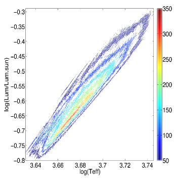
Figure 1: Degeneracy, i.e. number of model solutions, for 0.8 M_⊙ stars for a bin in Teff and L of 1000. The red areas correspond to regions of the HRD where we can find the highest degeneracy of 0.8 M_⊙ stellar model solutions.

3 Application to CG Cyg B

In order to illustrate our ANN’s capability for the identification of stellar model solutions we require a star with a mass similar to the one of the models used to train our tool. The eclipsing binary CG Cyg is located well within the solar vicinity (Popper, 1998). This constrains its component’s age, initial helium and metal abundances, well within the range of modelling parameters used to train our ANN. Moreover, the fact that CG Cyg’s lower mass component is a 0.810$\pm$0.013M_⊙ star (Popper, 1994), makes it a suitable target for our ANN.

Light curve analysis and I_c-band measurements allowed Hillenbrand and White (2004) to estimate CG Cyg B’s effective temperature (log(T${}_{eff})$=3.674$\pm$0.006) and luminosity (log(L/L_⊙)= -0.510$\pm$0.030). Taking into account these global stellar properties, our ANN identified 75412 sets of modelling parameters which reproduce, within the given uncertainties, CG Cyg B’s position in the HRD. These are shown in Fig.2a. Note that no model reproduces CG Cyg B’s exact position in the HRD. Yet, this is already expected since this star is lightly more massive than 0.8M_⊙.

The full range of possible modelling parameters is shown at Table 2. This shows that CG Cyg B admits almost all possible values for the initial helium and metal abundances (Figs. 2b and c). However, as seen in Fig.2f, these parameters are strongly correlated, presenting a linear correlation coefficient r=0.909 (corresponding to a false alarm probability smaller than 0.1%). Indeed, a linear fit to the model solutions gives:

$$Z=-0.0275+0.1736Y,$$ (1)

with a r.m.s.$\approx$0.0016. Figure 2f shows that, in most cases, the model’s initial helium and metal abundances are not in agreement with what is expected from a helium to metal enrichment ratio $\Delta$Y/$\Delta$Z=2, which takes into account the solar helium to metal proportion (Casagrande et al., 2007). Knowledge on the star’s metallicity would be valuable to test this enrichment ratio. Figure 2h shows that there is some degree of correlation between the model’s age and its chemical composition. The best fit to the data corresponds to:

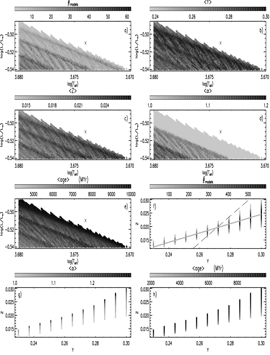
Figure 2: a) Number of model solutions for CG Cyg B (100 bins in log(T_eff) and log(L/L_⊙)). b) Average initial helium abundance for the same bin size. c) Average metallicity for the same bin size. d) Average mixing length for the same bins. e) Average age for the same bin size. The crosses corresponds to CG Cyg B’s exact position in the HRD. f) Number of model solutions for CG Cyg B (0.07 bin size in Y and 0.022 in Z). The solid grey line corresponds to the best linear fit to the model’s initial helium and metal abundances. The dashed line corresponds to a helium to metal enrichment ratio $\Delta$Y/$\Delta$Z=2. g) Average mixing-length parameter for different initial helium and metal abundances for the same bins. h) Average age for different initial helium and metal abundances of the same bin size.

Table 2: Range of modelling parameters for CG Cyg B.

Y		Z		$\alpha$		age (MYr)
min	max	min	max	min	max	min	max
0.23	0.30	0.01196	0.03	1.0	1.3	1850.754	10000.

$$age=3.46\times 10^{4}-1.527\times 10^{5}Y$$

$$+7.653\times 10^{5}Z~{}(MYr),$$ (2)

with a r.m.s.$\approx$902. In average, the model solutions seem to be older than the Sun (Fig.2e). This is reinforced by the fact, in the bin size that we have selected, the age standard deviation of the best models (i.e. those that better reproduce CG Cyg’s position in the HRD) is 1000MYr. Likewise, $\alpha$ is correlated with the model’s chemical composition (Figure 2g), with the best fit:

$$\alpha=1.537-3.462Y+22.927Z,$$ (3)

with a r.m.s.$\approx$0.055. Notice that every possible model has a mixing length smaller than 1.3 (Table 2 and Figs. 2d and g). This means the CG Cyg B’s $\alpha$ is clearly smaller than the solar value. Lastennet and Valls-Gabaud (2002) found no isochrone that could fit CG Cyg B’s position in the HR diagram, claiming that this star was far too cold. Yet, they assumed a solar mixing-length parameter. A lower mixing-length parameter (like the ones reported here) shifts the isochrones towards smaller effective temperatures.

Note that CG Cyg B is slightly more massive than the models used here. Thus it is important to assess the impact that this mass difference can have on the parameter estimation. Studies of main sequence stars such as the components of the UV Psc binary (Lastennet et al., 2003) or sub giants like $\beta$ Hyd and evolutionary models (Fernandes and Monteiro, 2003; Pinheiro and Fernandes, 2010) can provide us useful hints. In comparison with 0.80M_⊙ models, higher mass evolutionary tracks are shifted towards higher effective temperatures and luminosities. Moreover 0.81M_⊙ stars evolve faster. Therefore, CG Cyg B’s age should be slightly smaller than our models’ predictions. The models computed by Lastennet et al. (2003) and Pinheiro and Fernandes (2010) can be used to estimate the mixing-length’s mass dependence. Roughly speaking, the mixing-length’s mass dependence $\Delta$$\alpha$/$\Delta$M should be around -4, i.e. our models overestimate CG Cyg B’s mixing length parameter by a factor close to 0.04. Thus reinforcing furthermore our conclusions regarding this parameter. The same models can be used to derive a similar $\Delta$Y/$\Delta$M ratio. For instance, the overlap between Pinheiro & Fernandes’s evolutionary tracks of 0.90M_⊙ Y=0.29 and 0.92M_⊙ Y=0.25 stars indicates that our models overestimate CG Cyg B’s helium abundance by a factor 0.005. Lastennet et al.’s models hint a similar result. Finally, the same reasoning applied to the metalicity gives a $\Delta$Z/$\Delta$M ratio around -0.1, i.e. an 0.001 overestimation of CG Cyg B’s metalicity. This is close to what we obtain if we applied our helium overestimation to equation 1.

4 Conclusions

The strong correlation observed between the initial helium and metal abundances of CG Cyg B’s 0.80M_⊙ model solutions is similar to the one that can be seen in the analysis of UV Psc by Lastennet et al. (2003). Yet, no numerical relationship is explicitly given there. Moreover, we observe a correlation between the model’s chemical composition (Y & Z) and both their age and mixing-length parameter. Finally notice that for all possible models, the later parameter ($\alpha$) is smaller than the solar value. This could explain why for binary stars like CG Cyg, isochrones fail to fit, at the same time, both component’s position in the HRD.

Generally, we can constrain furthermore the modelling parameters of a given star by taking into account direct [Fe/X] observations and/or astreoseismic data. In the particular case of CG Cyg, we can simultaneously analyse both components (which should have the same age, initial helium and metal abundance). That leaves us with 5 unknown parameters (Y, Z, age, $\alpha_{A}$, $\alpha_{B}$) against 6 known global properties: M_A, T_effA, L_A, M_B, T_effB, L_B. Yet, this is not the scope of the present work. Indeed this work aims to show the adequacy of ANNs for the identification of modelling parameters which reproduce known global stellar properties and, consequently, their usefulness for analysing the degeneracy of stellar model solutions.

In this work we applied an ANN in order to perform a regression between the 4 parameters that we are searching and the two observables. The way our ANN is implemented ensures the reliability of this regression. Also notice that by treating the modelling parameters as free, we do not have the risk of suffering the consequences of assuming the wrong values. Additionally, once the ANN has been trained, our tool is able to identify the model solutions faster than approaches such as PSwarm (Fernandes et al., 2011) which, at each iteration, require the computation of an additional stellar models. This is particularly important in situations where a large number of stars have to be analysed. Likewise, our method’s accuracy in helium determination is competitive in relation to methods based on grid interpolations (Casagrande et al., 2007) On the other hand, the tool presented here is useful for the study of the degeneracy of stellar model solutions. Generally, only a small amount of solutions are evaluated (e.g. Fernandes and Monteiro, 2003), while here we have access to a large range of model solutions, allowing to analyse the degeneracy of model solutions problem as a whole.

Having shown the suitability of our method, we plan to apply our ANN to a larger sample of stars. This includes not only individual stars (for which their metal abundance may be known or not), binary stars and stellar populations, in particularly in clusters. This will allow studies on the chemical evolution of galaxies. Yet, in order to do so our Neural Network has to be trained using other stellar masses. The choice of the mass intervals needs to take into account the impact that this choice will have on the determination of stellar parameters. That will be slightly different for different regions of the HRD. In any case, a reasoning scheme similar to the one done here for CG Cyg B will be valuable.

In the future we plan to implement models with different masses in the web-based tool, i.e. using the mass as an additional output parameter The final result will be a tool that accepts txt files as inputs, trains and validates the ANN and produces outputs (both in text format and graphical form).

As a final remark we should remind that, like all works relying on the use of stellar evolutionary models, our ANN is limited by the set of models used to train it. This stresses the importance of using the right physical ingredients and assumptions.

References

- Andreon et al. (2000) Andreon, S., Gargiulo, G., Longo, G., Tagliaferri, R., Capuano, N., 2000. MNRAS 319, 700–716.
- Bailer-Jones (2000) Bailer-Jones, C. A. L., 2000. A&A 357, 197–205.
- Bishop (1995) Bishop, C. M., 1995. Neural Networks for Pattern Recognition. Oxford, Clarendon.
- Böhm-Vitense (1958) Böhm-Vitense, E., 1958. Zeitschrift fur Astrophysik 46, 108–+.
- Casagrande et al. (2007) Casagrande, L., Flynn, C., Portinari, L., Girardi, L., Jimenez, R., 2007. MNRAS 382, 1516–1540.
- Cassisi (2005) Cassisi, S., 2005. arXiv:astro-ph/0506161.
- Catelan (2007) Catelan, M., 2007. Structure and Evolution of Low-Mass Stars: An Overview and Some Open Problems. In: Graduate School in Astronomy: XI Special Courses at the National Observatory of Rio de Janeiro (XI CCE). Vol. 930 of American Institute of Physics Conference Series. pp. 39–90.
- Cunha et al. (2003) Cunha, M. S., Fernandes, J. M. M. B., Monteiro, M. J. P. F. G., 2003. MNRAS 343, 831–838.
- Demuth et al. (2008) Demuth, H., Beale, M., Hagan, M., 2008. Neural network toolbox 6. (The MathWorks).
- Duda et al. (2001) Duda, R., Hart, P., Stork, D., 2001. Pattern Classification. Wiley.
- Fernandes and Monteiro (2003) Fernandes, J., Monteiro, M. J. P. F. G., 2003. A&A 399, 243–251.
- Fernandes et al. (2011) Fernandes, J. M., Vaz, A. I. F., Vicente, L. N., 2011. A&A 532, A20.
- Haykin (1999) Haykin, S., 1999. Neural Networks. Prentice-Hall (New York).
- Hillenbrand and White (2004) Hillenbrand, L. A., White, R. J., 2004. ApJ 604, 741–757.
- Johnson et al. (2007) Johnson, J. A., Butler, R. P., Marcy, G. W., Fischer, D. A., Vogt, S. S., Wright, J. T., Peek, K. M. G., 2007. ApJ 670, 833–840.
- Lastennet et al. (2003) Lastennet, E., Fernandes, J., Valls-Gabaud, D., Oblak, E., 2003. A&A 409, 611–618.
- Lastennet and Valls-Gabaud (2002) Lastennet, E., Valls-Gabaud, D., 2002. A&A 396, 551–580.
- Mitchell (1997) Mitchell, T. M., 1997. Machine learning. McGraw Hill, New York.
- Morel (1997) Morel, P., 1997. A&AS 124, 597–614.
- Pinheiro and Fernandes (2010) Pinheiro, F. J. G., Fernandes, J. M., 2010. Ap&SS 328, 73–78.
- Popper (1994) Popper, D. M., 1994. AJ 108, 1091–1100.
- Popper (1998) Popper, D. M., 1998. PASP 110, 919–922.
- Stergiou and Siganos (1996) Stergiou, C., Siganos, D., 1996. Surprise96 4, www.doc.ic.ac.uk/~nd/surprise96/journal/vol4/cs11/ report.html.
- Tagliaferri et al. (2003) Tagliaferri, R., Longo, G., Incoronato, A., 2003. Special issue: Neural network analysis of complex scientific data: Astronomy and geosciences. Vol. 16 (Issue 3-4) of Neural networks. Elsevier Science Ltd.