Radiative Transfer and Radiative driving of Outflows in AGN and Starbursts

Abstract

To facilitate the study of black hole fueling, star formation, and feedback in galaxies, we outline a method for treating the radial forces on interstellar gas due to absorption of photons by dust grains. The method gives the correct behavior in all of the relevant limits (dominated by the central point source; dominated by the distributed isotropic source; optically thin; optically thick to UV/optical; optically thick to IR) and reasonably interpolates between the limits when necessary. The method is explicitly energy conserving so that UV/optical photons that are absorbed are not lost, but are rather redistributed to the IR where they may scatter out of the galaxy. We implement the radiative transfer algorithm in a two-dimensional hydrodynamical code designed to study feedback processes in the context of early-type galaxies. We find that the dynamics and final state of simulations are measurably but only moderately affected by radiative forces on dust, even when assumptions about the dust-to-gas ratio are varied from zero to a value appropriate for the Milky Way. In simulations with high gas densities designed to mimic ULIRGs with a star formation rate of several hundred solar masses per year, dust makes a more substantial contribution to the dynamics and outcome of the simulation. We find that, despite the large opacity of dust to UV radiation, the momentum input to the flow from radiation very rarely exceeds L/c due to two factors: the low opacity of dust to the re-radiated IR and the tendency for dust to be destroyed by sputtering in hot gas environments. We also develop a simplification of our radiative transfer algorithm that respects the essential physics but is much easier to implement and requires a fraction of the computational cost.

1 Introduction

Supermassive black holes (SMBHs) are thought to inhabit the central regions of nearly all massive galaxies and have properties well-correlated with those of their host galaxies (Gebhardt et al., 2000; Ferrarese & Merritt, 2000; Tremaine et al., 2002; Novak et al., 2006; Gültekin et al., 2009). The direction of the causal link between SMBH and host galaxy properties remains unclear, but the existence of such a correlation implies an intimate connection between the physics of SMBH growth and galaxy formation, spanning a factor of at least $10^{4}$ in length scale from $\sim 1\,\hbox{pc}$ to $\sim 10\,\hbox{kpc}$.

Quasars came to astronomers’ attention due to their enormous electromagnetic output. Bright active galactic nuclei (AGN) emit as much as $10^{47}\,\hbox{erg}\,\hbox{s}^{-1}$ over the electromagnetic spectrum (Woo & Urry, 2002; Kollmeier et al., 2006). A significant amount of careful work has been performed to study the physical effects of this extraordinary outpouring of electromagnetic energy and momentum on the material in the immediate vicinity of the AGN (e.g. Proga et al., 2000, 2008; Kurosawa & Proga, 2009; Park & Ricotti, 2011, 2012). As a result we are beginning to understand the radiation driven broad-line winds emerging from discs around the central SMBHs. However, relatively little work has been done regarding the radiative effects on the surrounding galaxy.

There has been intense theoretical interest in the ability of AGN to affect the star formation histories and observed colors of galaxies (e.g. Croton et al., 2006; Schawinski et al., 2007). The relationships between star formation, and AGN activity, galaxy mergers, and secular processes have turned out to be complex and the parameter space is not yet fully mapped. What is clear is that gas added to the central regions of galaxies will induce a central star burst and an AGN flare-up, but the triggering mechanism remains uncertain.

Although the use of numerical simulations to study the interactions between black holes and galaxies has a long history (e.g. Binney & Tabor, 1995; Ciotti & Ostriker, 1997), work by Di Matteo et al. (2005) and Springel et al. (2005) set off an explosion of theoretical work. They studied the simplest reasonable fully specified model of black hole fueling and AGN feedback in the context of a major mergers of gas-rich spiral galaxies and found that the AGN has a profound effect on the gas dynamics and star formation history in the merger remnant.

During the combined AGN/starburst phase, analytical investigations by Thompson et al. (2005) and Murray et al. (2005) have shown the importance of radiative forces on dust. Subsequent numerical work (Debuhr et al., 2010; Debuhr et al., 2011, 2012) has verified that if the central $\simeq$ 100 pc of galaxies are assumed to have optical depths of 10 to 25 in the infrared, due to dust opacity, then radiative forces on dust have dramatic dynamical consequences in the context of merging galaxies.

As the investigations have become more detailed and accurate, it has become increasingly necessary to perform the radiative computations in a more rigorous fashion, carefully determining both the energy and momentum input into the ambient gas. It is the purpose of this paper to outline some of the principles and techniques that may be used for this task.

Our goal is to develop a numerical method to self-consistently solve the radiative transfer problem in galaxies in the presence of dust and radiation produced by stars and AGN. That is, we would like to solve for the specific intensity of the radiation field for a given distribution of radiation sources in the presence of scattering and absorbing media, and subsequently use the specific intensity to compute the forces on the scattering/absorbing media. Studies of SMBH fueling and AGN feedback performed to date have either ignored radiative effects or else assumed a particular form of the photon field which is then used to compute forces on the gas.

Although it would be ideal to obtain a perfect solution for the radiation field in all cases, we will settle for a method that gives the correct asymptotic behavior in all relevant limits and interpolates reasonably between the limits. It should respect global conservation laws for energy and momentum. It must not be overwhelmingly demanding in terms of algorithmic complexity or computational resources.

The paper is organized as follows: In Section 2 we summarize previous theoretical work on AGN feedback as well as some recent observational results. In Section 3 we discuss the radiative transport equation in the context of the present problem. We describe the physics behind it, its most important properties, and the different approaches that can be used for the numerical solution. In Section 4 we describe the physics implemented in a two-dimensional hydrodynamical code designed to study black hole fueling and radiative feedback from AGN and star formation in the context of early-type galaxies. In Section 5 we present the main results of the simulations. Finally in Section 6 we summarize our conclusions.

2 Previous Work

It has long been known that the bulk of the matter that enters black holes over the history of the universe does so via radiatively efficient accretion (Soltan, 1982; Yu & Tremaine, 2002). The resulting photons are the clearest observational indication that SMBH accretion is taking place.

There is a prodigious amount of energy and momentum available during Eddington-limited bursts consequent to accretion, certainly enough to have a profound effect on the structure and dynamics of the interstellar medium.

2.1 Mechanical feedback

Many AGN are observed to have broad absorption lines indicating strong outflows. Several physical processes operating near the SMBH could plausibly launch these winds (e.g. Proga et al., 2000) and they go under the heading of mechanical feedback regardless of the details of their origin (Ostriker et al., 2010). They are thought to be somewhat collimated and are thus only observed in 1/4 to 1/2 of all bright AGN. Recently, quantitative estimates of the kinetic energy in these outflows have become available (Moe et al., 2009; Arav et al., 2012) and indicate that they contain 0.1-1% of the energy in the radiative component of the AGN output.

This mechanical energy can couple to the ISM much more efficiently than the AGN photons, making this an attractive mechanism for AGN feedback. However, there are significant observational uncertainties in these kinetic wind energy estimates, the studies have only been carried out for a few objects, and there is no global constraint analogous to the Soltan (1982) argument that allows an estimate of the global mean efficiency of energy conversion to kinetic winds in AGN. If the Moe et al. (2009) estimate of the kinetic luminosity is correct and we assume all of the mechanical energy and momentum is effectively deposited into the ISM, then mechanical feedback will dominate over radiative feedback for column densities less than $10^{-21}$ to $10^{-22}\,\hbox{g}\,\hbox{cm}^{-2}$.

2.1.1 Simulations of mechanical feedback

Many groups have carried out substantially similar studies of AGN feedback in the context of galaxy mergers where the black hole accretion rate is given by the smaller of the estimated Bondi rate and the Eddington rate, while the AGN feedback is assumed to be purely thermal energy injected in the vicinity of the black hole. This is the basic model developed by Di Matteo et al. (2005) and Springel et al. (2005) and applied extensively to compare with observations of the quasar luminosity function, galaxy colors, and more (e.g. Hopkins et al., 2005, 2006, 2008). The same basic model was also used by Johansson et al. (2009), and all authors found that AGN feedback has a dramatic effect on galaxies provided that 5% of the bolometric AGN output is transformed into thermal energy within 100 pc of the black hole by mechanical winds operating on smaller scales.

However, observations of gas dynamics near AGN have indicated that the actual efficiencies are a factor of 5 to 50 smaller than the value usually used in many of these simulations (Moe et al., 2009; Arav et al., 2012). Booth & Schaye (2009) and Choi et al. (2012) have carried out careful studies of the underlying numerical and physical assumptions that go into this feedback model, the latter paper finding that including the radial momentum of the AGN ejecta in the calculation dramatically increases the efficiency of mechanical feedback.

Dubois et al. (2010) developed a model of AGN involving anisotropic injection of kinetic energy on scales similar to the resolution of the simulation. They implemented this model in the adaptive-mesh-refinement code RAMSES (Teyssier, 2002) and studied the implications of this feedback model on the properties of black holes and galaxy clusters in cosmological simulations a resolution of approximately one kiloparsec.

Gaspari et al. (2012) performed simulations of the evolution of the ISM of an elliptical galaxy in the presence of AGN feedback similar to that of Dubois et al. (2010). In terms of the galaxy model and the treatment of stellar evolution and mass loss, the simulations are substantially similar to those presented here. The differences include the fact that the Gaspari et al. (2012) simulations are three dimensional rather than two dimensional, have much lower spatial resolution ($\simeq 150\,\hbox{pc}$ rather than $0.25\,\hbox{pc}$, and include feedback only via anisotropic injection of kinetic energy, rather than the more comprehensive feedback model presented here. Gaspari et al. (2012) found that mechanical feedback efficiencies in the range of those observed by Moe et al. (2009) and Arav et al. (2012) were sufficient to limit black hole growth, balance atomic cooling, and lead to observationally reasonable gas density and temperature profiles, in substantial agreement with the conclusions of Novak et al. (2011), Ciotti et al. (2010), and other studies.

The observational studies of Moe et al. (2009) and Arav et al. (2012) indicate that this form of mechanical feedback only uses a small fraction of the available energy. This motivates the study of other forms of radiative feedback.

2.2 Radiative momentum feedback

It is well-known that the photons couple to the ISM weakly if only the small Thompson cross section is considered (e.g. Ciotti & Ostriker, 2001). Of the momentum available, only a fraction $\tau_{\rm ES}$ (the optical depth to electron scattering) couples to the ISM, while there is no additional energy transfer to the gas in the case of pure Thompson scattering of photons having $E\ll 1\,\hbox{MeV}$. Only a small fraction of AGN are known to be optically thick to Compton scattering, although studies of the X-ray background indicate that Compton-thick AGN may be common at high redshift (Daddi et al., 2007). X-rays couple more strongly than lower energy photons (Sazonov et al., 2005) due to both inverse Compton effects and coupling with resonant metal lines. Nevertheless, the $M_{\rm BH}--\sigma$ relation (Gebhardt et al., 2000; Ferrarese & Merritt, 2000) has been construed as evidence that black holes regulate their growth via momentum-driven winds (King, 2003).

Radiation also couples to the ISM through scattering/absorption by dust grains as well as atomic resonance lines. The cross section for dust absorption in the UV for solar metallicity gas with a dust/gas ratio typical of the Milky Way can be 3500 times the electron scattering cross section (Draine, 2003), while that for resonance lines can be the same or greater (Proga et al., 2000; Sazonov et al., 2005). This means that radiative feedback due to line or dust absorption can provide more energy and momentum than mechanical feedback for column densities as low as $10^{-18}$ to $10^{-19}\,\hbox{g}\,\hbox{cm}^{-2}$.

The potential importance of radiative momentum feedback has been known for some time (Haehnelt, 1995; Ciotti & Ostriker, 2007, hereafter C07), but the particular importance of dust in the context of AGN and starbursts was pointed out by Murray et al. (2005) and Thompson et al. (2005). Simulations by Debuhr et al. (2010); Debuhr et al. (2011, 2012) model the effect of radiation pressure acting on dust at radii large compared to the black hole but small compared to the galaxy. Note that while the physical process mediating the interaction between the SMBH and the ISM is different from the mechanical model of Di Matteo et al. (2005), the photon momentum is converted to hydrodynamic motion on scales smaller than the resolution of the simulation ($\sim 100$ pc).

2.2.1 Simulations of radiative feedback

Sazonov et al. (2005) investigated the important effects of X-ray heating and Ciotti & Ostriker and collaborators have incorporated all of the standard electromagnetic processes into their one-dimensional treatments of the cooling flow initiated AGN outbursts (C07; Ciotti et al., 2009, 2010; Ciotti & Ostriker, 2012). These investigations represent a different viewpoint from the “conventional” view that AGN are associated with mergers. Here, the AGN activity attributed to the reprocessing of gas lost by the evolving stellar population of an isolated and “passively” evolving early-type galaxy. In section 2.5 we comment on recent observations that bear on this point. Recently Hensley et al. (2012) have added an improved treatment of dust creation and destruction as well as a calculation of the dust temperature to these one-dimensional models.

Feedback in the Debuhr et al. simulations is implemented via a force on the gas assuming that there is a fixed optical depth to IR photon scattering by dust at all times ($\tau\simeq 10$). No self-consistent solution for the radiation field is sought. The radiative force is applied over one resolution element near the black hole, so, although the physical model posits a radiative origin for the computed forces, in implementation their algorithm bears some resemblance to mechanical feedback schemes in that it is purely local and the photons do not exert forces over macroscopic distances in the simulation.

Novak et al. (2011) used the same physical model described in Sazonov et al. (2005) and C07 (with the exception of the radiative forces on dust) to run two-dimensional simulations of SMBH fueling and AGN feedback. The present work extends Novak et al. (2011) to include radiative forces on dust grains. We seek to carry out the radiative transfer calculation due to photon absorption and scattering by dust in a self-consistent fashion.

Hambrick et al. (2011) and Kim et al. (2011) carried out simulations of black hole fueling and AGN feedback during galaxy mergers and found that the addition of X-ray heating by the AGN allowed the black hole to regulate its own growth by keeping its immediate vicinity hot without necessarily heating the majority of the gas in the galaxy. Hambrick et al. (2011) used cosmological smoothed-particle-hydrodynamics (SPH) simulations with a simple treatment of X-ray photons from the AGN. Kim et al. (2011) performed adaptive-mesh simulations of galaxy mergers reaching a resolution of 15 pc. The simulations tracked mechanical feedback in the form of a collimated outflow generated near the black hole as well as radiative feedback in the form of X-rays generated by the AGN. The X-rays transferred energy and momentum to the surrounding gas, via by a three-dimensional Monte Carlo ray tracing algorithm.

2.3 Angular momentum transport

Several efforts have focused on understanding angular momentum transport in the absence of feedback. This eases one of the severe computational constraints in the problem, since it is feedback that generates high gas temperatures and large gas velocities, necessitating very short simulation time steps and therefore very large computational costs per simulation. Levine et al. (2008) used adaptive-mesh cosmological simulations to examine gas transport from cosmological scales to $\simeq$ 1 pc from the black hole. Hopkins & Quataert (2010) carried out nested zoom-in simulations of the central regions of a galaxy undergoing a major merger. Both groups concluded that the mutual gravitational torques exerted by clumps of gas were sufficient to transfer angular momentum away from the central regions and permit accretion, and that the scale-free nature of gravity allowed the process to proceed in a nested fashion through all scales to the presumed black hole accretion disk. It is very attractive to split the problem of black hole fueling and AGN feedback into a fueling part and a feedback part. However, one would expect gas clumpiness to be dramatically reduced if AGN are able to heat the ISM significantly, which would in turn shut down the angular momentum transfer process that these authors envision. If the gas clumps are shielded from the AGN photons by a central dusty torus, or if the clumps of gas are self-shielding, then the process may continue to operate in spite of AGN feedback.

2.4 Sub-parsec simulations

As high-resolution simulation efforts that resolve the Bondi radius become more common, technical details of the numerical solution become important. Barai et al. (2011) have performed a detailed study of the numerical and physical aspects of simulating Bondi accretion using SPH in the presence of heating by a central black hole over scales of 0.1 to 200 pc. They conclude that typical formulations of the artificial viscosity term typically used in SPH can cause excessive heating near the inner boundary of the simulation.

Dorodnitsyn et al. (2012) have studied the radiation hydrodynamics of the inner few parsecs of galaxies in the presence of dust in the the flux-limited diffusion approximation. They show that the dusty torus around AGN is plausibly supported by radiation pressure on dust in an outflowing wind. They are interested in smaller physical scales than presently concern us, and they are only interested in the limit of large optical depths to scattering by dust in the infrared. However, there is significant overlap in the basic physics between their work and the present paper.

2.5 Observations concerning mergers, star formation, and AGN

The observational situation regarding the links between black hole growth, star formation, and mergers has been somewhat confused, although it seems that a preponderance of evidence is now indicating that, although mergers may trigger AGN, the majority of AGN are not triggered by mergers.

Pierce et al. (2007) used a combination of X-ray data, space-based optical data, and ground-based optical data, all part of the AEGIS survey (Davis et al., 2007), to conclude that X-ray selected AGN preferentially reside in early-type galaxies and that although the X-ray selected AGN were more often members of close pairs, the companion was usually undisturbed. This was interpreted as evidence against interactions triggering AGN.

Using Sloan Digital Sky Survey data, Cisternas et al. (2011) found a strong correlation between close galaxy pairs and galactic star formation, but no correlation between between close pairs and AGN activity. Schawinski et al. (2010) conducted a similar study and found superficially similar correlations, but based on their results connecting galaxy color to stellar population age (Schawinski et al., 2007) argued that the lack of AGN with close companions was due to a delay between the final merger and the onset of AGN activity.

Ellison et al. (2011) have found that close pairs tend to have AGN activity, but that AGN do not have an elevated close companion rate. They argue that mergers do indeed cause AGN activity, but that the majority of AGN are caused by other, presumably secular processes.

Diamond-Stanic & Rieke (2012) found that AGN activity is correlated with nuclear star formation (within $\sim$100 pc), but not with global star formation on kiloparsec scales.

Rosario et al. (2011) used space-based optical and x-ray data taken as part of the CANDELS survey (Grogin et al., 2011) to conclude that there is little difference between X-ray selected AGN and quiescent galaxies in terms of colors and stellar populations out to a redshift of three, arguing against a scenario where a significant fraction of AGN are triggered by mergers. As part of the same survey, Kocevski et al. (2012) concluded that X-ray selected AGN are not morphologically different from a mass-matched sample of quiescent galaxies.

3 The Radiative Transfer Equation

In this section, we develop a method of treating the radiative forces forces on the ISM gas in a galaxy. Our goal is to arrive at an algorithm that gives the correct behavior in the many asymptotic limits required by the physical problem at hand.

First we discuss the astrophysical requirements that motivate some of the choices we have made in defining the method. In the present work we are primarily concerned with radiative forces on dust grains, but the method works for any source of isotropic scattering or absorption opacity.

More precisely, we derive three related algorithms for solving the radiative transfer equation. All of them arise from developing a set of moment equations for the specific intensity. For each method, we derive set of differential equations, the solution of which give the mean intensity and net flux of the photon field.

The first method (Section 3.2) gives a boundary-value problem where the physical content of the set of differential equations is quite transparent. However, closing the set of differential equations in this method requires us to rely rather heavily on our physical intuition about the solution.

The second method (Appendix A) also gives boundary-value problem and is more aesthetically pleasing in a formal mathematical sense because the closure relation is derived along with the set of differential equations—it does not require a physically motivated guess. The cost an additional differential equation to solve and the fact that the physical content of the equations is somewhat more opaque compared to the first method.

The third method (Appendix B) is an attempt to capture the essential behavior of the system while reformulating it as an initial value problem. The reason for this is that it is vastly simpler to efficiently and robustly obtain the numerical solution to an initial value problem.

Note that in this work we use the first of these three methods and present the other two for reference and for future work. All three of the algorithms are self-consistent in the sense that we first solve for the photon field and then learn from this solution whether the radiation field is nearly isotropic (like the interior of a star) or highly directed (like a point source), whether the energy is carried by UV, Optical, or IR photons, and so on. We do not assume a priori that the system is in any particular asymptotic limit of the radiative transfer equation.

We neglect angular force terms and although we use spherical symmetry to derive the differential equations, we argue in Section 3.2.1 that the method can be used with good results even in the case where the system is not spherically symmetric.

3.1 Astrophysical preliminaries

Over their lifetimes, galaxies explore essentially all of the asymptotic limits of the radiative transfer equation. Most of the time, most lines of sight are optically thin to radiation and the central SMBH is not accreting significantly, so the radiation field within the galaxy is nearly isotropic and produced by a spatially distributed source (the stars themselves). However, most galaxies undergo brief periods of intense SMBH accretion, during which time the radiation field is dominated by the central point source and is not isotropic. During these times, most lines of sight remain optically thin, but a few lines of sight pass through the central dusty torus which is highly optically thick to UV/optical photons. Furthermore, many galaxies probably have spent time in a LIRG/ULIRG state involving intense bursts of star formation with a nearly spherical, highly optically thick ISM in the central regions. In this case, the radiation field may be sourced primarily by the central point source or the distributed stars, and in either case repeated scattering and absorption of UV and optical photons make the radiation field tend toward isotropy. Overall, the galaxy does not spend much time in this highly optically thick state, but interesting and important things are happening during that time.

It is crucial to note here that all of the energy absorbed in the UV/optical bands must be re-emitted as long-wavelength photons, because to neglect the re-emission is to ignore energy and momentum conservation. In particular, ULIRGs are optically thick even to electron scattering over essentially all lines of sight, so the diffusion of the reprocessed IR photons can have a significant impact on the state of the gas in the galaxy (Murray et al., 2005; Thompson et al., 2005).

In the optically thin case, the radiation field is highly directed in the region where the point source dominates. This region always exists at sufficiently small radii for a true point source. If and when the stellar light starts to dominate the radiation field, it becomes nearly isotropic for radii within the region that is producing the bulk of the photons. For significantly larger radii, the radiation field again becomes directed as the photons emerge from the galaxy on nearly radial paths heading toward infinity.

If the ISM is optically thick to scattering, the radiation field quickly becomes isotropic even if the photons come from a central point source. In the UV and optical part of the spectrum, the opacities to scattering and absorption due to dust are of the same order of magnitude. Typically the scattering opacity is less than the absorption opacity (Draine, 2003), in which case the primary effect of scattering is to make the radiation field tend toward isotropy, rather than trapping photons so that they diffuse out of the galaxy. Therefore in adopting a closure relation we will assume that the radiation field becomes nearly isotropic (although still maintaining a net outward flux) when the optical depth to scattering or absorption is greater than unity. If the scattering opacity is much smaller than the absorption opacity, this is incorrect: a highly directed radiation field from a point source is always highly directed even after many (absorption) optical depths. However, for realistic dust properties the scattering and absorption opacities are of the same order of magnitude.

If a UV or optical photon is absorbed rather than scattered, then the energy is reprocessed into the IR, but the energy is lost to the UV. Thus absorption will not tend to change the angular character of the radiation field (directed versus nearly isotropic). However, for declining density distributions, the column density $\int\rho\kappa dr$ is dominated by what is occurring at small radii, whereas the energy injected by stars, $\int\epsilon 4\pi r^{2}\,dr$ (where $\epsilon$ is the emissivity for stellar photons), is dominated by what happens at large radii unless the stellar distribution falls off as $r^{-3}$ or faster. Therefore, even if absorption dominates over scattering (as it does in the UV), if the ISM is optically thick, the central point source will quickly be diminished compared to the radiation produced by stars.

Radiative transfer is difficult in general, in part because of the high dimensionality of the problem. The quantities of interest are functions of spatial position, photon propagation direction, frequency, and time, giving seven dimensions in total. Furthermore, the solution is subject to non-local effects: photons tend to leave a system via optically thin “windows” if they are available. A nearly spherical gas cloud with optical depth $\tau$ along most lines of sight and a few clear lines of sight comprising solid angle $\Omega$ will trap photons roughly as though it had effective optical depth $\tau_{\rm eff}=\min(\tau,\Omega/4\pi)$. That is, in order to effectively trap photons within an optically thick cloud, it is necessary to have a covering fraction of order $1/\tau$ or else the photons will leak out of optically thin “holes.”

3.2 Mathematical treatment

Using the physical insight provided by the discussion in Section 3.1, we now seek a mathematical formulation of the problem that is not overwhelmingly computationally intensive and is correct (or nearly so) in each of the identified limits (optically thin/thick, radiation field nearly isotropic/highly directed, dominated by distributed source/point source, and gas distribution nearly spherical/highly non-spherical).

We must distinguish the variables specifying the photon propagation direction from spatial position; to this end we stipulate that $\tilde{\theta}$ and $\tilde{\phi}$ refer to spatial position while $\theta$ and $\phi$ refer to photon propagation direction. Without loss of generality, in the case of isotropic scattering, as we consider in our treatment, the frequency-integrated equation of radiative transfer is

$$\frac{dI(\mu,\phi)}{ds}=-\rho(\kappa_{a}+\kappa_{s})I+\rho\kappa_{s}J+\epsilon\,,$$ (1)

where $s$ is the distance along the arbitrary direction of the ray, $\mu=\cos\theta$, $\theta$ is the angle between the ray propagation direction and the $z$ axis, $\phi$ is the azimuthal angle, $I\equiv dE/dt\,d\Omega\,dA$ is the specific intensity, $J\equiv\int I\,d\mu\,d\phi/4\pi$ is the mean intensity, $\rho$ is the gas density, $\kappa_{a}$ is the cross section for absorption per unit mass, $\kappa_{s}$ is the cross section for scattering per unit mass, and finally $\epsilon$ is the emissivity per unit solid angle (Chandrasekhar, 1960). All quantities are functions of spatial position and time, suppressed above for brevity.

If we further adopt spherical symmetry, i.e., all quantities are independent of spatial position $\tilde{\theta}$ and $\tilde{\phi}$, then eq. (1) becomes

$$\mu\frac{\partial I}{\partial r}+\frac{1-\mu^{2}}{r}\frac{\partial I}{\partial\mu}=-\rho(\kappa_{a}+\kappa_{s})I+\kappa_{s}J+\epsilon\,.$$ (2)

Here we seek a solution to this equation by taking moments in $\mu$ and integrating away the dependence of the photon field on propagation direction. The final ingredient is a physically reasonable closure relation to terminate the set of moment equations, to be discussed below.

Note that although we write the radiative transfer equation in spherical form, the numerical method we outline does not require spherical symmetry. The gas density, opacities, and photon field may vary as a function of $\tilde{\theta}$ and $\tilde{\phi}$. Further details including the method by which this is accomplished as well as advantages and disadvantages of our formulation are discussed in Section 3.2.1.

The considerations in Section 3.1 can be summarized by the ansatz that the specific intensity to be composed of three terms: one isotropic, one mildly anisotropic, and one highly directed:

$$I=A+B\mu+D\delta(\mu-1)\,,$$ (3)

where $\delta$ is the Dirac delta function and the three coefficients (which are functions of time and radial coordinate) are adjusted as described below. Incorporating the last term (with $D>0$) permits us to allow for phases when the central point-like quasar dominates the radiation field and to correctly treat the photon field far outside of the galaxy where the specific intensity resembles that of a point source. Note that if we were to take $D=0$ in eq. (3), then we would arrive at the Eddington approximation, which is commonly adopted in stellar interiors. Taking eq. (3) as a generalization of the Eddington approximation allows us to interpolate smoothly between the limits of a central point source and an optically thick situation.

Taking moments in $\mu$ of the specific intensity to remove the explicit dependence on the ray propagation direction gives:

$$J\equiv\frac{1}{4\pi}\int_{0}^{2\pi}d\phi\int_{-1}^{1}I(\mu,\phi)\,d\mu=A+\frac{D}{4}\,,$$ (4)

$$F\equiv\int_{0}^{2\pi}d\phi\int_{-1}^{1}\mu\,I(\mu,\phi)\,d\mu=\frac{4\pi B}{3}+\pi D\,,$$ (5)

and

$$P\equiv\frac{1}{c}\int_{0}^{2\pi}d\phi\int_{-1}^{1}\mu^{2}I(\mu,\phi)\,d\mu=\frac{4\pi A}{3c}+\frac{\pi D}{c}\,,$$ (6)

where $J$ is the mean intensity, $F$ is the energy flux, and $P$ is the radiation pressure.

We must find some physically plausible way to decide whether the radiation field is nearly isotropic (in which case the standard Eddington closure relation $P=u/3$ applies, where $P$ is the radiation pressure and $u$ is the energy density) or highly directed (in which case the flux is simply related to the zeroth and second moments of the specific intensity).

To find the appropriate equations, we take two moments of eq. (2) in two different cases. First, when the radiation field is mildly anisotropic ($D=0$) with the closure relation $P=4\pi J/3c$, yielding the differential equations for the photon field in the classic Eddington approximation:

$$\frac{dL}{dr}=4\pi r^{2}(\dot{E}-4\pi\rho\kappa_{a}J)\,,$$ (7)

$$\frac{dJ}{dr}=-\frac{3\rho(\kappa_{a}+\kappa_{s})L}{16\pi^{2}r^{2}}\,.$$ (8)

Second, when the radiation field is highly directed ($A=B=0,D=1$) with the closure relation $P=4\pi J/c$, appropriate for a point source. In this case the equation for $dL/dr$ is the same and the equation for mean intensity becomes

$$\frac{dJ}{dr}=-\frac{2J}{r}-\frac{\rho(\kappa_{a}+\kappa_{s})L}{16\pi^{2}r^{2}}\,.$$ (9)

The first term on the right-hand side gives the expected $r^{-2}$ fall-off of the mean intensity if the radiation field is primarily directed (e.g. outside of the galaxy).

We combine equations eqs. (8) and (9) for $dJ/dr$ by introducing the variable $t$ that interpolates between the optically thin (radiation field like a point source) and optically thick (radiation field nearly isotropic) cases. This gives:

$$\frac{dL}{dr}=4\pi r^{2}(\dot{E}-4\pi\rho\kappa_{a}J)\,,$$ (10)

$$\frac{dJ}{dr}=-\frac{2Jt}{r}-\frac{(3-2t)\rho(\kappa_{a}+\kappa_{s})L}{16\pi^{2}r^{2}}\,,$$ (11)

where $t=0$ when the radiation field is nearly isotropic and $t=1$ when it is highly directed. In practice, we take $t$ as a function of position to be:

$$1-t(r)\equiv\frac{1}{1+e^{5(1-\tau_{\rm out})}+e^{5(1-\tau_{\rm in})}}\,,$$ (12)

where

$$\tau_{\rm in}(r)=\int_{0}^{r}\rho(\kappa_{a}+\kappa_{a})\,dr\,,$$ (13)

and

$$\tau_{\rm out}(r)=\int_{r}^{\infty}\rho(\kappa_{a}+\kappa_{a})\,dr\,.$$ (14)

Evaluating $t$ as $r$ becomes very large or very small gives $t=1$ at the inner boundary (near the AGN) and at the outer boundary (far from the galaxy). If the ISM is optically thick there will be some region in between where $t$ is nearly 0. This choice expresses our expectation about where the radiation field should be primarily directed versus primarily isotropic. The factors of five in eq. (12) are chosen to ensure that the value of $t$ switches from the optically thin limit to the optically thick limit fairly quickly near optical depths of unity. The transition effectively occurs between optical depths of 0.8 and 1.2.

Finally we specify the boundary conditions. As in the study of stellar interiors, our second order differential equation for $L(r)$ requires two boundary conditions, one at the center and one at the outer surface. Near the center of the simulation, the outgoing luminosity is only that provided by the central point source, the AGN. Far from the galaxy, the radiation field is expected to again look like a point source as scattering/absorption become negligible and all of the photons leave the galaxy. The two natural boundary conditions are then

$$L(r_{\rm min})=L_{\rm BH}\,,$$ (15)

and

$$J(r_{\rm max})=\frac{L(r_{\rm max})}{16\pi^{2}r_{\rm max}^{2}}\,.$$ (16)

The force on the gas in a computational cell is

$$\Delta f=\frac{L(r)d\tau dA}{4\pi r^{2}c}\,,$$ (17)

where $d\tau$ is the optical depth (scattering plus absorption) of a given cell and $dA$ is the area of the cell perpendicular to the radiation flux vector.

3.2.1 Comments on the spherical symmetry assumption

We are primarily interested in what happens to the ISM as a function of radius rather than angle. Angular effects are important and it is of crucial importance to break spherical symmetry so that hydrodynamic instabilities such as convection and the Rayleigh-Taylor instability can operate. However, we are concerned mainly with whether gas makes it to small radii (and accretes onto the black hole) or to large radius (and escapes the galaxy), not where on the sphere the gas enters the SMBH or leave the galaxy. Thus we neglect all angular radiative forces and formulate the radiative transfer as occurring exclusively along rays from the center of the galaxy.

Similar approximations have been used in numerical simulations of photon and neutrino transport in supernovae for some time (e.g. Brandt et al., 2011, and references therein). One approach is to spherically average the matter distribution, solve for the radiation field, and then calculate forces on matter via eq. (17). Another approach is to treat each ray as a separate problem, in which case all intensive quantities (gas density, emissivity of stellar photons, etc) are treated as though they obtained over the whole sphere.

We found that the first approach has dramatic failure modes where it wildly overestimates the outward radial forces on the gas in certain situations. As an example, consider an optically thick cloud covering a small solid angle in an otherwise optically thin medium. In reality, UV photons deposit momentum in a thin layer at the surface of the cloud, and the total momentum imparted to the cloud depends on the solid angle of the cloud. However, spherically averaging the matter distribution may result in the ISM becoming optically thin at the cloud radius, and the solution for the photon field will indicate that the UV flux is high throughout the cloud. In this case, essentially all of the dust grains in the cloud are able to absorb UV photons and the momentum imparted to the cloud will be wildly overestimated.

Instead, treating each ray as a completely independent problem has much better behavior in the sense that when the algorithm makes an error in computing the force on a particular gas cell, fractional error tends to be of order unity rather than orders of magnitude. In the previous example, this method gives the correct force exerted by UV photons. For the IR photons, the method assumes that they must traverse the cloud on their way out of the galaxy, while in reality they would leave the system via the optically thin ambient medium. Therefore the method makes a a fractional error of order the IR optical depth when computing the force.

One drawback of the latter approach is that if a particular ray (say, near the pole) has deficient star formation compared to the rest of the galaxy, then the forces exerted by the stellar photons will be anemic compared to the true solution, where stars from near the midplane emit photons that help push on gas near the poles. Therefore, we average source terms over a sphere before finding the solution to the radiative transfer equations on each ray.

Note that this method allows the radiation field to differ in an unlimited way from one ray to the next. This is expected for example in the UV where the scattering opacity is less than the absorption opacity, and the interior of an individual “cloud” along a line of sight can be shielded from the AGN UV luminosity. However, in the IR we consider the absorption opacity to be zero, and it no longer makes sense that the radiation field could differ substantially on adjacent rays. Therefore we also spherically average the IR source terms (in particular IR generated by absorption of UV or optical) before solving for the luminosity as a function of radius in the IR.

3.3 Numerical implementation

The numerical solution of the radiative transfer equation is complicated by the fact that one boundary condition is specified at $r_{\rm min}$ while the other is specified at $r_{\rm max}$ (note eqs. (15) and (16)). Thus, integration from either side requires a guess that must be refined. This is identical to the situation in treating the radiative transfer in stellar interiors. Conceptually, this is simply because we know the central luminosity, but we do know know the intensity of the radiation field near the center. If the scattering opacity is large, photons will build up in the galaxy forming a nearly isotropic radiation field until the gradient of the photon density is sufficient to drive photon diffusion out of the galaxy at the rate required to carry the specified luminosity.

In fact, the numerical solution to the radiative transfer equation in stellar interiors is considerably simpler than in the present problem because within stars, one can exploit the fact that the plasma is everywhere close to local thermodynamic equilibrium. The plasma is assumed to quickly thermalize any energy sources or sinks so that the plasma is well-described by a single temperature at any point. In galaxies, the photon field is not close the thermodynamic equilibrium and we must track energy as it is transferred from x-rays to UV photons and eventually to IR photons. Treating stellar interiors in an analogous way would mean tracking each energy band of photons separately as the star’s luminosity was transported through the plasma, from the primary MeV photons produced by fusion reactions, to the UV photons that eventually emerge from the photosphere.

To find the solution of eqs. (10) and (11) subject to the correct boundary conditions eqs. (15) and (16), the “shooting method” with Newton-Raphson iteration (Press et al., 1992) works well up to optical depths of a few. Beyond that, the absorbing gas acts as a very effective “screen” that hides conditions near the center of the simulation from those at the outer edge. This makes it very difficult to find the correct solution matching both boundary conditions at once. We would like to simulate AGN feedback in galaxies with gas surface density up to Compton-thick, implying an optical depth to dust absorption in the UV of several thousand. The shooting method is too unstable to use in this case.

It is true that given such a large optical depth, very little of the primary UV radiation escapes the galaxy; it comes out in the IR. However, it is incorrect to discard the primary UV radiation completely, or to immediately transfer it to the IR. While this would correctly give the emergent energy, the UV radiation can have a very large effect near the center of the galaxy before it is transferred to the IR. For for solar composition and dust/gas ratios, they can limit the accretion rate to $3\times 10^{-4}L_{\rm Edd}$.

At large optical depths, the more powerful “relaxation” iterative method (Press et al., 1992) is required to adjust the solution over the entire domain of integration while ensuring that the proper boundary conditions are met at both ends of the interval. Newton’s method is used to iterate over trial solutions to arrive at the solution to the differential equations, where the independent variables of the Newton iteration are taken to be the values of $L$ and $J$ at each spatial point. The method takes the coupling between variables at neighboring points into account, allowing the entire solution to be updated without overcompensating (which the shooting method is prone to do). Given a good initial guess for the iteration, the relaxation method finds a reasonably accurate solution even for very large optical depths. The initial guess is conveniently provided by the solution that pertained during the previous simulation time step.

Two additional numerical schemes are defined in appendicies. The method described in Appendix A allows one to avoid using the variable $t$ and its somewhat ad hoc definition in eq. (12) at a cost of one additional additional differential equation to solve and a somewhat more opaque relationship between the equations and their physical content. The algorithm described in Appendix B is an attempt to preserve the basic physics of the method while transforming the system of differential equations from a boundary value problem to an initial value problem. This allows one to use a substantially simpler numerical method to obtain the solution.

4 Hydrodynamical Simulations

For the full simulations, we will use the 2D numerical code described in Novak et al. (2011). The code implements sources and sinks of mass, energy and momentum relevant for an early-type galaxy including stellar mass loss from planetary nebulae, Type 1a and Type II supernovae. A full description of the input physics can be found in Novak et al. (2011) and Ciotti & Ostriker (2012). We describe the simple treatment of dust creation and destruction used in the present work. We refer readers to Hensley et al. (2012) for a more complete implementation of dust physics applied to one dimensional models.

4.1 Timescales

The light crossing time of the galaxy is by far the shortest timescale in the system and therefore if the ISM is optically thin, photons are considered to act instantaneously for the purpose of our simulation. When the ISM becomes optically thick, the radiative diffusion time is

$$t_{\rm diff}\simeq\frac{R\tau}{c}\,,$$ (18)

where $\tau$ is the optical depth. Typically the temperature of the ISM is not far from the virial temperature of the galaxy, so that the dynamical time and the sound crossing time are nearly equal. The latter is

$$t_{\rm S}\simeq\frac{R}{c_{s}}\,.$$ (19)

Thus the radiative diffusion time will be shorter than the dynamical time and sound crossing time as long as $\tau\leq c/c_{s}\simeq 1000$. For our purpose radiative diffusion takes place primarily in the IR, and the maximum optical depth in the IR is of order 10. Therefore the radiation field is considered to reach equilibrium instantaneously, and radiative forces are considered to act instantaneously. That is to say that we solve all of the radiation transfer equations assuming a steady state.

4.2 Photon energy bands

We divide the radiative energy output of the AGN into broad bands where the relevant physics is significantly different: IR (below 1 eV), Optical (for our purposes, non-ionizing: 1-13 eV), UV including soft X-rays where the absorption cross-section is greater than the Thompson cross-section (13-2000 eV), and hard X-rays where the interactions are dominated by Compton scattering ($\geq$ 2 keV). The assumed division of the AGN output into the different bands is given in Table 1.

Table 1: Assumed unabsorbed QSO energy output by band (Sazonov et al., 2004) and dust opacities for solar metallicity gas with Milky Way dust-to-gas ratio expressed in terms of the electron scattering opacity, $\kappa_{\rm ES}=0.4\,\hbox{cm}^{2}\,\hbox{g}^{-1}$

Band	Energy	Fraction	Dust Opacity
X-ray	E >2 keV	0.1
UV	13 eV <E <2 keV	0.35	3430 $\kappa_{\rm ES}$
Optical	1 <E <13 eV	0.25	857 $\kappa_{\rm ES}$
IR	E <1 eV	0.3	5.71 $\kappa_{\rm ES}$

The radiative transport in the X-ray band is relatively simple. Few AGN are observed to be Compton thick and our simulations rarely reach such a high column density, so the ISM is always treated as optically thin. X-rays dominate the heating of the gas to temperatures of order the galactic virial temperature. We treat heating and cooling due to photoionization and Compton heating/cooling by atomic lines via the formulae given in Sazonov et al. (2005). X-rays also affect the gas momentum via Compton scattering and photoionization. Compton scattering by X-rays is handled along with the bolometric AGN luminosity owing to the wavelength independence of the Compton cross section. Momentum transferred to the ISM by photoionization is taken to be

$$\frac{dp}{dt}=\frac{H}{c}\,,$$ (20)

where $H$ is the photoionization heating rate. It should be noted that this is a lower limit to the total effect of photoionization on the momentum of the ISM. The Sazonov formulae give the photo heating rate due to X-rays, but neglect the heating at lower energies due, e.g. to optical and UV photons.

An exact treatment of the effect of optical and UV photons necessitates tracking the temperature as well as the ionization state of the gas—this quickly becomes prohibitively complex. Instead we note that X-rays are required to raise the gas temperature to the same order as the virial temperature for a massive galaxy, and therefore drive an outflow into the IGM. Lower energy photons may affect the detailed state of the gas in the galaxy, but they cannot affect whether or not the gas remains bound to the galaxy. Compton heating can be important if the Compton temperature of a given object is large. However, for typical objects Compton heating and cooling are sub-dominant. While optical and UV photons acting on atomic resonance lines are unable to raise the gas temperature to the galactic virial temperature, they nevertheless contribute to the force on the ISM. For the time being we neglect them.

Radiative transport in the IR is similarly simple. At long wavelengths, the dust absorption opacity is much greater than the scattering opacity (Draine, 2003). However, the absorbed energy is re-radiated by the dust grains and thus the process is more similar to scattering than true absorption. In order to conserve energy, we simply treat the process as scattering. Since no energy is ever lost from the IR band and must leave the galaxy eventually, the IR luminosity as a function of radius is simply the integral of all source terms within the radius.

The UV and optical bands are considerably more complex. Each band satisfies a separate set of differential equations given by eqs. (10) and (11). The boundary conditions and method of solution are as described in Sections 3.2 and 3.3, applied to each band separately. Radiation absorbed in both bands contributes to the IR.

4.3 Opacities

At a minimum, photons emitted from the stars and AGN impart momentum to the ISM via Compton scattering. The Compton cross section is wavelength independent and coherent up to energies of order 511 keV, making the effect easy to treat numerically. The force on a cell is given by eq. (17) where $L$ is the bolometric luminosity of stars and the AGN within the radius $r$. This is correct even when the ISM is Compton thick because the process involves only scattering and no absorption (up to energies approaching 511 keV).

The effect of absorption by dust is more complicated because the opacities depend strongly on wavelength, and hence it is necessary to track the luminosity as a function of photon energy and radius. The dust opacities for each band for solar metallicity metallicity gas with a Milky Way dust-to-gas ratio are given in Table 1.

Finally, outgoing photons can be absorbed by resonant atomic lines. In the case that the atom enters an excited state, the photon produced by the decay of the excited state is emitted isotropically. Thus the photons impart momentum, but no net energy to the gas. These bound-bound transitions can have very large opacities, but only over a narrow range of frequencies, so we neglect this effect in the present work. In the case of photoionization, the energy in excess of the binding energy goes into heating the gas, imparting both energy and momentum to the gas. For optical and UV photons, accurate calculation of the photoionization opacity requires detailed knowledge of the temperature and ionization state of ISM gas that the present simulations lack. Therefore we leave the inclusion of photoionization opacity in the optical and UV bands for future work. For the high-energy photons that dominate the heating of the gas (see the discussion in the previous section and Sazonov et al., 2004), the photoionization force is included through eq. (20), as discussed above.

4.4 Dust creation and destruction

Dust in ETGs is thought to be produced primarily in planetary nebulae and asymptotic giant branch outflows, and destroyed in hot gas by sputtering. Draine & Salpeter (1979) give a theoretical estimate of the dust destruction time as a function of grain size:

$$t_{\rm destroy}\equiv\frac{a}{|\dot{a}|}=10^{5}\,\hbox{yr}\,a_{0.1}n_{1}^{-1}(1+T_{6}^{-3})\,,$$ (21)

where $a_{0.1}=a/0.1\,\hbox{$\mu$m}$, $n_{1}=\rho/m_{p}\,\hbox{cm}^{-3}$, and $T_{6}=T/10^{6}\,\hbox{K}$. Dust is also commonly observed to be produced via supernovae. Therefore, when gas is added to the computational grid by explicit stellar source terms, we also add dust in proportion.

Draine (2009) has recently argued that dust grain growth is predominantly by gas-phase growth in the ISM rather than in supernovae. If this is the case, we should add an explicit dust source term that causes the dust to gas ratio to relax to a specified value when the gas is cold and star forming, regardless of whether all of the gas in the cell is actually processed through supernovae.

In this scenario, dust grains are thought to be built up by accretion of single atoms from the gas phase, the inverse of the process that destroys grains at high temperature. The only difference is that grain growth requires that a dust grain collide with a metal atom rather than a more abundant hydrogen atom. Metal atoms are both less abundant and move more slowly in thermal equilibrium. Therefore the timescale for creation is easily obtained by scaling from the destruction timescale:

$$t_{\rm create}=10^{5}\,\hbox{yr}\,A^{3/2}Z^{-1}a_{0.1}n_{1}^{-1}T_{6}^{1/2}(1+10\,T_{6})\,,$$ (22)

where $A$ is the atomic weight of the atoms in question (here taken to be $A=12$ for Carbon), $Z=\rho_{\rm metal}/\rho$ is the metallicity of the gas, and the $(1+10\,T_{6})$ term is added to ensure that dust creation takes place only at temperatures below $10^{5}$ K in the simulation.

The dust density in a given cell is represented by a passively advected tracer field with appropriate source terms for dust creation and destruction. The source and sink terms for dust in a given cell are

$$\dot{\rho}_{\rm dust}=-\frac{\rho_{\rm dust}}{t_{\rm destroy}}+\frac{\rho Z-\rho_{\rm dust}}{t_{\rm create}}\,.$$ (23)

Dust grain growth terminates when all of the metals are in dust grains. In this paper the treatment of dust is significantly improved with respect to the basic approach in the series of papers by Ciotti & Ostriker; however, in Hensley et al. (2012), the dust treatment is discussed in full generality, albeit in the context of 1D simulations.

Including advection, the partial differential equation for the dust density is

$$\frac{\partial\rho_{\rm dust}}{\partial t}+\frac{\partial(v_{r}\rho_{\rm dust})}{\partial r}+\frac{1}{r}\frac{\partial(v_{\theta}\rho_{\rm dust})}{\partial\theta}=-\frac{\rho_{\rm dust}}{t_{\rm destroy}}+\frac{\rho Z-\rho_{\rm dust}}{t_{\rm create}}\,.$$ (24)

The radiative force on a cell due to absorption by dust is obtained from eq. (17)

$$\Delta F=\frac{\rho_{D}}{\rho}\frac{L(r)d\tau dA}{4\pi r^{2}c}\,,$$ (25)

where $d\tau$ is the optical depth if there were no dust depletion, and the effect of dust depletion is taken into account by the density ratio.

One possible improvement to our treatment of dust creation and destruction would be to track the dust size distribution directly via moments. Our current implementation essentially assumes that all dust grains are maintained with a given fiducial size of 0.1  $\mu$m and are then eroded via sputtering or grown via metal atom deposition.

4.5 Stellar source terms

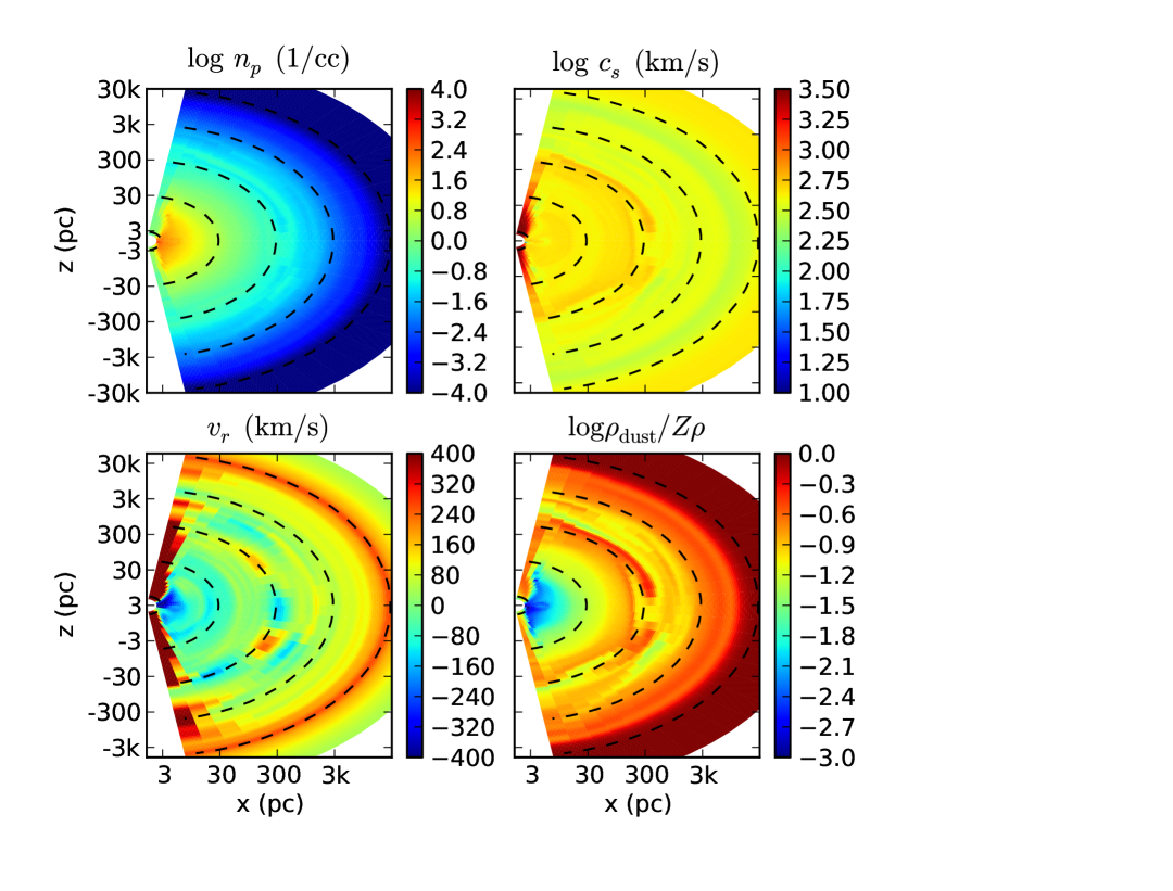
Figure 1: A snapshot of the A2 simulation during a quiescent phase. Upper left, log gas density in protons per cubic centimeter. Upper right, log sound speed. Lower left, radial velocity. Lower right, the log of the dust to gas ratio normalized to the value in the Milky Way. Gas that enters the ISM via the broad-line wind from the AGN is assumed to be dust rich. At small radii, densities and temperatures are large enough to efficiently destroy the dust grains, resulting in dust suppression by a factor of up to 1000.

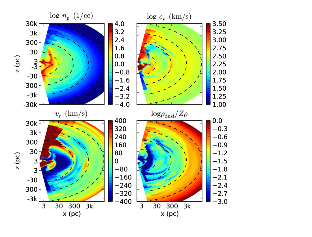
Figure 2: A snapshot of the A2 simulation during a black hole outburst. All gas near the center of the galaxy is depleted of dust by a factor of at least 30 and up to 1000.

Since stars are sources of UV and optical light that contribute to the solution to the radiative transfer equation discussed here, we briefly review our implementation of star formation and generation of star light. Gas that forms stars also contributes to the energy balance via supernovae, our implementation of which is discussed in detail in C07.

Gas is removed from the galaxy by star formation at the instantaneous rate given by the standard formula based on the Kennicutt (1998) law:

$$\dot{\rho}_{\rm gas}=-\frac{\eta_{\rm form}\rho}{t_{\rm form}}\,,\qquad\eta_{\rm form}=0.1\,,$$ (26)

$$t_{\rm form}=\max(t_{\rm cool},t_{\rm dyn})\,,$$ (27)

$$t_{\rm cool}=\frac{3k_{B}T}{2n\Lambda(T)}\,,\qquad t_{\rm dyn}=\min(t_{\rm jeans},t_{\rm rot})\,,$$ (28)

$$t_{\rm jeans}=\sqrt{\frac{3\pi}{32G\rho}}\,,\qquad t_{\rm rot}=\frac{2\pi r}{v_{c}(r)}\,,$$ (29)

where $n^{2}\Lambda(T)$ is the volumetric cooling function and $v_{c}(r)$ is the circular velocity at radius $r$ in the galaxy (Ciotti & Ostriker (2012)).

Mass that is transferred from gas to stars at radius $r$ is first transferred to a “forming” state by convolving the star formation rate with an exponential kernel with a time constant of $3\,\hbox{Myr}$, designed to account for the finite minimum star formation given by the Kelvin-Helmholtz timescale as well as the minimum stellar lifetime given by the combination of the Eddington luminosity and the nuclear energy available to a massive star:

$$\dot{\rho}_{\rm forming}(t)=-\frac{1}{t_{\rm KH}}\int_{0}^{t}\dot{\rho}_{\rm gas}(t^{\prime})e^{-\frac{t^{\prime}}{t_{\rm KH}}}\,dt^{\prime}\,.$$ (30)

These stars also contribute photons to the UV/optical luminosity of the galaxy via convolution with a similar exponential kernel:

$$\frac{dL_{B}}{dV}(t)=-\frac{1}{t_{B}}\int_{0}^{t}\epsilon_{B}c^{2}\dot{\rho}_{\rm gas}(t^{\prime})e^{-\frac{t^{\prime}}{t_{B}}}\,dt^{\prime}\,,$$ (31)

where $B$ refers to band and takes the values UV or optical. Values for $\epsilon_{B}$ and $t_{B}$ for each band are given in Table 2.

4.6 Radiative cooling and heating

Photons generated by collisional excitation of atomic lines or free-free radiation can only cool the ISM insofar as the photons can actually escape. If the galaxy becomes optically thick to IR radiation, then these photons can contribute significantly to the forces experienced by gas in the ISM as they diffuse out of the galaxy. Therefore we add the cooling radiation to the distributed UV (optical) source terms if the local gas temperature is above (below) $10^{5}\,\hbox{K}$. The radiative formulae are discussed in Ciotti & Ostriker (2012).

Table 2: Parameters governing stellar luminosities (see text for definitions)

Band	Fraction
$\epsilon_{\rm UV}$	$8.65\times 10^{-5}$
$\epsilon_{\rm Opt}$	$1.24\times 10^{-3}$
$t_{\rm UV}$	$2.57\,\hbox{Myr}$
$t_{\rm Opt}$	$154\,\hbox{Myr}$

4.7 Broad line wind

Our simulations also include a treatment of the broad-line wind generated near the SMBH. This is implemented as an inflow term on the edge of the computational grid (Novak et al., 2011; Ciotti & Ostriker, 2012). Although the present paper focuses on radiative AGN feedback, we summarize our implementation of mechanical feedback because it has a large effect on the regulation of black hole growth. See Novak et al. (2011) and Ostriker et al. (2010) for further discussion of mechanical feedback.

The BAL originating near the SMBH provides energy, momentum, and mass from a wind to the ISM according to the equations (Ostriker et al., 2010):

$$\dot{M}_{\rm BH}=\frac{\dot{M}_{\rm infall}}{1+\eta}\,,\qquad\eta=\frac{2\epsilon_{W}c^{2}}{v_{W}^{2}}\,,$$ (32)

$$\dot{E}_{W}=\epsilon_{W}\dot{M}_{\rm BH}c^{2}\,,\qquad\dot{P}_{W}=\frac{2\epsilon_{W}c^{2}\dot{M}_{\rm BH}}{v_{W}}\,,$$ (33)

and

$$\dot{M}_{W}=\frac{2\epsilon_{W}c^{2}\dot{M}_{\rm BH}}{v_{W}^{2}}\,,$$ (34)

where $v_{W}$ is the velocity of the BAL, taken here to be 10,000 km s^-1.

Independently of the mechanical feedback model, the radiative luminosity of the AGN is given by

$$L=\epsilon_{\rm EM}\dot{M}_{\rm BH}c^{2}\,,$$ (35)

where the electromagnetic efficiency is given by the advection dominated accretion flow inspired (Narayan & Yi, 1994) formula:

$$\epsilon_{\rm EM}=\frac{\epsilon_{0}A\dot{m}}{1+A\dot{m}}\,,$$ (36)

and $A=100$ and $\epsilon_{0}=0.1$. The dimensionless mass accretion rate is

$$\dot{m}=\frac{\dot{M}_{\rm BH}}{\dot{M}_{\rm Edd}}=\frac{\epsilon_{0}\dot{M}_{\rm BH}c^{2}}{L_{\rm Edd}}\,,$$ (37)

where $L_{\rm Edd}$ is the Eddington luminosity.

Although our other work has considered models where $\epsilon_{W}$ is a function of the accretion rate, in the present work we assume that $\epsilon_{W}$ is a constant with values given in Table 3. In previous papers these are called A models, and we maintain that nomenclature here. Our A0 model has the same value of $\epsilon_{W}$ as that adopted by Di Matteo et al. (2005), and our A2 model has a lower value, favored by recent observations (Moe et al., 2009; Arav et al., 2012).

Table 3: Values for the mechanical wind efficiency considered in this work.

Model	$\epsilon_{W}$
A0	$5\times 10^{-3}$
A2	$10^{-4}$

4.8 Galaxy model

The total gravitational potential of the model galaxy is assumed to be a singular isothermal sphere plus a point mass for the central BH. This is good agreement with observations of the total mass profile of early-type galaxies (Gavazzi et al., 2007; Gavazzi et al., 2008). For simplicity we maintain this model in to the smallest radii, although more complicated models may be more appropriate inside of a fraction of the half-light radius. The velocity dispersion parameter of the isothermal potential is 260 km s^-1. The gas is not self-gravitating. The stellar distribution is given by a Jaffe profile with a total mass of $3\times 10^{11}M_{\odot}$ and a projected half-mass radius of 6.9 kpc. The mass-to-light ratio is assumed to be spatially constant and is equal to 5.8 in solar units in the $B$ band at the present time. The structural and dynamical properties of these galaxy models are discussed in detail in Ciotti et al. (2009).

We note that although the galaxy model is spherically symmetric and the physics as implemented is either sperically symmetric or at least symmetric under inversions of the $z$ axis, numerical noise is quickly amplified chaotically in the simulations so that the physical state does not remain up/down symmetric for very long.

5 Results

All of the simulations presented here use the method described in Sections 3.2 through 3.3 to solve for the photon field, where the true boundary value problem is solved via the relaxation method.

Figures 1 and 2 show two snapshots from the “fiducial” A2 simulation with mechanical AGN feedback efficiency of $\epsilon_{W}=10^{-4}$ and all of the physics thus far described enabled. The dust to gas ratio is initialized to the Milky Way value throughout the galaxy. This simulation uses the “standard” recipe for dust grain creation where dust is created in supernova and dust grains do not not grow via collisions with gas-phase metal atoms in the ISM. However, all gas that enters the simulation grid does so with a Milky Way dust-to-gas ratio.

Figure 1 shows that near the center of the galaxy, dust is efficiently destroyed so that forces on gas due to absorption of photons by dust grains are not very effective at preventing gas from falling into the center of the galaxy. At large radius, the temperatures are sufficient for sputtering to be effective, but the gas densities are low enough that the grain destruction timescale is long.

In this picture, cold gas is generated by unstable cooling of the ISM. Cold gas loses pressure support and falls toward the center of the galaxy on a free-fall timescale. Cold gas is generated from hot gas, and the dust grains in the hot gas have been eroded by sputtering for for at least a cooling time. Therefore radiative forces on dust grains do not play a major role in the dynamics. Even if dust grains are replenished in the ISM without being processed through stars as suggested by Draine (2009), the grain growth timescale is at best comparable to the infall timescale. Given their initially depleted state, dust grains must have many growth timescales available in order to replenish the dust.

If radiative forces on dust are to play a role in black hole accretion, then the gas feeding the black hole must either never have been hot, or it must be cold for a long time before approaching the black hole. If the gas had been hot, it cannot return to the cold phase until a cooling time has passed, sufficient to significantly deplete the dust grains. Cold gas that is not rotationally supported falls to the center of the galaxy too quickly to build up significant dust. However, dust lanes are observed in a significant fraction of elliptical galaxies (Hawarden et al., 1981; van Dokkum & Franx, 1995). If the black hole is fed by gas processed through a rotationally supported galactic-scale disk, then dust grains would have a chance to build up while the gas spends a long time orbiting the black hole.

Figures 3 and 4 show black hole growth over 1 Gyr for the A0 and A2 simulations with mechanical feedback efficiencies of $5\times 10^{-3}$ and $10^{-4}$ respectively. In the former case, dust has little effect on the dynamics of the simulation because the mechanical feedback dominates over everything else. In the latter case, dust makes some difference, although it is not a dramatic effect. Furthermore, Figure 4 shows that occasionally the simulations with different assumptions about dust arrive at very similar black hole masses in spite of the black hole masses having been different at earlier times (e.g. at 200 Myr). This indicates that sometimes the dust affects when gas reaches the black hole, but not if gas reaches the black hole.

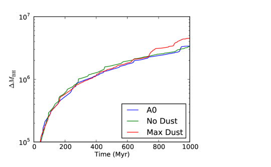
Figure 3: Black hole growth over 1 Gyr in the A0 simulation for different assumptions about the dust. The blue line shows the result of tracking dust density with a tracer field and accounting for dust creation and destruction. “No Dust” has all dust opacities set to zero. “Max Dust” assumes that all gas in the simulation has a Milky Way dust-to-gas ratio at all times. The high mechanical feedback efficiency in this simulation dominates over all other concerns and the presence or absence of dust does not make a significant difference.

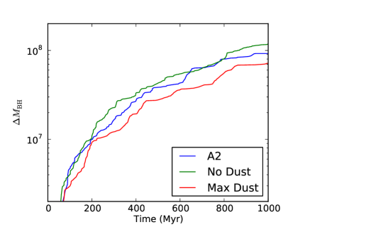
Figure 4: Black hole growth over 1 Gyr for the A2 simulation. The presence or absence of dust makes up to a factor of two difference in the black hole growth.

In our simulations, dust is not negligible in determining black hole growth, but neither is it dominant. Extreme assumptions about the dust-to-gas ratio ranging from no dust at all to constant Milky Way ratios makes at best a factor of two difference in the mass added to the black hole.

Figures 5 and 6 show the cumulative distribution of the ratio of the black hole accretion rate to the Eddington rate. The differences are not huge, but in the A2 case, dust opacity apparently does prevent the black hole from reaching the Eddington rate: the maximum is about 20% of the Eddington rate. The fraction of the time when the SMBH would be identified as a quasar ($L/L_{\rm Edd}>0.1$) is moderate.

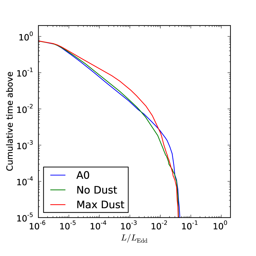
Figure 5: Cumulative time (in units of total elapsed time) where the ratio of the black hole accretion rate to the Eddington rate is above the given value for the A0 simulation with different assumptions about the dust to gas ratio. Dust does not make a big difference, although the “Max Dust” simulation spends somewhat more time with an Eddington ratio of $10^{-4}$ to $10^{-2}$ compared to the other simulations.

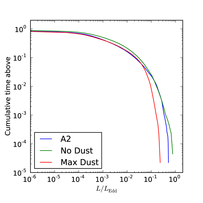
Figure 6: Cumulative time where the ratio of the black hole accretion rate to the Eddington rate is above the given value for the A2 simulation with different assumptions about the dust to gas ratio. Radiative forces on dust grains apparently prevent the black hole from reaching Eddington ratios greater than about 20%.

Figures 7 and 8 show the effect of various physical processes on the momentum balance of the ISM. These figures immediately show which physical processes dominate and which are negligible. It is important to note that these figures show the time averaged force per unit volume, so the dominant forces could change in the midst intense bursts of AGN accretion and star formation.

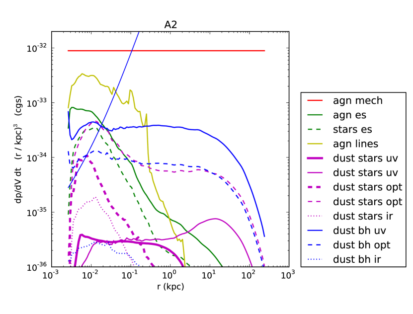
Figure 7: Time averaged radial momentum source and sink terms over 1 Gyr for the A2 simulation. Each line shows the time averaged force per unit volume imparted by each physical process as a function of radius. Curves have been multiplied by $(r/\mbox{kpc})^{3}$ to flatten them out. The thin rising blue line is gravity. Heavy lines are forces directed inward. Where a given physical process has both a heavy and light line, the force is sometimes directed inward and sometimes directed outward. The red line is for mechanical momentum. Mechanical momentum is injected at the first grid cell, so the quantity plotted is the force per unit volume if the momentum is deposited uniformly within a sphere of radius $r$. The green lines are for electron scattering of photons produced by the AGN or by stars, the yellow line is for photoionization by the AGN, the pink lines are for dust opacity for photons produced by the stars in different bands, and the blue lines are for dust opacity for photons produced by the AGN in different bands. The mechanical momentum accounts for the bulk of the momentum injected by feedback, and it will dominate at the radius at which the momentum is actually deposited into the ISM (typically $\simeq$1 kpc). Photoionization by the AGN (AGN lines) is important inside a few hundred parsecs, outside of which AGN UV photons acting on dust are important.

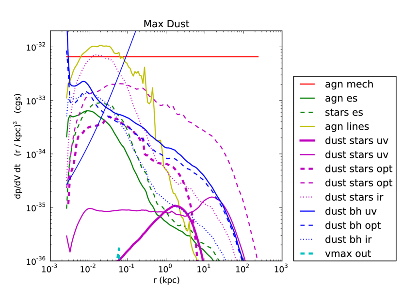
Figure 8: Radial momentum source and sink terms over 1 Gyr for the A2 simulation, assuming a Milky Way dust-to-gas ratio at all times. The lines and labels are the same as Figure 7 except for the cyan line, which shows the very small amount of momentum removed by limiting the gas velocity to $30,000\,\hbox{km}\,\hbox{s}^{-1}$. The most important momentum sources are the mechanical wind, photoionization by the AGN, and scattering of stellar IR photons by dust grains within about 1 kpc. Outside of 1 kpc, absorption of optical stellar photons by dust grains is the dominant source of momentum.

Most of the forces act on each grid cell separately, making it easy to tabulate how much momentum each separate process imparts to the ISM. Mechanical momentum is different: it is injected at the first grid cell and then the conservation equations of hydrodynamics transport that momentum outward until it mixes with the ISM and the wind stops. However, the wind termination is not abrupt and there are significant radial motions in the ISM even in the absence of a mechanical wind from the AGN, so determining the exact radius at which the mechanical wind deposits momentum is somewhat ambiguous. The quantity plotted as the red line in Figures 7 and 8 is the force per unit volume if the momentum is deposited uniformly within a sphere of radius $r$. Since the lines are also multiplied by $(r/\mbox{kpc})^{3}$, mechanical momentum shows up as a straight horizontal line. At very small radii, the “dentist drill” effect ensures that not much radial momentum is actually mixed into the ISM. The mechanical wind typically does not extend to the outer edge of the simulation grid, so likewise little momentum is actually deposited at large radius. Therefore the curve showing where the mechanical momentum is actually deposited would be low at small radii, low at large radii, nearly equal to the red line at intermediate radii (typically about 1 kpc) where the radial momentum is from the wind is actually mixed into the ISM.

For the A2 simulation with dust destruction allowed, the most important sources of radial momentum are the mechanical wind, photoionization by AGN photons, and absorption of UV AGN photons by dust grains. When dust destruction is not allowed and therefore the effects of dust are maximized, Figure 8 shows that the most important sources of momentum are the mechanical wind, photoionization by AGN photons, and dust scattering and absorption of optical and IR photons originating from stars. In the latter, maximal dust case, the effect of stellar photons on dust grains comes becomes more important than the effect of AGN photons on dust grains for three reasons: 1) the black hole mass is about a factor of two smaller, so the black hole produces fewer photons; 2) about 20% more stars are formed, so stellar luminosity is increased; 3) the stars that form are much more centrally concentrated (about a factor of two more stars inside of 1 kpc), so the outgoing stellar photons see a larger optical depth to dust absorption because the density of the ISM falls steeply with radius

It is somewhat surprising that dust seems to have such a small effect on the black hole growth in the simulation, given that the opacity in the UV due to dust is 3500 times the electron scattering opacity. Therefore, at least in the “Max Dust” case where a Milky Way dust to gas ratio is assumed for all gas, one might expect that the effective limit to the black hole accretion rate is $\sim$1/3500 times the Eddington rate. However, the crucial crucial difference is that radiative transfer is governed by the absorption opacity in the UV while electron scattering and the transfer of thermal IR photons is a scattering problem. Once the UV has been absorbed, the radiative transfer in the IR is, again, essentially a scattering problem with $\kappa_{\rm IR}=5.71\kappa_{\rm ES}$; however, dust to gas ratios in elliptical galaxies are depleted as compared to the Milky Way by more than the modest factor of five required for electron scattering to dominate over dust scattering.

As noted by Thompson et al. (2005) and Murray et al. (2005) in the context of this problem, the force exerted on a shell of gas by photons where scattering dominates is:

$$f=\frac{L\tau}{c}\,,$$ (38)

where $L$ and $\tau$ are the luminosity of the source and optical depth of the shell, both defined in the given frequency band. The energy in photons cannot be destroyed, so if the shell is optically thick, then photons build up until the gradient of the photon number density is sufficient for diffusion to carry the input luminosity. This is why the Eddington luminosity effectively limits the black hole accretion rate even for Compton-thick sources, with the caveat that some energy is transferred to thermal energy in the gas by inelastic scattering of photons with energies of order 1 MeV. The Eddington limit remains the relevant limit until the optical depth to electron scattering becomes so large that the photon diffusion time is larger than the gas inflow time, in which case the photons are advected into the black hole along with the gas in a radiatively inefficient accretion flow.

However, the situation is quite different when the total opacity is dominated by absorption. For UV photons emitted by the black hole, the force exerted on a shell of gas is:

$$f=\frac{L\min(\tau,1)}{c}\,.$$ (39)

The incident UV photons deliver their momentum to the shell, after which they are converted to thermal IR photons where the opacity is much smaller. The thermal IR photons then simply leave the galaxy without further scattering until the galaxy becomes optically thick in the IR. The crucial point is that UV photons cannot build up and then diffuse out of the galaxy, as is the case when considering the electron scattering opacity and the dust opacity in the IR. The maximum force that can be exerted on a shell of gas is $f_{\rm UV}L/c$ where $f_{\rm UV}$ is the fraction of the black hole bolometric luminosity that is emitted in the UV.

If the infalling clouds of gas are optically thin in the UV, then the force on a gas cloud is

$$f=\frac{L(f_{\rm UV}\tau_{\rm UV}+\tau_{\rm ES})}{c}\simeq\frac{L\tau_{\rm ES}}{c}\frac{f_{\rm UV}\kappa_{\rm UV}}{\kappa_{\rm ES}}\,,$$ (40)

where $L$ is the bolometric luminosity and $f_{\rm UV}$ is the fraction of the bolometric luminosity emerging in the UV. The cloud will feel a force much larger than if the dust opacity were not considered. However, if the cloud is optically thick in the UV (but not in the IR) then the force is

$$f=\frac{L(f_{\rm UV}+\tau_{\rm ES})}{c}\,.$$ (41)

In this case, the force is nearly independent of the mass of the cloud; adding mass to an already optically thick cloud increases the gravitational force but not the opposing radiative force. This fact makes it difficult for the dust opacity in the UV to have a dramatic effect on the gas falling toward the black hole.

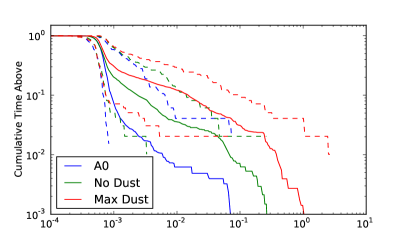
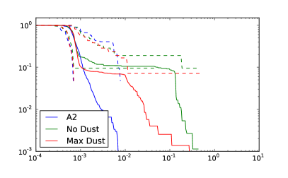
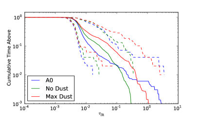
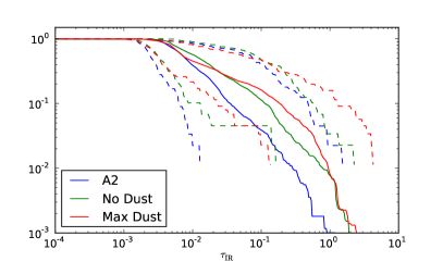
Figure 9: In the upper two panels, the cumulative distribution of optical depths due to dust in the IR using the tracer field that tracks dust creation and destruction in the simulation to calculate the dust opacity. The lower two panels show the same quantity assuming a constant dust-to-gas ratio (corresponding to values appropriate for the Milky Way) so that the optical depth scales directly with the column density of the gas. For solid lines, each line of sight in each snapshot contributes separately to the distribution. Dashed lines show the distributions where only the line of sight with the highest or lowest optical depth from each snapshot contribute. The simulations only rarely become optically thick in the IR, and when this happens, the optical depth is only a few times unity. Furthermore, the distribution of minimum optical depths shows that there are always optically thin lines of sight available that allow photons to exit the galaxy without scattering multiple times. For the simulations labeled “No Dust,” the simulation neglects any radiative forces associated with dust, but it nevertheless tracks the dust tracer field, allowing those simulations to be included in these plots.

Figure 9 shows the distribution of optical depths for the A0 and A2 simulations and variants. The typical optical depths are far below unity, although a small fraction of the time the simulations become optically thick, at least along some lines of sight. However, the distribution of minimum optical depths for each simulation snapshot show that there are almost always optically thin lines of sight available that will allow IR photons to escape without experiencing multiple scatterings that are necessary for eq. (38) to be relevant.

In spite of dust having at best a minor effect on the dynamics of the ISM, it has a dramatic effect on the radiation emerging from the galaxy. With no dust grain destruction, the optical depth in the UV from the center of the galaxy is typically of order unity. This means that the typical UV photon from the black hole is absorbed on its way out of the galaxy. Therefore observations of the AGN will be dramatically different for different assumptions about the creation and destruction of dust, even if the dust does not dramatically affect the dynamics of the galaxy.

Absorbed UV/optical photons from the AGN are converted to IR photons, but the galaxy is typically quite optically thin in the IR, so these photons escape without much fanfare. If the ISM were optically thick to IR photons, then they could have a dramatic effect as they scatter out of the galaxy, as pointed out by Murray et al. (2005) and Thompson et al. (2005), but we do not find the conditions necessary for this effect to prevail in our simulations. We find that in our detailed treatment of the radiative transfer, the factor $\tau$ in eq. (38) never exceeds unity by a significant amount.

Most stellar UV/optical photons are not absorbed because the star light is emitted at larger radius and need not traverse the densest part of the ISM. The typical stellar UV photon is produced at roughly the half-light radius of the galaxy, from which point the typical optical depth is far less than unity. Therefore the stellar emission is largely unaffected by dust in the galaxy. Dramatically different assumptions about the dust to gas ratio have a minor effect on both the dynamics due to and the observations of stellar photons.

A subtlety arises when considering the distributed radiation source (the stars) in the case where the ISM is optically thick to absorption and the gas density is falling steeply (faster than $r^{-1}$). In this case it is possible for the luminosity at a given radius to be negative, i.e. the net flux points inwards. If there were no absorption, then every ingoing photon would eventually become an outgoing photon, either by traveling unimpeded and emerging at a different point on the same sphere of radius $r$, or else by scattering until it diffused to radius $r$. This must be the case or else photons would build up at radii smaller than $r$.

However, when absorption is important, UV photons may propagate inward, undergo absorption, and re-emerge as IR photons. If the density profile is steep enough, this situation robustly leads to negative UV luminosities for radii smaller than the radius from which the typical UV photon is emitted. That is to say that the stars at larger radius exert a force acting to compress gas near the center of the galaxy. The force is not balanced by outgoing IR photons (which must after all carry the energy of UV photons absorbed at small radius) because the opacity is smaller in the IR. The momentum carried by the IR photons is deposited at larger radius.

We find that this is often the case in our simulations: the gas density profile is generally steep enough to permit negative luminosities to develop within a few kiloparsecs of the center of the galaxy. This effect can be seen in Figures 7 and 8.

There are situations in which dust plays a major role, such as galaxies undergoing starbursts or merger-induced quasar activity with copious quantities of cold gas (Murray et al., 2005; Thompson et al., 2005; Debuhr et al., 2010; Debuhr et al., 2011). We have performed one simulation designed to be similar to an ultra-luminous infra-red galaxy having a star formation rate of several hundred solar masses per year. The simulation uses the A2 feedback parameters but starts with $3\times 10^{10}M_{\odot}$ of gas, corresponding to a gas fraction of 10%, as could be induced by a major merger or an inflow of cold gas. The star formation rate reaches peaks of 200 solar masses per year, approaching the ULIRG conditions.

Figure 10 shows the distribution of Eddington ratios for different assumptions about the dust to gas ratio in this simulation. The simulation that includes dust creation and destruction is quite similar to the maximum dust case because the short dust creation time ensures that most of the gas has a dust to gas ratio near that of the Milky Way, as is observed in the ULIRG case. Assuming that there is no dust in the simulation yields a dramatically different distribution of Eddington ratios, reaching much larger values. The time averaged black hole accretion rates are 0.045 $M_{\odot}\,\hbox{yr}^{-1}$ for the case with maximal dust, 0.061 $M_{\odot}\,\hbox{yr}^{-1}$ for the case with dust creation and destruction, and 0.32 $M_{\odot}\,\hbox{yr}^{-1}$ for the case with no dust. Thus the presence of dust may suppress black hole growth by a factor of five to seven depending on the assumptions surrounding dust creation and destruction.

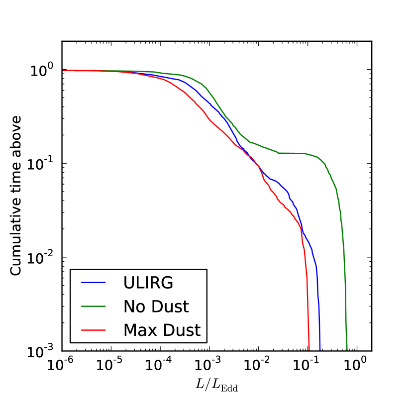
Figure 10: Cumulative time where the ratio of the black hole accretion rate to the Eddington rate is above the given value for a simulation designed to resemble a ULIRG with different assumptions about the dust to gas ratio. For large enough gas column densities, radiative effects due to dust opacity have a large effect, and a careful treatment of dust production and destruction produces results similar to the “Max Dust” case, with “ULIRG” SMBH luminosity in the quasar range for several percent of the time.

The reason for this is that the conditions now resemble those envisioned by Thompson et al. (2005) and Murray et al. (2005): the gas surface density is high enough that the galaxy is optically thick in the infrared. The infrared photons build up in the galaxy until the gradient of the photon number density is sufficient to carry the black hole luminosity by photon diffusion. In this case, the relevant opacity to limit accretion is not the electron scattering opacity but the dust opacity in the infrared. Dust then has a dramatic effect on the gas dynamics and on the growth of the black hole.

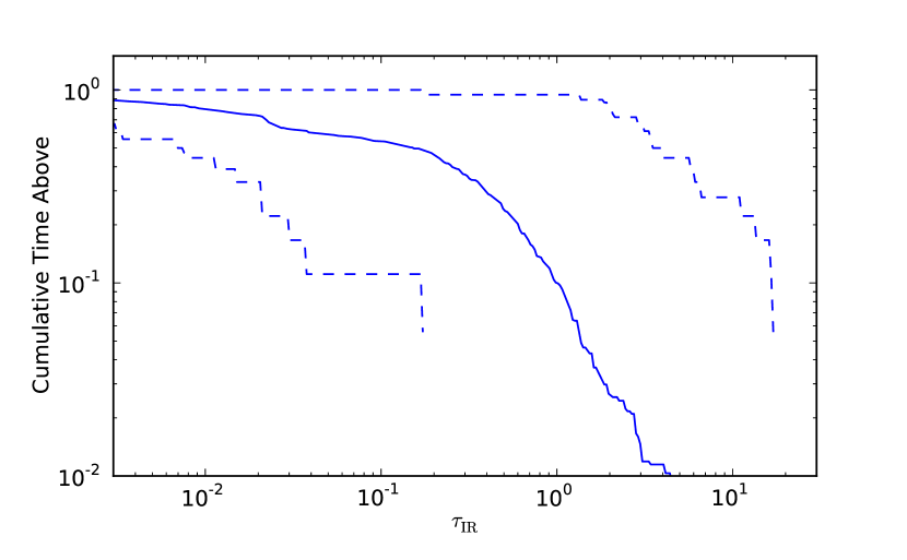
Figure 11: Cumulative distribution of optical depths due to dust in the IR for the simulation designed to resemble a ULIRG. The “Max Dust” case is shown, but high gas densities resulted in sufficiently fast dust creation that the other cases do not differ significantly. Typical optical depths along a typical line of sight are of order unity. There are almost always optically thick lines of sight where the optical depth is larger than ten a significant fraction of the time. However, even in this case there are always optically thin lines of sight that would allow photons to easily escape from the galaxy.

Figure 11 shows the cumulative distribution of optical depths due to dust in the IR for the ULIRG-like simulation. Along some lines of sight, the situation resembles that envisioned by Thompson et al. (2005) and Murray et al. (2005) a significant but sub-dominant fraction of the time—optical depths are a few times unity and can exceed ten. However, the distribution of minimum optical depths for each simulation snapshot shows that IR photons would always be able to escape via optically thin “windows”. In order for equation 38 to pertain, the IR photons must be effectively trapped in the galaxy so that the only way for them to exit the galaxy is via diffusion. If there are optically thin lines of sight, this will not occur.

6 Discussion and Conclusions

We have outlined a method for computing the forces on interstellar gas due to absorption of photons by dust grains. The radiative transfer equation is recast into a set of differential equations by taking moments in the photon propagation direction. The set of differential equations comprises a boundary value problem, the solution of which gives the photon field which can be used to compute forces on the ISM. We identified a numerical method that reliably gives the solution to the set of differential equations even for very large optical depths.

The method gives the correct asymptotic behavior in all of the relevant limits (dominated by the central point source; dominated by the distributed isotropic source; optically thin; optically thick to UV/optical; optically thick to IR; photon field nearly isotropic; photon field highly directed) and reasonably interpolates between the limits when necessary. The method is explicitly energy conserving so that UV/optical photons that are absorbed are not lost, but are rather redistributed to the IR where they may scatter out of the galaxy. It does not require spherical symmetry, but it only handles the radial component of radiative forces.

We have also described a physically motivated simplification of the above method based on splitting the photon field into ingoing and outgoing streams. This method is much simpler to implement and shares many of the desirable characteristics of the more complicated method.

We have implemented both of these numerical methods in a hydrodynamic code with source terms for energy, momentum, and mass appropriate to study black hole fueling and star formation in early type galaxies. Both radiative and mechanical feedback are included for both the AGN and the stars. We allow for dust destruction by sputtering and dust creation by supernovae, planetary winds, and optionally gas-phase grain growth.

In the case of secular fueling of a normal SMBH in an elliptical galaxy, the dynamics of the simulations are not greatly affected by the presence or absence of dust. At high AGN mechanical feedback efficiencies, dust has very little effect because mechanical feedback dominates. At lower mechanical feedback efficiencies, dust has some effect but large changes in our assumption about the dust-to-gas ratio lead to measurable but relatively modest changes in the black hole growth, star formation, and galactic winds. This is true even for extreme assumptions about dust, ranging from no dust at all to assuming dust-to-gas rations appropriate to the Milky Way pertain at all times. Allowing for the possibility of dust destruction by sputtering in hot gas makes the simulations behave similarly to the “No Dust” case.

If the galaxy is optically thick to IR photons, repeated scattering of these photons can have a dramatic effect on the momentum balance of the ISM. We have verified this by simulating a galaxy with a very large mass in the ISM, as might follow a major merger with a gas rich galaxy, in which case the presence or absence of dust makes a large difference, as expected.

However, we do not find that this situation is typically realized in our simulations. The opacity of dust in the IR is about five times the electron scattering opacity, so a system must be Compton thick before this scattering starts to have a large effect. Our simulated galaxies are occasionally Compton thick, but no more, and they typically have much lower column densities. Even with no dust destruction, we find that the optical depth in the IR is at most a few times unity, and it reaches that value only for a small fraction of the total simulation time. We find that it is very rare for the optical depth in the IR to significantly exceed unity, as is assumed by Debuhr et al. (2010); Debuhr et al. (2011). When dust destruction is allowed, the optical depths in the IR is typically smaller by several orders of magnitude.

Appendix A Third order radiation transport

The quality of a solution to the radiation transport equation obtained by taking moments depends on the accuracy of the physical assumptions implicit in the chosen analytic form for the specific intensity. If those assumptions are not satisfied, taking the expansion to higher order is unlikely to provide benefits commensurate with the costs in terms of complexity and computational resources. We believe that the assumptions embodied by eqs. (3) and (12) are quite reasonable for the problem at hand. Nevertheless, it is possible to avoid using eq. (12) by taking one additional moment of the specific intensity and radiation transport equation. We provide the equations here for reference but do not pursue the method further in the present paper.

Define the third moment of the specific intensity to be:

$$Q\equiv\int_{0}^{2\pi}d\phi\int_{-1}^{1}\mu^{3}I(\mu,\phi)\,d\mu\,.$$ (42)

Given eq. (3) we find

$$Q=\frac{4\pi B}{5}+\pi D\,.$$ (43)

We have three constants in the assumed form of the mean intensity and four moments of the mean intensity, so we can solve for the closure relation:

$$Q=\frac{4\pi J+3F+3cP}{5}\,.$$ (44)

To obtain the differential equations, we take the equations for the zeroth and first moment derived above, supplement them with the second moment of the radiation transport equation, and then insert the closure relation to obtain the following set of three equations:

$$\frac{dJ}{dr}+\frac{7J}{r}-\frac{F}{\pi r}+\frac{3cP}{4\pi r}=\rho\left(3\kappa_{a}+\frac{5\kappa_{s}}{3}\right)J-\frac{\dot{E}}{3\pi}$$

$$+\frac{\rho(\kappa_{a}+\kappa_{s})(3F-5cP)}{4\pi}\,,$$ (45)

$$\frac{dL}{dr}=4\pi r^{2}(\dot{E}-4\pi\rho\kappa_{a}J)\,,$$ (46)

and

$$c\frac{dP}{dr}-\frac{4\pi J}{r}+\frac{3cP}{r}=-\rho(\kappa_{a}+\kappa_{s})F\,.$$ (47)

Adopting the use of these equations and closure relation is perhaps formally more appealing than the method outlined in Section 3. However, the cost is one additional equation to integrate and perhaps less obvious physical content to the closure relation and the equations themselves. We have included the present equations for reference, but do not use this method of obtaining solutions to the radiation transport problem in the present work.

Appendix B Simplified radiation transport

In Section 3 we have described a complete algorithm to solve for the photon field and, subsequently, the radiative forces on interstellar gas. The algorithm is exact in the sense that if the physical approximations used in its derivation are correct, the method will compute the correct photon field and radiative forces.

However, solving for the radiation field dominates the computational resources required for the calculation primarily because the system differential describes a boundary value problem rather than an initial value problem and hence finding the solution requires iteration. We would like a another solution method that is computationally efficient while respecting the essential physics of the previously defined algorithm.

Consider the problem where the only source of radiation is the black hole and the scattering opacity is zero. The UV/optical photons are always radially outgoing at all times. Some UV/optical photons are converted to IR photons which diffuse out of the galaxy, but the UV/optical radiation field never becomes isotropic. In this case the flux is simply related to the mean intensity ($F=4\pi J$) and we can eliminate eq. (11) to obtain the single equation for the UV and optical components

$$\frac{dL}{dr}=-\rho\kappa_{a}L\,.$$ (48)

The boundary condition is $L(r_{\rm min})=L_{\rm BH}$. This is now an initial value problem rather than a boundary value problem, and can be trivially solved by integrating from the inner edge of the simulation grid.

This change greatly simplifies the solution procedure. It would be very useful to obtain a simple approximate treatment of this problem that as an initial value problem rather than a boundary value problem. We seek such an algorithm presently.

B.1 Differential equations

Conceptually, there are two streams of radiation: an ingoing stream and an outgoing stream. If the optical depth is low, then the photons in the ingoing stream are likely to successfully traverse the inner parts of the galaxy and emerge as outgoing photons. In this case, all of the radiation emitted by stars should be considered to be added to the outgoing stream. Doing so gives the correct forces on the material inside and outside the emitting sphere due to the well-known result that for a inverse square force law, there is no net force on a test particle inside a spherical shell of material; and a test particle outside the spherical shell feels a force equal to that of a point source of equivalent mass, charge, or luminosity, no matter whether the force is gravitational, electrostatic, or due to momentum transfer by photons.

If the optical depth is large, then the ingoing photons are likely to be absorbed in the inner part of the galaxy. Then only half of the emitted photons should be added to the outgoing stream. The other half should be added to the ingoing stream, where they will in due course be absorbed.

This leads to the following two equations:

$$\frac{dL_{\rm out}}{dr}=4\pi r^{2}\Psi\dot{E}-\rho\kappa_{a}L_{\rm out}\,,$$ (49)

and

$$\frac{dL_{\rm in}}{dr}=4\pi r^{2}(1-\Psi)\dot{E}-\rho\kappa_{a}L_{\rm in}\,,$$ (50)

where $\Psi$ is the fraction of photons emitted at a given radius that are likely to become outgoing photons, either because they were emitted in the outward direction, or because they were emitted inward but are likely to successfully traverse that region without being absorbed.

B.2 Solving the differential equations

The boundary conditions are $L_{\rm out}(r_{\rm min})=0$ and $L_{\rm in}(r_{\rm max})=0$, so that eq. (49) is solved by integrating outward and eq. (50) is solved by integrating inward.

Summing eqs. (49) and (50) simply gives eq. (10), as expected. The advantage of splitting the radiation into an ingoing stream and an outgoing stream is that it transforms a boundary value problem into an initial value problem, leading to a great reduction of the effort required to find a numerical solution. The quality of the solution will depend on the accuracy of the function $\Psi$ is estimating the contribution that the stars at a given radius make to the ingoing and outgoing streams of radiation. This can of course be checked by comparing to the solution obtained by solving the full boundary value problem.

We have found that this scheme gives reasonable results at a fraction of the algorithmic complexity and computational cost of obtaining the exact solution. Figure 12 shows the results of solving the radiation transfer equation by the simplified two-stream method and the full solution obtained by solving the boundary value problem for one line of sight in one simulation snapshot. The total optical depth along the line of sight is 13.5. The solution given by the simplified scheme is not perfect, but it is remarkably good given the large optical depth and the reduced algorithmic and computational cost.

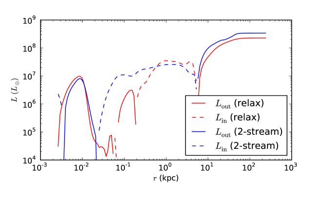
Figure 12: The luminosity as a function of radius for the full relaxation based algorithm (Section 3.2) and the simpler two-stream based algorithm (Appendix B). Dashed lines indicate inward-directed luminosities. The solution given by the two-stream approximation described in Appendix B has about 50% more flux at infinity than the “true” solution, and it misses the true solution around 100 pc. However, the solution is quite good given the gains in algorithmic simplicity and reduced computational costs. The function $\Psi$ associated with $\zeta=2$ was used for this figure, where $\zeta$ is the index of the assumed power law dependence of photon mean free path on radius used in defining $\Psi$ (see Appendix B.3 for details).

B.3 Concerning $\Psi$

If $p_{\rm abs}$ is the probability that a given ingoing photon is absorbed before again reaching the radius at which it was emitted (and hence becoming an outgoing photon) and $p_{\rm trans}=1-p_{\rm abs}$ is the probability that a given ingoing photon is transmitted so that it again arrives at the radius at which it was emitted and becomes an outgoing photon, then:

$$\Psi\equiv 1-\frac{p_{\rm abs}}{2}=\frac{1+p_{\rm trans}}{2}$$ (51)

The probabilities for absorption and transmission appear in eqs. (49) and (50) only through the quantities $\Psi$ and $1-\Psi$. Note that of the four ways of writing $\Psi$ and $1-\Psi$ in terms of transmission and absorption probabilities, $p_{\rm abs}$ and $p_{\rm trans}$ are added to an order-unity constant in all cases except one: $1-\Psi=p_{\rm abs}/2$. An argument could be made that one should take special care to obtain the correct asymptotic behavior for $p_{\rm abs}$ when $p_{\rm abs}\ll 1$ in order to avoid large fractional errors in the ingoing radiation stream. However, this is the optically thin limit, exactly where the ingoing radiation stream is expected to be of limited importance. Therefore any expression for $\Psi$ with the correct asymptotic limits and a transition between the two limits when the system goes from optically thin to optically thick conditions should introduce only limited fractional errors into eqs. (49) and (50).

The simplest estimate of the fraction of photons emitted at a given radius that are likely to be absorbed at smaller radii comes from finding the apparent size of the sphere where $\tau=1$ as seen from the radius $r$, where the photons are emitted.

$$\Psi=1-\frac{1}{2}\left[\frac{1}{1+e^{-\tau}}\right]\left[\frac{r_{1}^{2}}{\max(r_{1}^{2},r^{2})}\right]\,,$$ (52)

where $\tau$ is the optical depth from $r$ to infinity, $\tau=\int_{r}^{\infty}\rho\kappa\,dr$, and $r_{1}$ is the radius where the optical depth is unity: $1=\int_{r1}^{\infty}\rho\kappa\,dr$. Here the factor $1/(1+e^{-\tau})$ interpolates between the correct asymptotic expressions for the case where $\tau\ll 1\,,\,r_{1}\ll r$, in which $\Psi\simeq 1-0.5r_{1}^{2}/r^{2}$ and the case where $\tau\gg 1\,,\,r_{1}\gg r$ in which $\Psi\simeq 1/2$.

More rigorous formulae can be derived assuming spherical symmetry and a power-law dependence of the mean free path for absorption on the radius. Given the geometry shown in Figure 13, the optical depth as a function of the angle $\alpha$ between the direction of the ray and the line connecting the emission point to the center of the coordinate system is

$$\tau(\alpha)=\int_{0}^{\pi-2\alpha}\frac{r\sin\alpha\,d\beta}{\sin^{2}(\alpha+\beta)\,l\left(\frac{r\sin\alpha}{\sin(\alpha+\beta)}\right)}\,,$$ (53)

where $r$ is the radius of emission, $l(s)\equiv 1/\rho(r)\kappa(r)$ is the mean free path to absorption and $\alpha$, $\beta$, and $s$ are defined by Figure 13. The formula gives the optical depth for a photon to traverse the chord of the circle in Figure 13.

Figure 13: Geometry for calculation of optical depth in Section B.3

If the mean free path as a function of radius can be approximated by a power law

$$l(s)\approx l_{0}\left(\frac{s}{r}\right)^{\zeta}\,,\qquad\zeta>0$$ (54)

where $l_{0}$ is the local mean free path at the radius $r$ at which the photons are emitted, then eq. (53) can be written in terms of hypergeometric functions. However, assuming that $\zeta$ is an integer gives the simple formulae involving elementary functions given in Table 4

Table 4: Optical depth as a function of photon emission direction in the case of a power-law mean free path, where $\zeta$ is the power-law index.

$\zeta$	$\tau(\alpha)$
0	$(2r/l_{0})\cos\alpha$
1	$(2r/l_{0})\log\cot(\alpha/2)$
2	$(r/l_{0})(\pi-2\alpha)/\sin\alpha$
3	$(2r/l_{0})\cos\alpha/\sin^{2}\alpha$
4	$(r/2l_{0})(\pi-2\alpha+\sin 2\alpha)/\sin^{3}\alpha$

The transmission probability $p_{\rm trans}$ is then

$$p_{\rm trans}=\int_{0}^{\pi/2}\sin\alpha\,e^{-\tau(\alpha)}\,d\alpha\,,$$ (55)

so that $\Psi$ can be recovered from eq. (51).

The integral in eq. (55) unfortunately cannot be expressed in terms of elementary functions. However, for a given dependence of mean free path on radius, it is a function only of the radius in units of the local mean free path $r/l_{0}$. For integral values of $\zeta$ the integrand consists of elementary functions, so it can be tabulated at the beginning of a calculation and used throughout with little computational cost. For values of $\zeta$ from 0 to 4 (corresponding to cases from $\rho=$ constant to $\rho\propto r^{-4}$ if the opacity is constant), the values of $p_{\rm trans}$ and $p_{\rm abs}$ do not depend sensitively on $\zeta$.

Figure 14 shows $p_{\rm abs}$ and $p_{\rm trans}$ as the as a function of optical depth for different values of $\zeta$. The precise value of $\zeta$ makes a moderate difference when the mean free path is roughly equal to the radius of the sphere. In the optically thick limit, the asymptotic form of $p_{\rm trans}$ is independent of $\zeta$ and is given by

$$p_{\rm trans}\approx 0.005\left(\frac{l_{0}}{100\,r}\right)\,,\quad\mbox{for}\quad l_{0}\ll r\,.$$ (56)

For the optically thin case, the asymptotic value of $p_{\rm abs}$ depends on $\zeta$. For values of $\zeta$ from 0 to 4, the asymptotic form can be approximated as:

$$p_{\rm abs}\approx\frac{1}{100}\left[1+6\left(\frac{\zeta}{4}\right)^{2}\right]\left(\frac{\zeta}{4}\right)^{-1+0.4(\zeta/4)^{3}}\,,\quad\mbox{for}\quad l_{0}\gg r\,.$$ (57)

Figure 14: Probability of transmission and absorption for spherically symmetric systems with power-law mean free paths of index $\zeta$. Solid lines give $p_{\rm abs}$, dashed lines give $p_{\rm trans}$.

Following the dictum discussed above that errors in $p_{\rm trans}$ are tolerable because $p_{\rm trans}$ is always added to an order unity constant, while the same is not true for $p_{\rm abs}$ for the ingoing radiation stream when $p_{\rm abs}$ is small, then one may take the approximation:

$$p_{\rm abs}=\frac{\tilde{p}_{\rm abs}}{1+\tilde{p}_{\rm abs}}\,,$$ (58)

with $\tilde{p}_{\rm abs}$ given by eq. (57) over the whole range of optical depths. The value of $\Psi$ may then be recovered using equation 51.

References

- Arav et al. (2012) Arav N., Dunn J. P., Korista K., Edmonds D., González-Serrano J. I., Benn C., Jiménez-Luján F., 2012, BAL Outflow Contribution to AGN Feedback: WHT Observations of QSO 1044+3656, ApJ, submitted
- Barai et al. (2011) Barai P., Proga D., Nagamine K., 2011, MNRAS, 418, 591
- Binney & Tabor (1995) Binney J., Tabor G., 1995, MNRAS, 276, 663
- Booth & Schaye (2009) Booth C. M., Schaye J., 2009, MNRAS, 398, 53
- Brandt et al. (2011) Brandt T. D., Burrows A., Ott C. D., Livne E., 2011, ApJ, 728, 8
- Chandrasekhar (1960) Chandrasekhar S., 1960, Radiative transfer. New York: Dover, 1960
- Choi et al. (2012) Choi E., Ostriker J., Naab T., Johansson P., 2012, Radiative and Momentum Based Mechanical AGN Feedback in a 3-Dimensional Galaxy Evolution Code, In prep.
- Ciotti et al. (2009) Ciotti L., Morganti L., de Zeeuw P. T., 2009, MNRAS, 393, 491
- Ciotti & Ostriker (1997) Ciotti L., Ostriker J. P., 1997, ApJ, 487, L105
- Ciotti & Ostriker (2001) Ciotti L., Ostriker J. P., 2001, ApJ, 551, 131
- Ciotti & Ostriker (2007) Ciotti L., Ostriker J. P., 2007, ApJ, 665, 1038
- Ciotti & Ostriker (2012) Ciotti L., Ostriker J. P., 2012, in D.-W. Kim & S. Pellegrini ed., Astrophysics and Space Science Library Vol. 378 of Astrophysics and Space Science Library, AGN Feedback in Elliptical Galaxies: Numerical Simulations. p. 83
- Ciotti et al. (2009) Ciotti L., Ostriker J. P., Proga D., 2009, ApJ, 699, 89
- Ciotti et al. (2010) Ciotti L., Ostriker J. P., Proga D., 2010, ApJ, 717, 708
- Cisternas et al. (2011) Cisternas M., et al., 2011, ApJ, 726, 57
- Croton et al. (2006) Croton D. J., Springel V., White S. D. M., De Lucia G., Frenk C. S., Gao L., Jenkins A., Kauffmann G., Navarro J. F., Yoshida N., 2006, MNRAS, 365, 11
- Daddi et al. (2007) Daddi E., Alexander D. M., Dickinson M., Gilli R., Renzini A., Elbaz D., Cimatti A., Chary R., Frayer D., Bauer F. E., Brandt W. N., Giavalisco M., Grogin N. A., Huynh M., Kurk J., Mignoli M., Morrison G., Pope A., Ravindranath S., 2007, ApJ, 670, 173
- Davis et al. (2007) Davis M., et al., 2007, ApJ, 660, L1
- Debuhr et al. (2010) Debuhr J., Quataert E., Ma C., Hopkins P., 2010, MNRAS, 406, L55
- Debuhr et al. (2011) Debuhr J., Quataert E., Ma C.-P., 2011, MNRAS, 412, 1341
- Debuhr et al. (2012) Debuhr J., Quataert E., Ma C.-P., 2012, MNRAS, 420, 2221
- Di Matteo et al. (2005) Di Matteo T., Springel V., Hernquist L., 2005, Nature, 433, 604