Global Superfluid Phase Diagram of Three Component
Fermions with Magnetic Ordering

Abstract

We investigate a three component fermion mixture in the presence of weak attractive interactions. We use a combination of the equation of motion and the Gaussian variational mean-field approaches, which both allow for simultaneous superfluid and magnetic ordering in an unbiased way, and capture the interplay between the two order parameters. This interplay significantly modifies the phase diagram, especially the superfluid-normal phase boundaries. In the close vicinity of the critical temperature and for small chemical potential imbalances, strong particle-hole symmetry breaking leads to a phase diagram similar to the one predicted by Cherng et al. [Phys. Rev. Lett. 99, 130406 (2007)], however, the overall phase diagram is markedly different: new chemical potential-driven first and second order transitions and triple points emerge as well as more exotic second order multicritical points, and bicritical lines with $O(2,2)$ symmetry. We identify the terms which are necessary to capture this complex phase diagram in a Ginzburg-Landau approach, and determine the corresponding coefficients.

I Introduction

Experiments with ultracold atoms opened a fascinating way to study strong correlations and the emergence of exotic phases in a controlled way.Zwerger Paradigmatic solid state physics models such as the fermionic and bosonic Hubbard models have been realized, Mott insulating and magnetic phasesBoseMott ; FermiMott as well as various kinds of fermionicSfExperiment1 ; SfExperiment2 ; FFLOExp1 ; FFLOExp2 ; DensityJumpExp ; Vortices and bosonicBoseMott ; BosonicSuperfluids superfluid phases have been observed. Topological excitations, e.g. vorticesFFLOExp2 ; Vortices , solitonsSolitons , 2D and 3D skyrmionic excitationsSkyrmions , and knot configurationsKnots have been subjects to intensive research. Introduction of artificial gauge fields has also been considered both theoretically and experimentallyGaugeFields , indicating that the realization of the quantum-Hall effect and related phenomena with cold atoms are within reach.

Cold atomic systems provide, however, not only a way to study models emerging in solid state physics, but they were also proposed to be used to mimic phenomena appearing in high energy and particle physics. In particular, attractive three component mixtures have been proposed to simulate quark color superfluidityHonerkampHofstetter and ”baryon” formation,Rapp two fundamental concepts of quantum chromodynamics (QCD). An experimental realization of these mixtures is very difficult, but not hopeless: although three component systems are plagued by 3-particle losses,OHara ; Zoller ; GrimmEfimov nevertheless, Fermi degeneracy has been reached in ⁶Li systems,ThreeCompDegenerate which may be just stable enough to reach interesting phases such as the trionic (”baryonic”) regime.OHara Also, systems with closed s-shells, similar to Yb may provide an alternative and more stable way to realize almost perfectly $SU(N)$ symmetrical states.DemlerNatPhys ; SO(N)andSU(N)Systems

In this paper, we focus on the weak coupling regime of an attractive three component mixture, and study its low temperature color superfluid phases. Our main purpose is to study the effect of chemical potential differences, and provide a complete phase diagram for the $SU(3)$ symmetrical interaction, which can be considered as the three component analogue of the famous phase diagram of Sarma.Sarma Surprisingly, although several studies have been reported so far, such a phase diagram has not been discussed in sufficient detail so far, not even in the weak coupling regime considered here. The first analysis of Ref. HonerkampHofstetter, assumed complete $SU(N)$ symmetry and has not considered the effect of different chemical potentials. It neglected furthermore the coupling between ferromagnetic and superconducting order parameters. However, as later noticed in Refs. Rapp, and Demler, , $SU(3)$ symmetry allows for a coupling between magnetic and superfluid order parameters, and the onset of superfluidity is therefore naturally accompanied by a ferromagnetic polarizationDemler ; InducedPolarization and possibly domain formation.Rapp The consequences of such coupling have been explored in Ref. Demler, in the immediate vicinity of the $SU(3)$ symmetric phase transition using a Ginzburg-Landau approach, however, the regime of lower temperatures has not been investigated.

Throughout this paper, we shall proceed in the spirit of local density approximation and focus on a homogeneous system of three interacting fermion species, described by the Hamiltonian

$$H = \sum_{\alpha}\int\mathrm{d}^{3}\mathbf{r}\,\Psi^{\dagger}_{\alpha}(\mathbf{r})\left(\mathcal{H}_{0}-\mu_{\alpha}\right)\Psi_{\alpha}(\mathbf{r})$$

$$- \sum_{\alpha\neq\beta}\lambda_{\alpha\beta}\int\mathrm{d}^{3}\mathbf{r}\,\Psi^{\dagger}_{\alpha}(\mathbf{r})\Psi^{\dagger}_{\beta}(\mathbf{r})\Psi_{\beta}(\mathbf{r})\Psi_{\alpha}(\mathbf{r})\;.$$

Here $\Psi^{\dagger}_{\alpha}(\mathbf{r})$ creates a fermion in a hyperfine state $\alpha=1,2,3$ with corresponding chemical potentials, $\mu_{\alpha}$. The interaction between the species is assumed to be local and attractive ($\lambda_{\alpha\neq\beta}>0$).footnoteInteractionStrengths Furthermore, throughout most of this work, we shall also assume $SU(3)$ symmetrical interactions, $\lambda_{\alpha\neq\beta}=\lambda$. This assumption is a valid approximation for the ⁶Li system in the high magnetic field limit,Experimental_6Li_scattering_lengths and it would be certainly justified for Yb-like closed s-shell systems (but with attractive interactions).

This assumption is certainly justified for Yb-like closed s-shell systems, and is also a valid approximation for the ⁶Li system in the high magnetic field limit.Experimental_6Li_scattering_lengths Although the scattering lengths in the lowest three hyperfine states are slightly different in the latter system, one can use radio frequency and microwave fields to make them equal up to $\sim 0.1\%$ accuracy.Experimental_Make_sc_lengths_equal

The particular form of the single particle operator $\mathcal{H}_{0}$ in Eq. (I) is not very important, since $\mathcal{H}_{0}$ enters the mean-field calculations only through the corresponding single particle density of states (DOS), for which we assume a simple form, $\rho(\xi)=\rho_{0}\left(1+\gamma\;\xi\right)$ and a rigid bandwidth cut-off at $\xi=\pm W$. Keeping the linear term $\rho_{0}\gamma\,\xi$ is crucial: this term is the primary source of the coupling between ferromagnetic and superfluid order parameters. Note that in the small coupling regime only the DOS $\rho_{F}$ at the Fermi energy and its first derivative are expected to have considerable impact on the phase diagram, and therefore we do not need to go beyond this simple linear approximation. We should remark though that the interactions renormalize the chemical potentials, and therefore the position of the renormalized Fermi energy, $\xi_{F}$ and the corresponding single particle density of states, $\rho_{F}$ must be determined self consistently.footnote0

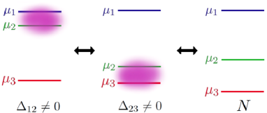
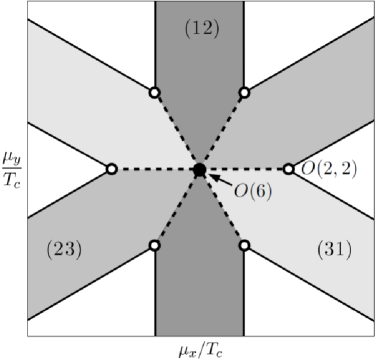
Figure 1: (Color online) Structure of the phase diagram for a constant DOS. Top: SF forms between fermions with the closest chemical potentials, whereas at higher differences the normal state (N) is favored. Bottom: Cut of the SF phase diagram for $T\lesssim T_{c}$ Apart from the special points (full and empty circles) SF order always forms in one of the channels (12), (23) or (31). At the point $\mu_{x}=\mu_{y}=0$ (full circle) the Hamiltonian is $SU(3)$ symmetric, and the transition is described by an $O(6)$ critical point. The first order lines, separating different SF phases terminate in second order critical points with $O(2,2)$ symmetry (empty circles).

Although we also discuss to a certain extent the role of fluctuations in Section V, the bulk of this work consists of a mean-field analysis. Even this is, however, not entirely trivial. In the Hubbard-Stratonovich approach of Refs. HonerkampHofstetterRPA, and Demler, the decoupling of the interaction into ferromagnetic and superfluid parts suffers from a certain degree of arbitrariness.footnote Treating the ferromagnetic and superfluid order parameters at equal footing therefore requires care. Furthermore, at lower temperatures the second order transitions turn into first order transitions, and the free energy develops several inequivalent local minima. To cope with these difficulties, we applied two complementary methods: an equation of motion method, where vertex corrections are systematically neglected, and a Gaussian variational approach. Both approaches are exempt from the arbitrariness of the Hubbard-Stratonovich transformation, account for the interplay between ferromagnetic and superfluid order, and, remarkably, they both result in the same self-consistency equations. However, the Gaussian variational approach goes beyond the equation of motion method in that it also provides an estimate for the mean field free energy, and allows us to locate first order transitions. Since previous works indicate that the Fulde-Ferrell-Larkin-Ovchinnikov (FFLO) phase with spatially varying order parameterFF ; LO appears only in a tiny region of the phase diagram,FFLOExp1 ; FFLOExp2 here we restrict our investigation to spatially homogeneous phases. We shall neither consider Breached Pair (BP) or Sarma phases,Wilczek ; Sarma since these would require fermions of very different masses.

Before we turn to the more detailed presentation of the calculations, let us summarize here our most important results. In the small coupling limit, $T_{c}\ll W$, the phase diagram is expected to become universal for $SU(3)$ symmetrical interactions: it should depend only on the dimensional temperature, $T/T_{c}$, the dimensionless chemical potential shifts, $\delta\mu_{\alpha}/T_{c}$, and the dimensionless particle-hole symmetry breaking, $\tilde{\gamma}\equiv\gamma T_{c}$, defined in terms of the critical temperature $T_{c}$ at the $SU(3)$ symmetrical point, $\mu_{\alpha}\equiv\mu$. Fig. 1 shows the corresponding schematic phase diagram in case of a particle-hole symmetrical situation, $\gamma=0$. The bottom figure shows a finite temperature cut of the phase diagram as a function of the chemical potential differences,

$$\mu_{x} \equiv (\mu_{1}-\mu_{2})/\sqrt{2}\;,$$

$$\mu_{y} \equiv (\mu_{1}+\mu_{2}-2\mu_{3})/\sqrt{6}\;,$$

for a temperature $T$ fixed somewhat below the $SU(3)$ symmetrical transition temperature, $T_{c}$. In the various gray regions two species of the smallest chemical potential difference pair up to form a superfluid (SF) state, while the third species remain gapless. This explains the star-like structure of the phase diagram: superfluid phases appear around regions, where two of the chemical potentials become equal. As we discuss later, the high (”hexagonal”) symmetry of the figure is a direct fingerprint of the $SU(3)$ symmetrical interaction, and a discrete particle hole symmetry. The superfluid state is destroyed, once all chemical potential differences become large compared to the condensation energy (white region). Close to $T_{c}$ the chemical potential driven SF-normal transitions are of second order (black lines), just as in case of a two component mixture.Sarma The transition between different SF phases is, however, always of first order (dashed lines).

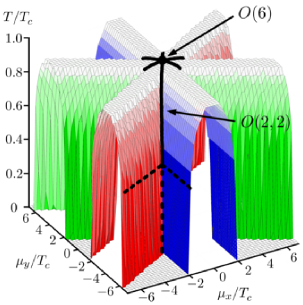
Figure 2: (Color online) Numerically computed SF-N phase boundary as a function of the chemical potentials at constant DOS for $\lambda\rho_{F}=0.1$, and $\gamma=\xi_{F}=0$, corresponding to $T_{c}^{SU(3)}/W=0.0076$. The SF-N transition becomes of first order below a temperature $\widetilde{T}^{\rm\;Sarma}$ (horizontal dashed lines). Vertical lines denote the $O(2,2)$ critical points of second (solid line) and of first order (dashed line).

The phase diagram also exhibits some interesting points of special symmetry. At the point $\mu_{x}=\mu_{y}=0$ the Hamiltonian is $SU(3)$ symmetrical, and correspondingly, the phase transition at $T=T_{c}$ and $\mu_{x}=\mu_{y}=0$ is described by an $O(6)$ theory (the six components corresponding to the real and imaginary parts of the superfluid order parameters). In three dimensions, this symmetry is spontaneously broken for $T<T_{c}$. On the other hand, at the points indicated by white circles in Fig. 1, the competition of two order parameters most likely leads to a so-called $O(2,2)$ critical behavior (see Section V).

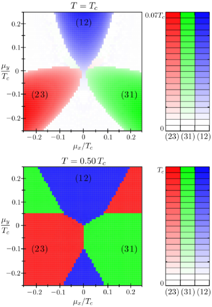
Figure 3: (Color online) Phase diagram in the vicinity of the $SU(3)$ symmetric point in the absence of particle-hole symmetry, $\gamma\neq 0$. The sixfold symmetry of the phase diagram is destroyed. A higher DOS can make SF ordering favorable in a channel not of the smallest chemical potential difference, due to the gain in condensation energy. For the absolute values of the SF order parameters $\Delta_{ij}$ see color code (right). Parameters at the $SU(3)$ symmetric point: $\lambda_{\alpha\neq\beta}\rho_{F}=0.112,\,\gamma W=0.5,\,T_{c}/W=0.011,\xi_{F}/W=0.24$ (half-filling).

Fig. 2 shows the numerically obtained phase diagram in a 3-dimensional plot under the assumption of $SU(3)$ symmetric interaction and particle-hole symmetry ($\gamma=0$). The dome-like structures correspond to superfluid phases with pairing in the $(12)$, $(23)$, and $(31)$ channels. Below the horizontal dashed lines the chemical potential driven phase transitions become of first order, while above these lines they are of second order. These lines are thus the analogues of the critical point identified by Sarma.Sarma The SF-normal transitions on the ”roofs” of the domes belong to the $O(2)$ universality class, while the black solid lines correspond to $O(2,2)$ critical points. Finally, the crossing of the black lines at $\mu_{x}=\mu_{y}=0$ corresponds to an $O(6)$ critical point.

This rich phase diagram is further complicated if one allows for particle-hole symmetry braking, $\gamma\neq 0$.footnote2 On a larger scale, the $\gamma\neq 0$ phase diagram looks quite similar to the $\gamma=0$ phase diagrams, presented in Figs. 1 and 2, however, the structure of the phase diagram changes in the close vicinity of the $SU(3)$ symmetrical point. This is demonstrated in Fig. 3, where the central region of the phase diagram is shown for $T=T_{c}$ and $T=0.5\,T_{c}$. The absence of particle-hole symmetry destroys the hexagonal symmetry of the phase diagram, and leads to a trigonal structure, as predicted by Cherng et al..Demler In this central region a higher DOS, — and thus gain in condensation energy — may make SF ordering favorable in a channel not of the smallest chemical potential difference. This effect is most spectacular at $T=T_{c}$, where by shifting the Fermi energy of two species one can increase the critical temperature, and induce superfluidity (see Fig. 3, top). We remark, however, that in spite of the relatively large particle-hole asymmetry introduced, this central region is typically quite small compared to the rest of the phase diagram, at least for weak couplings, $T_{c}\ll W$. The orientation of the phases is, however, opposite to the one predicted in Ref. Demler, : to obtain the same orientation, we need to flip the sign of the slope of the DOS, and assume a hole-like Fermi surface, $\gamma<0$. We must also add here that the Ginzburg-Landau action of Ref. Demler, is unable to capture the endpoints of the ”trigonal” region, and one must retain higher order terms in the action to account for these (see Section IV).

The rest of the paper is organized as follows: In Section II, we introduce our mean-field methods. We also discuss the symmetries of the order parameters, leading to rather strong constraints on the form of the phase diagram. In Section III, we present our main results on the SF phase diagram, with and without particle-hole symmetry, and compare our findings with results on two component systems. In Section IV we present the numerical Ginzburg-Landau expansion of the free energy around the $SU(3)$ symmetric point, and identify the terms responsible for the main features of the central part of the phase diagram. In Section V we discuss the effect of fluctuations in the special $O(2,2)$ symmetric bicritical points. In Section VI we comment on the experimental realizability of an $SU(3)$ symmetric system. Some of the technical details of our calculations can be found in the Appendices.

II Mean-field calculations

In this section, we first use an imaginary time equation of motion (EOM) method to derive the self-consistency equations for the SF and magnetic order parameters. Then, to address the low temperature regime, where these equations have multiple solutions,Sarma we also develop a Gaussian variational approximation. This approach provides an estimate for the free energy and enables one to locate first order transitions.

II.1 Equation of motion technique

To simplify our notation, let us first introduce the 6 component Nambu spinor field

$$\Phi(x)=\left(\Psi(x),\Psi^{\dagger}(x)\right)^{T}\;.$$

Here we used the compact notation $x=(\mathbf{r},\tau)$ for the space and imaginary time coordinates. The corresponding $6\times 6$ propagator matrix $\mathbf{D}(x_{1},x_{2})\equiv-\langle T_{\tau}\,\Phi(x_{1})\circ\Phi^{\dagger}(x_{2})\rangle$ contains the normal as well as the anomalous Green’s functions of the fields $\Psi_{\alpha}(x)$ and, assuming spatial homogeneity, also obeys $\mathbf{D}(x_{1},x_{2})=\mathbf{D}(x_{1}-x_{2})$. In order to derive equation of motion for the propagators, we start from the imaginary time equation of motion (EOM) of the fields,

$$\partial_{\tau}\Psi_{\alpha}(x)=\left[H,\Psi_{\alpha}(x)\right].$$ (2)

The EOM of the part $-\langle\mathrm{T}_{\tau}\Psi_{\alpha}(x_{1})\Psi^{\dagger}_{\beta}(x_{2})\rangle$ of the propagator follows from Eq. (2), and reads

$$\left(\partial_{\tau_{1}}+\mathcal{H}_{0}(\mathbf{r}_{1})-\mu_{\alpha}\right)\langle\mathrm{T}_{\tau}\Psi_{\alpha}(x_{1})\Psi^{\dagger}_{\beta}(x_{2})\rangle=\delta_{\alpha\beta}\delta_{x_{1}x_{2}}$$ (3)

$$+\sum_{\gamma}2\lambda_{\alpha\gamma}\langle\mathrm{T}_{\tau}\Psi^{\dagger}_{\gamma}(x_{1})\Psi_{\gamma}(x_{1})\Psi_{\alpha}(x_{1})\Psi^{\dagger}_{\beta}(x_{2})\rangle,$$

with $\delta_{x_{1}x_{2}}$ denoting the four dimensional Dirac-delta function. Similar equations hold for the anomalous propagators, $-\langle\mathrm{T}_{\tau}\Psi_{\alpha}(x_{1})\Psi_{\beta}(x_{2})\rangle$ and $-\langle\mathrm{T}_{\tau}\Psi^{\dagger}_{\alpha}(x_{1})\Psi^{\dagger}_{\beta}(x_{2})\rangle$.

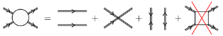
Figure 4: (Color online) Omission of the vertex corrections in the connected four point functions (l.h.s.). Heavy lines denote the full propagators, and the square stands for the vertex contribution.

To make further progress, we simplify the four point functions appearing in these EOMs, by simply neglecting the vertex contribution, as shown in Fig. 4. This approximation is almost equivalent to the usual BCS approximation, however, it goes beyond that, since it allows for the simultaneous appearance of different kinds of order parameters in an unbiased way. Furthermore, even in the simple $SU(2)$ case, it also incorporates, e.g., the renormalization of the Pauli susceptibility at the mean- field level (see Section III.3). With this approximation, the equation of motion become solvable, and the Nambu propagator is found to take the following form in Fourier space

$$\mathbf{D}(i\omega_{n},\mathbf{k})^{-1}=\,i\omega_{n}-\mathbf{B}(\xi_{\mathbf{k}}).$$ (4)

Here $\omega_{n}=(2n+1)\,\pi\,T$ are fermionic Matsubara frequencies and the matrix $\mathbf{B}(\xi)$ is defined as

$$\mathbf{B}(\xi)\equiv\,\begin{pmatrix}\xi-\mathbf{\Lambda}&2\mathbf{\Delta}\\ 2\mathbf{\Delta}^{+}&-\left(\xi-\mathbf{\Lambda}^{*}\right)\end{pmatrix}.$$ (5)

The matrices

$$\Delta_{\alpha\beta}\equiv \,\lambda_{\alpha\beta}d_{\alpha\beta},$$ (6)

$$\Lambda_{\alpha\beta}\equiv \,(\mu_{\alpha}+2\sum_{\gamma}\lambda_{\alpha\gamma}n_{\gamma\gamma})\delta_{\alpha\beta}-2\lambda_{\alpha\beta}n^{*}_{\alpha\beta}$$ (7)

denote the SF order parameterfootnoteOrderParametersConvDifference and the renormalized chemical potential, respectively. They are defined in terms of the matrix of densities $\mathbf{n}$, and that of the anomalous densities $\mathbf{d}$,

$$n_{\alpha\beta}\equiv \langle\Psi_{\alpha}^{\dagger}(x_{1})\Psi_{\beta}(x_{1})\rangle,$$ (8)

$$d_{\alpha\beta}\equiv \langle\Psi_{\alpha}(x_{1})\Psi_{\beta}(x_{1})\rangle.$$ (9)

The matrices $\mathbf{n}$ and $\mathbf{d}$ can be used to describe magnetic and SF ordering, respectively. However, it is more natural to use $\mathbf{\Lambda}$ and $\mathbf{\Delta}$ as order parameters. Note that, according to Eq. (7), magnetic ordering implies a shift in the renormalized chemical potential $\Lambda_{\alpha\beta}$, and this shift can thus also be considered as a magnetic order parameter.

The expectation values Eqs. (8) and (9) are given by the propagator $\mathbf{D}(x_{1}-x_{2})$ at equal times and equal positions, and are thus determined by Eq. (4). Taking the inverse of Eq. (4) and performing the Matsubara summation over the frequencies $\omega_{n}$ we obtain

$$\int_{-W}^{W}\mathrm{d}\xi\,\rho(\xi)\,f\left(\mathbf{B}(\xi)\right)=\begin{pmatrix}\mathbf{n}^{*}&-\mathbf{d}\\ -\mathbf{d}^{+}&-\mathbf{n}+\int\mathrm{d}\xi\,\rho(\xi)\end{pmatrix},$$ (10)

where $\rho(\xi)$ denotes the DOS of $\mathcal{H}_{0}$, and $f$ stands for the Fermi function. Eqs. (5-7) and (10) thus determine self-consistently the order parameters $\mathbf{\Lambda}$ and $\mathbf{\Delta}$. We solve these equations iteratively, starting from random initial conditions, and performing the integrals in Eq. (10) numerically. Notice that $f(\mathbf{B}(\xi))$ is a matrix function, therefore, its evaluation requires numerical diagonalization of the Hermitian matrix $\mathbf{B}(\xi)$ for each value of $\xi$.

We remark that the matrix $\mathbf{B}(\xi)$ in Eq. (5) possesses a symplectic symmetry

$$\begin{pmatrix}\mathbf{0}&\mathbf{1}\\ \mathbf{1}&\mathbf{0}\end{pmatrix}\mathbf{B}\left(\xi\right)\begin{pmatrix}\mathbf{0}&\mathbf{1}\\ \mathbf{1}&\mathbf{0}\end{pmatrix}=-\mathbf{B}^{\mathrm{T}}\left(\xi\right),$$ (11)

since the order parameters $\mathbf{\Delta}$ and $\mathbf{\Lambda}$ are skew-symmetric and Hermitian, respectively. This symmetry makes the eigenvalues of $\mathbf{B}(\xi)$ come in pairs, $(\upsilon,-\upsilon)$, and thus simplifies some of our calculations of the free energy in the next subsection. It is also responsible for the structure of the equal time, equal position propagator in Eq. (10).

II.2 Gaussian variational approach

To investigate the low temperature phase diagram, we employ a variational method. This method consists of finding the best Gaussian approximation to the free energy $F=-T\log\mathcal{Z}$ of the system. As a first step, we express the grand canonical partition function $\mathcal{Z}$ as a functional integral

$$\mathcal{Z}=\int\mathfrak{D}\mathbf{\overline{\psi}}\,\mathfrak{D}\mathbf{\psi}\,e^{-S[\mathbf{\overline{\psi}},\mathbf{\psi}]},$$ (12)

with the action written as $S=S_{0}+S_{\mathrm{int}}$, and the non-interacting and interacting parts defined as

$$S_{0} =-\frac{1}{2}\int\mathrm{d}1\,\mathrm{d}2\;\overline{\phi}(1)\,\mathcal{D}_{0}^{-1}(1,2)\,\phi(2),$$ (13)

$$S_{\mathrm{int}} =-\sum_{\alpha\beta}\lambda_{\alpha\beta}\int\mathrm{d}x\;\overline{\psi}_{\alpha}(x)\overline{\psi}_{\beta}(x)\psi_{\beta}(x)\psi_{\alpha}(x).$$ (14)

Here $\phi=\left(\psi,\overline{\psi}\right)^{T}$ is a Nambu spinor field and we used the notations $"1"=(\mathbf{r}_{1},\tau_{1},\nu_{1})$, and $\int\mathrm{d}1\dots$, to denote the integration over space and imaginary time variables and the summation over Nambu indices ($\nu_{1}=1,\dots,6$) in a compact way. The inverse propagator

$$-\mathcal{D}_{0}^{-1}=\delta_{x_{1}x_{2}}\left(\partial_{\tau_{2}}+\begin{pmatrix}\mathcal{H}_{0}-\hat{\mu}&0\\ 0&-(\mathcal{H}_{0}-\hat{\mu})\end{pmatrix}\right),$$ (15)

contains the single particle Hamiltonian of the free fields, $\mathcal{H}_{0}$, where $\hat{\mu}_{\alpha\beta}=\mu_{\alpha}\,\delta_{\alpha\beta}$ is a $3\times 3$ diagonal matrix containing the chemical potentials.

Our Gaussian approximation of the free energy is based on the standard inequalityFeynman

$$F\leq F_{G}[\mathcal{D}]\equiv-T\log\mathcal{Z}_{\mathcal{D}}+T\langle S-S_{\mathcal{D}}\rangle_{\mathcal{D}}\;.$$ (16)

Here the partition function $\mathcal{Z}_{\mathcal{D}}$ and the average $\langle\dots\rangle_{\mathcal{D}}$ are defined in terms of the Gaussian action

$$S_{\mathcal{D}} \equiv-\frac{1}{2}\int\mathrm{d}1\,\mathrm{d}2\;\overline{\phi}(1)\,\mathcal{D}^{-1}(1,2)\,\phi(2)\;.$$ (17)

$$\mathcal{Z}_{\mathcal{D}} \equiv\int\mathfrak{D}\mathbf{\overline{\psi}}\,\mathfrak{D}\mathbf{\psi}\,e^{-S_{\mathcal{D}}[\mathbf{\overline{\psi}},\mathbf{\psi}]}\;,$$ (18)

$$\langle\dots\rangle_{\mathcal{D}} \equiv\frac{1}{\mathcal{Z}_{D}}\int\mathfrak{D}\mathbf{\overline{\psi}}\,\mathfrak{D}\mathbf{\psi}\;\dots\;e^{-S_{\mathcal{D}}[\mathbf{\overline{\psi}},\mathbf{\psi}]}\;.$$ (19)

Since we do not want to restrict our investigations to actions that can be associated with a Hamiltonian, we do not require $S_{\mathcal{D}}$ to be local. Nevertheless, at the saddle points of $F_{G}$, $S_{\mathcal{D}}$ turns out to be local, and there exists a Hamiltonian associated with it (see Eqs. (22-24) below).

Since the action $S_{\mathcal{D}}$ is quadratic, the propagator matrix of the Nambu fields can be written as

$$\mathcal{D}(1,2)=-\langle\phi(1)\,\overline{\phi}(2)\rangle_{\mathcal{D}}\;,$$ (20)

and expectation values can be evaluated using Wick’s theorem. We remark that the choice (20) automatically fixes a certain ambiguity in the definition of $\mathcal{D}^{-1}$. (For details see Appendix C.) The best Gaussian approximation is given by the minimum of the functional $F_{G}[\mathcal{D}]$, where $F_{G}$ satisfies the saddle point equation

$$\frac{\delta F_{G}}{\delta\mathcal{D}(1,2)}=0.$$ (21)

As is shown in Appendix C, this equation is equivalent to the self-consistency equations (5,6,7) and (10) of the EOM technique, and amounts in $\mathcal{D}^{-1}$ being a local,

$$\mathcal{D}^{-1}(1,2)=\delta(x_{1}-x_{2})\,\mathbf{D}^{-1}(x_{2}).$$ (22)

with the matrix operator on the r.h.s being just the inverse propagator Eq. (4) in real space,

$$-\mathbf{D}^{-1}=\partial_{\tau_{2}}+\begin{pmatrix}\mathcal{H}_{0}(\mathbf{r}_{2})-\mathbf{\Lambda}&2\mathbf{\Delta}\\ 2\mathbf{\Delta}^{+}&-(\mathcal{H}_{0}(\mathbf{r}_{2})-\mathbf{\Lambda}^{*})\end{pmatrix}.$$ (23)

The order parameters $\mathbf{\Lambda}$ and $\mathbf{\Delta}$ are determined by the former equations, Eqs. (6,7).

Thus the Gaussian variational approach is entirely consistent with the EOM method. However, it goes also beyond it, since it enables us to obtain an estimate for the free energy. By Eqs. (22) and (23), to calculate the best approximation $F_{G}$ to the free energy, it is sufficient to consider local actions, for which we can express $S_{\mathcal{D}}$, and thus $F_{G}$, in terms of a Hamiltonian

$$H_{\mathcal{D}}=\frac{1}{2}\int\mathrm{d}^{3}\mathbf{r}\,:\Phi^{\dagger}\begin{pmatrix}\mathcal{H}_{0}-\mathbf{\Lambda}&2\mathbf{\Delta}\\ 2\mathbf{\Delta}^{+}&-\left(\mathcal{H}_{0}-\mathbf{\Lambda}^{*}\right)\end{pmatrix}\Phi:.$$ (24)

Since the functional integrals are, by definition, normal ordered, the Hamiltonian $H_{\mathcal{D}}$ also needs to be normal ordered, as emphasized by the semi-colons in Eq. (24), indicating normal ordering with respect to the vacuum.footnote_normal_order

In this Hamiltonian language, Eq. (16) takes on the form

$$F_{G}(\mathbf{\Lambda},\mathbf{\Delta})=-T\log\mathcal{Z}_{\mathcal{D}}+\langle H-H_{\mathcal{D}}\rangle_{\mathcal{D}}\;,$$ (25)

with $H$ the full Hamiltonian of the system, Eq. (I), and

$$\mathcal{Z}_{\mathcal{D}} = \mathrm{Tr}e^{-\beta H_{\mathcal{D}}},$$ (26)

$$\langle\dots\rangle_{\mathcal{D}} = {\mathrm{Tr}\left(\dots e^{-\beta H_{\mathcal{D}}}\right)}/\mathcal{Z}_{\mathcal{D}}\;.$$ (27)

Notice that $F_{G}(\mathbf{\Lambda},\mathbf{\Delta})$ also depends implicitly on the chemical potentials $\mu_{\alpha}$ and the temperature $T$, and it must be minimized to find the mean field value of the variational parameters, $\mathbf{\Lambda}(\mu_{\alpha},T)$ and $\mathbf{\Delta}(\mu_{\alpha},T)$.

In this Hamiltonian approach, the evaluation of Eq. (25) is straightforward (see Appendix D), and for the free energy density we obtain

$$f_{G}= \,\frac{1}{2}\int\mathrm{d}\xi\,\rho(\xi)\mathrm{Tr}(\xi-\mathbf{\Lambda})$$

$$- \,\frac{T}{2}\int\mathrm{d}\xi\,\rho(\xi)\mathrm{Tr}\log\left(2\cosh\left(\beta\,\mathbf{B}(\xi)/2\right)\right)$$ (28)

$$+ \sum_{\alpha\beta}\left((\mathbf{\Lambda}_{\alpha\beta}-\mu_{\alpha}\delta_{\alpha\beta})\mathbf{n}_{\alpha\beta}+\lambda_{\alpha\beta}\left(|\mathbf{n}_{\alpha\beta}|^{2}-\mathbf{n}_{\alpha\alpha}\mathbf{n}_{\beta\beta}\right)\right)$$

$$+ \sum_{\alpha\beta}\left(\mathbf{\Delta}_{\alpha\beta}\mathbf{d}^{*}_{\alpha\beta}+\mathbf{\Delta}^{*}_{\alpha\beta}\mathbf{d}_{\alpha\beta}-\lambda_{\alpha\beta}|\mathbf{d}_{\alpha\beta}|^{2}\right).$$

Here $\beta=1/T$ is the inverse temperature, the densities $\mathbf{n}$ and $\mathbf{d}$ are determined by Eq. (10), and the matrix $\mathbf{B}(\xi)$ is defined in Eq. (5).

As stated before, at the local minima of the functional $f_{G}$, the order parameters $\mathbf{\Lambda}$ and $\mathbf{\Delta}$ fulfill the EOM self-consistency equations. In our numerical calculations, however, we have not enforced this constraint. Rather, we treated the order parameters as independent and free variables, and used a Monte Carlo method to find the absolute minimum of Eq. (28) in the 15-dimensional space spanned by these order parameters. In the end, we verified numerically that at the minima $\mathbf{\Lambda}$ and $\mathbf{\Delta}$ indeed satisfy the EOM self-consistency equations.

A comparison of the variational Monte Carlo approach and the straightforward solution of the EOM self-consistency equations is presented in Fig. 5. At low temperatures, the EOM becomes unreliable in the vicinity of first order phase boundaries, and finds several possible local minima. The variational Monte Carlo method (with simulated annealing), however, finds the absolute minimum of the free energy, $f_{G}$, and is able to identify the physically relevant solution.

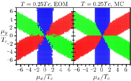
Figure 5: (Color online) Comparison of the EOM and the Gaussian variational methods. Left: At low temperatures the EOM equations have multiple solutions, and become unreliable close to first order phase boundaries. Right: The variational approach combined with a simulated annealing identifies correctly the physically relevant absolute minima of the free energy density, Eq. (28). Parameters used were: $\lambda_{\alpha\neq\beta}\rho_{F}=0.112$, $\gamma W=0.5$, $T_{c}/W=0.011$, and $\xi_{F}/W=0.24$ (half-filling).

II.3 Symmetries

For an $SU(3)$ symmetrical interaction, $\lambda_{\alpha\neq\beta}=\lambda$, the structure of the phase diagram is largely determined by the underlying $SU(3)$ symmetry. In particular, for $\mu_{\alpha}\equiv\mu$ the Hamiltonian is invariant under global $SU(3)$ rotations, $\Psi_{\alpha}(x)\mapsto\sum_{\beta}U_{\alpha\beta}\Psi_{\beta}(x)$, and a global U(1) gauge transformation, $\Psi_{\alpha}(x)\mapsto e^{i\varphi}\,\Psi_{\alpha}(x)$.

The ferromagnetic order parameters $\mathbf{n}$ and $\mathbf{\Lambda}$ are Hermitian. They are invariant under the U(1) gauge transformation, and transform under $SU(3)$ rotations as

$$\mathbf{n}^{\mathrm{T}}\mapsto\mathbf{U}\,\mathbf{n}^{\mathrm{T}}\mathbf{U}^{\dagger},\hskip 12.0pt\mathbf{\Lambda}\mapsto\mathbf{U}\,\mathbf{\Lambda}\mathbf{U}^{\dagger},$$ (29)

which, — after taking out the trivial trace, — is equivalent to the 8-dimensional adjoint representation of $SU(3)$.

The order parameters $\mathbf{d}$ and $\mathbf{\Delta}$ are, on the other hand, skew-symmetric, transform as $\mathbf{d}\mapsto e^{i2\varphi}\,\mathbf{d}$ and $\mathbf{\Delta}\mapsto e^{i2\varphi}\,\mathbf{\Delta}$ under U(1) gauge transformations, and the global $SU(3)$ group transforms them according to

$$\mathbf{d}\mapsto\mathbf{U}\,\mathbf{d}\mathbf{U}^{\mathrm{T}},\hskip 12.0pt\mathbf{\Delta}\mapsto\mathbf{U}\,\mathbf{\Delta}\mathbf{U}^{\mathrm{T}},$$ (30)

which is equivalent to the conjugate representation of $SU(3)$. This can be seen by introducing the 3 component vectors $\underline{d}_{\alpha}=\frac{1}{2}\sum_{\beta\gamma}\epsilon_{\alpha\beta\gamma}d_{\beta\gamma}$ and $\underline{\Delta}=\frac{1}{2}\sum_{\beta\gamma}\epsilon_{\alpha\beta\gamma}\Delta_{\beta\gamma}$ by means of the completely antisymmetric Levi-Civita symbol $\epsilon_{\alpha\beta\gamma}$. In this form Eq. (30) reads

$$\underline{\mathbf{d}}\mapsto\,\mathbf{U}^{*}\underline{\mathbf{d}},\phantom{nn}\underline{\mathbf{\Delta}}\mapsto\mathbf{U}^{*}\underline{\mathbf{\Delta}}\;.$$ (31)

In the special case, $\lambda_{\alpha\neq\beta}=\lambda$ and $\mu_{\alpha}=\mu$, symmetry implies that the Ginzburg-Landau functional must be invariant under the transformations (29) and (30), and the U(1) gauge transformation. The onset of superfluidity, however, spontaneously breaks the $SU(3)\otimes U(1)$ symmetry down to $SU(2)\otimes U(1)$. This spontaneous symmetry breaking is accompanied by the emergence of five Goldstone modes.HonerkampHofstetterRPA

The presence of the chemical potentials, $\hat{\mu}_{\alpha\beta}=\delta_{\alpha\beta}\mu_{\alpha}$, obviously breaks the $SU(3)$ symmetry. However, one has strong symmetry-dictated constraints on the Ginzburg-Landau functional even in this case, and the latter must be invariant with respect to the transformations in Eqs. (29) and (30), provided that $\hat{\mu}$ is also transformed accordingly, $\mathbf{\hat{\mu}}\mapsto\mathbf{U}\,\mathbf{\hat{\mu}}\mathbf{U}^{\dagger}$ (see also Section IV). In addition, even in the presence of chemical potential differences, $SU(3)$ symmetry implies Ward identities,Demler relating four-point expectation values and the ferromagnetic order parameter $\mathbf{n}$ as

$$\left(\mu_{\alpha}-\mu_{\beta}\right)n_{\alpha\beta}=\sum_{\gamma}2\left(\lambda_{\beta\gamma}-\lambda_{\alpha\gamma}\right)\langle{\Psi}^{\dagger}_{\gamma}{\Psi}^{\dagger}_{\alpha}\Psi_{\beta}\Psi_{\gamma}\rangle\;.$$ (32)

From this identity (derived in Appendix A) it follows that $\mathbf{n}$ is diagonal for an $SU(3)$ symmetric interaction. We remark that a similar approximate Ward identity can be derived within the Gaussian variational method (see Appendix B), leading to the same conclusions.

The off-diagonal elements of the chemical potential tensor, $\mathbf{\hat{\mu}}$ describe tunneling between different hyperfine components, and they typically vanish in practical situations. Under these restrictions, allowed $SU(3)$ rotations generate essentially only permutations of the hyperfine labels, $\alpha$, and the corresponding chemical potentials, $\mu_{\alpha}$. On the $(\mu_{x},\mu_{y})$ plane, these permutations translate to $C_{3}$ rotations and reflections, and give a two-dimensional representation of the ${\mathbb{S}}_{3}\sim C_{3v}$ group, implying a triangular symmetry of the phase diagram in this plane (see Fig 3).

In addition to the symmetries discussed above, for an $SU(3)$ symmetrical Hamiltonian, the mean field equations also have a certain particle-hole symmetry if the single particle density of states obeys $\varrho(\xi)=\varrho(-\xi)$, and the chemical potentials are set to a value, $\mu\to\mu_{\rm half}$, such that $\varrho$ is exactly half-filled. Under these conditions we can show (see Appendix E) that the mean field solutions are symmetrical in the sense that for $\delta\mu_{\alpha}\equiv\mu_{\alpha}-\mu_{\rm half}$ and for $\delta\mu_{\alpha}\to-\delta\mu_{\alpha}$ the superfluid and magnetic symmetries are broken in the same channels and the order parameters are also equal apart from signs, global gauge transformations, and conjugation. In this special case, due to the additional permutational symmetry discussed above, the phase diagram exhibits a sixfold $C_{6v}$ symmetry in the $(\delta\mu_{x},\delta\mu_{y})$ plane for traceless chemical potential shifts, $\delta\mu_{1}+\delta\mu_{2}+\delta\mu_{3}=0$, (see Fig. 1.)

This particle-hole symmetry also emerges at the level of the Hamiltonian in certain cases. The half-filled attractive three component Hubbard model on a bipartite lattice

$$H=-t\sum_{\alpha}\sum_{\langle ij\rangle}(a^{\dagger}_{i\alpha}a_{j\alpha}+h.c.)-\frac{U}{2}\sum_{i}(\sum_{\alpha}n_{\alpha}-\frac{3}{2})^{2}\;,$$

e.g., has an exact particle-hole symmetry: it is invariant under the unitary transformation $a_{i\alpha}\leftrightarrow\mathrm{sign}(i)\;a^{\dagger}_{i\alpha}$, with $\mathrm{sign}(i)$ taking values $\pm$ for the two sublattices. Just as the mean field symmetry discussed in the previous paragraph, this exact symmetry relates the order parameters of the symmetry broken phases for $\pm\delta\mu_{\alpha}$. We remark that, on a lattice, for stronger couplings, in addition to the SF/magnetic phases discussed here, other non-trivial phases may emerge (eg. charge density waves or trionic phases).Rapp ; InducedPolarization

Although the particle-hole symmetry discussed here holds only for a single and special chemical potential value, we found that for $T_{c}\ll W$ higher order terms in the Ginzburg-Landau action are only sensitive to the immediate vicinity of the Fermi surface. As a result, particle-hole symmetry becomes an approximate symmetry with a good accuracy, whenever the slope of the single particle density of states vanishes, $\gamma\equiv 0$. For $\mu_{\alpha}\equiv\mu$, $\lambda_{\alpha\neq\beta}\equiv\lambda$, and $\gamma\equiv 0$ we thus recover a phase diagram of hexagonal symmetry within our numerical accuracy (see Fig. 1).

III Mean-field phase diagram

Let us now present the phase diagrams in the weak coupling limit, $T_{c}\ll W$, as obtained numerically, by the EOM and Monte Carlo methods presented in Section II.

III.1 Constant density of states ($\gamma=0$)

As we argued in the Introduction, except for the $SU(3)$ symmetric point, a system of constant DOS always favors the formation of a SF phase in one of the pairing channels (12), (23) and (31), having the smallest chemical potential difference. If the chemical potential difference between the components forming the SF state exceeds a certain limit (known as the Clogston limitClogston_limit at zero temperature in case of two fermionic components), the system goes into the normal phase. This transition can either be of first or of second order, depending on the temperature.Sarma

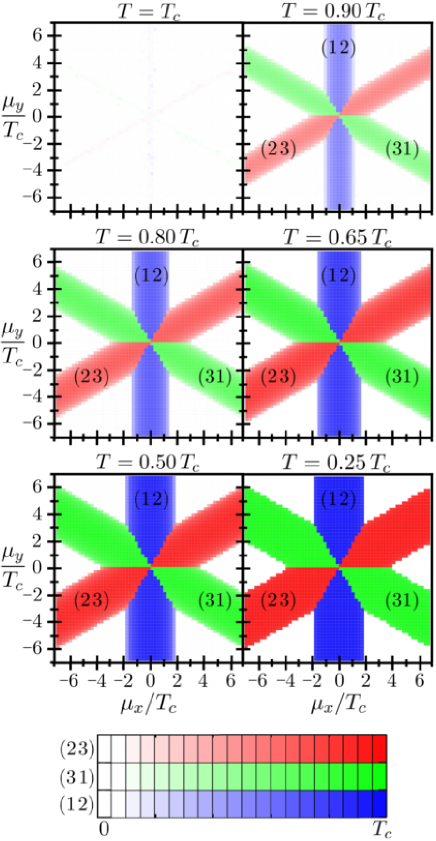
Figure 6: (Color online) Mean-field phase diagrams at constant DOS, $\gamma=0$. Different SF phases are separated by first order lines. At $T=0.25\,T_{c}$ SF-N transitions are of first order, whereas they become of second order for $T>\widetilde{T}^{\rm Sarma}\approx 0.48T_{c}$ (see Section III.3). Absolute values of components of the order parameter $\mathbf{\Delta}$ are given in units of $T_{c}$ (see color code). Parameters at the $SU(3)$ symmetric point: $\lambda_{\alpha\neq\beta}\rho_{F}=0.1$, $T_{c}/W=0.0076$, and $\gamma W=\xi_{F}/W=0$.

Fig. 6 shows the numerically obtained phase diagram at different temperatures. All these cuts have the structure presented in Fig. 1. The hexagonal symmetry of the middle of the phase diagram is related to $SU(3)$ symmetry: it is due to the invariance of the Hamiltonian under the permutations of the fermion species ($\alpha\leftrightarrow\beta$ and $\mu_{\alpha}\leftrightarrow\mu_{\beta}$) and the approximate particle-hole symmetry, as explained in Section II.3. The first order SF-SF transitions appear along lines where the chemical potential differences between two different pairs of fermions become equal. Along some special directions in the $(\mu_{x},\mu_{y})$ plane two out of three fermions have equal chemical potentials, and can form a SF state even far away from the central $SU(3)$ symmetric point. This explains the ray-like structures in Fig. 6. In all other directions the chemical potential differences continue to grow until the system goes into the normal phase at chemical potential differences of the order of the superfluid gap at the $SU(3)$ symmetric point. For $T>\widetilde{T}^{\rm Sarma}\approx 0.48\,T_{c}$ this chemical potential driven SF-normal transition is of second order, however it becomes of first order below $\widetilde{T}^{\rm Sarma}$ (see Section III.3).

III.2 Linear density of states ($\gamma\neq 0$)

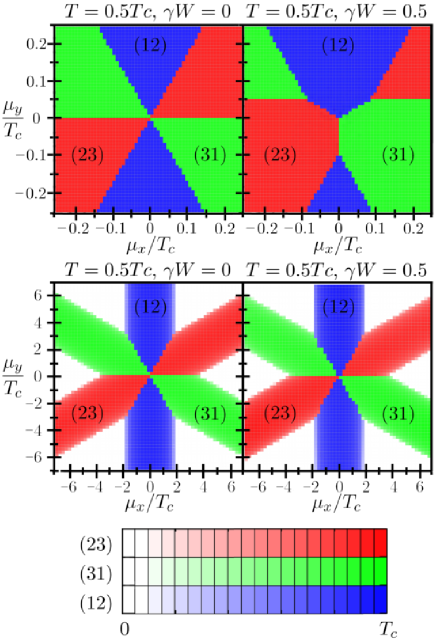
Figure 7: (Color online) Phase diagrams at constant (left) and linear (right) DOS at $T=0.5T_{c}$. Non-zero $\gamma$ deforms the middle of the phase diagram (top right), whereas on the large scale (middle), the phase diagram with constant and linear DOS are almost identical. Parameters at the $SU(3)$ symmetric point: $(\lambda_{\alpha\neq\beta}\rho_{F},\,T_{c}/W,\,\gamma W,\xi_{F}/W)=(0.1,0.0076,0,0)$ in the left and $(0.112,0.011,0.5,0.24)$ in the right figures.

In case of a non-constant DOS ($\gamma\neq 0$), particle-hole symmetry is broken at the Fermi surface, even at the $SU(3)$ symmetric point. At a first glance, the phase diagram is only slightly different from the $\gamma=0$ case, however, at a closer look qualitative differences can be discovered (see bottom and top parts of Fig. 7). For $\gamma\neq 0$ the SF state not necessarily forms in the channel with the smallest chemical potential difference. The reason is that the gap is exponentially sensitive to the DOS. As a result, it may be favorable to form an SF state in channels, where the DOS is larger at the chemical potential, even at the expense of Zeeman energy (chemical potential) loss. This mechanism is driven by the derivative of the DOS $\gamma$, and changes the phase diagram close to the $SU(3)$ symmetric point. Here the phase diagram has only three-fold symmetry, corresponding to ’color’ permutations, and superfluidity forms in channels of the largest density of states. At higher values of the chemical potential, however, the phase diagram remains essentially unaltered, and is almost identical to that of constant density of states.

These results are similar to the predictions of Ref. Demler, , however, the phase structure differs somewhat, and the direction of the phase diagram of Ref. Demler, seems to be flipped. We verified, that both the variational calculation and the equation of motion method yield consistently the phase diagram presented here, which we can also reproduce by the Ginzburg-Landau approach, presented in Section IV. As we discuss there, the Ginzburg-Landau action of Ref. Demler, cannot produce the six-fold symmetric structure of the overall phase diagram, and one needs to keep higher order terms to recover it.

The previously discussed region of three-fold symmetry is, however, usually small compared to the overall scale of the phase diagram. For the parameters of the left figures in Fig. 7, e.g., $T_{c}/W=0.011$, and a relatively steep density of states with $\gamma W=0.5$, the three-fold symmetric region is present only for $|\mu_{x}|,|\mu_{y}|<0.1\;T_{c}$, while the overall scale of the phase diagram is about $\sim 3\;T_{c}$. The relative size of this central region increases for larger interaction strengths, and for $T_{c}/W=0.105$ and $\gamma W=0.5$ we find, e.g., that the central triangular region extends to $|\mu_{x}|,|\mu_{y}|<0.25\;T_{c}$. The size of the central triangular region seems to scale roughly as $\sim\sqrt{\gamma T_{c}}$.

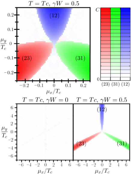
Figure 8: (Color online) Phase diagrams at $T=T_{c}$ with constant (bottom left) and linear ($\gamma W=0.5$) DOS (top left and bottom right). For linear DOS the SF-N critical temperature can exceed $T_{c}$ of the $SU(3)$ symmetric point, whereas for $\gamma=0$, the SF phase disappears everywhere above $T_{c}$. The largest values of the color scales correspond to $|\Delta_{\alpha\beta}|=0.07T_{c}$ (top left), and $|\Delta_{\alpha\beta}|=T_{c}$ (bottom left and right). Parameters at the $SU(3)$ symmetric point are $(\lambda_{\alpha\neq\beta}\rho_{F},\,T_{c}/W,\,\gamma W,\xi_{F}/W)=(0.1,0.0076,0,0)$ in the bottom left and $(0.112,0.011,0.5,0.24)$ in the top left and bottom right figures.

In Fig. 8 we confirm the predictions of Ref. Demler, , that breaking the $SU(3)$ symmetry by the chemical potential can indeed lead to the appearance of superfluidity. Again, this is simply related to the fact, that the superfluid transition temperature is exponentially sensitive to the DOS at the Fermi energy. At the $SU(3)$ critical temperature $T_{c}$, superfluidity appears only in small regions of the phase diagram, around the lines where two of the three fermion species have equal chemical potentials. These regions lie on that side of the $SU(3)$ symmetric point, where the particles of the closest chemical potentials have higher DOS at the Fermi energy than the third one. We remark that the expansion of the free energy up to third order in the order parameters can not recover this structure precisely, and here the phase diagram is significantly different from the phase diagram of Ref. Demler, .

III.3 Two component superfluidity

It is instructive to compare our mean-field theory with results obtained for two component systems. As first noticed by Sarma,Sarma for two component systems the Zeeman field-induced SF-N transition becomes of first order below the temperature ${T}^{\rm Sarma}$, and above the chemical potential difference ${\mu}_{x}^{\rm Sarma}=({\mu}_{1}^{\rm Sarma}-{\mu}_{2}^{\rm Sarma})/\sqrt{2}$. Sarma also determined the mean-field values of this critical point (Sarma point), and obtained

$${T}^{\rm Sarma}=\,0.58\,{T}_{c}\;,\phantom{nnn}{\mu}_{x}^{\rm Sarma}=\,1.5\,{T}_{c}\;,$$ (33)

with ${T}_{c}$ the critical temperature at $\mu_{x}=0$. He also determined the critical chemical potential difference at zero temperature, known as the Clogston limitClogston_limit ,

$${\mu}^{\rm Clog}_{x}=2\,{\Delta}(T=0)=1.764\,T_{c}\;,$$ (34)

with ${\Delta}$ denoting the SF order parameter.

The three component system exhibits a two component behavior in regimes where the chemical potential of two species remains close, e.g. $|\mu_{1}-\mu_{2}|\sim T_{c}$, while that of the third component is very far from them ($|\mu_{3}|\gg T_{c}$). To investigate this limit, we fixed $\mu_{y}=5T_{c}$, and varied $\mu_{x}$, along the solid line shown in the top left panel of Fig. 9. The corresponding SF phase diagram displays features similar to those predicted by Sarma. At $T=0$ temperature, the absolute value of the SF order parameter is independent of $\mu_{x}$ in the superfluid phase, and its magnitude agrees with the BCS result, $\Delta(T=0)=0.882\;T_{c}^{(*)}$, with $T_{c}^{(*)}$ being the critical temperature at $\mu_{x}=0$.footnoteTcStar The critical value of $\mu_{x}$ (Clogston limit), however, shows significant deviations compared to Eq. (34). For a coupling $\tilde{\lambda}\equiv\lambda\rho_{F}=0.1$, e.g., we find both for a two and for a three component system

$$\mu^{\rm Clog}_{x}\to\left.\widetilde{\mu}^{\rm Clog}_{x}\right|_{\tilde{\lambda}=0.1}=2.19\,\Delta(T=0)=1.93\,T_{c}^{(*)}\;.$$ (35)

For $T_{c}\ll W$, the prefactor was found to be approximately independent of the value of $\mu_{y}$ and particle-hole symmetry breaking parameter, $\tilde{\gamma}$. The difference between Eq. (35) and Clogston’s result is due to the inclusion of magnetic degrees of freedom in the free energy density, Eq. (28), which accounts for interaction-related contributions to the Pauli susceptibility, $\chi\sim\rho_{F}$, neglected in Sarma’s work.Sarma These susceptibility contributions are proportional to $\lambda_{\alpha\beta}\rho_{F}^{2}$, and therefore result in a correction to the magnetic energy of relative size $\sim\lambda_{12}\rho_{F}$, in rough agreement with the numerically observed shift of $\mu^{\rm Clog}_{x}$. It is easy to understand this difference on physical grounds: In the SF state (12), the densities $n_{11}$ and $n_{22}$ are exactly equal at $T=0$, while in the normal state they shift according to the chemical potential difference. The interaction is, however, repulsive in the magnetic channel. Consequently, the (magnetized) normal state becomes less favorable, and $\mu^{\rm Clog}_{x}$ shifts upwards.

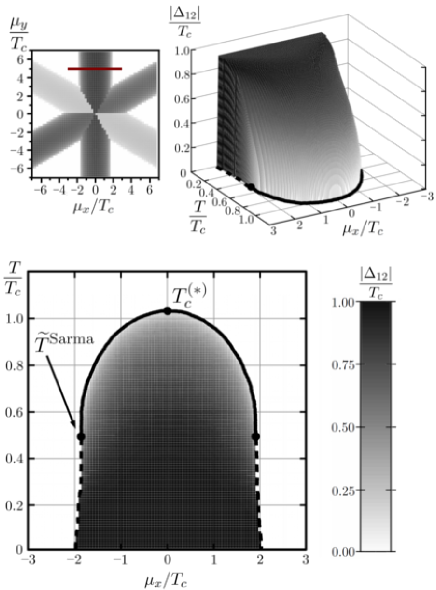
Figure 9: (Color online) SF phase diagram (top right and bottom) at linear DOS ($\gamma W=0.5$), with $\mu_{y}=5T_{c}$ kept constant, as indicated by the solid line in the top left figure. The SF-N transition becomes from second order (solid line) to first order (dashed line) below the temperature $\widetilde{T}^{\rm Sarma}=0.48\,T_{c}^{(*)}$, and chemical potential difference $\widetilde{\mu_{x}}^{\rm Sarma}=1.842\,T_{c}^{(*)}$, with $T_{c}^{(*)}=1.027\,T_{c}$ the critical temperature at $\mu_{x}=0$ and $\mu_{y}=5T_{c}$. Parameters at the $SU(3)$ symmetric point were: $\lambda_{\alpha\neq\beta}\rho_{F}=0.1,\gamma W=0.5,T_{c}/W=0.0076,\xi_{F}=0$.

Locating numerically the Sarma point we also find that it is shifted compared to Eq. (33),

$${T}^{\rm Sarma}\to\left.\widetilde{T}^{\rm\;Sarma}\right|_{\tilde{\lambda}=0.1}= \,0.48\,T_{c}^{(*)}\;,$$ (36)

$${\mu}_{x}^{\rm Sarma}\to\left.\widetilde{\mu}_{x}^{\rm\;Sarma}\right|_{\tilde{\lambda}=0.1}= \,1.842\,T_{c}^{(*)}\;,$$ (37)

again, approximately independently from the value of $\gamma$. These results and Eq. (35) demonstrate that the positions of the Sarma point and the Clogston point, Eq. (34) can significantly deviate from their standard BCS values due to interaction effects. Furthermore, their independence from the particular value of $\gamma$ shows that, at least for $T_{c}\ll W$, particle-hole symmetry breaking does not have a significant effect on the SF phases in the regime where the chemical potentials are far from the $SU(3)$ symmetric point.

In the SF state, the SF species are bound together, and the condensate itself cannot be polarized. This has an experimentally important manifestation at the SF-N transition, where a sudden shift appears in the densities at the phase boundary, as presented in Fig. 10. At zero temperature, the densities in the SF channel are equal, and their value does not depend on the chemical potential difference, whereas at the SF-N transition, a difference in the densities sets in. At temperatures below $\widetilde{T}^{\rm\;Sarma}$, the SF-N transition is of first order, and the densities jump discontinuously on the phase boundary. In Fig. 10 this amounts to a $\sim 1\%$ jump in the densities. In the strongly interacting regime, however, the jump is expected to take much higher values, similar to two component systems.DensityJumpExp

Let us close this section by investigating the effect of SF transition on the third, normal component. Indeed, in the presence particle-hole symmetry breaking, the SF order parameter couples directly to the magnetization, and should shift the density of the third component. Fig. 10 shows this effect for a linear DOS in the weak coupling limit. We find that the shift in the density of the third component is only of the order of $0.01\%$ for $T_{c}/W=0.0076$, however, for larger ratios, $T_{c}/W=0.1$ (but the same $\gamma$) it reaches values of the order of $1\%$, indicating that this effect may be measurable in the strong coupling regime.

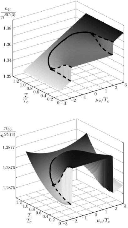
Figure 10: (Color online) Interplay between superfluidity and magnetism in the SF channels, $\alpha=1,2$ (top), and for the third, normal component (bottom), for linear DOS ($\gamma W=0.5$), with $\mu_{y}=5T_{c}$ kept constant. The shift of the densities along the SF-N phase boundary is smooth for $T>\widetilde{T}^{\rm\;Sarma}$ (solid line), and discontinuous for $T<\widetilde{T}^{\rm\;Sarma}$ (dashed line). The density jump of the third component is much smaller than that of the SF components. [See also Fig. 9.] Parameters at the $SU(3)$ symmetric point: $\lambda_{\alpha\neq\beta}\rho_{F}=0.1,\gamma W=0.5,T_{c}/W=0.0076,\xi_{F}=0$.

IV Ginzburg-Landau action

In this section, we focus on the central region of the phase diagram, and construct a Ginzburg-Landau (GL) expansion of the free energy (28) around the $SU(3)$-symmetric point, $\mu_{x}=\mu_{y}=0$ for $T\approx T_{c}$. Throughout this section, we assume a perfectly $SU(3)$ symmetrical interaction, $\lambda_{\alpha\neq\beta}=\lambda$. While the form of the Ginzburg-Landau functional is dictated by symmetry, the coefficients of the various terms depend on the microscopic parameters. We shall give approximate expressions for them, as obtained through a numerical analysis of Eq. (28).

In the weak coupling limit, the dimensionless free energy density,

$$\widetilde{f}_{G}\equiv f_{G}/(\rho_{F}T_{c}^{2})\;,$$

can only depend on a few dimensionless physical parameters: the dimensionless interaction $\widetilde{\lambda}\equiv\rho_{F}\lambda$, the dimensionless slope of the DOS at the Fermi energy $\widetilde{\gamma}\equiv\gamma T_{c}$, the reduced temperature $t\equiv(T-T_{c})/T_{c}$, and the dimensionless chemical potential differences $\delta\widetilde{\mu}=(\mu-\mu^{SU(3)})/T_{c}$, with $\mu^{SU(3)}$ denoting the chemical potential at the $SU(3)$ symmetric point.footnote3 Most importantly, however, $\widetilde{f}_{G}$ is a functional of the dimensionless order parameters,

$$\widetilde{\mathbf{\Delta}}\equiv\mathbf{\Delta}/T_{c}\;,\phantom{nn}\delta\widetilde{\mathbf{\Lambda}}\equiv(\mathbf{\Lambda}-\mathbf{\Lambda}^{SU(3)})/T_{c}\,,$$ (38)

with $\mathbf{\Lambda}^{SU(3)}$ denoting the renormalized chemical potential at the $SU(3)$ symmetric point.

The expansion of the free energy contains only $SU(3)$ invariant terms and can therefore be expanded asDemler

$$\widetilde{f}_{G} =A_{1}\;\mathrm{Tr}(\widetilde{\mathbf{\Delta}}\widetilde{\mathbf{\Delta}}^{+})+A_{2}\,\mathrm{Tr}((\widetilde{\mathbf{\Delta}}\widetilde{\mathbf{\Delta}}^{+})^{2})$$ (39)

$$+\,B_{1}\,\mathrm{Tr}(\delta\widetilde{\mathbf{\Lambda}}^{2})+B_{2}\,\mathrm{Tr}(\delta\widetilde{\mathbf{\Lambda}})^{2}+B_{3}\,\mathrm{Tr}(\delta\widetilde{\mathbf{\mu}}\;\delta\widetilde{\mathbf{\Lambda}})$$

$$+C_{1}\,\mathrm{Tr}(\delta\widetilde{\mathbf{\Lambda}}\widetilde{\mathbf{\Delta}}\widetilde{\mathbf{\Delta}}^{+})+C_{2}\,\mathrm{Tr}(\delta\widetilde{\mathbf{\Lambda}})\mathrm{Tr}(\widetilde{\mathbf{\Delta}}\widetilde{\mathbf{\Delta}}^{+})$$

$$+C_{3}\,\mathrm{Tr}(\delta\widetilde{\mathbf{\mu}}\widetilde{\mathbf{\Delta}}\widetilde{\mathbf{\Delta}}^{+})+\dots.$$

The 8 coefficients appearing in this expansion are all functions of $\widetilde{\lambda}$, $t$, and $\widetilde{\gamma}$. We determined them by fitting the free energy Eq. (28) numerically, and found that the expressions in Table 1 give a good estimate for these parameters.footnote4 At the minima of the free energy functional above we have $\delta\widetilde{\mathbf{\Lambda}}\propto\delta\widetilde{\mathbf{\mu}}$ and $\widetilde{\mathbf{\Delta}}\propto\sqrt{t}$. Therefore, the expansion above contains all terms up to $\mathcal{O}(t^{2},\delta\widetilde{\mu}\,t,\delta\widetilde{\mu}^{2})$.

The superfluid phase transition is driven by the term, $A_{1}(t,\widetilde{\lambda})$, which changes sign at the $SU(3)$ point. All other coefficients are approximately constant close to the phase transition. The terms $\sim B_{i}$ describe the ferromagnetic order parameter, and its response to the external ”magnetic field”, $\widetilde{\mu}$. The most interesting terms are the ones proportional to the coefficients $C_{i}$: these describe the coupling between the SF order parameter and the magnetization (or chemical potential differences), and they are responsible for the three-fold symmetric structure in the central region of the phase diagram (see Fig. 7). The terms $C_{1}$ and $C_{2}$ couple the superfluid and magnetic order parameters, and produce the density shift of the normal component at the onset of superfluidity. Notice that all these terms are found to be proportional to the dimensionless particle-hole symmetry breaking parameter, $\widetilde{\gamma}$.

parameter	approximate expression
$A_{1}$	$2.00\;t+\dots$
$A_{2}$	$0.40-1.20\,t+\dots$
$B_{1}$	$0.5000+1.000\,\widetilde{\lambda}+\dots$
$B_{2}$	$-1.000\,\widetilde{\lambda}+\dots$
$B_{3}$	$-1.000+\dots$
$C_{1}$	$1.25\,\widetilde{\gamma}+\dots$
$C_{2}$	$-1.22\,\widetilde{\gamma}+\dots$
$C_{3}$	$-0.62\,\widetilde{\gamma}/{\widetilde{\lambda}}+\dots$

Table 1: Approximate expressions of the Ginzburg-Landau coefficients in Eq. (39). The dimensionless parameters are $\widetilde{\lambda}\equiv\rho_{F}\lambda$, $\widetilde{\gamma}\equiv\gamma T_{c}$, and $t\equiv(T-T_{c})/T_{c}$.

While the third order expansion, (39) accounts for the central regions on the right panels of Fig. 7, it does not recover the sixfold symmetric structure that dominates the phase diagram at larger chemical potential differences. This is obvious, since the terms $C_{1},C_{2}$ and $C_{3}$ are odd under the particle-hole transformation, $\delta\widetilde{\mu}\leftrightarrow-\delta\widetilde{\mu},\delta\widetilde{\mathbf{\Lambda}}\leftrightarrow-\delta\widetilde{\mathbf{\Lambda}}^{*}$, and are proportional to $\gamma$, while the hexagonal structure is even under particle-hole transformation, and already appears for $\gamma=0$. The ”hexagonal” structure must therefore be controlled by higher order terms, containing even degree polynomials of $\delta\widetilde{\mu}$ and $\delta\widetilde{\mathbf{\Lambda}}$, coupled to the SF order parameter. Unfortunately, the number of such terms is huge, and is next to impossible to determine all of them and their corresponding GL coefficients accurately. However, observing that the ferromagnetic response is always small, we can just focus on the SF order parameter. At a formal level, this can be done by minimizing the free energy functional $\tilde{f}_{G}$ in $\delta\widetilde{\mathbf{\Lambda}}$ for any fixed $\delta\widetilde{\mathbf{\mu}}$ and $\widetilde{\mathbf{\Delta}}$, and thus defining

$${\widehat{f}}_{G}(\delta\widetilde{\mathbf{\mu}},\delta\widetilde{\mathbf{\Delta}})\equiv\widetilde{f}_{G}(\delta\widetilde{\mathbf{\mu}},\delta\widetilde{\mathbf{\Delta}},\delta\widetilde{\mathbf{\Lambda}}_{\rm min}(\delta\widetilde{\mathbf{\mu}},\delta\widetilde{\mathbf{\Delta}}))\;.$$

The form of this GL functional is also dictated by symmetry, and it can also be expanded in $\delta\widetilde{\mathbf{\mu}}$ and $\delta\widetilde{\mathbf{\Delta}}$. Up to $\mathcal{O}(t^{2},\delta\widetilde{\mu}^{2}\,t)$ it readsfootnote4

$${\widehat{f}_{G}} =a_{1}\,\mathrm{Tr}(\widetilde{\mathbf{\Delta}}\widetilde{\mathbf{\Delta}}^{+})+a_{2}\,\mathrm{Tr}((\widetilde{\mathbf{\Delta}}\widetilde{\mathbf{\Delta}}^{+})^{2})$$

$$+b\,\mathrm{Tr}(\delta\widetilde{\mathbf{\mu}}\widetilde{\mathbf{\Delta}}\widetilde{\mathbf{\Delta}}^{+})+c_{1}\,\mathrm{Tr}(\delta\widetilde{\mathbf{\mu}}^{2}\widetilde{\mathbf{\Delta}}\widetilde{\mathbf{\Delta}}^{+})$$ (40)

$$+c_{2}\,\mathrm{Tr}(\delta\widetilde{\mathbf{\mu}}\widetilde{\mathbf{\Delta}}\delta\widetilde{\mathbf{\mu}}\widetilde{\mathbf{\Delta}}^{+})+\dots.$$

The approximate values of the numerically obtained coefficients are enumerated in Table 2.

Minimization of Eq. (40) yields the correct structure of the phase diagram in the vicinity of the $SU(3)$ symmetric point, and accounts for the competition between the odd ($b,\dots$) and even ($c_{1},c_{2},\dots$) order couplings. We also checked that it determines correctly the absolute value of the SF order parameter in the weak coupling regime $T_{c}/W<0.1$ at temperatures $0.9T_{c}<T<T_{c}$. However, the locations of the triple points at the interface of the threefold and approximately sixfold symmetric structures in Fig. 7 are reproduced only with an error of about $50\%$. Although this error is very large, it is also natural, since on the scale of this structure, the chemical potential difference is of the order of $\delta\widetilde{\mu}\approx 0.2$. Therefore $\delta\widetilde{\mu}$ cannot be considered as a small parameter here, and higher order terms in the expansion (40) shift the phase boundaries significantly.

parameter	approximate expression
$a_{1}$	$2.0\;t+\dots$
$a_{2}$	$0.40-1.2\,t+\dots$
$b$	$\left(3.2\,t-0.083/\widetilde{\lambda}^{2}\right)\,\widetilde{\gamma}+\dots$
$c_{1}$	$0.125-0.29\,\widetilde{\lambda}-0.13\,t+\dots$
$c_{2}$	$-0.115+0.27\,\widetilde{\lambda}+0.12\,t+\dots$

Table 2: (Color online) Approximate expressions of the Ginzburg-Landau coefficients in Eq. (40). The dimensionless parameters are $\widetilde{\lambda}\equiv\rho_{F}\lambda$, $\widetilde{\gamma}\equiv\gamma T_{c}$, and $t\equiv(T-T_{c})/T_{c}$.

V Beyond mean-field

In the discussion presented so far we restricted ourselves to a mean-field approach, and neglected fluctuations. Fluctuations, however, not only reduce somewhat the transition temperatures and fields, but they also change the universality class and thus the critical exponents of the transition. In ordinary superfluids, such fluctuation effects are typically hard to observe, however, in cold atomic systems one can reach the strong coupling regime, and therefore a non-trivial critical behavior may be observable.KT_experiment

First, let us discuss the central $SU(3)$ symmetrical point of the phase diagram, $\mu_{x}=\mu_{y}=0$. At this point only the first two terms of the GL action (40) survive for an $SU(3)$ symmetrical interaction. These terms as well as the gradient term, ${\mathrm{T}r}\{\partial_{\bf r}{\mathbf{\Delta}}\cdot\partial_{\bf r}{\mathbf{\Delta}}^{+}\}$ have an increased O(6) symmetry with respect to $SU(3)$,footnote4 with the real and imaginary parts of the independent components of $\mathbf{\Delta}$ forming a six component real vector. Since higher order terms are irrelevant in the renormalization group (RG) sense, the $\mu_{x}=\mu_{y}=0$ transition is described by the O(6) critical theory. Thus the correlation length diverges as $\xi\sim|T-T_{c}|^{-\nu_{O(6)}}$, while the order parameter scales as $\langle\mathbf{\Delta}\rangle\sim|T-T_{c}|^{\beta_{O(6)}}$. For $d=3$ dimensions, the critical exponents are known from $\epsilon$ expansions,O(n)ExponentsEpsilon $1/n$ expansions,O(n)Exponents1N as well as from high-temperature expansions,O(6)ExponentsHT and Monte-Carlo simulations,O(6)ExponentsMC giving similar results,

$$\nu_{O(6)}^{3D}\approx 0.80,\quad\beta_{O(6)}^{3D}\approx 0.41\;.$$

In two dimensions, on the other hand, fluctuations suppress the phase transition at the SU(3)-symmetrical point, $T_{c}^{2D}\to 0$,Cardy which thus becomes a quantum critical point.

For generic values of $\mu_{x},\mu_{y}\neq 0$, only one superfluid channel dominates the phase transition, which is therefore described by the XY model. In $d=3$ dimension the corresponding critical exponents are given byXYExponents

$$\nu_{XY}^{3D} \approx 0.67,\quad\beta_{XY}^{3D}\approx 0.35,$$ (41)

while in $d=2$ dimension the transition is of Kosterlitz-Thouless type.KTpaper

Interesting critical behavior emerges in the vicinity of the bicritical lines of Fig. 2. Along these lines, two components of the matrix ${\mathbf{\Delta}}$, e.g. $\Delta_{13}$ and $\Delta_{23}$ compete with each-other to form the superfluid. These can be grouped into a real four component vector, $\varphi=(\mathrm{Re}\Delta_{23},\mathrm{Im}\Delta_{23},\mathrm{Re}\Delta_{13},\mathrm{Im}\Delta_{13})$. Fermion number conservation implies that the effective action must be invariant under global phase transformations, $\Delta_{ij}\to e^{i\phi_{ij}}\Delta_{ij}$, which translates to an $O(2)\times O(2)$ symmetry in terms of the field $\varphi$. Up to fourth order, the most general effective Hamiltonian can be written asfootnote6

$$H_{LW}= \int\mathrm{d}^{d}x\,\left[\frac{1}{2}(\nabla\varphi)^{2}+t_{+}\varphi^{2}+t_{-}\varphi\mathbf{\Pi}\varphi\right.$$ (42)

$$+ \left.u(\varphi^{2})^{2}+v(\varphi\mathbf{\Pi}\varphi)^{2}+w\varphi^{2}(\varphi\mathbf{\Pi}\varphi)+\dots\right],$$

where the terms breaking the $O(4)$ symmetry were written in terms of the matrix

$$\mathbf{\Pi}=\begin{pmatrix}1&&&\\ &1&&\\ &&-1&\\ &&&-1\end{pmatrix}.$$ (43)

In the absence of the terms $t_{-}$ and $w$, this action has an additional $\mathbb{Z}_{2}$ symmetry, $\Delta_{13}\leftrightarrow\Delta_{23}$, leading to a $O(2,2)=(O(2)\times O(2))\rtimes\mathbb{Z}_{2}$ symmetry of the free energy functional. In the presence of particle-hole symmetry, one can show that at the boundary of the two superfluid phases the $\mathbb{Z}_{2}$ violating terms vanish: $t_{-}=w=0$. In general, however, the simultaneous vanishing of $t_{-}$ and $w$ is not guaranteed. Nevertheless, already leading order $\epsilon$ expansion indicatesEpsilon_intro2 that the coupling $w$ is irrelevant at the phase transition, $t_{\pm}\to 0$. Thus the $\mathbb{Z}_{2}$ symmetry is apparently restored at the transition, and the critical state must be described by the $O(2,2)$ symmetrical functional with $t_{-},w\to 0$.

The $O(2,2)$ functional (42) with $t_{-},w\to 0$ thus describes the phase transition at all bicritical endpoints where two superfluid phases meet (white circles in Fig. 11). Notice that the structure of the phase diagram changes close to $T_{c}$, and the six $O(2,2)$ points, – characteristic at lower temperatures, – pairwise merge into three $O(2,2)$ points above a tricritical temperature, $T^{\mathrm{tri}}$, as also shown in Fig. 11).

The second order terms $t_{+}$ and $t_{-}$ trigger the SF-N and SF-SF transitions, respectively, and scale as

$$t_{+}\propto \,\delta\mu_{\parallel},$$ (44)

$$t_{-}\propto \,\delta\mu_{\perp},$$ (45)

for small chemical potential shifts parallel ($\delta\mu_{\parallel}$) and perpendicular ($\delta\mu_{\perp}$) to the SF-SF phase boundary.

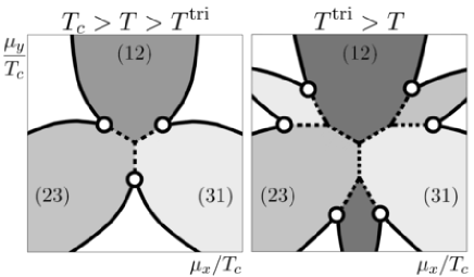
Figure 11: (Color online) Schematic picture of the position of the $O(2,2)$ points (empty circles) in case of linear DOS. At the temperature $T^{\mathrm{tri}}$ below which the triple points appear, from each $O(2,2)$ bicritical line (left) two new bicritical lines of the same universality class branch out (right). The branching points are multicritical. SF-SF transitions are of first (dashed lines), whereas SF-N transitions are of second order (solid lines).

The model (42) has been studied extensively,Epsilon_intro ; Epsilon_intro2 typically in the framework of the more general $n\cdot m$ component models.DombGreen Despite the extensive effort, the stability of its various fixed points is still debated. Systematic $\epsilon$ expansion yields three non-trivial fixed points with $t^{*}_{-}=w^{*}=0$, which could potentially describe the critical state: (a) an $O(4)$ Heisenberg fixed point with $u^{*}>0$ and $v^{*}=w^{*}=0$ (b) a decoupled fixed point (DFP) ($u^{*}=v^{*},w^{*}=0$), where the two superfluid components are described by two independent XY theories, and (c) a mixed (or biconical) fixed point (MFP) with $u^{*}\neq v^{*}$ and $w^{*}=0$.

For small values of $\epsilon=4-d$, $\epsilon$ expansion yields the picture shown in Fig. 12, predicting that the mixed fixed point (MFP) describes the phase transition along the $O(2,2)$ critical line. However, already in second order in $\epsilon$,Epsilon_second_order the fixed point structure changes completely as one approaches the physical value, $\epsilon=1$, and even the results of six loop $\epsilon$ expansion remain completely inconclusive regarding the stability of the fixed points.Epsilon_summary1 Non-perturbative arguments, on the other hand, seem to support that the rather boring decoupled fixed point (DFP) describes the critical state.Epsilon_summary1 ; Epsilon_summary2 ; Epsilon_non_pert

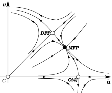
Figure 12: (Color online) Schematic picture of the $\mathcal{O}(\epsilon^{2})$ RG flows in the $(u,v)$ plane, with $t_{-}=w=0$, for $\epsilon<5/7$. For $\epsilon\rightarrow 1$ the fixed point structure changes, and the $\epsilon$ expansion is inconclusive.

The universality class of the fixed point has considerable impact on the phase diagram. The ratio of the critical exponents $y_{\pm}$ associated with the terms $t_{\pm}$ determine e.g. the shape of the SF-N phase boundary in the vicinity of the bicritical point. Standard cross-over scaling argumentsCardy lead to the conclusion, e.g., that the specific heat diverges in the vicinity of the SF-N transition line as

$$c_{v}(t_{+})\propto\left|t_{+}-C(t_{-})\right|^{-\alpha_{\rm XY}},$$ (46)

where $\alpha_{\rm XY}$ denotes the specific heat exponent of the XY model, and the phase boundary is determined by the function $C(t_{-})$

$$C(t_{-})\propto|t_{-}|^{y_{+}/y_{-}}.$$ (47)

Since the critical exponents $y_{{\pm}}$ are different for the two possible stable fixed points even to first order in $\epsilon$,

$$y_{{+}}^{\rm MFP} = 2-\epsilon/2+\dots,\quad y_{{-}}^{\rm MFP}=2-\epsilon/6+\dots,$$ (48)

$$\quad y_{{\pm}}^{\rm DFP}=2-\frac{2}{5}\epsilon+\dots,$$

the shape of the phase boundary will be different in the two cases. Notice that since the DFP describes two independent $XY$ models, its exponents $y^{\rm DFP}_{\pm}$ will be equal to all orders in $\epsilon$, implying that the SF-N boundaries start linearly at the bicritical point. For the MFP, on the other hand, $y_{{+}}^{\rm MFP}<y_{{-}}^{\rm MFP}$, and the SF-N boundary has a universal exponent in the vicinity of the $O(2,2)$ point, as shown in Fig. 13. This difference in the shape of the phase boundary provides a clear fingerprint of the universality class of the transition.

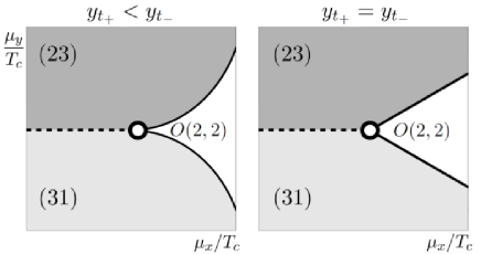
Figure 13: (Color online) Schematic phase diagram of the vicinity of the $O(2,2)$ bicritical point (see Fig. 1) in case of the mixed (left) and the decoupled (right) fixed point. In the former case fluctuations modify the SF-N phase boundary into curves with universal scaling.

The critical exponent $\beta$ of the order parameter, $\langle\varphi\rangle$ along the SF-SF phase boundary, is determined by the exponent $y_{h}$ of the ”magnetic field” at the critical fixed point,

$$\beta=\frac{d-y_{h}}{y_{{+}}}\;.$$

Since the magnetic field exponents get their first non-trivial contribution in $\mathcal{O}(\epsilon^{2})$ order, to leading order in $\epsilon$ we have

$$y_{{h}}^{\rm DFP} = 3-\frac{\epsilon}{2}+\dots\;,$$

$$y_{{h}}^{\rm MFP} = 3-\frac{\epsilon}{2}+\dots\;.$$ (49)

However, since $y_{{+}}^{\rm MFP}\neq y_{{+}}^{\rm DFP}$, the exponents $\beta^{\rm DFP}$ and $\beta^{\rm MFP}$ turn out to be different already to first order in $\epsilon$,

$$\beta^{\rm DFP}=\frac{1}{2}-\frac{3}{20}\epsilon+\dots\;,\quad\beta^{\rm MFP}=\frac{1}{2}-\frac{\epsilon}{8}+\dots\;.$$ (50)

VI Experimental relevance

Currently maybe $\left.{}^{6}\mathrm{Li}\right.$ ultracold gases provide the most promising perspective for the realization of three component superfluidity. For high magnetic fields, the s-wave scattering lengths between the three lowest hyperfine states approach the spin-triplet scattering length, $a_{12}\approx a_{23}\approx a_{31}\approx-2140\,a_{0}$, with $a_{0}$ the Bohr radius.Experimental_6Li_scattering_lengths At fields of $\sim 2000\;{\rm G}$, for example, the scattering lengths all deviate less than $2\%$ from their average valueExperimental_6Li_scattering_lengths . It has been proposed theoretically that this deviation can further be decreased using radio frequency and microwave fields,Experimental_Make_sc_lengths_equal down to $0.1\,\%$, and thereby a strongly attractive system can be realized with almost perfect $SU(3)$ symmetry in this high field regime.

Although three-body loss is a major obstacle in three component experiments, recent experiments showed that decay rates tend to decrease at high fields in ${}^{6}{\rm Li}$ systems, and indeed, Fermi degeneracy has successfully been realized in this three component system.OHara A ${}^{6}\mathrm{Li}$ experiment on a system of Fermi energy $T_{F}=1\mu\mathrm{K}$ and without optical lattice would correspond to the parameters $\lambda_{\alpha\neq\beta}\rho_{F}\approx 0.11,\gamma W\approx 0.18$ and $T_{c}/W\approx 0.01$.Unpublished This system would thus be in the regime of weak interactions, studied here. However, such a small critical temperature is currently unreachable. Application of an optical lattice can, however, easily bring the system into the regime of strong interactions, where $SU(3)$ superfluidity may be accessible. Though our calculations do not apply for strong interactions, we believe that, similar to the $SU(2)$ case,Sarma ; SfExperiment2 ; FFLOExp1 ; DensityJumpExp the major features of our phase diagram are robust, and should carry over to the strongly interacting case.

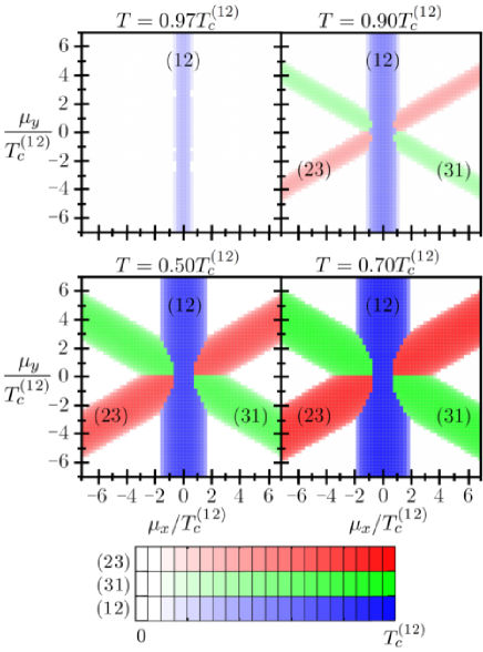
Figure 14: (Color online) Phase diagram with only approximately equal interaction strengths. The rate of the critical temperatures in the respective channels are $T_{c}^{(23)}/T_{c}^{(12)}=T_{c}^{(31)}/T_{c}^{(12)}=0.95$. The SF phase in the channel of strongest interaction repels the other two phases from the central region of the phase diagram. Parameters at the $\mu_{x}=\mu_{y}=0$ point: $(\lambda_{12},\lambda_{23},\lambda_{31})\rho_{F}=(0.1057,0.1046,0.1046),T_{c}^{(12)}W=0.01,\gamma W=0,\xi_{F}=0$.

So far we assumed a perfectly $SU(3)$ symmetrical interaction in our calculations. The phase diagram is, however, somewhat modified if the the scattering lengths are only approximately equal.UnequalInteractionStrengths ; Catelani2008 In Fig. 14 we present a phase diagram for the case where we have set the ratio of critical temperatures in the different channels to be $T_{c}^{(23)}/T_{c}^{(12)}=T_{c}^{(31)}/T_{c}^{(12)}=0.95$. For $T_{c}^{(ij)}/W\sim 0.01$ this would correspond to a $\sim 1\%$ asymmetry of the scattering lengths. At temperatures $T_{c}^{(12)}>T>T_{c}^{(23)}=T_{c}^{(31)}$ the SF phase is formed only in the $(12)$ channel. The star-like shape of the phase diagram is preserved at lower temperatures, however, the interaction asymmetry destroys the sixfold symmetry of the central region of the phase diagram, including the $O(6)$ critical point: the phase $(12)$ dominates this central region and expels the other two SF phases. Thus the shape of this region depends rather sensitively on the interaction asymmetry, and fine tuning of the scattering lengths (by using RF and MW fields,Experimental_Make_sc_lengths_equal e.g.) may be needed to realize an $SU(3)$ symmetric superfluid.

VII Conclusions

In this paper, we studied the phase diagram and the interplay of fermionic and superfluid order parameters in a three component fermionic mixture. We mostly focused on the case of $SU(3)$ symmetrical interactions, and studied the weak coupling regime, where the critical temperature is much smaller than the Fermi energy of the atoms, $T_{c}<E_{F}$. We combined two complementary mean field methods (Gaussian variational method, and equation of motion techniques) to study how a chemical potential imbalance polarizes the atomic cloud and modifies/destroys superfluid order. Though the phase diagram of the three component system is naturally much richer than that of the two component mixture,Sarma there are some similarities: large chemical potential imbalances ($|\mu_{i}-\mu_{j}|\gg T_{c}$ for all $i\neq j$), for example, destroy superfluid (SF) order, similar to two component mixtures. The corresponding SF-normal transition is of second order at higher temperatures, while it becomes of first order below the Sarma temperature.

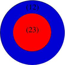
Figure 15: (Color online) Possible trap configurations for total atom numbers $N_{3}>N_{2}>N_{1}$.

The superfluid phase is, on the other hand, much richer than in the two component case. SF order can form in channels $(12)$, $(23)$, and $(31)$, and the chemical potential driven transitions between these superfluid phases are of first order. In a real experiment, where fermion numbers are approximately conserved for each component, such first order transitions would appear as segregation of different SF phases, and domain formation.Rapp Experimentally, these domains would probably appear as a shell structure, sketched in Fig. 15. For $N_{3}>N_{2}>N_{1}$, e.g., one expects that in the center of the trap a $(32)$ superfluid forms, however, approaching the external region of the trap $T_{c}$ decreases, and the $(31)$ superfluid state becomes more stable.

As a rule of thumb, SF order tends to form in the channel of the smallest chemical potential difference. This simple rule determines the overall structure of the phase diagram (see Fig 7). However, unlike the two component case, for three component mixtures a non-trivial coupling between magnetic and SF order is also allowed.Demler ; Rapp This interesting coupling — the strength of which is regulated by particle-hole symmetry breaking, $\gamma\sim\varrho^{\prime}(E_{F})/\varrho(E_{F})\sim 1/E_{F}$ — leads to a peculiar triangular structure in the central region of the phase diagram, $\mu_{i}\approx\mu$, in agreement with the predictions of Ref. Demler, (though with opposite orientation, see Fig 7). However, the relative size of this central region is apparently proportional to $\sim\sqrt{\gamma T_{c}}$; therefore, for weak and intermediate couplings, the triangular structure appears only in the close vicinity of the $SU(3)$ symmetrical point, $\mu_{i}\equiv\mu$. For very strong attractive interactions, $T_{c}\approx E_{F}\sim W$, on the other hand, the central (triangular) region must get more extended, and may become observable.

We also constructed the Ginzburg-Landau functionals describing the three component mixture, and determined the temperature and asymmetry ($\gamma$) dependence of the various coefficients. We have shown that, to capture the termination of the central triangular region, one needs to go beyond the expansion of Ref. Demler, , and higher order terms need be incorporated in the functionals.

As discussed in Sec. V, fluctuations modify somewhat the mean-field picture. The temperature-driven phase transition for generic (unequal) chemical potential values is typically described by the XY model and its critical exponents. However, for certain special chemical potentials, the competition between various superfluid orders may lead to interesting critical behavior. For $\mu_{i}\equiv\mu$ and an $SU(3)$ symmetrical interaction, e.g., the normal-SF transition belongs to the $O(6)$ universality class, and is characterized by the corresponding exponents. Along the critical lines separating the three phases, $(12)$, $(23)$, and $(31)$, on the other hand, an interesting $O(2,2)$ critical behavior may emerge (see our discussion in Sec. V). The shape of the phase diagram in the vicinity of these special lines is then determined by the corresponding universal cross-over exponents. We emphasize that – while it is very difficult to observe it in the weak coupling regime – a non-trivial critical behavior could be observable in the strong coupling regime, often reached in cold atom experiments.

Finally, we studied the fragility of the $SU(3)$ physics, i.e., the sensitivity of these results and the phase diagram to the symmetry of interaction. We have shown that already a small difference in the scattering lengths can substantially distort the $SU(3)$ phase diagram, and the SF phase of the channel with the strongest interaction may suppress and mask the $SU(3)$ symmetrical ($O(6)$) critical regime. These results agree with those obtained in Ref. Catelani2008, . Here, however, in contrast to Ref. Catelani2008, , we focused on the consequences of SU(3) symmetry (rather than on the consequences of its violation), and the effects of the coupling between ferromagnetic and superfluid order parameters, neglected in Ref. Catelani2008, . In addition, we also discussed the role of fluctuations and the structure of the emerging critical states and multicritical lines. Our results as well as those of Ref. Catelani2008, indicate that in experimental realizations, to observe the $SU(3)$ physics, one should use systems with almost perfectly symmetrical interactions, similar to YbYbSymmetric , or one should use some tricks to make all scattering lengths equal as much as possible.Experimental_Make_sc_lengths_equal Moreover, one should possibly stay in the strong coupling regime, $T_{c}\sim W$, where the impact of a small asymmetry in the interaction is not exponentially large.

VIII Acknowledgment

We would like to thank Eugene Demler, Gil Refael, and Walter Hofstetter for enlightening discussions. This research has been supported by the Hungarian research funds OTKA and NKTH under Grant Nos. K73361 and CNK80991. G.Z. acknowledges support from the Humboldt Foundation and the DFG.

Appendix A Exact Ward identities

In this Appendix, by making use of the global $SU(3)$ invariance of the functional measure, we derive exact Ward identities that give constraints on the possible values of the order parameters and densities, Eqs. (6-9).

Consider the partition function $\mathcal{Z}$, defined in Eq. (12). For the current calculation we rewrite the action Eqs. (13,14) in the form

$$S_{0}(\hat{\mu}) =\sum_{\alpha\beta}\int\mathrm{d}x\,\overline{\psi}_{\alpha}\left((\partial_{\tau}+\mathcal{H}_{0})\delta_{\alpha\beta}-\hat{\mu}_{\alpha\beta}\right)\psi_{\beta},$$ (51)

$$S_{\mathrm{int}}(\Gamma) =-\sum_{\alpha\beta\gamma\delta}\Gamma_{\alpha\beta\gamma\delta}\int\mathrm{d}x\,\overline{\psi}_{\alpha}\overline{\psi}_{\beta}\psi_{\gamma}\psi_{\delta}\;.$$ (52)

by introducing $\hat{\mu}_{\alpha\beta}=\mu_{\alpha}\,\delta_{\alpha\beta}$ and $\Gamma_{\alpha\beta\gamma\delta}=\frac{1}{2}\lambda_{\alpha\beta}\left(\delta_{\alpha\delta}\delta_{\beta\gamma}-\delta_{\alpha\gamma}\delta_{\beta\delta}\right)$. An $SU(3)$ transformation of the fields $\psi_{\alpha}(x)\rightarrow\sum_{\beta}U_{\alpha\beta}\psi_{\beta}(x)$ translates to the transformation of $\hat{\mu}$ and $\Gamma$ in the functional integral. Expressing $\mathbf{U}=\exp(i\sum_{a=1}^{8}\eta^{a}\mathbf{T}^{a})$ with the Gell-Mann matrices $\mathbf{T}^{a}$, we find

$$\left.\frac{\partial}{\partial\eta^{a}}\hat{\mu}_{\alpha\beta}(\eta)\right|_{\eta^{a}=0} =i\sum_{\gamma}\left(\hat{\mu}_{\alpha\gamma}T^{a}_{\gamma\beta}-T^{a}_{\alpha\gamma}\hat{\mu}_{\gamma\beta}\right),$$ (53)

$$\left.\frac{\partial}{\partial\eta^{a}}\Gamma_{\alpha\beta\gamma\delta}(\eta)\right|_{\eta^{a}=0} =2i\left(\lambda_{\alpha\beta}-\lambda_{\gamma\delta}\right)\delta_{\alpha\delta}\,T^{a}_{\beta\gamma}\;.$$ (54)

The invariance of the functional integral with respect to global $SU(3)$ transformations, $\left.\frac{\partial\mathcal{Z}}{\partial\eta^{a}}\right|_{\eta_{a}=0}=0$, leads to the Ward identity

$$\left(\mu_{\alpha}-\mu_{\beta}\right)\frac{\partial\mathrm{ln}\mathcal{Z}}{\partial\hat{\mu}_{\alpha\beta}}=2\sum_{\gamma}\left(\lambda_{\beta\gamma}-\lambda_{\alpha\gamma}\right)\frac{\partial\mathrm{ln}\mathcal{Z}}{\partial\Gamma_{\gamma\alpha\beta\gamma}},$$ (55)

for any $\alpha$ and $\beta$, from which Eq. (32) follows.

Appendix B Ward identities in the Gaussian approximation

Here, we derive approximate Ward identities, similar to those in Appendix A, that hold in the Gaussian approximation. As explained in Appendix C, we can assume that the inverse propagator in the definition of the partition function $\mathcal{Z_{D}}$, Eq. (18), is local,

$$\mathcal{Z}_{\mathcal{D}}=\int\mathfrak{D}\mathbf{\overline{\psi}}\,\mathfrak{D}\mathbf{\psi}\,e^{\frac{1}{2}\int\mathrm{d}1\,\overline{\phi}(1)\mathbf{D}^{-1}(1)\phi(1)},$$ (56)

where $\mathbf{D}^{-1}$ is defined in Eq. (23).

An $SU(3)$ transformation of the fields $\psi_{\alpha}(x)\rightarrow\sum_{\beta}U_{\alpha\beta}\psi_{\beta}(x)$ translates to the transformation of order parameters,

$$\mathbf{\Lambda} \mapsto\mathbf{U}\mathbf{\Lambda}\mathbf{U}^{+},$$ (57)

$$\mathbf{\Delta} \mapsto\mathbf{U}\mathbf{\Delta}\mathbf{U}^{\mathrm{T}},$$ (58)

see Eqs. (29,30). Using the invariance of the partition function with respect to these global $SU(3)$ transformations, we get the following constraints on the densities,

$$\mathrm{Tr}\left(\begin{pmatrix}\mathbf{\Gamma}_{\mathbf{\Lambda}}^{a}&\mathbf{\Gamma}_{\mathbf{\Delta}}^{a}\\ -\mathbf{\Gamma}_{\mathbf{\Delta}}^{a+}&\mathbf{\Gamma}_{\mathbf{\Lambda}}^{a*}\end{pmatrix}\begin{pmatrix}-\mathbf{n}^{*}&\mathbf{d}\\ \mathbf{d}^{+}&\mathbf{n}\end{pmatrix}\right)=0\;,$$ (59)

with $\mathbf{\Gamma}_{\mathbf{\Lambda}}^{a}=\left[\mathbf{\Lambda},\mathbf{T}^{a}\right]$ and $\mathbf{\Gamma}_{\mathbf{\Delta}}^{a}=2\left(\mathbf{T}^{a}\mathbf{\Delta}+\mathbf{\Delta}\mathbf{T}^{a*}\right)$.footnote7 Here the matrices $\mathbf{T}^{a}$, $a=1,\dots,8$, are the Gell-Mann matrices.

In case of $SU(3)$ symmetric interactions, at the solutions of the EOM equations, Eqs. (6,7,10), this equation simplifies to the same form as the exact Ward identity, Eq. (32),

$$\left(\mu_{\alpha}-\mu_{\beta}\right)n_{\alpha\beta}=0\;.$$ (60)

Therefore, when neither two of the chemical potentials are equal, the matrix of densities $\mathbf{n}$ and that of renormalized chemical potentials $\mathbf{\Lambda}$ are both diagonal (see Eq. (7)).

Appendix C Saddle point equation in the Gaussian approximation

In this Appendix, starting from the saddle point equation, Eq. (21), we derive the saddle point form of the propagator $\mathcal{D}$ in the Gaussian approximation, Eqs. (22,23). We will use the notations of Section II.2.

First, we fix the arbitrariness in the form of $\mathcal{D}^{-1}$ in the definition of $S_{\mathcal{D}}$, Eq. (17). We split $\mathcal{D}^{-1}$ into $3\times 3$ matrices

$$\mathcal{D}^{-1}(1,2)=\begin{pmatrix}\mathbf{\Gamma}_{A}(x_{1},x_{2})&\mathbf{\Gamma}_{B}(x_{1},x_{2})\\ \mathbf{\Gamma}_{C}(x_{1},x_{2})&\mathbf{\Gamma}_{D}(x_{1},x_{2})\end{pmatrix}.$$ (61)

It is easy to see, that because of the anticommutation of the fields $\overline{\psi}_{\alpha}$ and $\psi_{\alpha}$, modifications of $\mathcal{D}^{-1}$ that leave $\mathbf{\Gamma}_{A}(x_{1},x_{2})-\mathbf{\Gamma}_{D}^{T}(x_{2},x_{1})$, $\mathbf{\Gamma}_{B}(x_{1},x_{2})-\mathbf{\Gamma}_{B}^{T}(x_{2},x_{1})$ and $\mathbf{\Gamma}_{C}(x_{1},x_{2})-\mathbf{\Gamma}_{C}^{T}(x_{2},x_{1})$ invariant, will not change $S_{\mathcal{D}}$. Therefore we may assume that $\mathcal{D}^{-1}$ has the symplectic symmetry

$$\begin{pmatrix}\mathbf{0}&\mathbf{1}\\ \mathbf{1}&\mathbf{0}\end{pmatrix}\,\mathcal{D}^{-1}(x_{1},x_{2})\,\begin{pmatrix}\mathbf{0}&\mathbf{1}\\ \mathbf{1}&\mathbf{0}\end{pmatrix}=-\left(\mathcal{D}^{-1}\right)^{\mathrm{T}}(x_{2},x_{1}).$$ (62)

The saddle point equation, Eq. (21), gives very strong constraints on the form of $\mathcal{D}$. In particular, it is equivalent to the EOM self-consistency equation of Section II.1. To see this, we use the definition Eq. (16) to rewrite Eq. (21) in the form

$$\frac{1}{\mathcal{Z}_{\mathcal{D}}}\,\frac{\delta\mathcal{Z}_{\mathcal{D}}}{\delta\mathcal{D}(1,2)}=\frac{\delta\langle S-S_{\mathcal{D}}\rangle_{\mathcal{D}}}{\delta\mathcal{D}(1,2)}.$$ (63)

The calculation of the left hand side of this equation is straightforward. Using only the definition of $\mathcal{Z_{D}}$ (see Eq. (18)), and Eq. (20), we get

$$\frac{1}{\mathcal{Z}_{\mathcal{D}}}\,\frac{\delta\mathcal{Z}_{\mathcal{D}}}{\delta\mathcal{D}(1,2)}=-\frac{1}{2}\mathcal{D}^{-1}(2,1).$$ (64)

To evaluate the right hand side of Eq. (63), omitting a constant term, we can write

$$\langle S-S_{\mathcal{D}}\rangle_{\mathcal{D}}=-\frac{1}{2}\int\mathrm{d}1\,\mathrm{d}2\,\mathcal{D}_{0}^{-1}(1,2)\mathcal{D}(2,1)+\langle S_{\mathrm{int}}\rangle_{\mathcal{D}}.$$ (65)

Then, it is easy to see that, the saddle point equation is equivalent to

$$\mathcal{D}^{-1}(1,2)=\mathcal{D}_{0}^{-1}(1,2)-2\,\frac{\delta\langle S_{\mathrm{int}}\rangle_{\mathcal{D}}}{\delta\mathcal{D}(2,1)}.$$ (66)

Expanding $\langle S_{\mathrm{int}}\rangle_{\mathcal{D}}$ using Wick’s theorem gives a product of equal time propagators, whose variation according to the propagator matrix $\mathcal{D}$ can be straightforwardly calculated. We get the desired formulas, Eqs. (22,23), with the order parameters $\mathbf{\Lambda}$ and $\mathbf{\Delta}$ satisfying the EOM self-consistency equations, Eqs. (6,7), and (10). This means, that the EOM method is consistent with the Gaussian variational approach.

Appendix D Calculation of the Gaussian approximation to the free energy

In the following we calculate the Gaussian approximation of the free energy, Eq.(25). We first introduce the Fourier components $\psi_{\alpha}(\mathbf{r})=\frac{1}{\sqrt{\Omega}}\sum_{\mathbf{k}}e^{i\mathbf{kr}}a_{\alpha\mathbf{k}}$, obeying the anti-commutation relations $\{a^{\dagger}_{\mathbf{k}\alpha},a_{\mathbf{k}^{\prime}\beta}\}=\delta_{\alpha\beta}\,\delta_{\mathbf{k}\mathbf{k}^{\prime}}$, where $\Omega$ denotes the volume. With these, the Hamiltonian, Eq. (24), takes on the form

$$H_{\mathcal{D}}=\frac{1}{2}\sum_{\mathbf{k}}\left\{\left(\mathbf{a}^{\dagger}_{\mathbf{k}},\mathbf{a}_{-\mathbf{k}}\right)\mathbf{B}(\xi_{\mathbf{k}})\begin{pmatrix}\mathbf{a}_{\mathbf{k}}\\ \mathbf{a}^{\dagger}_{-\mathbf{k}}\end{pmatrix}+\mathrm{Tr}\left(\xi_{\mathbf{k}}-\mathbf{\Lambda}\right)\right\},$$ (67)

with $\mathbf{B}(\xi)$ defined in Eq. (5), and the last term originating from normal ordering.

From the above form, the calculation of $\mathcal{Z}_{\mathcal{D}}=\mathrm{Tr}e^{-\beta H_{\mathcal{D}}}$ is straightforward, though some care is needed to avoid double counting in momentum space. Note that, because of the symplectic symmetry, Eq. (11), and Hermiticity of the matrix $\mathbf{B}(\xi)$, its eigenvalues are real and come in pairs. To each eigenvalue $\eta(\xi)$ there is another eigenvalue $-\eta\left(\xi\right)$. Using this property, $\log\mathcal{Z}_{\mathcal{D}}$ simplifies to

$$\log\mathcal{Z}_{\mathcal{D}}= \frac{1}{2}\sum_{\mathbf{k}}\mathrm{Tr}\log\left(2\cosh\left(\frac{\beta}{2}\mathbf{B}\left(\xi_{\mathbf{k}}\right)\right)\right)$$ (68)

$$- \frac{\beta}{2}\sum_{\mathbf{k}}\mathrm{Tr}\left(\xi_{\mathbf{k}}-\mathbf{\Lambda}\right).$$

The calculation of $\langle H-H_{\mathcal{D}}\rangle_{\mathcal{D}}$ is also straightforward using Wick’s theorem. One finds

$$\frac{1}{\Omega}\langle H-H_{\mathcal{D}}\rangle_{\mathcal{D}}= \sum_{\alpha\beta}\lambda_{\alpha\beta}(\left|n_{\alpha\beta}\right|^{2}-n_{\alpha\alpha}n_{\beta\beta}-\left|d_{\alpha\beta}\right|^{2})$$

$$+ \sum_{\alpha\beta}\left(\Lambda_{\alpha\beta}-\mu_{\alpha}\delta_{\alpha\beta}\right)n_{\alpha\beta}$$ (69)

$$+ \sum_{\alpha\beta}\Delta_{\alpha\beta}d^{*}_{\alpha\beta}+\Delta^{*}_{\alpha\beta}d_{\alpha\beta}.$$

Thus, using Eqs. (68,69), we get the result Eq. (28) for the Gaussian approximation of the free energy density .

In order to evaluate Eq. (69), the densities and anomalous densities, $\mathbf{n}$ and $\mathbf{d}$, also have to be determined. These can be easily calculated from the variations of (68) with respect to $\mathbf{\Lambda}$ and $\mathbf{\Delta}$, leading to the same equation, Eq. (10), as the EOM self-consistency equations.

Appendix E Particle-hole transformation

Particle-hole symmetry introduces a $\mathbb{Z}_{2}$ symmetry of the mean-field phase diagram, when the band is half-filled, the DOS is particle-hole symmetric ($\rho(\xi)=\rho(-\xi)$), and the interaction has $SU(3)$ symmetry ($\lambda_{\alpha\neq\beta}=\lambda$). This symmetry together with the permutation symmetry of the fermion species makes the phase diagram six-fold symmetric, see Fig. 1.

In this Appendix we calculate the effect of the particle-hole transformation

$$\Psi_{\alpha}(x)\longleftrightarrow\Psi^{\dagger}_{\alpha}(x)$$ (70)

on the order parameters $\mathbf{\Lambda}$ and $\mathbf{\Delta}$. This transformation leaves the interaction invariant, whereas it modifies the bare chemical potentials and the single particle energies as

$$\mathcal{H}_{0} \rightarrow -\mathcal{H}_{0},$$ (71)

$$\mu_{\alpha} \rightarrow -\mu_{\alpha}-4\lambda\,n_{\mathrm{max}},$$ (72)

where $n_{\mathrm{max}}=\int_{-W}^{W}\mathrm{d}\xi\,\rho(\xi)$ is the density of the completely filled band. The bare chemical potentials remain unchanged on the mean-field level at

$$\mu_{\mathrm{half}}=-2\lambda\,n_{\mathrm{max}},$$ (73)

which is precisely the condition for the band being half-filled (see Eq. (7)).

In order to investigate the inversion symmetry of the phase diagram, consider two Hamiltonians with opposite differences in bare chemical potentials from half-filling,

$$H^{(1)} \equiv H(\mathcal{H}_{0},\mu_{\mathrm{half}}+\delta\mu_{\alpha},\lambda,\Psi^{\dagger}_{\alpha},\Psi_{\alpha}),$$ (74)

$$H^{(2)} \equiv H(\mathcal{H}_{0},\mu_{\mathrm{half}}-\delta\mu_{\alpha},\lambda,\Psi^{\dagger}_{\alpha},\Psi_{\alpha}),$$ (75)

as defined in Eq. (I). A particle-hole transformation of $H^{(2)}$ leads to the equation

$$H^{(2)}=H(-\mathcal{H}_{0},\mu_{\mathrm{half}}+\delta\mu_{\alpha},\lambda,\widetilde{\Psi}^{\dagger}_{\alpha},\widetilde{\Psi}_{\alpha})\equiv H^{(3)},$$ (76)

where $\widetilde{\Psi}_{\alpha}=\Psi^{\dagger}_{\alpha}$. Accordingly, the densities in the original and the particle-hole transformed system can be connected as

$$n_{\alpha\beta}^{(3)} \equiv \langle\widetilde{\Psi}^{\dagger}_{\alpha}(x)\widetilde{\Psi}_{\beta}(x)\rangle_{(3)}=-n_{\alpha\beta}^{(2)*}+n_{\mathrm{max}},$$ (77)

$$d_{\alpha\beta}^{(3)} \equiv \langle\widetilde{\Psi}_{\alpha}(x)\widetilde{\Psi}_{\beta}(x)\rangle_{(3)}=-d_{\alpha\beta}^{(2)*}.$$ (78)

Then, it is also straightforward to show from the definitions Eqs. (6,7), that the relation between the order parameters are

$$\mathbf{\Lambda}^{(2)}=-\mathbf{\Lambda}^{(3)*},\hskip 12.0pt\mathbf{\Delta}^{(2)}=-\mathbf{\Delta}^{(3)*}.$$ (79)

Looking at their definitions, we see that the only difference between $H^{(2)}$ and $H^{(3)}$ is in the sign of $\mathcal{H}_{0}$. However, if the DOS is electron-hole symmetric,

$$\rho(\xi)=\rho(-\xi),$$ (80)

then all of the EOM self-consistency equations Eqs. (6,7,10), and the mean-field free energy Eqs. (10,28) are identical in the two systems. Therefore, the set of the possible mean-field configurations have to be the same ($\mathbf{\Lambda}^{(1)}=\mathbf{\Lambda}^{(3)}$, $\mathbf{\Delta}^{(1)}=\mathbf{\Delta}^{(3)}$). Putting this, and Eq. (79) together, we obtain the desired equations

$$\mathbf{\Lambda}(\mu_{\mathrm{half}}+\delta\mu_{\alpha}) = -\mathbf{\Lambda}^{*}(\mu_{\mathrm{half}}-\delta\mu_{\alpha}),$$ (81)

$$\mathbf{\Delta}(\mu_{\mathrm{half}}+\delta\mu_{\alpha}) = -\mathbf{\Delta}^{*}(\mu_{\mathrm{half}}-\delta\mu_{\alpha}),$$ (82)

connecting order parameters at opposite $\delta\mu_{\alpha}$ values, with the other parameters of the system unchanged.

We remark, that in the special case when $\delta\mu_{1}+\delta\mu_{2}+\delta\mu_{3}=0$, the particle-hole symmetry connects the points of the same $(\mu_{x},\mu_{y})$ plane, and the mean-field phase diagram has an inversion symmetry. Away from this plane the inversion symmetry is only approximate, due to logarithmic corrections to the values of the order parameters, coming from the asymmetric cut-off.

References

- (1) I. Bloch, J. Dalibard, W. Zwerger, Rev. Mod. Phys. 80, 885 (2008).
- (2) M. P. A. Fisher, P. B. Weichman, G. Grinstein, and D. S. Fisher, Phys. Rev. B 40, 546 (1989); D. Jaksch, C. Bruder, J. I. Cirac, C. W. Gardiner, and P. Zoller, Phys. Rev. Lett. 81, 3108 (1998); M. Greiner, M. O. Mandel, T. Esslinger, T. Hänsch, and I. Bloch, Nature 415, 39 (2002).
- (3) J. K. Chin, D. E. Miller, Y. Liu, C. Stan, W. Setiawan, C. Sanner, K. Xu, and W. Ketterle, Nature 443, 961 (2006).
- (4) C. Chin, M. Bartenstein, A. Altmeyer, S. Riedl, S. Jochim, J. Hecker Denschlag, and R. Grimm, Science 305, 1128 (2004); M. W. Zwierlein, C. A. Stan, C. H. Schunck, S. M. F. Raupach, A. J. Kerman, and W. Ketterle, Phys. Rev. Lett. 92, 120403 (2004); C. A. Regal, M. Greiner, and D. S. Jin, Phys. Rev. Lett. 92, 040403 (2004); J. Kinast, S. L. Hemmer, M. E. Gehm, A. Turlapov, and J. E. Thomas, Phys. Rev. Lett. 92, 150402 (2004).
- (5) M. W. Zwierlein, C. H. Schunck, A. Schirotzek, and W. Ketterle, Nature 442, 54 (2006).
- (6) G. B. Partridge, W. Li, R. I. Kamar, Y. Liao, and R. G. Hulet, Science 311, 503 (2006).
- (7) M. W. Zwierlein, A. Schirotzek, C. H. Schunck, and W. Ketterle, Science 311, 492 (2006).
- (8) Y. Shin, C. H. Schunck, A. Schirotzek, and W. Ketterle, Nature 451, 689 (2008).
- (9) M. W. Zwierlein, J. R. Abo-Shaeer, A. Schirotzek, C. H. Schunck, and W. Ketterle, Nature 435, 1047 (2005).
- (10) M. H. Anderson, J. R. Ensher, M. R. Matthews, C. E. Wieman, and E. A. Cornell, Science 269, 198 (1995); C. C. Bradley, C. A. Sackett, J. J. Tollett, and R. G. Hulet, Phy. Rev. Lett. 75, 1687 (1995); K. B. Davis, M.-O. Mewes, M. R. Andrews, N. J. van Druten, D. S. Durfee, D. M. Kurn, and W. Ketterle, Phys. Rev. Lett. 75, 3969 (1995); M. R. Andrews, C. G. Townsend, H.-J. Miesner, D. S. Durfee, D. M. Kurn, and W. Ketterle, Science 275, 637 (1997).
- (11) K. E. Strecker, G. B. Partridge, A. G. Truscott, and R. G. Hulet, Nature 417, 150 (2002); L. Khaykovich, F. Schreck, G. Ferrari, T. Bourdel, J. Cubizolles, L. D. Carr, Y. Castin, and C. Salomon, Science 296, 1290 (2002).
- (12) L. S. Leslie, A. Hansen, K. C. Wright, B. M. Deutsch, and N. P. Bigelow, Phys. Rev. Lett. 103, 250401 (2009); J. Ruostekoski and J. R. Anglin, Phys. Rev. Lett. 86, 3934 (2001); C. M. Savage and J. Ruostekoski, Phys. Rev. Lett. 91, 010403 (2003); V. Pietilä and M. Möttönen, Phys. Rev. Lett. 103, 030401 (2009).
- (13) E. Babaev, L. D. Faddeev, and A. J. Niemi, Phys. Rev. B 65, 100512(R) (2002).
- (14) Y.-J. Lin, R. L. Compton, K. Jiménez-García, J. V. Porto, and I. B. Spielman, Nature 452, 628 (2009); J. Dalibard, F. Gerbier, G. Juzeliunas, P. Ohberg, Rev. Mod. Phys. 83, 1523 (2011); N. Cooper, Phys. Rev. Lett. 106, 175301 (2011).
- (15) C. Honerkamp, and W. Hofstetter, Phys. Rev. Lett. 92, 170403 (2004).
- (16) Á. Rapp, G. Zaránd, C. Honerkamp, and W. Hofstetter, Phys. Rev. Lett. 98, 160405 (2007); Á. Rapp, W. Hofstetter, and G. Zaránd, Phys. Rev. B 77, 144520 (2008).
- (17) J. H. Huckans, J. R. Williams, E. L. Hazlett, R. W. Stites, and K. M. O’Hara, Phys. Rev. Lett. 102, 165302 (2009); J. R. Williams, E. L. Hazlett, J. H. Huckans, R. W. Stites, Y. Zhang, and K. M. O’Hara, Phys. Rev. Lett. 103, 130404 (2009).
- (18) A. Kantian, M. Dalmonte, S. Diehl, W. Hofstetter, P. Zoller, and A. J. Daley, Phys. Rev. Lett. 103, 240401 (2009).
- (19) T. Kraemer, M. Mark, P. Waldburger, J. G. Danzl, C. Chin, B. Engeser, A. D. Lange, K. Pilch, A. Jaakkola, H.-C. Nägerl, and R. Grimm, Nature 440, 315 (2006).
- (20) T. B. Ottenstein, T. Lompe, M. Kohnen, A. N. Wenz, and S. Jochim, Phys. Rev. Lett. 101, 203202 (2008).
- (21) A. V. Gorshkov, M. Hermele, V. Gurarie, C. Xu, P. S. Julienne, J. Ye, P. Zoller, E. Demler, M. D. Lukin, and A. M. Rey, Nature Phys. 6, 289 (2010).
- (22) C. Wu, J. Hu, and S. Zhang, Phys. Rev. Lett. 91, 186402 (2003).
- (23) D. S. Sarma, J. Phys. Chem. Solids 24, 1029 (1963).
- (24) R. W. Cherng, G. Refael, and E. Demler, Phys. Rev. Lett. 99, 130406 (2007).
- (25) I. Titvinidze, A. Privitera, S.-Y. Chang, S. Diehl, M. A. Baranov, A. Daley, and W. Hofstetter, New. J. Phys. 13, 035013 (2011).
- (26) Note that our convention for the interaction strength differs from the usual convention by a factor of 1/2. This difference also affects the definitions of the order parameters later, see Eqs. (6,7).
- (27) M. Bartenstein, A. Altmeyer, S. Riedl, R. Geursen, S. Jochim, C. Chin, J. Hecker Denschlag, R. Grimm, A. Simoni, E. Tiesinga, C. J. Williams, and P. S. Julienne, Phys. Rev. Lett. 94, 103201 (2005).
- (28) K. M. O’Hara, New. J. Phys. 13, 065011 (2011).
- (29) Notice that the chemical potentials in Eq. (I) are chosen to be zero in the middle of the single particle energy band, .
- (30) C. Honerkamp, W. Hofstetter, Phys. Rev. B 70, 094521 (2004).
- (31) Part of the interaction is decomposed in the superfluid channel, while the other part in the ferromagnetic channel, and thus part of the interaction energy is apparently dropped.
- (32) P. Fulde, R. A. Ferrell, Phys. Rev. 135, A550 (1964).
- (33) A. I. Larkin, Yu. N. Ovchinnikov, Zh. Eksp. Teor. Fiz. 47, 1136 (1964); A. I. Larkin, Yu. N. Ovchinnikov, Sov. Phys. JETP 20, 762 (1965).
- (34) W. V. Liu and F. Wilczek, Phys. Rev. Lett. 90, 047002 (2003); M. M. Forbes, E. Gubankova, W. V. Liu, and F. Wilczek, Phys. Rev. Lett. 94, 017001 (2005).
- (35) Of course, particle-hole symmetry can be broken in many other ways, too (by introducing an asymmetrical cut-off, , e.g.), but the non-vanishing slope of the DOS seems to have the largest impact.
- (36) We remark that our definition of the SF order parameter differs from the usual convention by a factor of 1/2. This comes from the factor 1/2 difference in our convention for the interaction parameter in Eq. (I).
- (37) R. P. Feynman, Statistical Mechanics: A Set of Lectures, Perseus Books Group, 2nd edition (1998).
- (38) We verified that, indeed, this normal ordering provides the correct densities at the free energy minima.
- (39) A. M. Clogston, Phys. Rev. Lett. 9, 266 (1962).
- (40) In case of a linear DOS, is slightly greater than for positive ’s, while it is slightly smaller than for .
- (41) Since the simultaneous shift of all the chemical potential components shall have no impact apart from changing the value of the Ginzburg-Landau coefficients, we restrict ourselves to .
- (42) Notice that the term is proportional to , and does not appear in the expansion.
- (43) L. He, M. Jin, and P. Zhuang, Phys. Rev. A 74, 033604 (2006).
- (44) Z. Hadzibabic, P. Krüger, M. Cheneau, B. Battelier, and J. Dalibard, Nature 441, 1118 (2006).
- (45) H. Kleinert, J. Neu, V. Schulte-Frohlinde, K. G. Chetyrkin, and S. A. Larin, Phys. Lett. B 272, 39 (1991).
- (46) S. A. Antonenko and A. I. Sokolov, Phys. Rev. E 51, 1894 (1995).
- (47) P. Butera, and M. Comi, Phys. Rev. B 56, 8212 (1997).
- (48) D. Loison, Physica A 271, 157 (1999).
- (49) M. Campostrini, M. Hasenbusch, A. Pelissetto, P. Rossi, and E. Vicari, Phys. Rev. B 63, 214503 (2001); R. Guida, J. Zinn-Justin, J. Phys. A: Math. Gen. 31, 8103 (1998).
- (50) J. M. Kosterlitz and D. J. Thouless, J. Phys. C: Solid State Phys. 6, 1181 (1973).
- (51) E. Brezin, J. C. Le Guillou, and J. Zinn-Justin, Phys. Rev. B 10, 892 (1974); D. Mukamel and S. Krinsky, Phys. Rev. B 13, 5065 (1976); D. Mukamel and S. Krinsky, Phys. Rev. B 13, 5078 (1976); E. Domany, D. Mukamel, and E. Fisher, Phys. Rev. B 15, 5432 (1977); J. C. Toledano, L. Michel, P. Toledano, E. Brezin, Phys. Rev. B 31, 7171 (1985); M. Dudka, Y. Holovatch, T. Yavors’kii, J. Phys. A: Math. Gen. 37, 10727-10734 (2004).
- (52) J. M. Kosterlitz, D. R. Nelson, and M. E. Fisher, Phys. Rev. B 13, 412 (1976).
- (53) A. Aharony in Phase Transitions and Critical Phenomna, Volume 6, edited by C. Domb and M. S. Green (Academic Press, 1977).
- (54) D. Mukamel, Phys. Rev. Lett. 34, 481 (1975).
- (55) P. Calabrese, A. Pelissetto, and E. Vicari, Phys. Rev. B 67, 054505 (2003).
- (56) E. Vicari and J. Zinn-Justin, New J. Phys. 8, 321 (2006).
- (57) A. Aharony and S. Fishman, Phys. Rev. Lett. 37, 1587 (1976); R. A. Cowley, A. D. Bruce, J. Phys. C: Solid State Phys. 11, 3577 (1978); A. Aharony, Phys. Rev. Lett. 88, 059703 (2002).
- (58) J. Cardy, Scaling and Renormalization in Statistical Physics, Cambridge Lecture Notes in Physics (1996).
- (59) In the absence of particle-hole symmetry, one may need to rescale the fields and to have the same coefficient in the kinetic part.
- (60) M. Kanász-Nagy, unpublished.
- (61) T. Paananen, J.-P. Martikainen, and P. Törmä, Phys. Rev. A 73, 053606 (2006).
- (62) G. Catelani and E. A. Yuzbashyan, Phys. Rev. A 78, 033615 (2008).
- (63) M. Kitagawa, K. Enomoto, K. Kasa, Y. Takahashi, R. Ciurylo, P. Naidon, and P. S. Julienne, Phys. Rev. A 77, 012719 (2008).
- (64) We note, that Eq. (59) holds only at the solutions of the EOM self-consistency equations.
- (65) We assume that for each counter-propagating momenta the single particle energies are the same, . (This follows naturally from the inversion symmetry of the system.) This property makes the calculations in the Cooper channel simple, since in each vertex both of the energies of the incoming lines, and both of those of the outgoing lines are either in , or neither of them is. Therefore the energies that we integrate out can be trivially separated in the calculation of ladder diagrams.
- (66) A. J. Leggett in Modern Trends in the Theory of Condensed Matter, edited by A. Pekalski and J. Przystawa (Springer-Verlag, Berlin, 1980).
- (67) Q. Chen, J. Stajic, S. Tan, K. Levin, Phys. Rep. 412, 1 (2005).