Negative-energy $\mathcal{P}\mathcal{T}$-symmetric Hamiltonians

Abstract

The non-Hermitian $\mathcal{P}\mathcal{T}$-symmetric quantum-mechanical Hamiltonian $H=p^{2}+x^{2}(ix)^{\varepsilon}$ has real, positive, and discrete eigenvalues for all $\varepsilon\geq 0$. These eigenvalues are analytic continuations of the harmonic-oscillator eigenvalues $E_{n}=2n+1$ ($n=0,\,1,\,2,\,3,\,\ldots$) at $\varepsilon=0$. However, the harmonic oscillator also has negative eigenvalues $E_{n}=-2n-1$ ($n=0,\,1,\,2,\,3,\,\ldots$), and one may ask whether it is equally possible to continue analytically from these eigenvalues. It is shown in this paper that for appropriate $\mathcal{P}\mathcal{T}$-symmetric boundary conditions the Hamiltonian $H=p^{2}+x^{2}(ix)^{\varepsilon}$ also has real and negative discrete eigenvalues. The negative eigenvalues fall into classes labeled by the integer $N$ ($N=1,\,2,\,3,\,\ldots$). For the $N$th class of eigenvalues, $\varepsilon$ lies in the range $(4N-6)/3<\varepsilon<4N-2$. At the low and high ends of this range, the eigenvalues are all infinite. At the special intermediate value $\varepsilon=2N-2$ the eigenvalues are the negatives of those of the conventional Hermitian Hamiltonian $H=p^{2}+x^{2N}$. However, when $\varepsilon\neq 2N-2$, there are infinitely many complex eigenvalues. Thus, while the positive-spectrum sector of the Hamiltonian $H=p^{2}+x^{2}(ix)^{\varepsilon}$ has an unbroken $\mathcal{P}\mathcal{T}$ symmetry (the eigenvalues are all real), the negative-spectrum sector of $H=p^{2}+x^{2}(ix)^{\varepsilon}$ has a broken $\mathcal{P}\mathcal{T}$ symmetry (only some of the eigenvalues are real).

I Introduction

In 1993 an observation was made R1 regarding the eigenvalues of the conventional quantum-harmonic-oscillator Hamiltonian

$$H=p^{2}+\omega^{2}x^{2},$$ (1)

where $\omega$ is a real positive parameter. It was noted that while the standard eigenvalues of $H$ are real and positive

$$E_{n}=(2n+1)\omega\qquad(n=0,\,1,\,2,\,3,\,\ldots),$$ (2)

if (1) and (2) are analytically continued in the complex-$\omega$ plane from positive to negative $\omega$, the eigenvalues $E_{n}$ all become negative even though the Hamiltonian (1) appears to remain unchanged. Surprisingly, the harmonic-oscillator Hamiltonian (1), which is a sum of squares, also possesses an infinite set of negative eigenvalues.

A careful treatment of the boundary conditions on the eigenfunctions is required to explain the appearance of negative eigenvalues. The conventional boundary conditions associated with the Schrödinger eigenvalue differential equation

$$-\psi^{\prime\prime}(x)+\omega^{2}x^{2}\psi(x)=E\psi(x)$$ (3)

are that $\psi(x)\to 0$ as $x\to\pm\infty$ on the real axis. These boundary conditions hold not just on the real axis but in Stokes wedges centered about the positive-real and negative-real axes in the complex-$x$ plane R2 . Specifically, the eigenfunctions $\psi(x)$ vanish exponentially rapidly in the Stokes wedges defined by $-\pi/4<{\rm arg}\,x<\pi/4$ and at $-5\pi/4<{\rm arg}\,x<-3\pi/4$. As the parameter $\omega$ rotates in the complex-$\omega$ plane in the positive (anticlockwise) direction from positive to negative values, the Stokes wedges in the complex-$x$ plane rotate by $\pi/2$ in the negative (clockwise) direction and end up centered about the positive- and negative-imaginary axes. We thus ascertain that the harmonic-oscillator Hamiltonian (1) has two sets of eigenvalues: positive eigenvalues, which arise when the boundary conditions are imposed in a pair of Stokes wedges centered about the real-$x$ axis, and negative eigenvalues, which arise when the boundary conditions are imposed in a pair of Stokes wedges centered about the imaginary-$x$ axis.

The negative eigenvalues can be obtained directly by making the transformation

$$x=it.$$ (4)

This simple transformation replaces $E$ in (3) by $-E$ and simultaneously replaces the boundary conditions on the real-$x$ axis with boundary conditions on the imaginary-$t$ axis.

The question addressed in this paper is whether the negative-eigenvalue problem for the harmonic oscillator can be extended into the complex domain in a $\mathcal{P}\mathcal{T}$-symmetric fashion. To understand this question let us recall that in order to construct a $\mathcal{P}\mathcal{T}$-symmetric Hamiltonian, one begins with a conventional Hermitian Hamiltonian, such as the quantum-harmonic-oscillator Hamiltonian, $H=p^{2}+x^{2}$, and then introduces a parameter $\varepsilon$ to extend the Hamiltonian into the complex domain while preserving its $\mathcal{P}\mathcal{T}$ symmetry. The standard example of such a Hamiltonian is R3 ; R4 ; R5 ; R6 ; R7 ; R8

$$H=p^{2}+x^{2}(ix)^{\varepsilon}\qquad(\varepsilon\,{\rm real}).$$ (5)

As $\varepsilon$ varies smoothly away from $0$, the eigenvalues of this Hamiltonian smoothly deform away from the harmonic-oscillator eigenvalues. If we begin with the positive harmonic-oscillator eigenvalues, the resulting discrete eigenvalues remain real and positive for all $\varepsilon>0$ and the eigenvalues grow with increasing $\varepsilon$, as shown in Fig. 1. When the eigenvalues of a $\mathcal{P}\mathcal{T}$-symmetric Hamiltonian are real, the Hamiltonian is said to have an unbroken $\mathcal{P}\mathcal{T}$ symmetry. A Hamiltonian with unbroken $\mathcal{P}\mathcal{T}$ symmetry represents a physically viable and realistic quantum system, and such systems have been repeatedly observed and studied in laboratory experiments R9 ; R10 ; R11 ; R12 ; R13 ; R14 ; R15 ; R16 ; R17 ; R18 ; R19 ; R20 .

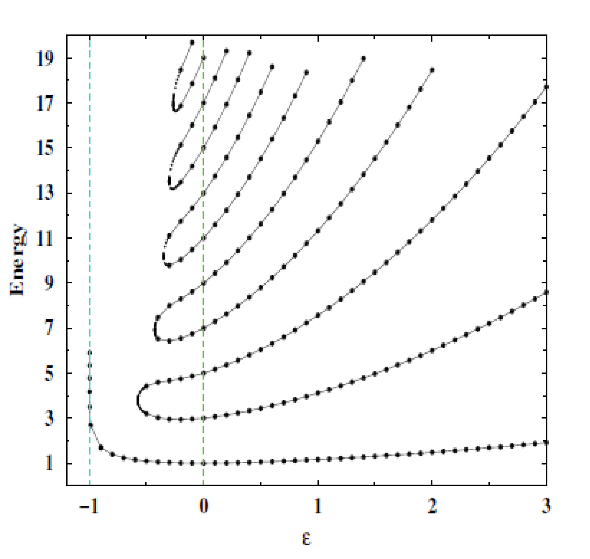
Figure 1: Energy levels of the parametric family of Hamiltonians $H=p^{2}+x^{2}(ix)^{\varepsilon}$ ($\varepsilon\,{\rm real}$). When $\varepsilon\geq 0$, the eigenvalues are all real and positive, and increase with increasing $\varepsilon$. When $\varepsilon$ decreases below $0$, the eigenvalues disappear into the complex plane as complex conjugate pairs. Eventually, only one real eigenvalue remains when $\varepsilon$ is less than about $-0.57$, and as $\varepsilon$ approaches $-1$ from above, this eigenvalue becomes infinite.

What happens if we begin with the negative harmonic-oscillator eigenvalues at $\varepsilon=0$, instead of the positive eigenvalues, and smoothly increase or decrease $\varepsilon$? Do the eigenvalues remain real and negative? More generally, what happens if we begin with the negative eigenvalues that one obtains when $\varepsilon=2N-2$ ($N=1,\,2,\,3,\,\ldots$) [see (6)], and then vary $\varepsilon$? Do the eigenvalues all remain real and negative? We will see that if we begin with the negative-real eigenvalues at $\varepsilon=2N-2$, the smallest-negative eigenvalue remains real and negative but only for a finite range of $\varepsilon$ and not an infinite range of $\varepsilon$:

$$\frac{4N-6}{3}<\varepsilon<4N-2\qquad(N=1,\,2,\,3,\,\ldots).$$ (6)

As $\varepsilon$ approaches the upper and lower edges of the $N$th region, this eigenvalue approaches $-\infty$. The larger-negative eigenvalues eventually become complex. When $\varepsilon\neq 2N-2$, there are always a finite number of real negative eigenvalues and an infinite number of complex eigenvalues. The behaviors of the eigenvalues in the first three regions $N=1,\,2,\,3$ are shown in Fig. 2.

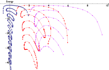
Figure 2: Negative eigenvalues of the Hamiltonian $H=p^{2}+x^{2}(ix)^{\varepsilon}$ ($\varepsilon$ real) in the first three regions of $\varepsilon$, $-2/3<\varepsilon<2$ (dots), $2/3<\varepsilon<6$ (squares), and $2<\varepsilon<10$ (diamonds), corresponding to $N=1$, $2$, and $3$ in (6). (In the electronic version the $N=1$, $N=2$, and $N=3$ eigenvalues are plotted as blue dots, red squares, and purple diamonds, respectively.) At $\varepsilon=0,\,2,\,4$ the eigenvalues are the exact negatives of the conventional positive eigenvalues of the Hermitian Hamiltonians $H=p^{2}+x^{2}$, $H=p^{2}+x^{4}$, $H=p^{2}+x^{6}$. When $\varepsilon\neq 2N-2$, there are only a finite number of real negative eigenvalues and the remaining eigenvalues are complex.

This paper is organized as follows: In Sec. II we explain the role of the Stokes wedges for the $\mathcal{P}\mathcal{T}$-symmetric negative-eigenvalue problem for the Hamiltonian in (5). Then in Sec. III we use WKB to obtain accurate numerical approximations to the real eigenvalues. We show that WKB provides a clear explanation for why the eigenvalues in the $N$th region diverge at the lower and upper ends of the region, namely, that the turning points rotate out of the Stokes wedges in which the eigenvalue problem is posed. In Sec. IV we make some brief concluding remarks.

II Stokes wedges

To construct a $\mathcal{P}\mathcal{T}$-symmetric extension of the Hamiltonian $H$ in (5), we must recall the effects of $\mathcal{P}$ and $\mathcal{T}$ on the complex coordinate $x$. Under space reflection (parity) the coordinate $x$ changes sign, $\mathcal{P}:\,x\to-x$, and under time reversal $i$ changes sign, $\mathcal{T}:\,x\to x^{*}$. Therefore, under the combined $\mathcal{P}\mathcal{T}$ operation the complex coordinate $x$ is reflected about the imaginary axis. Thus, as the Schrödinger eigenvalue problem

$$-\psi^{\prime\prime}(x)+x^{2}(ix)^{\varepsilon}\psi(x)=E\psi(x)$$ (7)

is posed in the cut complex-$x$ plane, the requirement of $\mathcal{P}\mathcal{T}$ symmetry demands that the cut lie on the imaginary-$x$ axis. We take the cut to lie on the positive-imaginary axis (see Fig. 3) because for the usual positive-eigenvalue solutions to the Hamiltonian (5) the cut was originally taken to lie on the positive-imaginary axis R3 .

The eigenvalue problem (7) is then posed on a three-sheeted Riemann surface. As is shown in Fig. 3, on sheet $-1$ the complex argument of $x$ lies in the range $-\frac{7}{2}\pi<{\rm arg}\,x<-\frac{3}{2}\pi$, on sheet $0$ (the principal sheet) the range is $-\frac{3}{2}\pi<{\rm arg}\,x<\frac{1}{2}\pi$, and on sheet $1$ the range is $\frac{1}{2}\pi<{\rm arg}\,x<\frac{5}{2}\pi$.

Figure 3: Configuration of Stokes wedges and turning points for the case $N=1$. As $\varepsilon$ increases, the right wedge (solid lines), which begins on sheets 0 and 1, rotates clockwise and downward, as indicated by the solid double arrow and the wedge lies entirely on sheet 0 when $\varepsilon>1$. The wedge becomes thinner as it rotates, and its opening angle vanishes as $\varepsilon\to\infty$; at this point the center of the wedge lies at the angle $-\pi/2$. The behavior of the left wedge (dotted lines) mirrors the behavior of the right wedge, and its rotation is indicated by the double dotted arrow. The eigenvalue problem associated with these wedges has real eigenvalues when the turning points lie inside the wedges, and this occurs only when $-2/3<\varepsilon<2$.

Using the techniques described in detail in Ref. R3 , we identify the Stokes wedges in which the boundary conditions of the differential-equation eigenvalue problem are imposed. The centers of the right and left wedges are

$$\theta_{\rm center-R}=\frac{4}{4+\varepsilon}\pi-\frac{1}{2}\pi,\qquad\theta_{\rm center-L}=-\frac{4}{4+\varepsilon}\pi-\frac{1}{2}\pi.$$ (8)

These angles lie on the principal sheet and are $\mathcal{P}\mathcal{T}$-symmetric reflections of one another.

The opening angle of the wedges is given by

$$\theta_{\rm opening~{}angle}=\frac{2}{4+\varepsilon}\pi.$$ (9)

The angular locations of the upper and lower edges of the right wedge are

$$\theta_{\rm upper~{}edge-R}=\frac{5}{4+\varepsilon}\pi-\frac{1}{2}\pi,\qquad\theta_{\rm lower~{}edge-R}=\frac{3}{4+\varepsilon}\pi-\frac{1}{2}\pi,$$ (10)

and the angular locations of the upper and lower edges of the left wedge are

$$\theta_{\rm upper~{}edge-L}=-5\frac{5}{4+\varepsilon}\pi-\frac{1}{2}\pi,\qquad\theta_{\rm lower~{}edge-L}=-\frac{3}{4+\varepsilon}\pi-\frac{1}{2}\pi.$$ (11)

Note that the right wedge extends onto sheet $1$ and the left wedge extends onto sheet $-1$ until $\varepsilon$ becomes larger than $1$. The wedges become thinner and rotate downward as $\varepsilon$ increases, and as $\varepsilon\to\infty$, the two wedges become infinitely thin and approach $-\mbox{$\textstyle{\frac{1}{2}}$}\pi$.

For positive eigenvalues $E$, the turning points satisfy the equation $x^{2}(ix)^{\varepsilon}=E$ and the turning points lie on the real axis when $\varepsilon=0$. However, for negative eigenvalues $E=-|E|$, the turning points satisfy the equation

$$(ix)^{2+\varepsilon}=-|E|.$$ (12)

There is a pair of turning points located at the angles

$$\theta_{\rm turning~{}point-R}=\frac{2}{2+\varepsilon}\pi-\frac{1}{2}\pi,\qquad\theta_{\rm turning~{}point-L}=-\frac{2}{2+\varepsilon}\pi-\frac{1}{2}\pi.$$ (13)

Thus, when $\varepsilon=0$, the turning points lie on the imaginary axis and sit in the center of each wedge.

As $\varepsilon$ varies, both the wedges and the turning points rotate in the complex-$x$ plane, but the turning points rotate faster than the wedges. Thus, the turning points in (13) only lie inside of the wedges for the range of $\varepsilon$

$$-\frac{2}{3}<\varepsilon<2.$$ (14)

Therefore, as we explain in Sec. III, the WKB asymptotic estimate of the eigenvalues breaks down when $\varepsilon$ is not in this range. This phenomenon of turning points entering and leaving wedges is discussed in Ref. R21 ; this phenomenon does not occur for the case of the positive eigenvalues discussed in Ref. R3 .

There are infinitely many solutions to the turning-point equation (12). The angular distance between successive turning points is $\frac{2}{2+\varepsilon}\pi$. The integer $N$ labels the turning points and the $N$th pair of turning points lies at the angles

$$\theta_{\rm turning~{}points}=\pm\frac{2N}{2+\varepsilon}\pi-\frac{1}{2}\pi\qquad(N=1,\,2,\,3,\,\ldots).$$ (15)

The $N$th turning point lies in the $N$th pair of wedges given by

$$\theta_{\rm upper~{}edges} = \pm\frac{2N+3}{4+\varepsilon}\pi-\frac{1}{2}\pi\qquad(N=1,\,2,\,3,\,\ldots),$$

$$\theta_{\rm lower~{}edges} = \pm\frac{2N+1}{4+\varepsilon}\pi-\frac{1}{2}\pi\qquad(N=1,\,2,\,3,\,\ldots).$$ (16)

The condition that the $N$th turning point lies in the $N$th pair of wedges is (6). [The region of $\varepsilon$ in (14) corresponds to $N=1$.] All the turning points and wedges collapse to the angle $-\mbox{$\textstyle{\frac{1}{2}}$}\pi$ as $\varepsilon\to\infty$.

III WKB calculation of the negative eigenvalues

We can use WKB to obtain an approximate formula for the $n$th eigenvalue in the $N$th range of $\varepsilon$. To do so, we simply evaluate the WKB quantization formula

$$\int_{x_{1}}^{x_{2}}dx\,\sqrt{E_{n}-V(x)}\sim(n+1/2)\pi\qquad(n\to\infty),$$ (17)

where the path of integration runs from the left turning point to the right turning point. The result is

$$E_{n}=-\left[-\frac{\sqrt{\pi}\left(n+\mbox{$\textstyle{\frac{1}{2}}$}\right)\Gamma\left(\frac{3}{2}+\frac{1}{\varepsilon+2}\right)}{\Gamma\left(1+\frac{1}{\varepsilon+2}\right)\cos\left(\frac{2N\pi}{\varepsilon+2}\right)}\right]^{(4+2\varepsilon)/(4+\varepsilon)}.$$ (18)

Note that this formula breaks down when $\varepsilon$ approaches the lower and upper endpoints in (6) because the cosine vanishes at these points.

We have computed the eigenvalues in the $N$th region ($N=1,\,2,\,3$) numerically by integrating along the centers of the wedges and matching at the origin. This matching requires that the path go around the branch point at the origin, and thus the procedure is reminiscent of the toboggan contours studied by Znojil R22 . The numerical values of the eigenvalues are compared with the WKB prediction in (18) in Fig. 4 for $N=1$, Fig. 5 for $N=2$, and Fig. 6 for $N=3$. Note that WKB is most accurate when the turning points lie exactly in the centers of the wedges. When the turning points do not lie in the centers of the wedges, the accuracy of the WKB approximation at first increases with increasing $n$, but the accuracy eventually decreases and the WKB approximation fails entirely when the eigenvalues become complex.

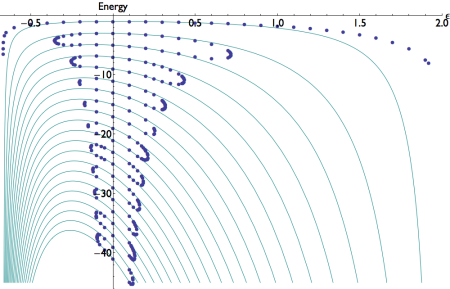
Figure 4: Comparison of the negative eigenvalues in the $N=1$ region of $\varepsilon$, $-2/3<\varepsilon<2$, with the WKB asymptotic formula (18) for the eigenvalues. The eigenvalues are plotted as dots (colored blue in the electronic version) and the WKB formula is plotted as solid curves (colored light blue in the electronic version). At $\varepsilon=0$ the eigenvalues are exactly $-1,\,-3,\,-5,\,\ldots$, which are the negatives of the conventional positive eigenvalues of the harmonic-oscillator Hamiltonian $H=p^{2}+x^{2}$. Note that when $\varepsilon\neq 0$ there are only a finite number of negative eigenvalues.

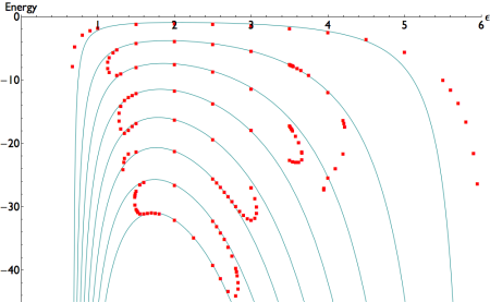
Figure 5: Comparison of the negative eigenvalues in the $N=2$ region of $\varepsilon$, $2/3<\varepsilon<6$, with the WKB asymptotic formula for these eigenvalues. The eigenvalues are plotted as squares (colored red in the electronic version) and the WKB formula is plotted as solid curves (green in the electronic version). At $\varepsilon=2$ the eigenvalues are exactly the negatives of the conventional quartic anharmonic-oscillator Hamiltonian $H=p^{2}+x^{4}$. When $\varepsilon\neq 2$ there are only a finite number of negative eigenvalues. The snake-like behavior of the eigenvalues as functions of $\varepsilon$ is similar to what was found in Ref. R21 for some positive-eigenvalue problems.

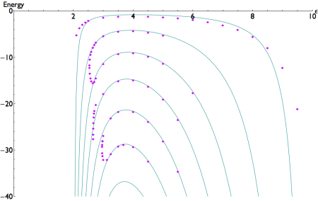
Figure 6: Comparison of the negative eigenvalues in the $N=3$ region of $\varepsilon$, $2<\varepsilon<10$, with the WKB asymptotic formula for these eigenvalues. The eigenvalues are plotted as diamonds (colored purple in the electronic version) and the WKB formula is plotted as solid curves (green in the electronic version). At $\varepsilon=4$ the eigenvalues are exactly the negatives of the conventional positive eigenvalues of the sextic anharmonic-oscillator Hamiltonian $H=p^{2}+x^{6}$. When $\varepsilon\neq 4$ there are only a finite number of negative negative eigenvalues.

IV Concluding remarks

In this paper we have studied the behavior of the negative-energy eigenvalues of the Hamiltonian (5) as functions of $\varepsilon$. We find that the behavior of the negative-energy eigenvalues is completely different from that of the positive-energy eigenvalues. The positive-energy eigenvalues remain real and positive on the infinite interval $\varepsilon\geq 0$, and this is because the turning points never leave the Stokes wedges associated with this eigenvalue problem. However, the negative-energy eigenvalues occur in an infinite sequence of finite intervals, as in (6), and at the edges of these intervals the turning points leave the Stokes wedges. Moreover, while the positive-energy spectrum is entirely real, the negative-energy spectrum eventually becomes complex when the energy becomes sufficiently negative except at the isolated values $\varepsilon=2N-2$.

The smooth behavior of the positive energies and the choppy behavior of the negative energies of the Hamiltonian (5) bears a striking similarity to the behavior of the Gamma function $\Gamma(z)$ for positive and negative $z$. The function $\Gamma(z)$ is smooth and positive for all positive $z$. However, when $z$ is negative, $\Gamma(z)$ is only smooth on finite intervals of unit length, and at the edges ot these intervals $\Gamma(z)$ is singular. The finite intervals of $\varepsilon$ that we have found in this paper are also remarkably similar to the intervals of $[1/K,4K]$ ($K=1,\,2,\,3,\,\ldots$) found in Ref. R23 , which presented a study of spontaneously broken classical $\mathcal{P}\mathcal{T}$ symmetry, and the intervals found in Ref. R21 , which re-examined the work in Ref. R23 at the quantized level.

To underscore the dramatic differences between the positive-energy and the negative-energy properties of the Hamiltonian (5), we examine the Hamiltonian at the classical level. In Figs. 7 and 8 we plot the classical trajectories in complex momentum space for $\varepsilon=1,\,3,\,5$. (We use momentum space here rather than coordinate space because in $p$ space there are always two turning points while in $x$ space the number of turning points varies with $\varepsilon$ R24 .) Note that the positive-energy classical trajectories are of uniform complexity and make simple loops around each of the turning points. In contrast, the negative-energy classical trajectories are extremely complicated, so complicated that to display them more clearly we include blow-ups of the trajectories in Fig. 8. These classical trajectories strongly suggest that at the quantum level the structure of the negative-energy sector is more complicated and far richer than that of the positive-energy sector.

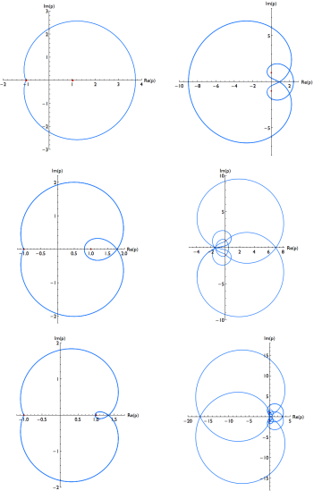
Figure 7: Comparison of the positive-energy and negative-energy classical momentum-space trajectories for the Hamiltonian (5) for $\varepsilon=1,\,3,\,5$. The positive-energy trajectories are relatively uncomplicated and make simple loops around the two turning points (red dots). The negative-energy trajectories are quite complicated (blow-ups of these trajectories are shown in Fig. 8). The contrast in complexity between the positive- and negative-energy trajectories is striking and suggests strongly that the negative-energy sector of the theory defined by the Hamiltonian (5) is richer and more elaborate than the positive-energy sector.

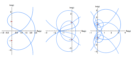
Figure 8: Blow-ups of the complicated portions of the negative-energy momentum space in Fig. 7.

We acknowledge conversations with J. Watkins. CMB is grateful to the Graduate School at the University of Heidelberg for its hospitality and he thanks the U.K. Leverhulme Foundation and the U.S. Department of Energy for financial support. Numerical calculations of eigenvalues were done using Mathematica.

References

- (1) C. M. Bender and A. Turbiner, Phys. Lett. A 173, 442 (1993).
- (2) C. M. Bender and S. A. Orszag, Advanced Mathematical Methods for Scientists and Engineers (McGraw Hill, New York, 1978).
- (3) C. M. Bender and S. Boettcher, Phys. Rev. Lett. 80, 5243 (1998).
- (4) C. M. Bender, S. Boettcher, and P. N. Meisinger, J. Math. Phys. 40, 2201 (1999).
- (5) C. M. Bender, Reps. Prog. Phys. 70, 947 (2007).
- (6) P. E. Dorey, C. Dunning, and R. Tateo, J. Phys. A: Math. Gen. 34, L391 (2001) and 34, 5679 (2001).
- (7) P. E. Dorey, C. Dunning, and R. Tateo, J. Phys. A: Math. Gen. 40, R205 (2007).
- (8) C. M. Bender, D. C. Brody, and H. F. Jones, Phys. Rev. Lett 89, 270401 (2002).
- (9) J. Rubinstein, P. Sternberg, and Q. Ma, Phys. Rev. Lett. 99, 167003 (2007).
- (10) A. Guo, G. J. Salamo, D. Duchesne, R. Morandotti, M. Volatier-Ravat, V. Aimez, G. A. Siviloglou, and D. N. Christodoulides, Phys. Rev. Lett. 103, 093902 (2009).
- (11) C. E. Rüter, K. G. Makris, R. El-Ganainy, D. N. Christodoulides, M. Segev, and D. Kip, Nat. Phys. 6, 192 (2010).
- (12) K. F. Zhao, M. Schaden, and Z. Wu, Phys. Rev. A 81, 042903 (2010).
- (13) Y. D. Chong, L. Ge, and A. D. Stone, Phys. Rev. Lett. 106, 093902 (2011).
- (14) Z. Lin, H. Ramezani, T. Eichelkraut, T. Kottos, H. Cao, and D. N. Christodoulides, Phys. Rev. Lett. 106, 213901 (2011).
- (15) L. Feng, M. Ayache, J. Huang, Y.-L. Xu, M.-H. Lu, Y.-F. Chen, Y. Fainman, and A. Scherer, Science 333, 729 (2011).
- (16) J. Schindler, A. Li, M. C. Zheng, F. M. Ellis, T. Kottos, Phys. Rev. A 84, 040101(R) (2011).
- (17) C. Zheng, L. Hao, and G. L. Long, arXiv:1105.6157 [quant-ph] (2011).
- (18) M. Fagotti, C. Bonati, D. Logoteta, P. Marconcini, and M. Macucci, Phys. Rev. B 83, 241406(R) (2011).
- (19) A. Szameit, M. C. Rechtsman, O. Bahat-Treidel, and M. Segev, Phys. Rev. A 84, 021806(R) (2011).
- (20) S. Bittner, B. Dietz, U. Günther, H. L. Harney, M. Miski-Oglu, A. Richter, and F. Schäfer, Phys. Rev. Lett. 108, 024101 (2012).
- (21) C. M. Bender and H. F. Jones, J. Phys. A: Math. Theor. 44, 015301 (2011).
- (22) M. Znojil, Phys. Lett. A 342, 36 (2005).
- (23) C. M. Bender and D. W. Darg, J. Math. Phys. 48, 042703 (2007).
- (24) C. M. Bender and D. W. Hook, J. Phys. A: Math. Theor. 41, 244005 (2008).