Holographic Entanglement Entropy in Insulator/Superconductor Transition

Abstract

We investigate the behaviors of entanglement entropy in the holographical insulator/superconductor phase transition. We calculate the holographic entanglement entropy for two kinds of geometry configurations in a completely back-reacted gravitational background describing the insulator/superconductor phase transition. The non-monotonic behavior of the entanglement entropy is found in this system. In the belt geometry case, there exist four phases characterized by the chemical potential and belt width.

1 Introduction

The AdS/CFT correspondence [2, 3, 4, 5] provides a powerful theoretical method to study the strongly coupled systems in various fields of physics. One of the most widely investigated objects is the holographic superconductor (superfluid) [6, 7, 8, 9, 10]. The physical picture is that some gravity background will become unstable as one tunes some parameter, such as temperature for black hole and chemical potential for AdS soliton, to develop some kind of “hair”. This condensation of the “hair” induces the symmetry breaking, which results in the non-vanishing vacuum expectation value of the dual operator in the field theory side.

On the other hand, as a measurement of how a given quantum system is entangled or strongly correlated, the entanglement entropy is also considered as a useful tool for keeping track of the degrees of freedom of strongly coupled systems. Dividing a quantum system into a subsystem $\mathcal{A}$ and its complement, the entanglement entropy of $\mathcal{A}$ is known as the famous von Neumann entropy

$$S_{\mathcal{A}}=-Tr_{\mathcal{A}}(\hat{\rho}_{\mathcal{A}}\ln\hat{\rho}_{\mathcal{A}}),$$ (1)

where $\hat{\rho}_{\mathcal{A}}$ is the reduced density matrix for $\mathcal{A}$ by tracing over its complement of the total density matrix. However, the calculation of entanglement entropy for a given system is found to be very difficult except for the case in $1+1$ dimensions.

Inspired by the Bekenstein-Hawking entropy of black hole and motivated by the development of AdS/CFT correspondence, the authors in Refs. [11, 12] have presented a proposal to compute the entanglement entropy of conformal field theories (CFTs) from the minimal area surface in gravity side. Precisely, in an asymptotically anti de-Sitter (AdS) spacetime, consider a slice at constant radial coordinate $r=1/\epsilon$, which is dual to a field theory “living” on this slice with a UV cutoff labeled by the small parameter $\epsilon$. the $\epsilon\rightarrow 0$ corresponds to the UV limit of the dual field theory, which is known as the UV-IR relation [13]. Search for the minimal area surface $\gamma_{\mathcal{A}}$ in the bulk with the same boundary $\partial\mathcal{A}$ of a region $\mathcal{A}$ on that slice. The entanglement entropy of $\mathcal{A}$ with its complement is defined as the “area law”:

$$S_{\mathcal{A}}=\frac{\rm Area(\gamma_{\mathcal{A}})}{4G_{N}},$$ (2)

where $G_{N}$ is the Newton’s constant in the bulk. A proof for this proposal from the basic principle of holographic duality is given in Ref. [14] and further properties of the holographic entanglement entropy are discussed in Ref. [15].

This proposal provides an elegant and executable way to calculate entanglement entropy of a strongly coupled system which has a gravity dual. Since then a lot of works have been carried out [16, 17, 18, 19, 20, 21, 22, 23, 24] for investigating and calculating the entanglement entropy in various gravity theories. In particular, Refs. [21, 22, 23] presented the calculations of entanglement entropy for AdS soliton geometry and Ref. [24] considered the case with higher derivative corrections. Very recently, the authors of Ref. [25] have studied the entanglement entropy in the holographic metal/superconductor phase transition. It was found that the entanglement entropy in superconducting phase is always less than the one in the metal phase. The entanglement entropy is continuous, but does not smoothly cross the second order phase transition.

The holographic insulator/superconductor phase transition was first studied in Ref. [10], where the AdS soliton background [26] was used to mimic the insulator/superconductor phase transition at zero temperature. Motivated by Ref. [25] we are going to explore the behaviors of the entanglement entropy in the insulator/superconductor phase transition.

The model of the holographic insulator/superconductor phase transition is constructed in the Einstein-Maxwell-scalar theory with a negative cosmological constant in five-dimensional spacetime. After completely solving the set of coupled equations of motion, we calculate the entanglement entropy for two geometry configurations, one is a half space and the other is a belt. In both cases, we find a discontinuity in the slope of the entanglement entropy as a function of chemical potential across the phase transition. But, unlike the case of the metal/superconductor phase transition [25], after condensate, the entropy first rises as we increase the chemical potential $\mu$, arrives at its maximum at a certain chemical potential and then it decreases monotonously. For the belt geometry, there exits a so-called “confinement/deconfinement” transition controlled by belt width. Our results confirm the prediction in Ref. [22] that this phase transition must appear in any consistent gravity dual of a confining theory. So there are totally four “phases” parameterized by chemical potential $\mu$ and belt width $\ell$. The complete “phase diagram” is drawn in Figure.(8). Here we would like to address that in fact there does not exist the parameter “belt width $\ell$” in the dual field theory. When one changes $\ell$, that a new “phase” occurs in the entanglement entropy manifests a length scale of dual field theory under consideration. For example, in this paper the length scale is nothing, but the correlation length of the confining theory.

This paper is organized as follows. In Section (2), we briefly review the holographic insulor/superconductor phase transition presented in Ref. [27], and give the complete equations of motion to be solved. In Section(3), the fully back-reacted system is solved by shooting method. In Section(4) we explore the behaviors of the entanglement entropy in insulator/superconductor phase transition. The conclusions and some discussions are included in Section (5).

2 AdS Soliton Background

Let us start with the Einstein-Maxwell-complex scalar theory with a negative cosmological constant in five-dimensional spacetime

$$S=\int d^{5}x\sqrt{-g}\left(\mathcal{R}+\frac{12}{L^{2}}-\frac{1}{4}F^{\mu\nu}F_{\mu\nu}-|D\psi|^{2}-m^{2}|\psi|^{2}\right)\;,$$ (3)

where $L$ is the radius of AdS spacetime, field strength $F=dA$ and $D_{\mu}=\nabla_{\mu}-iqA_{\mu}$. When the Maxwell field and scalar field are vanishing, the above action admits an exact solution named as AdS soliton

$$ds^{2}=\frac{L^{2}dr^{2}}{r^{2}f(r)}+r^{2}(-dt^{2}+dx^{2}+dy^{2}+f(r)d\chi^{2}),\qquad f(r)=1-\frac{r_{0}^{4}}{r^{4}}\;.$$ (4)

This asymptotically AdS solution approaches to $R^{1,2}\times S^{1}$ near the boundary at $r\to\infty$. Moreover, the compactification $\chi\sim\chi+\pi L/r_{0}$ needed to avoid a conical singularity at $r=r_{0}$ gives a dual picture of a three-dimensional field theory with a mass gap, which resembles an insulator in the condensed matter physics [10]. The geometry in the $(r,\chi)$ sector just looks like a cigar with its tip at $r=r_{0}$. The temperature associated with the soliton background is zero.

In order to mimic the superconductor phase, we need the soliton solutions with nonvanishing $\psi$. Furthermore, the back reaction of the matter fields must be taken into account in order to see the difference of the holographic entanglement entropy. So we choose the ansatz as follows

$$ds^{2}=\frac{dr^{2}}{r^{2}B(r)}+r^{2}\left(-e^{C(r)}dt^{2}+dx^{2}+dy^{2}+e^{A(r)}B(r)d\chi^{2}\right),\ \ A_{t}=\phi(r),\ \ \psi=\psi(r).$$ (5)

Here we have set $L=1$ without lose of generality. We require that $B(r)$ vanishes at the tip of the soliton. And in order to obtain a smooth geometry at the tip $r_{0}$, $\chi$ should be made with an identification

$$\chi\sim\chi+\Gamma,\qquad\Gamma=\frac{4\pi e^{-A(r_{0})/2}}{r_{0}^{2}B^{\prime}(r_{0})}\;.$$ (6)

The independent equations of motion under this ansatz are given as

$$\psi^{\prime\prime}+\left(\frac{5}{r}+\frac{A^{\prime}}{2}+\frac{B^{\prime}}{B}+\frac{C^{\prime}}{2}\right)\psi^{\prime}+\frac{1}{r^{2}B}\left(\frac{e^{-C}q^{2}\phi^{2}}{r^{2}}-m^{2}\right)\psi=0\;,$$ (7)

$$\phi^{\prime\prime}+\left(\frac{3}{r}+\frac{A^{\prime}}{2}+\frac{B^{\prime}}{B}-\frac{C^{\prime}}{2}\right)\phi^{\prime}-\frac{2\psi^{2}q^{2}\phi}{r^{2}B}=0\;,$$ (8)

$$A^{\prime}=\frac{2r^{2}C^{\prime\prime}+r^{2}C^{\prime 2}+4rC^{\prime}+4r^{2}\psi^{\prime 2}-2e^{-C}\phi^{\prime 2}}{r(6+rC^{\prime})}\;,$$ (9)

$$C^{\prime\prime}+\frac{1}{2}C^{\prime 2}+\left(\frac{5}{r}+\frac{A^{\prime}}{2}+\frac{B^{\prime}}{B}\right)C^{\prime}-\left(\phi^{\prime 2}+\frac{2q^{2}\phi^{2}\psi^{2}}{r^{2}B}\right)\frac{e^{-C}}{r^{2}}=0,$$ (10)

$$B^{\prime}\left(\frac{3}{r}-\frac{C^{\prime}}{2}\right)+B\left(\psi^{\prime 2}-\frac{1}{2}A^{\prime}C^{\prime}+\frac{e^{-C}\phi^{\prime 2}}{2r^{2}}+\frac{12}{r^{2}}\right)$$

$$~{}~{}~{}~{}~{}~{}~{}~{}~{}~{}~{}~{}~{}~{}~{}~{}~{}~{}~{}~{}~{}+\frac{1}{r^{2}}\left(\frac{e^{-C}q^{2}\phi^{2}\psi^{2}}{r^{2}}+m^{2}\psi^{2}-12\right)=0\;,$$ (11)

where a prime denotes the derivative with respect to $r$. The matter fields near the boundary $r\rightarrow\infty$ should behave as

$$\psi=\frac{\psi^{(1)}}{r^{\Delta_{-}}}+\frac{\psi^{(2)}}{r^{\Delta_{+}}}+\ldots,$$ (12)

$$\phi=\mu-\frac{\rho}{r^{2}}+\ldots,$$ (13)

where $\psi^{(i)}=\langle\hat{O}_{i}\rangle,~{}i=1,2$, up to a normalization constant, and $\hat{O}_{i}$ are the corresponding dual operators of $\psi^{(i)}$ in the field theory side. The conformal dimensions of the operators are $\Delta_{\pm}=2\pm\sqrt{4+m^{2}}$. $\mu$ and $\rho$ are the corresponding chemical potential and charge density in the dual field theory, respectively.

There are only four independent parameters at the tip, i.e., $r_{0},\psi(r_{0}),\phi(r_{0}),C(r_{0})$. However, the above equations of motion have two useful scaling symmetries [27]

$$r\rightarrow\alpha r,\qquad(\chi,x,y,t)\rightarrow(\chi,x,y,t)/\alpha,\qquad\phi\rightarrow\alpha\phi,$$ (14)

$$C\rightarrow C-2\ln{\beta},\qquad t\rightarrow\beta t,\qquad\phi\rightarrow\phi/\beta.$$ (15)

These two symmetries allow us to pick any values for the position of the tip $r_{0}$ and $C(r_{0})$. In our numerical calculations, we will simply choose $r_{0}=1,C(r_{0})=0$. Furthermore, to recover the pure AdS boundary, we also need $A(\infty)=0$ and $C(\infty)=0$. In general, a solution will have a nonvanishing $C(\infty)$. In this case we will use the scaling symmetry (15) to shift $C(\infty)$ to zero.

3 Insulator/Superconductor Phase Transition

From the discussion in Section 2, for given $m^{2},q,\psi(r_{0})$, we can solve the equations of motion for the system by choosing $\phi(r_{0})$ as a shooting parameter. After solving the coupled equations, we can obtain the condensate $\langle\hat{O}\rangle$ from (12) and read off the chemical potential $\mu$ and charge density $\rho$ through (13).

In this paper we only focus on the case $m^{2}=-\frac{15}{4}$ and $q=2$. It is well known that in five-dimensional spacetime, when $-4<m^{2}<-3$, the scalar field admits two different quantizations related by a Legendre transform [28]. $\psi^{(i)}$ can either be identified as a source or an expectation value. In this paper we set $\psi^{(1)}=0$ and consider $\psi^{(2)}$ acting as the vacuum expectation value of the operator $\hat{O}_{2}$.

It is convenient to make a coordinate transformation from $r-$coordinate to $z-$coordinate by defining $z=1/r$. Therefore, the infinite boundary is now at $z=0$ and the soliton tip sits at $z_{0}=1/r_{0}=1$. Figure(1) exhibits a typical solution, where $A(z)$ and $B(z)$ are two metric functions, and $\psi(z)$ and $\phi(z)$ are the scalar field and static electric potential, respectively. Note that the metric functions $A(z)$ and $B(z)$ will be used in calculating the holographic entanglement entropy.

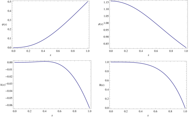
Figure 1: A typical soliton solution with nonvanishing scalar hair. Here the value of the scalar at tip is $\psi_{0}=0.5$ and the corresponding identification $\Gamma\simeq 3.0085$.

For different choices of $\psi(r_{0})$, the identification length $\Gamma$ in $\chi$ coordinate will be different. In order to compare different solutions with the same boundary behavior, we can use the symmetry (14) to set the boundary geometry the same. Taking advantage of the scaling symmetry (14), the relevant quantities scale as follows

$$\Gamma\rightarrow\frac{1}{\alpha}\Gamma,\ \ \mu\rightarrow\alpha\mu,\ \ \rho\rightarrow\alpha^{3}\rho,\ \ \langle\hat{O}_{2}\rangle\rightarrow\alpha^{\frac{5}{2}}\langle\hat{O}_{2}\rangle.$$ (16)

The combinations $\mu\Gamma$, $\rho\Gamma^{3}$ and $\langle\hat{O}_{2}\rangle^{\frac{5}{2}}\Gamma$ are all scale invariant. By using these scale invariant quantities, we can accomplish our purpose easily. As in our units setup, the identification length $\Gamma$ in the pure soliton is $\pi$, we scale all $\Gamma$ for each solution to be $\Gamma=\pi$ from now on. We should stress here that after the scaling transformation, the tip $r_{0}$ will be no longer at $r_{0}=1$.

Figure(2) reproduces the results in Ref. [27] by a slightly different manner. It shows the condensate and the charge density as functions of chemical potential. It is clear from the figure that as the chemical potential $\mu$ exceeds a critical value $\mu_{c}$ for given mass and charge, the condensation of the operators emerges. This can be identified as a superconductor (superfluid) phase. However, when less than $\mu_{c}$, the scalar field is vanishing and this can be thought of as the insulator phase, since this system has a mass gap $\sim 1/\Gamma$ due to the identification in $\chi$ direction.

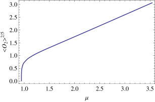
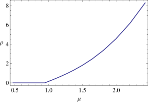
Figure 2: The condensate of operator $\langle\hat{O}_{2}\rangle$ (left plot) and the charge density $\rho$ (right plot) versus chemical potential $\mu$ respectively. Here $m^{2}=-15/4,\ q=2$ and $\Gamma$ is scaled to be $\pi$. The critical chemical potential in this case is $\mu_{c}\simeq 0.9442$. It is a typical second order phase transition which can be seen clearly from $\mu\sim\rho$ plot.

Note that it is a second order phase transition in our choice of parameters. In addition, let us mention that in the theory described by the action (3), except for the AdS soliton solution (insulator) and hairy soliton solution (superconducting soliton) mentioned above, there do exist another two solutions: the black hole solution without hair (metal phase) and black hole solution with hair (another superconducting phase). The complete phase diagram has been drawn in [27]. The details depends on the coupling constant $q$. In this paper we just focus on the case with zero temperature insultor/superconductor phase transition. As shown in [27], with our choice of parameters $m^{2}=-\frac{15}{4}$ and $q=2$, the phase transition from the insulator to the superconductor always happens. In particular, for any values of chemical potential beyond the critical one, the superconducting phase always exists.

4 Holographic Entanglement Entropy

After finding the gravitational soliton solution with full back reaction of matter fields, we are now ready to calculate the holographic entanglement entropy in this holographic model. Due to the fact that the choice of the subsystem $\mathcal{A}$ is arbitrary, we can define infinite entanglement entropies accordingly. In this paper we first consider a simple case where $\mathcal{A}$ is chosen to be a half of the total boundary space. We assume that the subsystem is defined by $x>0$ and extended in the $y$ and $\chi$ directions, where $-\frac{R}{2}<y<\frac{R}{2}\ (R\rightarrow\infty),\ 0\leq\chi\leq\Gamma$. Then the entanglement entropy can be deduced from the formula (2) as

$$S_{\mathcal{A}}^{half}=\frac{R\Gamma}{4G_{N}}\int_{r_{0}}^{\frac{1}{\epsilon}}re^{\frac{A(r)}{2}}dr.$$ (17)

For the pure AdS soliton solution, $\Gamma=\frac{\pi L}{r_{0}}$ and we can read $A(r)$ from metric (4) that $A(r)=0$. So the entropy can be easily calculated as follows.

$$S_{\mathcal{A}}^{half}=\frac{R\Gamma}{4G_{N}}\int_{r_{0}}^{\frac{1}{\epsilon}}rdr=\frac{R\Gamma}{8G_{N}}r^{2}\left.\right|_{r_{0}}^{1/\epsilon}=\frac{\pi LR}{8G_{N}r_{0}}(\frac{1}{\epsilon})^{2}-\frac{\pi LR}{8G_{N}}r_{0}=\frac{R\pi}{8G_{N}}(\frac{1}{\epsilon^{2}}-1),$$ (18)

where $r=\frac{1}{\epsilon}$ is the UV cutoff. Note that in our units setup $L=1,r_{0}=1,\Gamma=\pi$. The first term is divergent ($\epsilon\rightarrow 0$) and represents the “area law” [21]. In contrast, the second term does not depend on the cutoff and thus is physical important. In fact, this finite term is the difference between the entropy in the pure AdS soliton and the one in the pure AdS space, because in both cases the divergent part of the entanglement entropy is the same. The result in (18) implies that the entropy in the AdS soliton is less than the one in the pure AdS space.

Note that the UV behavior of $S_{\mathcal{A}}$ will not change after the operator condensation. Thus the divergent part of the entropy known as the area law will not change because this part is only sensitive to UV quantities. This can be understood from the gravity solution side, the new solution after the operator condensation still asymptotically approaches to AdS space near the AdS boundary. We can write the entanglement entropy in general in the half embedding case as

$$S_{\mathcal{A}}^{half}=\frac{R\Gamma}{4G_{N}}\int_{r_{0}}^{\frac{1}{\epsilon}}re^{\frac{A(r)}{2}}dr=\frac{R\pi}{8G_{N}}(\frac{1}{\epsilon^{2}}+s),$$ (19)

where $s$ has no divergence and $s=-1$ corresponds to the pure AdS soliton. The value of $s$ as a function of chemical potential $\mu$ in the superconductor phase is presented in Figure (3).

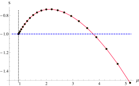
Figure 3: The entanglement entropy as a function of chemical potential in the half embedding. The solid red curve denotes the entropy in the superconductor phase, while the dashed blue line is for the pure AdS soliton solution. The entropy rises as the chemical potential $\mu$ is increased after the phase transition, arrives at its maximum at a certain $\mu$, and then decreases monotonously.

One can see from the figure that the entanglement entropy is a constant in the insulator phase. After condensate, the entropy first rises and arrives at its maximum as the chemical potential $\mu$ increases, then it decreases monotonously. Thus, from $\mu_{c}$ to a certain value of $\mu$, there exits a region where the entropies in the superconductor phase are larger than the one in the insulator phase. This behavior of entanglement entropy is quite different from the one discussed in Ref. [25], where the case for the holographic metal/superconductor phase transition has been studied in detail. It is shown that the entanglement entropy after condensate is always lower than the one in the metal phase and decreases monotonously as temperature is lowered, and the entropy as a function of temperate is found to have a discontinuous slop at the transition temperature $T_{c}$, which indicates a reduction in the number of degrees of freedom after condensate. Similarly, we here also find a discontinuity in the slope of the increasing entropy at the critical chemical potential $\mu_{c}$ indicated by the vertical dotted black line in Figure (3), which may be considered as a significant reorganization of the degrees of freedom of the system. Furthermore, this discontinuity can be regarded as the signature of the second order phase transition.

We next consider a more nontrivial geometry which is a straight belt with a finite width $\ell$ along the $x$ direction. The subsystem $\mathcal{A}$ sites on the slice $r=\frac{1}{\epsilon}$ and expends in $y$ and $\chi$ directions. The holographic dual surface $\gamma_{\mathcal{A}}$ is defined as a three-dimensional surface

$$t=0,\ \ x=x(r),\ \ -\frac{R}{2}<y<\frac{R}{2}\ (R\rightarrow\infty),\ \ 0\leq\chi\leq\Gamma.$$ (20)

$R$ is the regularized length in $y$ direction. The holographic surface $\gamma_{\mathcal{A}}$ starts from $x=\frac{\ell}{2}$ at $r=\frac{1}{\epsilon}$, extends into the bulk until it reaches $r=r_{*}$, then returns back to the AdS boundary $r=\frac{1}{\epsilon}$ at $x=-\frac{\ell}{2}$. It is easy to obtain the induced metric on $\gamma_{\mathcal{A}}$ as

$$ds^{2}=h_{ij}dx^{i}dx^{j}=\left(\frac{1}{r^{2}B(r)}+r^{2}\left(\frac{dx}{dr}\right)^{2}\right)dr^{2}+r^{2}dy^{2}+r^{2}e^{A(r)}B(r)d\chi^{2}.$$ (21)

Using the proposal (2), we need to minimize the following functional

$$S_{\mathcal{A}}[x]=\frac{R\Gamma}{2G_{N}}\int_{r_{*}}^{\frac{1}{\epsilon}}re^{\frac{A(r)}{2}}\sqrt{1+r^{4}B(r)(dx/dr)^{2}}dr.$$ (22)

We can deduce the equation of motion for the minimal surface from (22)

$$\frac{r^{5}e^{\frac{A(r)}{2}}B(r)(dx/dr)}{\sqrt{1+r^{4}B(r)(dx/dr)^{2}}}=r_{s}^{3}e^{\frac{A(r_{s})}{2}}\sqrt{B(r_{s})},$$ (23)

where $r_{s}$ is a constant.

We are interested in the case that the surface is smooth at $r=r_{*}$, i.e. $dx/dr|_{r=r_{*}}\rightarrow\infty$. This condition ensures that $r_{s}=r_{*}$. The width $\ell$ of the subsystem $\mathcal{A}$ and $r_{*}$ are connected by the relation

$$\frac{\ell}{2}=\int_{r_{*}}^{\frac{1}{\epsilon}}\frac{dx}{dr}dr=\int_{r_{*}}^{\frac{1}{\epsilon}}\frac{1}{r^{2}\sqrt{B(r)(\frac{r^{6}B(r)e^{A(r)}}{r_{*}^{6}B(r_{*})e^{A(r_{*})}}-1)}}dr.$$ (24)

Finally, we obtain the entanglement entropy as

$$S_{\mathcal{A}}=\frac{R\Gamma}{2G_{N}}\int_{r_{*}}^{\frac{1}{\epsilon}}\frac{r^{4}\sqrt{B(r)}e^{A(r)}}{\sqrt{r^{6}B(r)e^{A(r)}-r_{*}^{6}B(r_{*})e^{A(r_{*})}}}dr=\frac{R\Gamma}{4G_{N}}(\frac{1}{\epsilon^{2}}+s),$$ (25)

where the UV cutoff has been taken into consideration. However, there is also a disconnected solution describing two separated surfaces that are located at $x=\pm\frac{\ell}{2}$, respectively. This configuration is just two copies of the half embedding solution that we discussed above. So the entanglement entropy of the disconnected configuration is trivially twice of the half embedding case (19).

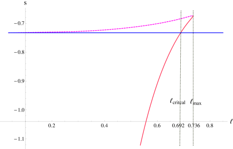
Figure 4: The entanglement entropy as a function of strip width $\ell$ for $\mu=2.2016$. The dashed magenta and solid red curves come from the connected solutions, while the solid blue one comes from the disconnected one. The lowest curve is physically favored compared with others because it has minimal entropy.

We find the behaviors of the entanglement entropy as a function of the belt width $\ell$ are quite similar for various chemical potential $\mu$ or condensation $\langle\hat{O}\rangle$. The result for $\mu=2.2016$ is shown in Figure (4) as a typical example. When $\ell>\ell_{max}$, there does not exist connected surface. The physically favored solution is replaced by the trivial disconnected one in this case. On the other hand, when $\ell<\ell_{max}$, we have three different branches of entropy for a given $\ell$ , i.e., the upper connected branch (dashed magenta curve), the lower connected branch (solid red curve) and the middle disconnected branch (solid blue line). The physical entropy is determined by the choice of the lowest one. As we can see from Figure (4), for small $\ell$, the lower connected branch is favored. However, there is a critical value $\ell_{critical}$ above which the lower connected branch is not a physical one since its entropy is larger than the one for the disconnected solution. Thus, when $\ell$ increases, a phase transition occurs as belt width $\ell=\ell_{critical}$. This is just the so-called “confinement/deconfinement” phase transition discussed intensively in Refs. [21, 22, 23, 24]. The transition can be understood as the fact that no correlation could be contributed among a distance larger than $\Gamma$ due to the mass gap $\sim 1/\Gamma$.

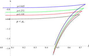
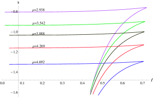
Figure 5: The entanglement entropy as a function of belt width $\ell$ for different chemical potential $\mu$. The dotted black curve is for the pure AdS soliton solution. With a fixed $\ell$, the entanglement entropy increases (left plot) and then decreases (right plot) as $\mu$ becomes large.

More numerical results for entanglement entropy are exhibited in Figure (5) with different chemical potential. For $\ell<\ell_{critical}$ at fixed chemical potential, the entropy is dominated by the connected surface and exhibits a non-trivial dependence on $\ell$. On the contrary, it is governed by the disconnected configuration and is independent of $\ell$ for $\ell>\ell_{critical}$. The fact that the phase transition always appears at critical length $\ell_{critical}$ is observed for all values of $\mu$ matches the prediction in Ref. [22] that this “confinement/deconfinemnet” phase transition must be exhibited in any consistent gravity dual of a confining theory. We find that $\ell_{max}\simeq(0.220\sim 0.237)\Gamma$ and $\ell_{critical}\simeq(0.204\sim 0.221)\Gamma$ for various chemical potentials up to $\mu=5.164$ in our numerical calculation. If the belt width is large enough ($\ell>0.237\Gamma$), the disconnected branch is always favored for all values of $\mu$. Thus, the behavior of $s$ as a function of $\mu$ for fixed $\ell$ is the same as the one shown in Figure (3).

It is helpful to slice the data in superconducting phase differently. We first study how the entropy of the system changes with chemical potential $\mu$ for fixing belt width $\ell$, which is presented in the left plot of Figure (6). It can be seen clearly that the entanglement entropy as a function of chemical potential for fixed $\ell$ has similar behavior as in the half embedding case. In particular, the purple curve in the confined phase is the same as that in Figure (3), in which $\ell\to\infty$. As the chemical potential $\mu$ increases, the entropy first rises and reaches its maximum at a certain value of chemical potential denoted as $\mu_{max}$, then it decreases monotonously. The curve will flatten out as we decrease the belt width $\ell$. The curve will finally become a line in the limit $\ell\rightarrow 0$, which can be understood from the geometric viewpoint. The minimal surface with small belt length can only probe the bulk sufficiently near the boundary $r\rightarrow\infty$ where the metric solution is nearly pure AdS. Furthermore, the value of $\mu_{max}$ also decreases as we decrease the belt width $\ell$. The values of critical belt width and entropy at the “confinement/deconfinemnet” transition point for different chemical potential are drawn in the right plot of Figure (6). The knot is a consequence of the non-monotonic behavior of the entanglement entropy.

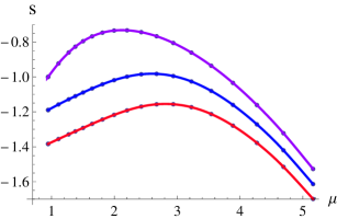
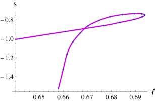
Figure 6: The entanglement entropy of the system changes with chemical potential $\mu$ for fixing belt width $\ell$ (left plot). The red curve is for $\ell=0.52<\ell_{crtical}$ and the blue one for $\ell=0.57<\ell_{critical}$. The purple curve is for sufficiently large $\ell>\ell_{max}$ in the confining phase. The right plot presents the behavior of entropy as a function of belt width at critical point of the “confinement/deconfinement” transition for different chemical potential.

In the deconfinement phase with $\ell<0.221\Gamma$, the connected branch appears, so the quantitative behavior of $s(\mu,\ell)$ changes. In order to measure the degrees of freedom at energy scale $\sim 1/\ell$ in this situation, we would like to calculate the so-called entropic c-function first introduced in Ref. [21]

$$c(\ell)=\ell^{3}\frac{ds(\ell)}{d\ell}.$$ (26)

The entropic c-function as a function of belt width $\ell$ for a fixed $\mu$ is plotted in Figure (7). Just as it is expected, the value of $c$ decreases monotonically as we increase the belt width $\ell$. Due to the appearance of mass gap $\sim 1/\pi$, the c-function jumps to zero at the critical width $\ell_{critical}$ ($\ell_{critical}\simeq 0.661$ in Figure (7)) and keeps vanishing for larger $\ell$. This is just the reason that one calls the phase transition mentioned above the “confinement/deconfinement” phase transition [21, 22, 23, 24]. We also show the change of entropic c-function as we tune the value of chemical potential for a fixed small $\ell$ in Figure (7). We can also see from the figure the non-monotonic behavior with the increment of chemical potential. Furthermore, the curve becomes flat as we decrease the belt width $\ell$. It can be expected that the curve will finally become a line in the limit $\ell\rightarrow 0$ from the perspective of gravity side. The behavior of entropic c-function as a function of chemical potential for a fixed small $\ell$ is quite qualitatively similar to the entropy in Figure (6). The key difference here is that the entropy increases as we increase the belt width, while the c-function decrease for fixed chemical potential. But an important feature we observed here is that in both phases, “confinement and deconfinement phases”, the entanglement entropy is always non-monotonic in the superconducting phase.

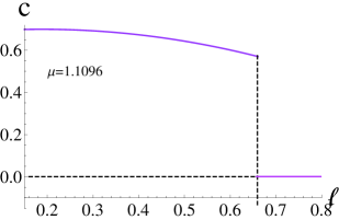
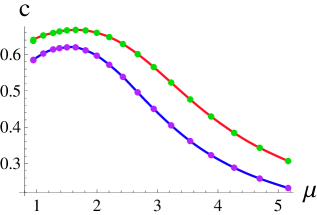
Figure 7: The entropic c-function as a function of belt width $\ell$ for $\mu=1.1096$ (left plot) and of chemical potential $\mu$ at fixed $\ell=0.5$ (right upper curve) and $\ell=0.6$ (right down curve), respectively.

To summarize, there do totally exist four phases probed by the entanglement entropy for a belt geometry for this holographic system, i.e., the confinement/deconfinement insulator phase, and confinement/deconfinement superconductor phase. These phases are characterized by the chemical potential and belt width. In particular, the belt width controls the “confinement/deconfinement” phase transition. Strictly speaking, the term phase transition here is inappropriate since the system itself, i.e., the state of the boundary field theory, does not change at all as one changes the belt width $\ell$. However, this behavior is reminiscent of many thermodynamic phase transitions in holographic calculations (see, for example Refs. [29, 30]) and so here we adopt the terminology “phase transition” to convey this picture as in the literature [21, 22, 23, 24]. Then one can draw the “phase diagram” as in Figure (8) for the system. The left part of the diagram is not new but just the one for the pure AdS soliton case which has been studied in Ref. [21]. In the superconductor phase, we find a non-trivial phase boundary between the confinement and deconfinement phases. In this sense our work is a generalization of Refs. [21, 22, 23, 24] to the superconducting soliton solution.

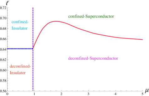
Figure 8: The “phase diagram” of entanglement entropy for a belt geometry in the holographic insulator/superconductor model for $m^{2}=-\frac{15}{4}$, $q=2$, and $\Gamma=\pi$. The phase boundary between the confinement phase and deconfinement phase is denoted by the dotted blue line and solid red curve, while the insulator phase and superconductor phase are separated by the vertical dashed line.

The non-monotonic behavior of the entanglement entropy in the superconductor phase looks strange at first glance. It is quite different from the case in the metal/superconductor transition [25], in which the result of the entanglement entropy decreasing as the temperature is lowered agrees with the fact that more degrees of freedom will be condensed in lower temperature. In our case, one can see from Figure (6) and Figure (7) that the behavior of both entropy and entropic c-function can be affected by belt width. However, the belt width $\ell$ does not play the essential role for the non-monotonic behavior. As we observed above, the non-monotonic behavior occurs in both the confinement and deconfinement superconducting phases.

Due to the lack of the knowledge of the dual field theory in the “bottom-up” approach, we do not know the details of the microscopic degrees of freedom and thus it is quite difficult to give a definite interpretation of the non-monotonic behavior of the entanglement entropy in the holographic insulator/superconductor phase transition. In order to understand the numerical result, however, we here try to give a simple physical picture as follows. Note that the entanglement entropy as a function of temperature near the critical temperature $T_{c}$ shows the same behavior in s-wave and p-wave holographic metal/superconductor models [25, 31]. The metal phase can be thought of as the one filled with free charge carriers, such as electrons. At the critical temperature the condensate turns on and the free charge carriers are continuously condensed to a certain microstate as temperature is lowered. As a result, the entanglement entropy in the superconducting phase is always less than the one in the metal phase and decreases monotonically as temperature is lowered. In contrast, the insulator phase can be considered as having a little degrees of freedom and almost all charge carriers are bound and can not move freely. This is due to the appearance of a mass gap $\sim 1/\Gamma$ which is the crucial distinction between the holographic metal/superconductor and insulator/superconductor transition. At the beginning of the phase transition the condensate emerges. Thus, a new kind of charge carriers (some quasi-particles like cooper pairs) that can move unconstrained make contribution to the degrees of freedom, which leads to the increase of the entanglement entropy. When the chemical potential is enough large, however, all bounded carriers are condensed to form cooper pairs. The system in this case is full of “cooper pairs” and thus is an ordered state seen from momentum space. As a result, the number of degrees of freedom now are even less than the one in the insulator phase. The above argument may account for the non-monotonic behavior of the entanglement entropy in the insulator/superconductor phase transition.

To further understand the non-monotonic behavior of the entanglement entropy in the insulator/superconductor phase transition, it might be helpful to recall the microscopic model presented in [10], where the authors wanted to compare the holographic insulator/superconductor transition with high-$T_{c}$ cuprates, in particular with the RVB (resonating valence bond) scenario of high-$T_{c}$ electron doped cuprates (e.g., Nd_2-xCe_xCuO₄). The phase diagrams for both systems are quite similar. The high-$T_{c}$ cuprate at $x=0$ (in the under-doped region, here $x$ stands for the electron doping) is the antiferromagnetic insulator. By doping holes, one frustrates the antiferromagnetic order and eventually destroys it. Beyond some critical doping $x_{c}$, the superconducting ground state emerges. The physics of the under-doped cuprates is well-described by the t-J model [10]. In the slave-boson (SU(2) slave-boson) approach, the electron operators can be decomposed into bosonic and fermionc parts, called holons and spinons, respectively. In the confined insulator phase, spinons and holons are completely glued together. At the beginning of phase transition, the holons get condensed and the degrees of spinons might be released. This might be the reason that the entanglement entropy increases compared to the case in the insulator phase. When the electron doping continues to increase (chemical potential gets large enough in the holographic insulator/superconudctor phase transition), the spinons will form cooper pairs and the degrees of freedom associated with spinons get condensed. In that case, the entanglement entropy of the system is even less than the case in the insulator phase. This model might explain the non-monotonic behavior of the entanglement entropy. But one caveat should be stressed here that in the gravity setup of the holographic insulator/superconductor model, an extra scalar field which is dual to the fermion bilinear in the field side does not included [10]. But one expects that including the extra scalar field to the model will not change the background geometry very much, so that the entanglement entropy keeps the same behavior. Of course, the above discussions are just some speculations, further more deep understanding for the non-monotonic behavior of the entanglement entropy is called for.

5 Summary and Discussions

By using entanglement entropy as a probe, in this paper, we investigated the holographic insulator/superconductor phase transition in a five dimensional Einstein-Maxwell-complex scalar theory with a negative cosmological constant, we calculated the entanglement entropy of dual field theory with two kinds of geometry in the AdS boundary: one is a half space, and the other is a belt geometry with width $\ell$. In the former case, we found that there does exist a discontinuity of the slop of the entropy with respect to the chemical potential at the phase transition point. This discontinuity could be thought of as a significant reorganization of the degrees of freedom of the system and a signature of the phase transition. Beyond the critical chemical potential, we found that the entanglement entropy is not monotonic in the superconductor phase: at the beginning of the transition, the entropy increases and arrives at its maximum at a certain chemical potential, and then decreases monotonically.

In the belt geometry case, the so-called “confinement/deconfinement phase transition” happens in both the insulator and superconductor phases. As $\ell<\ell_{critical}$ the connected surface is favored and the entropy depends on belt width $\ell$ non-trivially, while as $\ell>\ell_{critical}$ the disconnected surface is favored and the entropy is $\ell$ independent. The results enhance the prediction made in Ref. [22] that this phase transition must happen in any consistent gravity dual of a confining theory. Thus, as a result, there do exist four different “phases” characterized by chemical potential $\mu$ and belt width $\ell$, in the holographic insulator/superconductor phase transition. The complete “phase diagram” is drawn in Figure (8).

We observed the non-monotonic behavior of the entanglement entropy with respect to the chemical potential $\mu$ in both the “confinement/deconfinement superconductor phases. The entanglement entropy firstly rises and reaches its maximum at a certain chemical potential and then decreases monotonically (see Figure (3) and Figure (6)). Although the entanglement entropy and entropic c-function depend on the belt width, it does not play any essential role in the non-monotonic behavior of the entanglement entropy. The non-monotonic behavior of the entanglement entropy could be thought of as a key characteristic of difference between the holographic insulator/superconductor transition and the metal/superconductor transition. In the latter case, the entanglement entropy as a function of temperature near the critical transition point always monotonically decreases as temperature is lowered [25, 31]. Clearly it would be of some interest to check whether the non-monotonic behavior of the entanglement entropy is universal in other holographic insulator/superconductor model, for example, the p-wave case [33].

In addition it is worth stressing here that we did not have a clear microscopic interpretation for the non-monotonic behavior of the entanglement entropy, but we did present some arguments which try to give a physical picture for this behavior. Needless to say, it is quite necessary to deeply understand this behavior further.

In this paper, we have limited ourselves to the choice of parameters as $\psi^{(1)}=0$, $m^{2}=-\frac{15}{4}$, and $q=2$. Note that the additional complications appear for sufficiently small charge $q$. It is worthy studying the cases with other ($m^{2},\ q$)’s and the case at finite temperature. It is also interesting to study entanglement entropy in other holographic superconductor models, such as the holographic p-wave superconductor [32, 33, 34, 35]. What’s more, it is of some interest to see the effect on the entanglement entropy of the magnetic field in the holographic superconductors [36, 37, 38]. We will leave them for future studies.

References

- [1]
- [2] J. M. Maldacena, “The large N limit of superconformal field theories and supergravity,” Adv. Theor. Math. Phys. 2, 231 (1998) [Int. J. Theor. Phys. 38, 1113 (1999)] [arXiv:hep-th/9711200].
- [3] S. S. Gubser, I. R. Klebanov and A. M. Polyakov, “Gauge theory correlators from non-critical string theory,” Phys. Lett. B 428, 105 (1998) [arXiv:hep-th/9802109].
- [4] E. Witten, “Anti-de Sitter space and holography,” Adv. Theor. Math. Phys. 2, 253 (1998) [arXiv:hep-th/9802150].
- [5] O. Aharony, S. S. Gubser, J. M. Maldacena, H. Ooguri and Y. Oz, “Large N field theories, string theory and gravity,” Phys. Rept. 323, 183 (2000) [arXiv:hep-th/9905111].
- [6] S. S. Gubser, “Breaking an Abelian gauge symmetry near a black hole horizon,” Phys. Rev. D 78, 065034 (2008) [arXiv:0801.2977 [hep-th]].
- [7] S. A. Hartnoll, C. P. Herzog and G. T. Horowitz, “Building a Holographic Superconductor,” Phys. Rev. Lett. 101, 031601 (2008) [arXiv:0803.3295 [hep-th]].
- [8] S. A. Hartnoll, C. P. Herzog and G. T. Horowitz, “Holographic Superconductors,” JHEP 0812, 015 (2008) [arXiv:0810.1563 [hep-th]].
- [9] S. S. Gubser, “Colorful horizons with charge in anti-de Sitter space,” Phys. Rev. Lett. 101, 191601 (2008) [arXiv:0803.3483 [hep-th]].
- [10] T. Nishioka, S. Ryu and T. Takayanagi, “Holographic Superconductor/Insulator Transition at Zero Temperature,” JHEP 1003, 131 (2010) [arXiv:0911.0962 [hep-th]].
- [11] S. Ryu and T. Takayanagi, “Holographic derivation of entanglement entropy from AdS/CFT,” Phys. Rev. Lett. 96, 181602 (2006) [hep-th/0603001].
- [12] S. Ryu and T. Takayanagi, “Aspects of Holographic Entanglement Entropy,” JHEP 0608, 045 (2006) [hep-th/0605073].
- [13] L. Susskind and E. Witten, “The Holographic bound in anti-de Sitter space,” hep-th/9805114.
- [14] D. V. Fursaev, “Proof of the holographic formula for entanglement entropy,” JHEP 0609, 018 (2006) [hep-th/0606184].
- [15] T. Hirata and T. Takayanagi, “AdS/CFT and strong subadditivity of entanglement entropy,” JHEP 0702, 042 (2007) [hep-th/0608213].
- [16] T. Nishioka, S. Ryu and T. Takayanagi, ‘Holographic Entanglement Entropy: An Overview,” J. Phys. A A 42, 504008 (2009) [arXiv:0905.0932 [hep-th]].
- [17] T. Albash and C. V. Johnson, “Holographic Entanglement Entropy and Renormalization Group Flow,” JHEP 1202, 095 (2012) [arXiv:1110.1074 [hep-th]].
- [18] R. C. Myers and A. Singh, “Comments on Holographic Entanglement Entropy and RG Flows,” arXiv:1202.2068 [hep-th].
- [19] J. de Boer, M. Kulaxizi and A. Parnachev, “Holographic Entanglement Entropy in Lovelock Gravities,” JHEP 1107, 109 (2011) [arXiv:1101.5781 [hep-th]].
- [20] L. -Y. Hung, R. C. Myers and M. Smolkin, “On Holographic Entanglement Entropy and Higher Curvature Gravity,” JHEP 1104, 025 (2011) [arXiv:1101.5813 [hep-th]].
- [21] T. Nishioka and T. Takayanagi, “AdS Bubbles, Entropy and Closed String Tachyons,” JHEP 0701, 090 (2007) [hep-th/0611035].
- [22] I. R. Klebanov, D. Kutasov and A. Murugan, “Entanglement as a probe of confinement,” Nucl. Phys. B 796, 274 (2008) [arXiv:0709.2140 [hep-th]].
- [23] A. Pakman and A. Parnachev, “Topological Entanglement Entropy and Holography,” JHEP 0807, 097 (2008) [arXiv:0805.1891 [hep-th]].
- [24] N. Ogawa and T. Takayanagi, “Higher Derivative Corrections to Holographic Entanglement Entropy for AdS Solitons,” JHEP 1110, 147 (2011) [arXiv:1107.4363 [hep-th]].
- [25] T. Albash and C. V. Johnson, “Holographic Studies of Entanglement Entropy in Superconductors,” arXiv:1202.2605 [hep-th].
- [26] G. T. Horowitz, R. C. Myers, “The AdS / CFT correspondence and a new positive energy conjecture for general relativity,” Phys. Rev. D59, 026005 (1998). [hep-th/9808079].
- [27] G. T. Horowitz and B. Way, “Complete Phase Diagrams for a Holographic Superconductor/Insulator System,” JHEP 1011, 011 (2010) [arXiv:1007.3714 [hep-th]].
- [28] I. R. Klebanov and E. Witten, “AdS / CFT correspondence and symmetry breaking,” Nucl. Phys. B 556, 89 (1999) [hep-th/9905104].
- [29] A. Chamblin, R. Emparan, C. V. Johnson and R. C. Myers, “Charged AdS black holes and catastrophic holography,” Phys. Rev. D 60, 064018 (1999) [hep-th/9902170].
- [30] D. Mateos, R. C. Myers and R. M. Thomson, “Holographic phase transitions with fundamental matter,” Phys. Rev. Lett. 97, 091601 (2006) [hep-th/0605046].
- [31] R. -G. Cai, S. He, L. Li and Y. -L. Zhang, “Holographic Entanglement Entropy on P-wave Superconductor Phase Transition,” arXiv:1204.5962 [hep-th].
- [32] S. S. Gubser and S. S. Pufu, “The Gravity dual of a p-wave superconductor,” JHEP 0811, 033 (2008) [arXiv:0805.2960 [hep-th]].
- [33] A. Akhavan and M. Alishahiha, “P-Wave Holographic Insulator/Superconductor Phase Transition,” Phys. Rev. D 83, 086003 (2011) [arXiv:1011.6158 [hep-th]].
- [34] R. G. Cai, Z. Y. Nie and H. Q. Zhang, “Holographic p-wave superconductors from Gauss-Bonnet gravity,” Phys. Rev. D 82 (2010) 066007 [arXiv:1007.3321 [hep-th]].
- [35] R. -G. Cai, Z. -Y. Nie and H. -Q. Zhang, “Holographic Phase Transitions of P-wave Superconductors in Gauss-Bonnet Gravity with Back-reaction,” Phys. Rev. D 83, 066013 (2011) [arXiv:1012.5559 [hep-th]].
- [36] T. Albash and C. V. Johnson, “A Holographic Superconductor in an External Magnetic Field,” JHEP 0809, 121 (2008) [arXiv:0804.3466 [hep-th]].
- [37] X. -H. Ge, B. Wang, S. -F. Wu and G. -H. Yang, “Analytical study on holographic superconductors in external magnetic field,” JHEP 1008, 108 (2010) [arXiv:1002.4901 [hep-th]].
- [38] R. -G. Cai, L. Li, H. -Q. Zhang and Y. -L. Zhang, “Magnetic Field Effect on the Phase Transition in AdS Soliton Spacetime,” Phys. Rev. D 84, 126008 (2011) [arXiv:1109.5885 [hep-th]].