Reinterpretion of Experimental Results with Basis Templates

Abstract

Experimental analysis of data from particle collisions is typically expressed as statistical limits on a few benchmark models of particular, often historical, interest. The implications of the data for other theoretical models (current or future) may be powerful, but they cannot typically be calculated from the published information, except in the simplest case of a single-bin counting experiment. We present a novel solution to this long-standing problem by expressing the new model as a linear combination of models from published experimental analysis, allowing for the trivial calculation of limits on a nearly arbitrary model. We present tests in simple toy experiments, demonstrate self-consistency by using published results to reproduce other published results on the same spectrum, and provide a reinterpretation of a search for chiral down-type heavy quarks ($b^{\prime}$) in terms of a search for an exotic heavy quark ($T$) with similar but distinct phenomenology. We find $m_{T}>419$ GeV at 95% CL, currently the strongest limits if the $T$ quark decays via $T\rightarrow Wb,T\rightarrow tZ$ and $T\rightarrow tH$.

I Introduction

Data from particle colliders may reveal new states of matter or evidence for new forms of interactions, or disprove theories of such new phenomena. When no evidence of new phenomena is seen, the experimental collaborations who collect and analyze the data communicate the non-observation in terms of statistical limits on theories which predict the new states or interactions.

The space of possible theoretical models is impossibly vast; therefore experimental results are typically communicated as limits on a few benchmark models of particular or historical interest. However, the data can provide tight constraints on many other models not included in the experimental analysis – such as models not yet constructed. One solution would be for the experiments to provide a rapid mechanism for testing new models against previously analyzed datasets. Currently, however, the experiments are not capable of (or perhaps not interested in) responding to an exhaustive list of models; furthermore, experimental re-analysis typically occurs on a timescale of weeks or months rather than hours or days. Some ideas have been proposed to smoothen this process, such as recast recast , which elegantly connects the individual experimental experts to the theoretical models, but does not remove the lengthy experimental review process and so does not provide a rapid and certain solution – the experiment may still choose to not provide limits on the requested models.

To date, it has been impossible for those outside the experimental collaborations to reinterpret the published results on benchmark models in order to set limits on new models, except in a single restrictive case. When experimental analysis is performed as a simple selection of events (e.g. atlasss ; atlaszz ), it can be imagined as a counting experiment and the information needed to derive limits on new models is often included in the experimental publication. To calculate a statistical upper limit on the number of events from a new source, $N_{\rm events}$, which is compatible with the data, all that is needed are the expected contributions from standard model (SM) backgrounds (with uncertainties) and the observed collider event yield. One can then calculate an upper limit on the production cross section of the new source, $\sigma_{\rm new}$, using

$$N_{\rm events}=\sigma_{\rm new}\times\epsilon_{\rm selection}\times\mathcal{L}$$

where $\epsilon_{\rm selection}$ is the efficiency of the experimental detection and selection and $\mathcal{L}$ is the integrated luminosity of the dataset. Reasonable methods exist for estimating $\epsilon_{\rm selection}$ pgs .

Access to only single-bin analysis for reinterpretation is an unfortunately restrictive condition, as many of the most powerful and important results are those which perform a multi-bin fit to a spectrum, taking advantage of distinct signal and background shapes (e.g. atlasbp ; atlastp ; cdftj ). Use of a multi-bin histogram can greatly improve the sensitivity, but makes reinterpretation difficult, as one needs access to the bin-to-bin correlations for all background components and each of the systematic correlations leshouches . Multi-bin data may be reinterpreted directly in terms of new theoretical models but these rely on simple detector simulation tools which may not accurately describe the reconstructed variable. It is also difficult to describe all the systematic uncertainties, especially in a multi-bin analysis where a systematic uncertainty may also distort the shape of the template. Such an approach is suited for comparing features in the data against specific new models wjjh but cannot be reliably used to to calculate realistic limits in the manner of the experimental collaborations. The result is that a large fraction of published results are unusable for reinterpretation.

A solution to this problem would be experimental publication of all the details of the limit calculation, for example the complete likelihood used to analyze the final binned data. This is not currently provided by the experiments, though there are prospects for future mechanisms hepdata ; roostats .

We present a novel solution to this problem, which allows for the reinterpretation of published limits derived from multi-bin analysis. If the binned distribution of a new theoretical model can be expressed as a linear combination of the models for which published limits exist, a simple relationship allows the calculation of the limit on the new model as a simple combination of the limits on the published models. This allows a large swath of previously un-usable experimental results to confront a nearly arbitrary space of possible models without involvement by the experiment.

In the following, we introduce ”the basis-limit hypothesis”, demonstrate its effectiveness in simple artificial scenarios, show self-consistency by using published results to reproduce other published results on the same spectrum, and provide a reinterpretation of a search for chiral down-type heavy quarks ($b^{\prime}$) in terms of a search for an exotic heavy quark ($T$) with similar but distinct phenomenology.

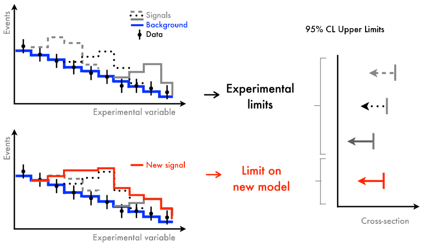
Figure 1: Upper limits on the production cross section of a new signal hypothesis can be derived if the new signal can be constructed as a linear combination of signals with existing experimental limits.

II The Basis-Limit Hypothesis

For a specific experimental dataset and background model which is analyzed using a binned likelihood in a variable $x$, there are a set of $n$ signal hypotheses described by binned distributions (“templates”) $f_{1}(x),f_{2}(x),...,f_{n}(x)$. In the case that the data prefer the background model, each signal template has an associated cross-section upper limit, which can be expressed relative to the theoretical prediction for that signal hypothesis: $\sigma^{\rm limit}_{i}/\sigma_{i}^{\rm theory}$, where $\sigma_{i}^{\rm theory}$ is the cross section used to normalize the template $f_{i}$, such that

$$N_{i}^{\rm events}=\int f_{i}(x)=\sigma_{i}^{\rm theory}\times\epsilon_{i}\times\mathcal{L},$$

and $\epsilon_{i}$ is the selection efficiency for the $i$-th signal hypothesis.

Given a new, untested signal hypothesis template, $F(x)$, which may be expressed as a linear combination of $f_{i}(x)$, as

$$F(x)=\sum_{i=0}^{n}a_{i}f_{i}(x)\ \ (a_{i}\geq 0),$$

our hypothesis is that an upper limit on the cross-section of the new signal hypothesis, $\sigma_{F}^{\rm limit}$ can be calculated from the limits ($\sigma^{\rm limit}_{i}/\sigma_{i}^{\rm theory}$) associated with each $f_{i}(x)$, as

$$\frac{\sigma_{F}^{\rm limit}}{\sigma_{F}^{\rm theory}}=\left[\sum_{i=0}^{n}a_{i}\frac{\sigma_{i}^{\rm theory}}{\sigma_{i}^{\rm limit}}\right]^{-1}$$ (1)

Stated briefly, given limits on a set of basis templates, we claim to be able to calculate limits on any new signal template which can be expressed as a linear combination of the basis templates. The idea is expressed diagrammatically in Fig 1.

III Performance in toy examples

We demonstrate the application of the basis-limit hypothesis using a simple toy scenario: a 3-bin analysis with two signal hypotheses, shown in Figure 2. The two signal templates are the basis templates and are generated with an arbitrary but equal signal cross-section, $\sigma^{\rm theory}$.

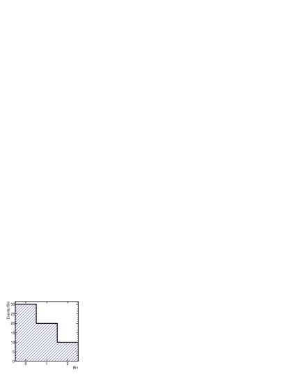
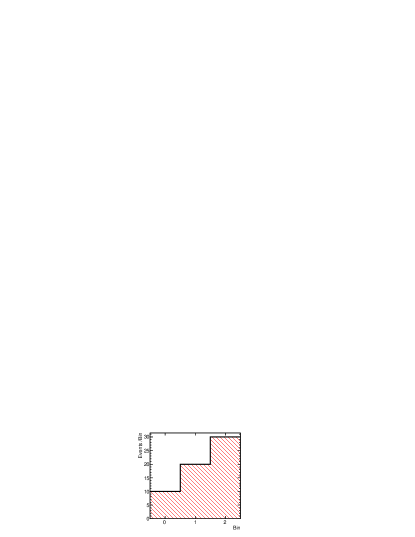
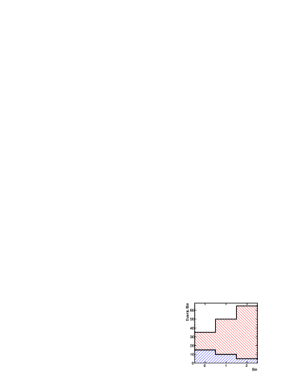
Figure 2: The example toy basis templates, $f_{1}$ (top) , $f_{2}$ (center) and a linear combination $F=0.5f_{1}+2f_{2}$. We derive a limit on the $F$ template using limits on $f_{1},f_{2}$ and the coefficients $a_{1}=0.5,a_{2}=2.0$, see Table 1.

We use the CLs technique cls1 ; cls2 to estimate cross-section upper limits on each of the basis templates relative to a flat background. For a new signal hypothesis, $F$, expressed as a linear combination of the templates, we predict the limit on $F$ using the limits on the basis templates, as shown in Equation 1. Table 1 gives an example for a single case.

Table 1: Demonstration of basis-limit application in a toy scenario. A new signal hypothesis, $F$, is formed from a linear combination of $f_{1}$ and $f_{2}$ using the coefficients $a_{i}$ (see Fig. 2). The limits ($\sigma^{\rm limit}_{i}/\sigma_{i}^{\rm theory}$) on the $f_{i}$ and the coefficients $a_{i}$ can be used to predict the limit on the new hypothesis, $F$, using Equation 1. The predicted limit is confirmed by an explicit calculation of the limit using the $F$ template.

	$f_{1}$	$f_{2}$	$F$
$a_{1}$	1.0	–	0.5
$a_{2}$	–	1.0	2.0
$\sigma^{\rm limit}_{i}/\sigma_{i}^{\rm theory}$ (meas)	0.27	0.27	0.11
$\sigma^{\rm limit}_{i}/\sigma_{i}^{\rm theory}$ (pred)	–	–	0.11

A comprehensive test, scanning many possible values of $a_{i}$, shows that the basis-limit predictions are robust in this toy example, see Fig. 3.

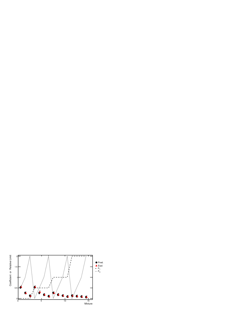
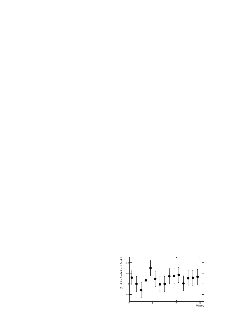
Figure 3: Tests of the basis-limit hypothesis in a toy scenario involving two signal templates, see Figure 2. For a new shape $F=a_{1}f_{1}+a_{2}f_{2}$ and a variety of $a_{1},a_{2}$ mixtures, we compare the relative upper limit on the model described by the $F$ template as calculated explicitly to that predicted by the basis-limit formula, which uses only the limits on $f_{1},f_{2}$ and the coefficients $a_{1},a_{2}$. Top pane shows the explicit and predicted upper limits for varying $a_{1},a_{2}$; bottom pane shows the difference in the explicit and predicted upper limits. Statistical uncertainties come from the pseudo-experiments required in the limit calculation.

IV Possible shortcomings

IV.1 Limited basis templates

The basis-limit hypothesis is not universally robust: it cannot be blindly applied to every published result or completely arbitrary new models. The primary limitation is whether enough example shapes are presented to form a basis to describe a new test signal.

As an extreme example to illustrate the point, consider a two-bin analysis with large background rates in each bin: $f_{bg}(x)=(10^{3},10^{3})$, but large uncertainty: $\Delta f_{bg}(x)=(10^{2},10^{2})$. A two-bin signal template with signal isolated in just one bin, $f_{1}(x)=(100,0)$, may have reasonable sensitivity, as the background uncertainty can be reduced by a fit to the observed data in the signal-depleted bin. But, if we were to make a poor choice of basis templates, in which each bin kept significant signal contributions: $f_{1}(x)=(101,99),f_{2}(x)=(99,101)$, no reduction in the background uncertainty would be possible for either signal template, leading to weak limits for both. There is no positive set of coefficients $a_{i}$ which can be combined to describe a signal hypothesis with signal isolated in one bin; these templates fail to capture the real power of the data set.

The basis-limit hypothesis implicitly assumes that the constraints on the background systematics obtained when determining limits for each of the basis templates is comparable to the constraints that would be obtained when determining limits using the new signal. This assumption is valid if, as is often the case, the background systematics are predominantly constrained in a background-rich region where both the basis template and new-signal are always small.

Another extreme example where the basis-limit hypothesis would fail is the case of a new signal template which is identical to a published template, but with larger or different systematic uncertainties.

IV.2 Approximate Efficiency Calculations

Any reinterpretation of published data in terms of a new theoretical model requires an estimate of the efficiency, $\epsilon_{selection}$ of the experiment to detect and select events from the proposed new source. While the most accurate estimate of $\epsilon_{selection}$ can only be performed by the experimental collaboration, often via use of their private official geant-based geant detector simulation programs, there are well-established public tools, such as pgs pgs , which provide estimates via a parametric simulation with reasonable accuracy ($5-20\%$ relative) in most regimes.

One application of the basis-limit approach is to build templates of the new theory using the available public simulation programs and express them as linear combinations of the published templates produced by the experiments with their private simulation programs. This incurs the same acceptable level of uncertainty in each bin as in the well-established single-bin case. The approximation of $\epsilon$ results in an approximate determination of the $a_{i}$ coefficients.

To calculate the limits on a new theory, the $\epsilon$ values are not directly needed – all that is required are the coefficients $a_{i}$ and the limits on each template $f_{i}$. If the new theory templates and the basis templates are built using the same approximate public simulation, many of the approximations may cancel. For example, if $\epsilon^{F}_{\rm approx}/\epsilon^{F}_{\rm official}=\epsilon^{f_{i}}_{\rm approx}/\epsilon^{f_{i}}_{\rm official}$ then it may be possible to calculate the $a_{i}$ without incurring approximations due to $\epsilon$. In addition, it is possible with this approach to make templates in cases when the published analysis has limits quoted for many cases but only a few example templates (e.g. atlaszp ).

V Tests with published limits

The toy scenario above demonstrates the validity of the basis-limit hypothesis when the new signal is exactly a linear combination of previously examined signals. In this section, we demonstrate the use of basis limits in realistic scenarios using published experimental results.

V.1 Same-sign dileptons at CDF

A critical test of the basis-limit hypothesis is a comparison of limits predicted using Equation 1 with limits derived by the experiment itself. This requires a pair of experimental limits which use identical datasets, selections and background models. One such pair is a search at CDF in same-sign dileptons with jets and missing energy in 6.1 fb^-1; the dataset was used to extract limits on supersymmetry cdfsssusy and same-sign top-quark pair production cdfsstops . Both analyses use $H_{T}$, the scalar sum of transverse momenta of jets and leptons, as the discriminating variable.

We form linear combinations of the SUSY templates to reproduce the same-sign top-quark templates, see Figure 4. The coefficients $a_{i}$ and the published limits on each of the SUSY templates can then be used to predict the limits on same-sign top-quark production, see Table  2. The predicted limits agree with the published results in each case.

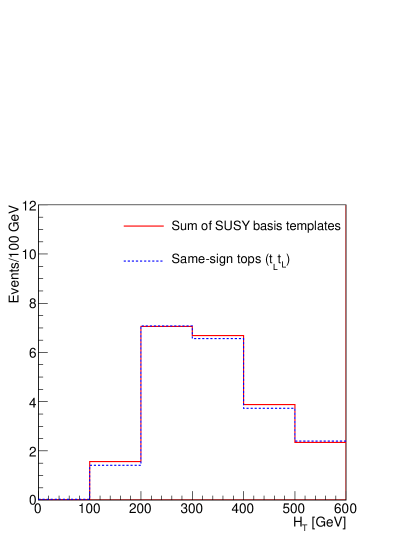
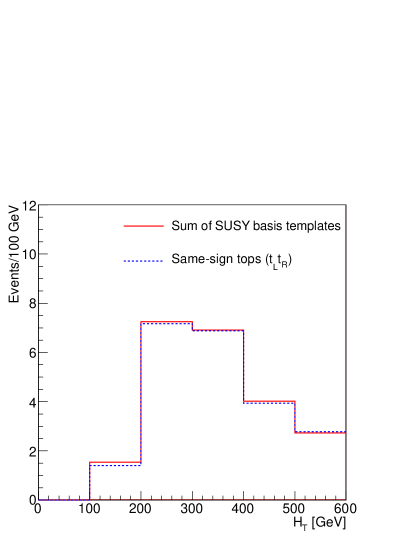
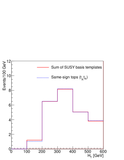
Figure 4: Distribution in event $H_{T}$ (the scalar sum of transverse momenta of jets and leptons) from same-sign top-quark pair production (blue, dashed) expressed as a linear combination of distributions from gluino-pair production and squark-pair production. Panes show show the $t_{L}t_{L}$ (top), $t_{L}t_{R}$ (center) and $t_{R}t_{R}$ (bottom) chirality configurations.

Table 2: Prediction of limits on same-sign top quark pairs in various chirality configurations derived from limits on supersymmetric production of gluinos or squarks. Coeffients of the supersymmetric particle templates are denoted by the particles and mass heirarchy, all in units of GeV. Note that coefficients are individually quoted only for the three most significant basis templates; the sum of the 30 remaining coefficients, $a_{\rm other}$ is also shown.

	$t_{L}t_{L}$	$t_{L}t_{R}$	$t_{R}t_{R}$
$a_{\tilde{g}(m=200),\chi^{+}(m=75),\chi^{0}(m=50)}$	0.061	0.074	0.098
$a_{\tilde{g}(m=300),\chi^{+}(m=150),\chi^{0}(m=100)}$	0	0	0.015
$a_{\tilde{q}(m=200),\chi^{+}(m=75),\chi^{0}(m=50)}$	0.040	0.035	0.011
$\Sigma a_{\rm other}$	0.100	0.068	0.700
Experiment Results cdfsstops [fb]	54	51	44
Our Prediction [fb]	53.7	50.9	44.1

V.2 Self-consistency test

Pairs of published experimental results with identical selection, dataset and backgrounds but distinct signal hypotheses are quite rare. However, we can probe the basis-limit performance in realistic scenarious using a self-consistency test.

In a set of $N$ signal templates, we can attempt to describe the $i$-th template using the other $N-1$ templates. Given the published limits on the $N-1$ templates, we can predict the limit on the $i$-th template and compare it to the published limit.

The ATLAS collaboration reported a search for heavy fourth-generation down-type chiral quarks ($b^{\prime}$) using 1 fb^-1 bprime . The $b^{\prime}$ decays via $tW$, leading to a final state with four $W$ bosons and two $b$ quarks, see Fig. 5. The ATLAS search makes use of a novel technique for tagging boosted $W$ bosons by searching for jet pairs with small angular separation. The analysis variable is the jet multiplicity and $W$ boson multiplicity, see Figure 6.

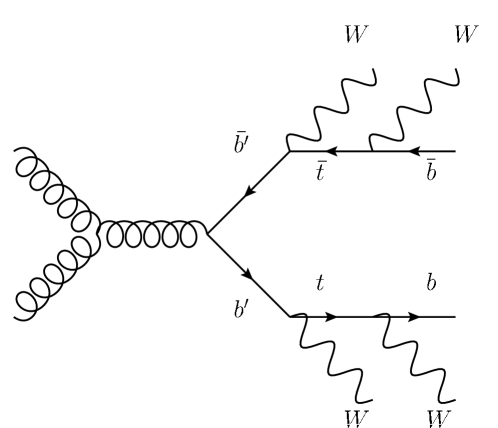
Figure 5: Pair-production of heavy down-type $b^{\prime}$ quarks with decay $b^{\prime}\rightarrow Wt$.

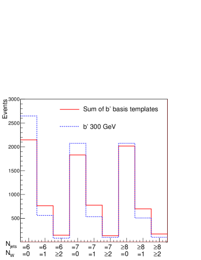
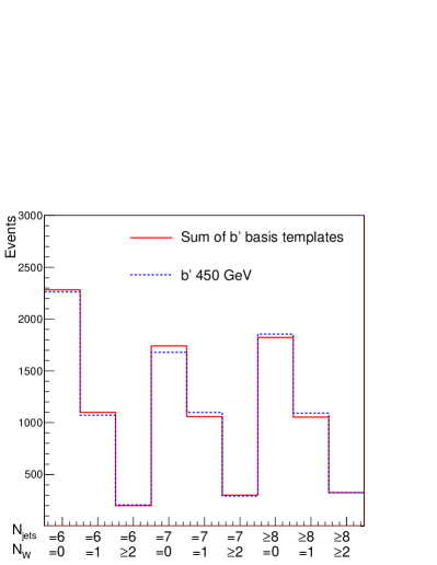
Figure 6: Jet multiplicity and hadronically-decaying $W$ multiplicity for $b\rightarrow tW$ pair production GeV (blue, dashed) expressed as a linear combination (red, solid) of distributions from other $b^{\prime}$ masses, see Table 3. Left is for $m_{b^{\prime}}=300$ GeV; right is for $m_{b^{\prime}}=450$ GeV. For the edge case of $m_{b^{\prime}}=300$ GeV, the sum of basis templates is not exact, due to the lack of templates at lower masses.

We generate $b^{\prime}\rightarrow tW$ using madgraph madgraph , use pythia pythia to model showering and hadronization, and pgs to describe the detector response. Details of the construction of the templates and the resulting limits are given in Table 3.

Figure 7 shows that the basis-limit estimation is reliable for this application. At the lower boundary, $m_{b^{\prime}}=300$ GeV, it is difficult to find coefficients which give an accurate description, see Figure 6.

Table 3: Details of the self-consistency test using $b^{\prime}\rightarrow tW$ decays at ATLAS. The template at each specific mass is expressed as a linear sum of templates at other masses; the predicted limit is then compared to the explicit calculation.

	$b^{\prime}_{300}$	$b^{\prime}_{350}$	$b^{\prime}_{400}$	$b^{\prime}_{450}$	$b^{\prime}_{500}$	$b^{\prime}_{550}$	$b^{\prime}_{600}$
$a_{b^{\prime}300}$	-	0.19	2e-3	0	0	0	0
$a_{b^{\prime}350}$	2.29	-	0.16	0	0	0	0
$a_{b^{\prime}400}$	0	1.10	-	0.23	0.03	0	0
$a_{b^{\prime}450}$	0	0.32	1.31	-	0.09	0.03	0
$a_{b^{\prime}500}$	0	0.01	0	0.35	-	0.08	0.02
$a_{b^{\prime}550}$	0	0.01	2e-3	1.10	0.40	-	0.48
$a_{b^{\prime}600}$	0	1e-3	0	0.59	1.92	1.35	-
$\sigma^{\rm limit}_{i}/\sigma_{i}^{\rm theory}$ (meas)	0.16	0.27	0.48	0.74	1.2	2.3	4.3
$\sigma^{\rm limit}_{i}/\sigma_{i}^{\rm theory}$ (pred)	0.12	0.26	0.42	0.73	1.3	2.4	4.5

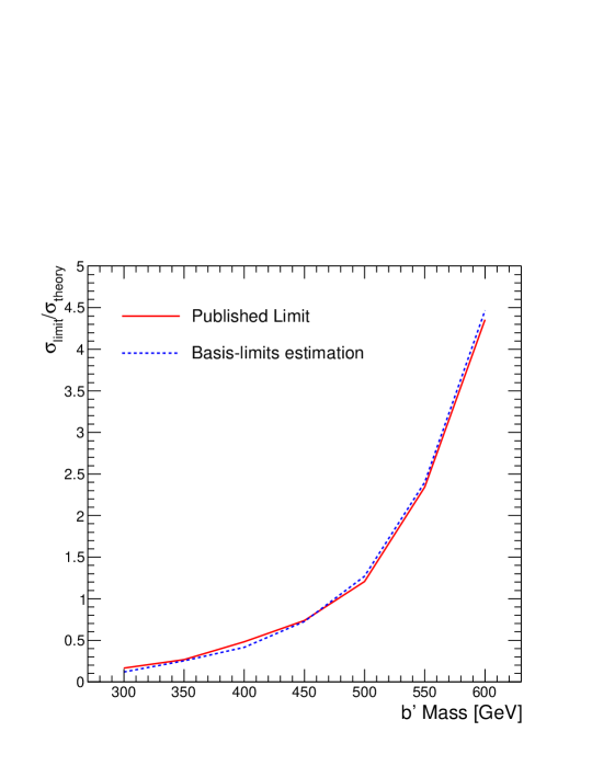
Figure 7: Prediction of limits on $b^{\prime}\rightarrow tW$ decays at ATLAS. Limits at each mass are predicted by expressing the signal model at that mass in terms of signal models at other masses; these predicted limits agree well with the limits reported by ATLAS atlasbp , see Table 3.

VI New limits on a heavy exotic quark: $T$

Having shown the validity of the basis-limit hypothesis, we provide a demonstration of the calculation of limits on an untested signal hypothesis using published experimental results.

An exotic heavy quark $T$ may decay as $T\rightarrow Wb$, $T\rightarrow tZ$, or $T\rightarrow tH$, see Fig. 8. The signature of the decay is similar to that of the $b^{\prime}$ model, involving hadronic decays of boosted bosons ($W,Z,H$) and top quarks tprime . The CMS collaboration analyzed data with 1.14 fb^-1 of integrated luminosity and excluded at 95% CL such a $T$ quark below $m_{T}=475$ GeV assuming BR($T\rightarrow tZ=100$%) cmstp . In the more likely configuration with other decay modes available and BR($T\rightarrow tZ\leq 25$%) (see  tprime ), the CMS limit would be significantly weaker, perhaps $m_{T}>250$ GeV.

We combine all decay modes together to maximize the expected yield and to be sensitive to the broader model. As before, we construct templates for $T$ as linear combinations of the existing $b^{\prime}$ templates (Fig. 9) and use Equation 1 to calculate new limits on the pair-production of $T$ at the LHC.

Table 4 shows the coefficients and calculated limits, also shown in Fig. 10. Using an approximate next-to-next-to-leading-order calculation d4xs of the $T$ production cross-section, our cross-section upper limit excludes a $T$ quark with mass $m_{T}>419$ GeV, despite the low branching ratio, BR($T\rightarrow tZ$)=15% at this $m_{T}$.

In addition, we repeat the study using only $T\rightarrow tZ$ decay modes, as these are most similar to the $b^{\prime}\rightarrow tW$ mode originally analyzed by ATLAS, see Fig 10.

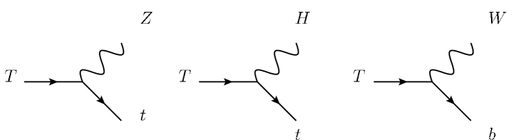
Figure 8: Decay modes of a heavy exotic quark, $T$

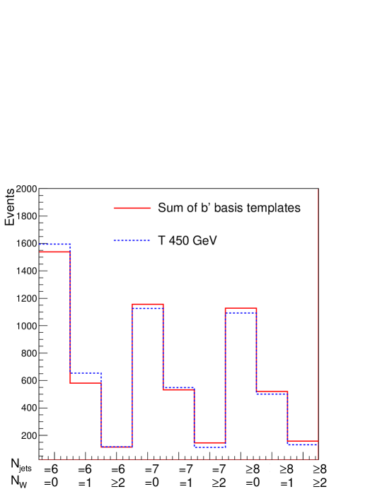
Figure 9: Jet multiplicity and hadronically-decaying $W$ multiplicity for exotic heavy quark $T$ pair production and decay with $m_{T}=450$ GeV (blue, dashed) expressed as a linear combination of distributions from $b^{\prime}\rightarrow tW$ model with varying masses, see Table 4. We include all $T$ decay modes, see Fig. 8.

Table 4: Details of the predicted limit on $T$ pair-production and decay, using basis templates from $b^{\prime}\rightarrow tW$ decays at ATLAS. We include all $T$ decay modes, see Fig. 8.

	$T_{300}$	$T_{350}$	$T_{400}$	$T_{450}$	$T_{500}$	$T_{550}$	$T_{600}$
$a_{b^{\prime}300}$	0.39	0.20	0.07	0.02	0.01	2e-3	1e-3
$a_{b^{\prime}350}$	0	0	0	0	0	0	0
$a_{b^{\prime}400}$	0	0	0	0	0	0	0
$a_{b^{\prime}450}$	0	5e-3	4e-3	3e-3	1e-3	0	0
$a_{b^{\prime}500}$	0.01	3e-3	1e-3	3e-3	0	0	0
$a_{b^{\prime}550}$	0.24	0.94	1.24	0.78	0.39	0.13	0.04
$a_{b^{\prime}600}$	4.35	2.88	1.46	1.11	0.87	0.68	0.42
$\sigma^{\rm limit}_{i}/\sigma_{i}^{\rm theory}$ (pred)	0.29	0.44	0.77	1.35	2.39	4.34	8.10
$\sigma^{\rm limit}$ [pb] (pred)	2.29	1.40	1.09	0.89	0.79	0.75	0.75

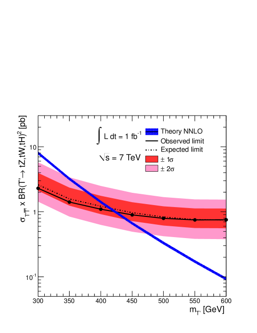
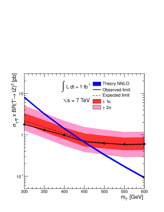
Figure 10: Upper limits at 95% CL on the production of an exotic heavy quark $T$. Top includes all decays (see Fig. 8); bottom includes only $T\rightarrow tZ$ decays. The theoretical prediction is at approximate next-to-next-to-leading-order d4xs .

VII Limitations and Generalizations

While the basis-limit hypothesis is an intuitive and effective construction, it is a heuristic formula. We do not provide its derivation from basic statistical axioms.

In some scenarios, it may fail to provide an accurate prediction of the limit on a new model, as mentioned above. Indeed, we have observed some artificial scenarios in which the basis templates have very little overlap that a bias may occur in the prediction. Some corrections may be calculable in this scenario, leading to modification of the $a_{i}$ coefficients based on the a priori overlap of the basis templates. In most cases, where the signal templates come from new physics processes with single slow-varying parameter, such as the mass of a new particle, the templates have substantial overlap and the correction is negligible.

Alternatively, we might express Eq. 1 in another form, as

$$\frac{\sigma_{F}^{\rm limit}}{\sigma_{F}^{\rm theory}}=\left[\sum_{i=0}^{n}x_{i}\kappa_{i}\right]^{-1}$$

where $x_{i}$ is the bin content of the $i$-th bin for an $n$-bin analysis, and $\kappa_{i}$ is an unknown constant which depends only on the background and data in the $i$-th bin. Rather than expressing the new signal in terms of basis templates, we could solve for the $\kappa_{i}$ given a set on $n$ limits on $n$ signal templates. This would allow the calculation of a limit on an arbitrary signal template without concern for an overlap correction as discussed above. We leave this for future investigation.

VIII Conclusions

The basis-limit hypothesis provides a tool for reinterpretting the results of experimental analysis using multi-bin data. Previously, only single-bin analyses could be reinterpreted.

Some technical hurdles remain; for example, if the published analysis uses a complex technique (such as a multi-variate analysis tool) and does not publish enough detail, then the selection cannot be reproduced. This also applies to a single-bin analysis.

Superior solutions to the one we propose here are:

• Archiving and streamlining by the experiments of published analysis, allowing for a rapid re-interpretation in terms of a new model. This has the disadvantage that it places the burden on the experiments.

• Publication by the experiments of all of the details necessary to reproduce the analysis. This has the disadvantage that it requires use of an approximate publicly-available simulation.

As neither of these are currently available, the basis-limit approach makes a wide range of results available for constraining current and future models.

We use this approach to interpret an ATLAS search for $b^{\prime}\rightarrow Wt$ to set the strongest limit on an exotic heavy quark $T$ which decays $T\rightarrow tZ,th,Wb$ at $m_{T}>419$ GeV at 95% confidence level.

IX Acknowledgements

We thank Michael Mulhearn, Jeffrey Streets, Kathy Copic, Kyle Cranmer, Nadine Amsel, Matthew Relich and Eric Albin for useful conversations, and Graham Kribs and Adam Martin for the $T$ quark model and technical support. The authors are supported by grants from the Department of Energy Office of Science and by the Alfred P. Sloan Foundation.

References

- (1) K. Cranmer and I. Yavin, JHEP 1104, 038 (2011) [arXiv:1010.2506 [hep-ex]].
- (2) ATLAS Collaboration, arXiv:1202.5520 (2012).
- (3) ATLAS Collaboration, arXiv:1203.0718 (2012).
- (4) J. Conway, http://www.physics.ucdavis.edu/c̃onway/research/software/pgs/pgs.html.
- (5) ATLAS Collaboration, arXiv:1202.6540 (2012).
- (6) ATLAS Collaboration, arXiv:1202.3389 (2012).
- (7) CDF Collaboration, arXiv:1203.3894 (2012).
- (8) S. Kraml et al., arxiv:1203.2489 (2012).
- (9) Q. H. Cao et al., J. High Energy Phys. 08 (2011) 002.
- (10) The HepData Project, http://durpdg.dur.ac.uk/.
- (11) L. Moneta et al., arXiv:1009.1003 (2010).
- (12) A. Read, J. Phys. G: Nucl. Part. Phys. 28, 2693 (2002);
- (13) T. Junk, Nucl. Instrum. Methods A 434, 425 (1999).
- (14) S. Agostinelli et al., Nucl. Inst. Meth. A506 (2003) 250-303.
- (15) The ATLAS Collaboration, Phys.Rev.Lett. 107 (2011) 272002.
- (16) CDF Collaboration, CDF 10465 (2011).
- (17) CDF Collaboration, CDF 10466 (2011).
- (18) ATLAS Collaboration, arXiv:1202.6540 (2012).
- (19) J. Alwall, M. Herquet, F. Maltoni, O. Mattelaer and T. Stelzer, JHEP 1106, 128 (2011) [arXiv:1106.0522 [hep-ph]].
- (20) T. Sjostrand, S. Mrenna and P. Z. Skands, JHEP 0605, 026 (2006) [hep-ph/0603175].
- (21) G. D. Kribs, A. Martin and T. S. Roy, Phys. Rev. D 84, 095024 (2011) [arXiv:1012.2866 [hep-ph]].
- (22) M. Aliev et al., Comput. Phys. Commun. 182, 1034 (2011).
- (23) CMS Collaboration, Phys. Rev. Lett. 107, 271802 (2011).