Fractional exclusion statistics and the Random Matrix Boson Ensemble

Abstract

The $k$–body Gaussian Embedded Ensemble of Random Matrices is considered for $N$ bosons distributed on two single-particle levels. When $k=N$, the ensemble is equivalent to the Gaussian Orthogonal Ensemble (GOE), and when $k=2$ it corresponds to the Two-body Random Ensemble (TBRE) for bosons. It is shown that the energy spectrum leads to a rank function which is of the form of a discrete generalized beta distribution. The same distribution is obtained assuming $N$ non-interacting quasiparticles that obey the fractional exclusion statistics introduced by Haldane two decades ago.

I Introduction

Fractional exclusion statistics was introduced Haldane1991 as a generalization of the Pauli exclusion statistics. The particles obeying such statistics are elementary excitations that can only exist in the interior of the whole system of interacting particles. It has also been shown that the excitations in exactly soluble many-body problems in one dimension, e.g. the Colagero-Sutherland model Calogero1969 ; Sutherland1971 , the quasi-particles in the Luttinger model Haldane1981 and the $\delta$ function gas Murty1994 , obey this statistics. Excitations in the Haldane-Shastry spin model follow FES also Haldane1988 . In fact, it has rigorously been proved that quasi-particles with non-trivial exclusion statistics exist in a class of models that are solved by the Bethe ansatz Isakov1994 . Applications to other condensed matter systems have also been considered Khare2005 .

It has been shown Iguchi2000 that a quantum liquid of particles interacting via a long-range two-body potential, where the particles are supposed to be either bosons or fermions, exhibits the nature of a quantum liquid with FES. The expectation that FES in arbitrary dimensions continuously interpolates between Fermi and Bose liquids holds only for one-dimensional systems. Recently Anghel2008 , it has been shown that FES is a consequence of the interactions between the particles of the system and is due to the change from the description in terms of free-particle energies to the description in terms of quasiparticle energies.

On the other hand, several models in which two-level systems are occupied by bosons have been useful to understand different quantum many-body systems and can be treated numerically by direct diagonalization. These models have as a common feature that the lower level has a scalar boson, but differ according to the multipolarity $L$ of the second level. For example, the Lipkin-Meshkov-Glick model Lip65 in the Schwinger representation has a scalar $L=0$ boson in the upper level, as is the case in the two-mode Bose-Hubbard model for Bose-Einstein condensates confined in two-well potentials Milburn1997 . A dipolar ($L=1$) boson leads to the vibron model of quantum chemistry and a quadrupole ($L=2$) boson corresponds to the interacting boson model Iachello1987 .

Here we shall study a rather simple, yet general, two-level system with $N$ spin-less bosons interacting through a $k$–body random potential; this is called the $k$–body Gaussian Embedded Ensemble for bosons Asaga2001 ; BW2003 . More specifically, we deal with the cases $k=2$ and $k=N$. The former case corresponds to the most common physical situation with two-body interactions. The latter corresponds to the canonical ensembles of Random Matrix Theory (RMT) Brody81 , which is important in its own since RMT predicts accurately the universal statistical properties of the fluctuations of the spectra of a large variety of complicated physical systems GMGW1998 .

In this paper we use the $k$–body boson random ensemble to calculate the integrated level density and show that, in all cases, beta-like rank distributions are obtained. Such beta-like distributions have been observed to hold in other complex systems in biology, social sciences and arts MartinezMekler . We also obtain here this distribution using quasiparticles that obey FES. This implies a generalization of two-level systems, since the second level must have a degeneration which is no longer an integer number, as can occur with Haldane particles Haldane1991 as well as with Regge poles Regge1959 .

II Two-level boson systems with random interactions

The $k$–body Gaussian Embedded Ensemble for bosons is defined as follows Asaga2001 ; BW2003 ; HQB2010 . We denote by $k$ the rank of the interaction and by $N$ the number of spin-less (scalar) bosons so $k\leq N$. The $N$ bosons are distributed in two single-particle levels; for simplicity, we assume that these levels are degenerate. We introduced the boson creation and annihilation operators $a_{j}^{\dagger}$ and $a_{j}$ ($j=1,2$), which satisfy the usual commutation relations for bosons. The normalized $N$-boson states are denoted by $|\mu_{n}^{(N)}\rangle=({\cal A}_{n,N})^{-1}(\hat{a}_{1}^{\dagger})^{n}(\hat{a}_{2}^{\dagger})^{N-n}|0\rangle$, where ${\cal A}_{n,N}=[n!(N-n)!]^{1/2}$ is a normalization constant and $|0\rangle$ is the vacuum state. Clearly, the dimension of the Hilbert space is $W_{\rm B}=N+1$ (see Eq. (4) below with $g=0$). Then, in second-quantized form, the most general Hamiltonian $\hat{H}_{k}^{(\beta)}$ involving $k$–body interactions is given by

$${\hat{H}_{k}^{(\beta)}}=\sum_{n,m=0}^{k}\,v_{n,m}^{(\beta)}\,\frac{(\hat{a}_{1}^{\dagger})^{n}(\hat{a}_{2}^{\dagger})^{k-n}(\hat{a}_{1})^{m}(\hat{a}_{2})^{k-m}}{{\cal A}_{n,k}\,{\cal A}_{m,k}}\ .$$ (1)

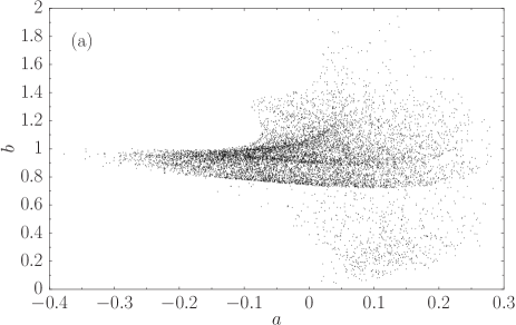
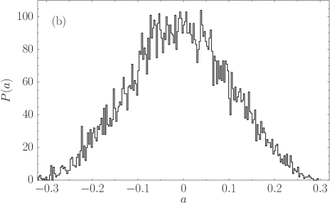
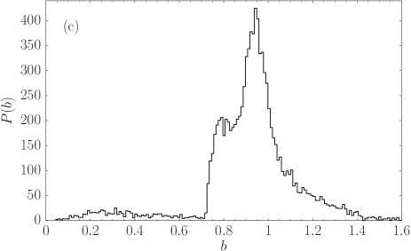
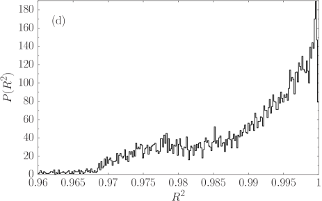
Figure 1: (a) Scatter plot of the fitting parameters $a$ and $b$ of Eq. (2) computed for each realization of the interacting two-level bosons ensemble for $k=2$ and $N=2000$. The frequency distributions of $a$, $b$, and $R^{2}$ are given in figures (b), (c), and (d), respectively.

Stochasticity is built into the Hamiltonian $\hat{H}_{k}^{(\beta)}$ at the level of the $k$–body matrix elements $v_{n,m}^{(\beta)}$. These matrix elements are assumed to be Gaussian distributed independent random variables, with zero mean and constant variance $v_{0}^{2}=1$. As in the case of RMT GMGW1998 , Dyson’s parameter $\beta$ distinguishes the ensembles according to its symmetry properties: $\beta=1$ corresponds to the case where time–reversal symmetry holds, and $\beta=2$ holds when time–reversal invariance is broken. The $k$–body interaction matrix $v^{(\beta)}$ is thus a member of the Gaussian Orthogonal Ensemble (GOE) for $\beta=1$ or of the Gaussian Unitary Ensemble (GUE) for $\beta=2$ GMGW1998 .

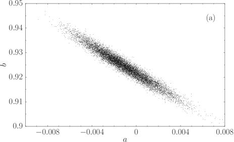
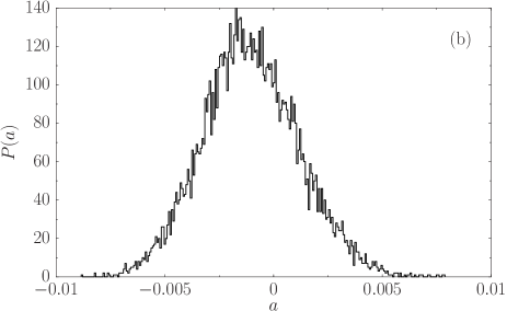
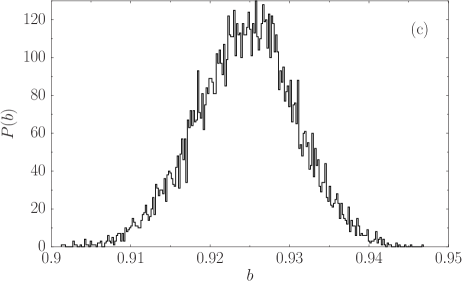
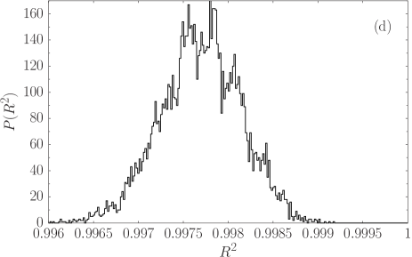
Figure 2: Same as Fig. 1 for $k=N$.

We note that the number of independent matrix elements of the $k$–body matrix is equal to $K_{\beta}(k)=\beta(k+1)(k+1+\delta_{\beta,1})/2$. Therefore, for $k\ll N$, which is physically the relevant case, the matrix elements of $\hat{H}_{k}^{(\beta)}$ are correlated, i.e., the number of independent random variables is much smaller than the number of independent matrix elements. In addition the matrix is sparse since many matrix elements are identically zero. The combinatorial factors ${\cal A}_{n,k}$ and ${\cal A}_{m,k}$ are introduced in the definition of the ensemble Eq. (1) in order to have for $k=N$ perfect identification, i.e., a one-to-one correspondence, with the canonical ensembles of RMT Asaga2001 ; BW2003 .

The numerical results presented below are related to the integrated level density, also referred to as the staircase function, of individual realizations of the ensemble (1). We take into account a large number of such realizations to achieve small statistical errors. For each member of the ensemble we construct the staircase function directly from the diagonalization of the Hamiltonian. The staircase function is defined as $\mathfrak{N}(E)=\Theta(E-\hat{H}_{k}^{(\beta)})=\sum_{i}\,\Theta(E-E_{i})$, where $E_{i}$ are the many-body eigenvalues of the specific realization of the Hamiltonian; $\Theta(x)$ is the Heaviside step function. By definition, the staircase function is a monotonic non-decreasing function of the energy. For later convenience we shall use the rank function $r(E)=N+1-\mathfrak{N}(E)$. We invert it numerically and express the energy $E$ in terms of the rank $r$; the function $E(r)$ is therefore a monotonic decreasing function of the rank $r$. For each member of the ensemble, the rank distribution $E(r)$ is fitted with the two-parameter distribution MartinezMekler :

$$f(r)=A\frac{(r_{\rm max}+1-r)^{b}}{r^{a}}.$$ (2)

Here, $A$ is the normalization constant of the distribution, $r_{\rm max}=N+1$ is the maximum value attained by the rank $r$, and the constants $a$ and $b$ are two fitting exponents. We refer to $f(r)$ as the discrete generalized beta distribution (DGBD).

We present now numerical results on the fitting exponents $a$ and $b$ of Eq. 2. These were obtained by considering $10000$ members of the $k$-body Gaussian Embedded Ensemble for two-level bosons, where we fixed $N=2000$ bosons and $\beta=1$; similar results were obtained for $\beta=2$. The best fit was determined by a log-log multiple linear regression; the quality of the fit is measured by the square correlation coefficient $R^{2}$, which must be close to $1$ for a reliable fit. We focus on the cases $k=2$ and $k=N$ since these are physically the most relevant. In Fig. 1 we present a scatter plot of the fitting parameters obtained for each individual member of the ensemble for $k=2$ and the frequency distributions of $a$, $b$, and $R^{2}$; Fig. 2 displays the corresponding results for $k=N$. Interestingly, these figures show that the distributions for $a$ and $b$ are much broader for $k=2$ than for $k=N$; the results on $R^{2}$ simply give confidence to the fitting procedure.

From the numerical results, we compute the average values of the fitting parameters. For $k=2$ we have $\bar{a}_{k=2}=-6.43\times 10^{-3}\pm 0.1094$ and $\bar{b}_{k=2}=0.922\pm 0.209$, where the assigned error corresponds to the standard deviation of the sample. Likewise, for $k=N$ we obtain $\bar{a}_{k=N}=-8.92\times 10^{-4}\pm 2.15\times 10^{-3}$ and $\bar{b}_{k=N}=0.924\pm 6.17\times 10^{-3}$. In both cases, $\bar{a}$ is slightly negative and very close to zero, and $\bar{b}<1$. We shall show in Section III that the fact that $\bar{a}\simeq 0$ and $\bar{b}\lesssim 1$ indicates that interactions mimic FES, i.e., interacting particles are equivalent to non-interacting Haldane quasi-particles with respect to the rank distribution.

III Rank distributions for fractional exclusion statistics

The combinatorial formula for the number of many–body states $W_{g}$ of $N$ identical particles following FES and occupying a group of $p$ states is given by (cf. page 147 of Muirhead1965 )

$$W_{g}=\frac{[p+(N-1)(1-g)]!}{N!\,[p-gN-(1-g)]!}.$$ (3)

This expression reproduces for $g=0$ the well-known expression for bosons, $W_{\rm B}=[p+N-1]!/[N!\,(p-1)!]$, and for $g=1$ that of fermions $W_{\rm F}=p!/[N!\,(p-N)!]$. Note that Eq. (3) can be rewritten as

$$W_{g}=\frac{[p^{\prime}+N-1]!}{N!\,[p^{\prime}-1]!},$$ (4)

with

$$p^{\prime}=p-g(N-1).$$ (5)

One has therefore $N$ identical bosons occupying an effective group of $p^{\prime}$ single-particle states. Note that $p^{\prime}$ could be formally negative. This gives the possibility of an interesting connection with the famous Regge trajectories used in high-energy physics Muirhead1965 .

In order to compare the rank distribution of $N$ particles obeying FES with those obtained in Section II for bosons, we shall group the $p^{\prime}$ single-particle levels filled by $N$ Haldane particles into two levels with energies $\epsilon_{0}=0$ and $\epsilon_{1}>\epsilon_{0}$, with $p^{\prime}=p_{0}^{\prime}+p_{1}^{\prime}$. If $p_{0}^{\prime}=1$, the number of (non-interacting Haldane particles) microstates with energy $E=n_{1}\epsilon_{1}$ is given by

$$\omega(n1=E/\epsilon_{1})=\frac{(n_{1}+p^{\prime}_{1}-1)!}{n_{1}!\,(p^{\prime}_{1}-1)!}\,.$$ (6)

The rank distribution with respect to the energy is then

$$r(E)=\sum_{\nu=E/\epsilon_{1}}^{N}\omega(\nu),$$ (7)

which for $p^{\prime}_{0}=1$ yields

$$r(E) = \sum_{\nu=0}^{N}\omega(\nu)-\sum_{\nu=0}^{E/\epsilon_{1}}\omega(\nu)$$ (8)

$$= \frac{(N+p_{1})!}{N!\,p_{1}!}-\frac{(E-\epsilon_{1}+p_{1})!}{(E-\epsilon_{1}-1)!\,p_{1}!}\,.$$

Taking the continuum limit of $E$ and using Stirling formula, we obtain

$$E\simeq(N^{p^{\prime}_{1}}-p^{\prime}_{1}!r)^{1/p^{\prime}_{1}}\,.$$ (9)

For particles obeying FES the effective number of states $p^{\prime}_{1}$ can be positive or negative, as we have remarked in connection with Eq. (5). If $p^{\prime}_{1}>0$ and $N$ is large, we have

$$\frac{E}{(p^{\prime}_{1}!)^{1/p^{\prime}_{1}}}=({\cal N}-r)^{1/p^{\prime}_{1}}\,,$$ (10)

with ${\cal N}=N^{p^{\prime}_{1}}/p^{\prime}_{1}!$, which is a discrete generalized beta distribution with $a=0$ and $b=1/p^{\prime}_{1}$, as seen from direct comparison with $f(r)$ in Eq. (2). On the other hand, if $p^{\prime}_{1}<0$ and $N$ is large, we have a rank distribution of the form

$$[(-p^{\prime}_{1})!r]^{-1/p^{\prime}_{1}}\,,$$ (11)

which corresponds to the values $a=1/|p^{\prime}_{1}|$ and $b=0$ of the DGBD. In order to have $(-p^{\prime}_{1})!$ real, $p^{\prime}_{1}$ must satisfy $-2s-1<p^{\prime}_{1}<-2s$, with $s$ a positive integer.

IV Discussion

We have given numerical evidence to show that the $k$-body embedded random matrix ensemble for bosons leads to an integrated level density which corresponds to a discrete generalized beta distribution. We have defined the ensemble for $N$ bosons interacting through a $k$-body force distributed in two single-particle levels. When $k=N$ the GOE is obtained by construction, and the two-body random ensemble French1970 for bosons corresponds to $k=2$, a more physical case.

The discrete generalized beta distribution fits rather well the statistical regularities in many instances: in particular, for the rank-citation profile of scientists Peterson . This distribution is present in systems whose output depends on the restricted difference of statistical variables Beltran . Examples of applicability are neuron dynamics (excitation and inhibition) and ecological community evolution (birth and death).

We then considered a set of independent Haldane quasiparticles, which obey fractional exclusion statistics, distributed in the same two-level system. It is shown that DGBD is also obtained. With respect to this distribution, at least, the above results indicate that the interaction among the particles makes the system equivalent to a set of quasiparticles obeying FES.

- (1) F. D. M. Haldane, Phys. Rev. Lett. 67, 937 (1991).
- (2) F. Calogero, J. Math. Phys. 10, 2191 (1969); F. Calogero, J. Math. Phys. 12, 419 (1971).
- (3) B. Sutherland, J. Math. Phys. 12, 246 (1971); B. Sutherland, Phys. Rev. A 4, 2019 (1971).
- (4) F. D. M. Haldane, J. Phys. C 14, 2585 (1981); J. L. Bagger, D. Nemeschansky, N. Seiberg and S. Yankielowicz, Nucl. Phys. B 289, 53 (1987), and references therein.
- (5) M. V. N. Murthy and R. Shankar, Phys. Rev. Lett. 72, 3629 (1994); M. V. N. Murthy and R. Shankar, Phys. Rev. Lett. 73, 3331 (1994); A.P. Polychronakos, Nucl. Phys. B 324, 597 (1989).
- (6) F. D. M. Haldane, Phys. Rev. Lett. 60, 635 (1988); B. S. Shastry, Phys. Rev. Lett. 60, 639 (1988); F. D. M. Haldane, Z. N. C. Ha, J. C. Talstra, D. Bernard and V. Pasquier, Phys. Rev. Lett. 69, 2021 (1992).
- (7) S. B. Isakov, Phys. Rev. Lett. 73, 2150 (1994); Int J Mod. Phys A 9, 2563 (1994); Mod. Phys. Lett. B 8, 319 (1994).
- (8) A. Khare, Fractional statistics and quantum theory. 2nd edition, World Scientific, Singapore, 2005
- (9) K. Iguchi and B. Sutherland, Phys. Rev. Lett. 85, 2781 (2000).
- (10) D. V. Anghel, Phys. Lett. A 372, 5745 (2008).
- (11) H. J. Lipkin, N. Meshkov and A. J. Glick, Nucl. Phys. 62, 188 (1965).
- (12) G.J. Milburn, J. Corney, E.M. Wright and D.F. Walls, Phys. Rev. A 55, 4318 (1997).
- (13) F. Iachello and A. Arima, The Interacting Boson Model, Cambridge University Press, Cambridge 1987.
- (14) T. Asaga, L. Benet, T. Rupp and H. A. Weidenmüller, Eurphys. Lett. 56, 340 (2001); T. Asaga, L. Benet, T. Rupp and H. A. Weidenmüller, Ann. Phys. (N.Y.) 298, 229 (2002).
- (15) L. Benet and H. A. Weidenmüller, J. Phys. A 36, 3569 (2003).
- (16) T. A. Brody, J. Flores, J. B. French, P. A. Mello, A. Pandey, and S. S. M. Wong, Rev. Mod. Phys. 53, 385 (1981).
- (17) T. Guhr, A. Mueller-Gröling and H. A. Weidenmüller, Phys. Rep. 299, 189 (1998).
- (18) G. Martínez-Mekler, et al., PLoS ONE 4, e4791 (2009).
- (19) T. Regge, Il Nuovo Cimento 14, 951 (1959).
- (20) S. Hernández-Quiroz and L. Benet, Phys. Rev. E. 81, 036218 (2010).
- (21) H. Muirhead, The physics of elementary particles, Pergamon Press (1965).
- (22) J.B. French and S. S. M. Wong, Phys. Lett. 33B, 449 (1970); O. Bohigas and J. Flores, Phys. Lett. 34B, 261 (1971).
- (23) A. M. Peterson, H. E. Stanley, and S. Succi, Scientific Reports, 1, 181, (2011)
- (24) M. Beltrán del Rio, G. Cocho, and R. Mansilla. Physica A, 390, 154, (2011)