Game Dynamics for Players
with Social and Material Preferences

Abstract

We consider the dynamics, existence and stability of the equilibrium states for large populations of individuals who can play various types of non–cooperative games. The players imitate the most attractive strategies, and the choice is motivated not only by the material payoffs of the strategies, but also by their popularity in the population. The parameter which determines the weights of both factors in the equilibrium states has the same analytical form for all types of considered games, and is identified with the sensitivity to reinforcements parameter in the Hernstein’s Matching Law. We prove theorems of existence and uniqueness, and discuss examples of multiple locally stable polymorphic equilibria for the considered types of games.

I Introduction

In the evolutionary game theory the theoretical approach to model the dynamics of populations is based on the proportional fitness rule. If the random matching and imitation of the individuals with highest payoffs are assumed, the equations which govern the evolution of such populations are the celebrated replicator equations, cf. e.g. Veg ; Gin1 ; Szabo ; McE ; HofSig ; Weibull , and references cited therein.

However, in general the individuals can be oriented not only toward imitating the highest payoff strategies, but they can also take into account other, "noneconomic" factors, in particular popularity of strategies in the population. The idea of combining together the bias towards imitating the strategies of the most payoff-successful agents and the strategies of the majority is not new, cf. for example Hen , where the ideas of imitating the successful, and copying the majority (the conformist transmission), are put together to stabilize the cooperation in populations of individuals, see also Han for another argument that noneconomic factors influence human’s behavior.

We consider a theory of evolution of social systems, that generalizes the standard proportional fitness rule of the evolutionary game theory. The biological fitness of a behavior, strategy, measured by its payoff from interactions, is replaced by more general function, the attractiveness of the behavior. The attractiveness of the strategy is assumed to depend not only on its payoff, but also on its actual popularity (fraction) in the population. The parameters of the attractiveness function describe different psychological characters of the members of the population. We consider the model based on the generalized Cobb–Douglas utility function, cf. Cob , Pla1 , Pla2 . We find a parameter that describes different personality profiles of the players, and that can be identified with the sensitivity to reinforcement in the Matching Law of mathematical psychology Her . In our setting it determines stability of polymorphic equilibria in all considered classes of games. We note that such equilibria for games with two strategies played in infinite populations were found for example in the aspiration–based models, cf. for example Pal ; Pla3 , in general multi-person games, cf. Gok , in the models of social dilemmas with synergy and discounting, cf. Hau3 , in the Stag-Hunt multi-person games, cf. for example Pac , in the multi-person Snowdrift game, cf. for example Sou and references cited therein.

We prove theorems of the existence of polymorphic equilibria, and identify sufficient conditions for their uniqueness for particular classes of the considered games. We also find examples of the existence of more than one (locally) stable polymorphism.

In the next section we formulate the general model and discuss its basic properties. In section III we briefly remind, for the convenience of the reader, an existence and uniqueness theorem for a general class of two-person symmetric games with two strategies, played in populations with social and material preferences, proved in Pla2 . We also provide examples of multiple stable internal equilibria for two-person symmetric games with three strategies. In section IV we discuss polymorphic equilibria for two-person asymmetric games with two strategies, and in section V we consider the multi–person games, in particular the Public Good game. In section VI we conclude and discuss some open problems.

II Model

We consider an infinite homogeneous population of individuals who interact through a random matching, playing at each instant of time a two–person or a multi–person non–cooperative game. The players have a finite number $K$ of behavioral types (strategies). Let $N_{i}(t)$ denotes the number of individuals playing the strategy $i,\$ $N=N_{1}+N_{2}+...N_{K}$–the fixed size of the system, $p_{i}=N_{i}/N\$–the frequency, or popularity of behavior $i$ for $i=1,2,...,K$.

The players who play a strategy $i$ review their strategy according to the Poisson process with the arrival rate $r_{i}$. We model the corresponding stochastic processes as a deterministic flow. The balance conservation equations read, cf. e.g. Weibull , section 4.4:

$$\dot{p}_{i}(t)=\sum_{j\neq i}[p_{j}r_{j}p_{j}^{i}-p_{i}r_{i}p_{i}^{j}],\ \ \ i=1,...K,$$ (1)

where $p_{j}^{i}$ is the probability that the agent playing the $j$ strategy will switch to the $i$ strategy.

We assume that $p_{j}^{i}$ is proportional to the attractiveness $u_{i}$ of the strategy $i$:

$$p_{j}^{i}=cu_{i}.$$ (2)

In general the attractiveness of a strategy can be a complicated function of various factors, describing the state of the system and the characteristics of the players. Many social and biological interactions are based on imitation processes, where individuals adopt more successful and more popular strategies with larger probability than less successful and less popular ones. We choose for the attractiveness of the strategy $i$ the generalized Cobb-Douglas utility function, cf. Cob ; Pla1 ; Pla2 :

$$u_{i}(t)=p_{i}^{1-\alpha}\nu_{i}^{1-\beta},\ \ \ i=1,...,K,$$ (3)

with $(\alpha,\beta)\in[0,1]\times[0,1].$ The formula (3) states that the attractiveness of a strategy depends not only on the payoff of the strategy, but also on its actual popularity in the population. The parameters $\alpha,\ \beta$ determine the responsiveness of the function $u_{i}$ to changes of the current popularity and of the mean payoff of the action $i$. They define different social and material preferences of the individuals, in other words their different personality profiles.

More attractive strategies ought to have an evolutionary advantage in the considered social systems. Note that the attractiveness of the strategy $i$ is increasing and concave function of both arguments, i.e. of the mean payoff $\nu_{i}$ and of the popularity $p_{i}$ in the population. In particular when the attractiveness reaches a higher level, the changes are slower. The attractiveness of the strategy becomes zero if its mean payoff or its popularity in the population is zero. In the Appendix, p. A we define and characterize the ideal types of the personality profiles for $\alpha,\beta\in\{0,1\}$, and characterize their basic properties, cf. Pla1 ; Pla2 . All other values of the parameters $\alpha,\beta$ describe intermediate personality profiles. We show below that the combination of these parameters

$$s=\frac{1-\beta}{\alpha},$$ (4)

plays a crucial role in determining the polymorphic equlibria and their stability, and can be identified with the sensitivity parameter which links the relative rates of reinforcements and responses in the Hernstein’s Matching Law Her .

As postulated in (2), the strategies with higher attractivenesses have larger probability to be imitated. Assuming that the arrival rates $r_{j}$ are constants, and rescaling the time we obtain the system of equations which has the formal structure analogous to the replicator equations:

$$\dot{p}_{i}(t)=u(\frac{u_{i}}{u}-p_{i}),\ \ \ \ \ u:=\sum_{j=1}^{K}u_{j},\ \ i=1,2,...,K.$$ (5)

Thus, the fraction $p_{i}$ of strategy $i$ increases if its normalized attractiveness $\frac{u_{i}}{u}\in[0,1]$ is bigger than the actual fraction of the strategy $i$, and decreases if it is smaller. In particular, for $\alpha=\beta=0$, corresponding to Homo Afectualis (cf. the Appendix, p. A) the evolution equations (5) are identical to the replicator equations of the evolutionary game theory.

All critical points of the dynamics (5) are obtained as solutions of the system of $K-1$ algebraic equations

$$\frac{u_{1}}{p_{1}}=\frac{u_{2}}{p_{2}}=...=\frac{u_{K}}{p_{K}}.$$ (6)

which, after substituting (3) is equivalent to

$$\frac{p_{i}}{p_{1}}=\left(\frac{\nu_{i}}{\nu_{1}}\right)^{s},\quad i=1,...,K,$$

where $\nu_{i}\$ is the mean payoff of strategy $i$. In particular the stability properties of the solutions of eqs. (6) depend on the combination $s$ of the parameters $\alpha,\beta$, which characterize the personality profile of the players, rather than separately on each of them. The sensitivity parameter $s$ plays an important role in the matching law in the operant response theory of the mathematical psychology, in particular as a measure of the degree to which, in equilibrium, the response ratio changes when the reinforcement ratio is modified, cf. for example Her ; Pla1 ; Pla2 , and references cited therein.

III Equilibria for Two-Person Symmetric Games

In this section we consider populations which play symmetric 2-person games. For a convenience of the reader we first remind the results for the case of two strategies, proved in Pla2 .

III.1 2-Person Games with 2 Strategies

For the symmetric 2-person games with two strategies (denoted 1,2), with the payoff matrix

$$\begin{array}[]{r|cc}&1&2\\ \cline{1-3}\cr\hline\cr 1&a&b\\ 2&c&d\end{array}$$ (7)

where $a,b,c,d$ are arbitrary positive numbers, we obtain the full characterization of the equilibria. With the normalization condition $p_{1}+p_{2}=1$ eq. (5) reduces to the evolution equation

$$\dot{p}_{1}=(1-p_{1})^{1-\alpha}p_{1}^{1-\alpha}[\nu_{1}^{1-\beta}(1-p_{1})^{\alpha}-\nu_{2}^{1-\beta}p_{1}^{\alpha}],$$ (8)

with $\nu_{1}=(a-b)p_{1}+S,\ \ \nu_{2}=(c-d)p_{1}+d.$ For each personality profile $(\alpha,\beta)\in[0,1]\times[0,1]$ there exist two pure equilibria of (5): $p_{1}=0$ and $p_{1}=1$ [for $\alpha=1$ we put $u_{i}(p_{i}=0)=0,\ i=1,2$]. The equilibria of eq. (5) in which each strategy has a non zero frequency will be called Mixed Equilibria, and denoted ME. Each ME corresponds to a fixed point of eq. (8). For the symmetric 2-person games the following theorem is true:

Theorem 1.

  

For the payoff matrix (7) with positive entries:

I. For each $0\leq s<\infty$ there exists at least one ME – the fixed point of the evolution equation (8).

II. Denote $B:=(1-s)\frac{d}{c}+(1+s)\frac{b}{a},\ \ \Delta:=B^{2}-4\frac{bd}{ac}.$ If 1. $\Delta\leq 0,$ or 2. $B\geq 0$, or 3. $bc\geq ad$, then ME is unique.

III. For each $0\leq s<\infty$ there exist at most three ME.

IV. There exist three ME iff $\Delta>0,\ \ B<0,\ \mbox{and}\ U(z_{1})U(z_{2})<0,$ where $z_{1,2}:=[-B\mp\sqrt{\Delta}]/2,$ and $U(z):=lnz+s\ ln{\frac{cz+d}{az+b}},\ \ z>0.$

V. If a ME is unique, then it is globally stable in $(0,1)$ under the considered dynamics. If there are three ME, then the middle one is (locally) instable, the other two stable.

The statement I implies that the dependence of the attractiveness of a strategy on its popularity implies the existence of at least one ME for all symmetric two-person games with positive payoffs, including all types of the social dilemma games. In particular this "solves the dilemma" of the Prisoner’s Dilemma population game. The statement II.2 implies that for $s\leq 1$ the cooperation level is unique, and does not depend on the initial distribution of strategies. For the proof, interpretations and applications to various types of 2-person games the reader is referred to Pla2 .

III.2 2-Person Symmetric Games with 3 Strategies

III.2.1 General results

2-person symmetric games with 3 strategies play important role in the population game theory. First we formulate the general setting in the frame of populations with complex personality profiles, then we discuss particular types of such games.

The general symmetric 2-person game with 3 strategies, denoted 1, 2, 3, has the payoff matrix

$$\begin{array}[]{r|ccc}&1&2&3\\ \hline\cr 1&a_{11}&a_{12}&a_{13}\\ 2&a_{21}&a_{22}&a_{23}\\ 3&a_{31}&a_{32}&a_{33}\end{array}$$ (9)

where we assume $a_{ij}>0\ \forall i,j\in\{1,2,3\}.$ The mean payoffs of strategies $1,2,3$ are defined as

$$\nu_{i}(t) =\sum_{j=1}^{3}a_{ij}p_{j}(t),\quad i=1,2,3,$$ (10)

with $p_{3}=1-p_{1}-p_{2}$. The dynamical system (5) has the form

$$\dot{p}_{1} =p_{1}^{1-\alpha}(1-p_{1})\nu_{1}^{1-\beta}-p_{1}[p_{2}^{1-\alpha}\nu_{2}^{1-\beta}+(p_{3})^{1-\alpha}\nu_{3}^{1-\beta}],$$ (11)

$$\dot{p}_{2} =p_{2}^{1-\alpha}(1-p_{2})\nu_{2}^{1-\beta}-p_{2}[p_{1}^{1-\alpha}\nu_{1}^{1-\beta}+(p_{3})^{1-\alpha}\nu_{3}^{1-\beta}].$$ (12)

For the 3-strategy games we define mixed equilibria (ME) of (11) as the critical points of the above dynamical system with all nonzero coordinates $p_{i},\ i=1,2,3$. We shall alternatively use the term polymorphic equilibria. With notation

$$x:=\frac{p_{2}}{p_{1}},\quad y:=\frac{p_{3}}{p_{1}}$$ (13)

the equations for ME can be written, using (3), (6), (10), in the form

$$x =\left(\frac{a_{21}+a_{22}x+a_{23}y}{a_{11}+a_{12}x+a_{13}y}\right)^{s},$$ (14)

$$y =\left(\frac{a_{31}+a_{32}x+a_{33}y}{a_{11}+a_{12}x+a_{13}y}\right)^{s}.$$ (15)

The frequencies of the strategies in ME are obtained from the reverse formulas:

$$p_{1}=\frac{1}{1+x+y},\ \ p_{2}=p_{1}x,\ \ p_{3}=p_{1}y.$$ (16)

In general the number of ME and their stability depend on the payoff matrix and on the sensitivity parameter $s$.

One of the most celebrated 3-strategy games is the Rock-Paper-Scissor (RPS) game, cf. for example HofSig ; Weibull . The population of players with complex personality profiles, playing the RSP game has been investigated in Pla4 . In particular, in the "standard" RPS game the critical point $(\frac{1}{3},\frac{1}{3},\frac{1}{3})$ is asymptotically stable for all $\alpha,\beta\in(0,1]$. For other properties of the solutions, in particular the existence of limit cycles, the Hopf and the Boutin–like bifurcations, the reader is referred to Pla4 .

Below we analyze other important classes of 3–strategy symmetric games, in particular the coordination games, for which there exist multiple stable polymorphic equilibria, and the iterated Prisoner’s Dilemma game with three strategies AllD, AllC, TFT, with unique stable ME.

III.2.2 Coordination Game

We consider the coordination game with 3 strategies and the payoff matrix

$$\begin{array}[]{r|ccc}&1&2&3\\ \hline\cr 1&2&1&1\\ 2&1&3&1\\ 3&1&1&3\end{array}$$ (17)

We demonstrate the existence of three ME for $s=3$. For $s=1$ the system (14), (15) can be solved explicitly. The unique nonnegative solution is $x=y=\frac{1}{2}(1+\sqrt{3}),$ which, according to (16), gives the equilibrium state $(p_{1},p_{2},p_{3})$ with the frequencies $p_{1}=2-\sqrt{3},\ \ p_{2}=p_{3}=\frac{1}{2}(\sqrt{3}-1).$

For $s=2$ the system (14), (15) is of the third order. In order to obtain analytical solution we subtract (15) from (14), and obtain the equation

$$(x-y)(2+x+y)^{2}=4(x-y)(1+2x+2y).$$ (18)

It can be easily shown that (18) has positive solution only if $y=x$, in which case the solution of the system (14), (15) is the pair $(x_{0},x_{0})$, where $x_{0}\cong 2.45$ is the unique positive root of the polynomial

$$F(x)=4x^{3}-8x^{2}-4x-1.$$ (19)

The corresponding unique equilibrium state reads $(p_{1},p_{2},p_{3})\cong(0.17,0.415,0.415).$ When we farther increase the value of the sensitivity parameter $s$ the uniqueness is lost. In Figure 1 we show time evolution of frequencies ($p_{1},p_{2},p_{3}$) for two values of the sensitivity parameter $s$ for particular initial data, symmetric with respect to $p_{10}$ (i.e. for $p_{20}=p_{30}$). For $s=2.15$ the equilibrium is unique (not shown). For a value $s\geq s_{0}\in(2.15,2.30)$ there emerge multiple equilibria. For $s=3$ (left diagram), and $s=3.75$ (right diagram) there are three ME, two of them stable, one unstable. In each diagram the frequencies reach asymptotically one of the stable ME. Note the influence of the unstable equilibrium in the early stage of the evolution. First the trajectory approaches the unstable symmetric ME $(p_{1},p_{2},p_{3})\cong(0.14,0.43,0.43)$, then it tends to the locally stable equilibrium: $(p_{1},p_{2},p_{3})\cong(0.126,0.225,0.649)$. The other "symmetric" locally stable ME is $(p_{1},p_{2},p_{3})\cong(0.126,0.649,0.225)$. The amount of time the trajectory stays in a neighborhood of the unstable equilibrium depends on the sensitivity parameter $s$, and on the personality profile parameters $\alpha,\beta$. For $s=3.75$ both locally stable ME tend to the relevant vortexes of the game simplex, cf. the right diagram in Figure 1.

We explain the emergence of the multiple equilibria for $s=3$. First we look for the symmetric solution $p_{2}=p_{3}$, i.e. $x=y$. The system (14), (15) reduces to one equation

$$8x^{4}-40x^{3}-24x^{2}-4x-1=0.$$ (20)

The unique positive root of the polynomial in (20) is $x\cong 5.556$. The corresponding equilibrium reads $(p_{1},p_{2},p_{3})\cong(0.082,0.459,0.459)$. There are two other, symmetric ME. The first zero gives the ME: $(p_{1},p_{2},p_{3})\cong(0.047,0.057,0.896)$. As expected from the symmetry of the second and third strategy, the second zero gives the "symmetric" ME: $(p_{1},p_{2},p_{3})\cong(0.047,0.896,0.057)$. There are also four "partially mixed" equilibria: two on the edge $p_{1}=0$, and one on each other edges, in the neighborhood of the corners 2 and 3, i.e. near $p_{2}=1$ and $p_{3}=1$. For increasing values of the sensitivity parameter $s$ the stable equilibria approach the relevant edges of the game simplex.

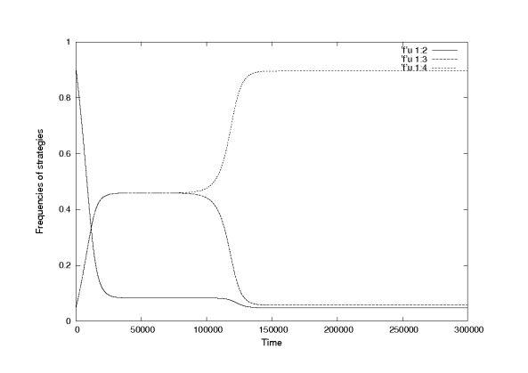
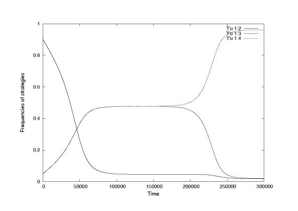
Figure 1: Time evolution of frequencies $p_{1},p_{2},p_{3}$ for the coordination game (17). Left: $s=3$, right: $s=3.75$.

In the Appendix, p. B we prove the existence and uniqueness theorem for another class of the asymmetric coordination games, in which both players are better off if they play different strategies (anti–coordination games).

III.2.3 Repeated Prisoner’s Dilemma Game

Another interesting example of three–strategy games is the 2–person,  3–strategy finitely repeated Prisoner’s Dilemma Game with the payoff matrix

$$\begin{array}[]{r|ccc}&AllC&AllD&TFT\\ \hline\cr AllC&Rm&Sm&Rm\\ AllD&Tm&Pm&T+P(m-1)\\ TFT&Rm&S+P(m-1)&Rm\end{array}$$ (21)

where $T>R>P\geq S$ are the payoffs in the one-shot PD game, AllC (AllD) is the strategy: play always C (play always D), TFT is the strategy Tit for Tat, and $m$ is the number of rounds.

In the classical replicator dynamics, with the payoff from TFT additionally reduced by a small value (the cost of playing TFT) it has been shown in FudNow , that the population evolves through the cycles of cooperation and defection.

For the general matrix (21) we checked numerically the existence and uniqueness of ME for for wide ranges of the payoffs $T>R>P\geq S$ and of the parameters $m,s$. Moreover, the share (sum of the frequencies) of the cooperative strategies AllC and TFT decreases for increasing ratio $\frac{T}{R}$ and increasing number of rounds, whereas for increasing $m$ it increases, in agreement with intuition.

For the Weak Prisoner’s Dilemma ($P=S=0$) we prove

Corollary 2.

  

There exists an unique ME: $(p_{1},p_{2},p_{3})=(\frac{1}{2+a},\frac{a}{2+a},\frac{1}{2+a})$, where $a=[\frac{T(m+1)}{2mR}]^{s}$, of the game (21) with $P=S=0$, for all nonnegative sensitivity parameters $s$.

Proof.

Eq. (15) for the ME gives $y=1$. Eq. (14) gives $a=[\frac{T(m+1)}{2m}]^{s}$, and the result follows from (16). ∎

Note that for the increasing ratio $\frac{T}{R}$ the shares of the AllC and TFT players in ME decrease, whereas for increasing $m$ they increase, as in the case of the general payoff matrix (21).

IV 2-Person Asymmetric Games

IV.1 General Results

In this section we consider 2-person games played between members of two populations with (in general) different personality profiles. The members of both populations choose between two strategies $A$ and $B$. The payoff matrix reads

$$\left[\begin{array}[]{cc}(a_{1},a_{2})&(b_{1},b_{2})\\ (c_{1},c_{2})&(d_{1},d_{2})\end{array}\right],$$ (22)

with nonnegative entries. In general the strategies in both populations may be different meanings. For simplicity we do not use different notation for the relevant pairs of strategies. The row players belong to the population $i=1$, and the column ones to  $i=2$. We denote $x_{i},\ i=1,2,$ the fraction of population $i$ which plays strategy $A$.

Let $(\alpha_{i},\beta_{i})$ describe the personality profile of the individuals of population $i,\ i=1.2$. The members of each population may put different weights to the payoffs and popularities of the available strategies in the imitation process.

We define $u_{j}^{i}$–the attractiveness of strategy $j\in\{A,B\}$ in population $i\in\{1,2\}$:

$$u_{A}^{i} = x_{i}^{1-\alpha_{i}}\nu_{Ai}^{1-\beta_{i}},$$ (23)

$$u_{B}^{i} = (1-x_{i})^{1-\alpha_{i}}\nu_{Bi}^{1-\beta_{i}},$$ (24)

where $\nu_{ji}$ is the mean payoff from strategy $j$ in population $i$:

$$\nu_{A1}=a_{1}x_{2}+b_{1}(1-x_{2}),\ \ \nu_{B1}=c_{1}x_{2}+d_{1}(1-x_{2}),\ \ \nu_{A2}=a_{2}x_{1}+c_{2}(1-x_{1}),\ \nu_{B2}=b_{2}x_{1}+d_{2}(1-x_{1}).$$

Thus, the attractiveness of each strategy of a population depends on two factors: the ”social” one, represented by the fraction, popularity of the strategy in the population, and the ”economic” one, represented by the mean payoff of this strategy in the considered population. Note that the social factor depends on the composition of the considered population, whereas the economic one depends on the composition of the second population. This can be interpreted in the following way: the members of each population determine their strategy choice observing popularity of the available strategies in their own population, and their payoffs from the interactions with the members of the other population.

The dynamics (5), written for asymmetric games, reads

$$\begin{array}[]{rcl}\dot{x}_{1}&=&(1-x_{1})x_{1}^{1-\alpha_{1}}\nu_{A1}^{1-\beta_{1}}-x_{1}(1-x_{1})^{1-\alpha_{1}}\nu_{B1}^{1-\beta_{1}},\\ \dot{x}_{2}&=&(1-x_{2})x_{2}^{1-\alpha_{2}}\nu_{A2}^{1-\beta_{2}}-x_{2}(1-x_{2})^{1-\alpha_{2}}\nu_{B2}^{1-\beta_{2}}.\end{array}$$ (25)

Note that for $\alpha_{i}=\beta_{i}=0,i=1,2$ the system (25) reduces to the replicator dynamics for asymmetric games, cf. for example HofSig ; Weibull . The pairs of $(x_{1},x_{2})$: $(0,0),(0,1),(1,0),(1,1)$ are equilibria in pure strategies of (25). They correspond to the situations in which each population plays only one of two available strategies. We are looking for the mixed equilibria (ME) in which both strategies have nonzero frequencies for each population.

With the substitution $z_{i}=\frac{x_{i}}{1-x_{i}},\ i=1,2$ the system reads

$$\begin{array}[]{rcl}\dot{z_{1}}&=&z_{1}^{1-\alpha_{1}}(1+z_{1})^{\alpha_{1}}\nu_{A1}^{1-\beta_{1}}-z_{1}(1+z_{1})^{\alpha_{1}}\nu_{B1}^{1-\beta_{1}},\\[5.69054pt] \dot{z_{2}}&=&z_{2}^{1-\alpha_{2}}(1+z_{2})^{\alpha_{2}}\nu_{A2}^{1-\beta_{2}}-z_{2}(1+z_{2})^{\alpha_{2}}\nu_{B2}^{1-\beta_{2}}.\end{array}$$ (26)

From (26) we obtain the algebraic equations for ME:

$$\begin{array}[]{rcl}\bar{z}_{1}=\left(\frac{a_{1}\bar{z}_{2}+b_{1}}{c_{1}\bar{z}_{2}+d_{1}}\right)^{s_{1}},\quad\bar{z}_{2}=\left(\frac{a_{2}\bar{z}_{1}+b_{2}}{c_{2}\bar{z}_{1}+d_{2}}\right)^{s_{2}},\end{array}$$ (27)

where

$$s_{i}=\frac{1-\beta_{i}}{\alpha_{i}},\quad i=1,2$$ (28)

denotes sensitivity of players in population $i$. Thus, for the asymmetric 2-person games the ME are determined by relevant combinations of parameters $s_{1},s_{2}$ which describe the personalities of players respectively in the first and the in the second population. In the next subsections we show the existence of ME for typical asymmetric games. Here we prove that, contrary to the replicator equations for asymmetric 2-person games, the solutions can not be periodic.

Theorem 3.

The system (26) does not have periodic solutions.

Proof.

We define the function $\phi(z_{1},z_{2})=[z_{1}(1+z_{1})^{\alpha_{1}}z_{2}(1+z_{2})^{\alpha_{2}}]^{-1}$, and note that

$$\frac{\partial(\phi\dot{z}_{1})}{\partial z_{1}}+\frac{\partial(\phi\dot{z}_{2})}{\partial z_{2}}=-\frac{\alpha_{1}z_{1}^{-(\alpha_{1}+1)}\nu_{A1}^{1-\beta_{1}}}{z_{2}(1+z_{2})^{\alpha_{2}}}-\frac{\alpha_{2}z_{2}^{-(\alpha_{2}+1)}\nu_{A2}^{1-\beta_{2}}}{z_{1}(1+z_{1})^{\alpha_{1}}}<0,$$

for $z_{1},z_{2}>0$. Applying the criterion  Dulac–Bendixson we obtain the thesis. ∎

IV.2 Asymmetric coordination games

IV.2.1 Pure coordination games

We consider the model defined in the previous section for the asymmetric coordination games with the payoff matrix

$$\left[\begin{array}[]{cc}(a_{1},a_{2})&(0,0)\\ (0,0)&(d_{1},d_{2})\end{array}\right],$$ (29)

and $a_{i}\neq 0,\ d_{i}\neq 0,\ i=1,2,$ played between two populations with different personality profiles. Such games will be called pure (asymmetric) coordination games. We can for example think about two populations of different sexes, $i=1$ and $i=2$ denote respectively men’s and woman’s populations. For $a_{1}>d_{1},\ a_{2}<d_{2}$ this corresponds to the well known Battle of Sexes game. Players from each population evaluate the available strategies according to their attractiveness, calculated for each of two populations $i=1,2$ with the personality profiles ($\alpha_{i},\beta_{i}$), according to formulas (23). With notation (28) we prove the following theorem

Theorem 4.

  

If $s_{1}s_{2}\neq 1$ then there exists a unique ME of the dynamics (26) for the populations with the payoff matrices (29):

$$\bar{z}_{1}=\left(\frac{a_{1}a_{2}^{s_{2}}}{d_{1}d_{2}^{s_{2}}}\right)^{\frac{s_{1}}{1-s_{1}s_{2}}},\quad\bar{z}_{2}=\left(\frac{a_{1}^{s_{1}}a_{2}}{d_{1}^{s_{1}}d_{2}}\right)^{\frac{s_{2}}{1-s_{1}s_{2}}}.$$ (30)

The equilibrium (30) is locally asymptotically stable if $s_{1}s_{2}<1$, and unstable if $s_{1}s_{2}>1$.

If $s_{1}s_{2}=1$ then for $(a_{1}/b_{1})^{s_{1}}a_{2}^{s_{2}}\neq 1$ there are no ME, for $(a_{1}/b_{1})^{s_{1}}a_{2}^{s_{2}}=1$ there exists the family of ME $\bar{z}_{1}=c,\quad\bar{z}_{2}=c^{s_{1}}(a_{2}/b_{2})^{s_{2}}$, where $c$ is an arbitrary positive constant.

Proof: cf. the Appendix, p. C. Numerical simulations indicate that if the equilibrium (30) is locally stable then it attracts all investigated trajectories from the interior of the simplex of the game. We note that the replicator dynamics for the considered asymmetric games (which formally coresponds to infinite sensitivities in our dynamics, has an unique ME, which is Lapunov stable. In Appendix, p. D, we prove analogous existence and uniqueness theorem for another class of asymmetric games (anti–coordination games), in which the players are better off if they use different strategies.

IV.2.2 Coordination games with multiple ME

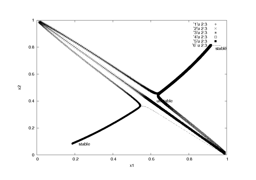
Figure 2: Examples of trajectories and critical points for the asymmetric coordination game (31): $a_{1}=d_{2}=3,a_{2}=d_{1}=2,b_{i}=c_{i}=1,i=1,2.$ All six displayed trajectories start from a neighborhood of the points $(0,1)$ or $(1,0)$.

In asymmetric coordination games the positivity of payoffs plays crucial role in the uniqueness problem, and in determining the polymorphic equilibria. In the pure coordination games considered above the ME is unique, whereas in general coordination games multiple stable polymorphic equilibria are possible. For example, the 2-person asymmetric game with the payoff matrix

$$\left[\begin{array}[]{cc}(3,2)&(1,1)\\ (1,1)&(2,3)\end{array}\right],$$ (31)

has, for $s_{1}=s_{2}=3$, three ME, corresponding to $(x_{1}\approx 0.92,x_{2}\approx 0.82)$, $(x_{1}=0.6,x_{2}=0.40)$, and $(x_{1}\approx 0.18,x_{2}\approx 0.08)$, as can be checked solving (27). Two equilibria are locally stable, one unstable, cf. Fig. 2.

V Multi-person Games

V.1 General results

In this section we consider multi-person one-shot symmetric games in which each of $N$ players chooses one of two actions: C or D, C stands for cooperation, D for defection. In order to obtain symmetric notation and formulas, we define $n:=N-1$, and from now on we consider the $n+1$–person games. This allows to define:

$$\left\{\begin{array}[]{cl}a_{k}:&\textrm{the payoff of player \ }C\textrm{, when k others play \ }C,\\ b_{k}:&\textrm{the payoff of player \ }D\textrm{, when k others play \ }D,\end{array}\right.$$

where $k\in\{0,\ \ldots,\ n\},$ and $a_{k},\ b_{k}\geq 0$.

Let $x$ denote the fraction of the population that plays $C$. The mean payoffs from both strategies are respectively

$$\nu_{C} = \sum_{k=0}^{n}{n\choose k}x^{k}(1-x)^{n-k}a_{k},$$

$$\nu_{D} = \sum_{k=0}^{n}{n\choose k}x^{k}(1-x)^{n-k}b_{k}.$$

The evolution equation reads

$$\dot{x}=(1-x)x^{1-\alpha}\nu_{A}^{1-\beta}-x(1-x)^{1-\alpha}\nu_{B}^{1-\beta},$$ (32)

Substituting $z=\frac{x}{1-x}$ we obtain

$$\dot{z}=f(z)\left(\left(\frac{W_{A}(z)}{W_{B}(z)}\right)^{1-\beta}-z^{\alpha}\right),$$ (33)

where $W_{A}(z)=\sum\limits_{k=0}^{n}{n\choose k}a_{k}z^{k}$, $W_{B}(z)=\sum\limits_{k=0}^{n}{n\choose k}b_{k}z^{k}$, and  $f(z)$ is a positive function which does not influence the equilibria and their stabilities but only the speed of the evolution.

Stationary points of the dynamics described by (33) can be obtained solving the equation

$$\bar{z}=\left(\frac{W_{A}(\bar{z})}{W_{B}(\bar{z})}\right)^{s},$$

where $s=\frac{1-\beta}{\alpha}$ is the previously defined sensitivity coefficient. We prove the following

Theorem 5.

  

The dynamics (32) of the symmetric $(n\!+\!1)$–person game has at most $2n+1$ mixed equilibria.

Proof.

We define the function $U(z)\colon\mathbb{R}_{+}\to\mathbb{R}_{+}$:

$$U(z)=s\ln{\frac{W_{A}(z)}{W_{B}(z)}}-\ln{z}.$$

Zeros of $U$ are stationary points of the considered dynamics, and $\operatorname{sgn}(U(z)|_{z_{0}})=\operatorname{sgn}(\dot{z}|_{z_{0}})$.

It is sufficient to show that $U(z)=0$ at at most $2n+1$ points in $(0,+\infty)$. To this end we calculate

$$U^{\prime}(z)=s\frac{W_{A}^{\prime}}{W_{A}}-s\frac{W_{B}^{\prime}}{W_{B}}-\frac{1}{z}=\frac{sW_{A}^{\prime}W_{B}z-sW_{B}^{\prime}W_{A}z-W_{A}W_{B}}{W_{A}W_{B}z}.$$

The polynomial $sW_{A}^{\prime}W_{B}z-sW_{B}^{\prime}W_{A}z-W_{A}W_{B}$ is at most of the order $2n$, therefore $U^{\prime}(z)$ has at most $2n$ zeros. Since between each two zeros of $U$ there has to be a zero of $U^{\prime}(z)$, the function $U(z)$ can have at most $2n+1$ zeros. ∎

Theorem 6.

  

For the (n+1)–person games with two strategies and with all payoffs positive there exists at least one mixed equilibrium.

Proof.

Due to continuity of the considered dynamics is enough to prove that both boundary equilibrium points corresponding to pore equilibria: $x=0,\ x=1$ are unstable. This will be proved in two lemmas below. ∎

Lemma 1.

Let $p=\min{\{i\colon a_{i}>0\}},\ r=\min{\{i\colon b_{i}>0\}}$. If

$$ps>rs+1,$$ or (34)

$$ps=rs+1 {n\choose p}a_{p}<{n\choose r}b_{r},$$ and (35)

then the point $x=0$ is asymptotically stable. If

$$ps<rs+1,$$ or

$$ps=rs+1 {n\choose p}a_{p}>{n\choose r}b_{r},$$ and

then the point $x=0$ is unstable.

Proof.

We note that

$$W_{A}(z) = {n\choose p}a_{p}z^{p}+O(z^{p}),$$

$$W_{B}(z) = {n\choose r}b_{r}z^{r}+O(z^{r}).$$

We obtain

$$\textrm{for the condition (\ref{war1a}):}\ \ \lim_{z\to 0}U(z) = \lim_{z\to 0}\ln\left(\frac{(W_{A}(z))^{s}}{(W_{B}(z))^{s}z}\right)=-\infty,$$

$$\textrm{for the condition (\ref{war1b}):}\ \ \lim_{z\to 0}U(z) = \ln\left(\frac{{n\choose p}a_{p}}{{n\choose r}b_{r}}\right)<0.$$

In our one dimensional system the stationary point $\bar{z}>0$ is asymptotically stable iff $\exists_{\varepsilon>0}\ \dot{z}|_{(\bar{z},\bar{z}+\varepsilon)}<0\land\dot{z}|_{(\bar{z}-\varepsilon,\bar{z})}>0$. The sufficient condition is $U^{\prime}(\bar{z})<0$. On the contrary, if $U^{\prime}(\bar{z})>0$, then the point $\bar{z}$ is unstable. Analogously, the sufficient condition for stability of $z=0$ reads: $\lim_{z\to 0}U(z)<0$. Since $\operatorname{sgn}(U(z_{0}))=\operatorname{sgn}(\dot{z}|_{z_{0}})$, then in the cases (34) and (35) we have $\dot{z}<0$ for a certain $\varepsilon_{z}>0$ and $z\in(0,\varepsilon_{z})$. From the equality $\dot{x}=\frac{\dot{z}}{(1+z)^{2}}$ it follows, that then for a certain $\varepsilon_{x}>0$ and  $x\in(0,\varepsilon_{x})$ we have $\dot{x}<0$.

The proof of the second part of Lemma 1 is analogous. ∎

Lemma 2.

Let $p^{\prime}=\max{\{i\colon a_{i}>0\}},\ r^{\prime}=\max{\{i\colon b_{i}>0\}}$. If

$$p^{\prime}s>r^{\prime}s+1,$$ or

$$p^{\prime}s=r^{\prime}s+1 {n\choose p^{\prime}}a_{p^{\prime}}>{n\choose r^{\prime}}b_{r^{\prime}},$$ and

then the point $x=1$ is asymptotically stable. If

$$p^{\prime}s<r^{\prime}s+1,$$ or

$$p^{\prime}s=r^{\prime}s+1 {n\choose p^{\prime}}a_{p^{\prime}}<{n\choose r^{\prime}}b_{r^{\prime}},$$ and

then the point $x=1$ is unstable.

Proof.

It is enough to apply Lemma 1 with the strategies interchanged. ∎

The above theorem guarantees the existence, however not uniqueness of the ME (we remind that for the 2-person symmetric games with positive payoffs the uniqueness has been proved for $s\leq 1$. Below we give an example of a 3-person game with positive payoffs and three ME for the sensitivity $s=1$.

Example

Let $a_{0}=5,\ a_{1}=a_{2}=1,\ b_{0}=1,\ b_{1}=\frac{2}{3},\ b_{2}=5\frac{1}{3}$. The corresponding payoff matrix reads:

$$\begin{array}[]{r|ccc}&11&12&22\\ \hline\cr 1&5&1&1\\ 2&1&\frac{2}{3}&5\frac{1}{3}\end{array}$$ (36)

Note that this game can be treated as a coordination game (the players are better off if they play the same strategies). The equation for ME reads:

$$z=\left[\frac{a_{0}z^{2}+a_{1}z+a_{2}}{b_{0}z^{2}+b_{1}z+b_{2}}\right]^{s},$$ (37)

which, for $s=1$ has three positive roots, resulting, after substitution $z=\frac{x}{1-x}$ in three ME: $x_{1}=\frac{1}{4},\ x_{2}=\frac{1}{2},\ ,x_{1}=\frac{3}{4}$. We checked that $x_{1}$ and $x_{3}$ are locally stable, and $x_{2}$ unstable.

V.2 Public Goods game

We apply the general results of the previous subsection to the important $(n+1)$–person game–the Public Goods (PG) game. In this game each of $(n+1)$ players receives an amount $g$, and chooses one of two actions: C: Contribute with $g$ into the common pool or D: Do not contribute. Let $k$ among $n+1$ players choose C. The amount $kg$ in the common pool is multiplied by $r,\ \ n+1>r>1$, and distributed equally among $n+1$ players. Using the notation for the payoffs in the $(n+1)$-person game introduced in (V.1) and the normalization $g=1$ we obtain the following payoffs of the strategies respectively C and D in the PG game:

$$a_{k}=(k+1)p,\ \ b_{k}=kp+1,\quad\ \ p:=\frac{r}{n+1},\quad\frac{1}{n+1}<p<1.$$ (38)

Below we investigate equilibria for the PG game. We show that their number and stability properties are the same as of a 2-person Prisoner’s Dilemma (PD) game, of which it is the multiple, see definition below. Thus, since any 2-person PD with positive payoffs has at least one and at most three internal equilibria, the same is true for the PG game. We begin with the definition of the multiple of any 2-person symmetric game.

Definition 1.

Multiple of the 2-person symmetric game with the payoff matrix

$$\left[\begin{array}[]{cc}a&b\\ c&d\end{array}\right]$$

is the $(n\!+\!1)$–person symmetric game with the payoffs

$$\left.\begin{array}[]{rcl}a_{k}&=&ka+(n-k)b,\\ b_{k}&=&kc+(n-k)d.\end{array}\right.$$

$k=0,1,...,n.$ Thus, in the multiple of the 2-person symmetric game the payoff of a player is the sum of his payoffs from all the 2-person games with the other $n$ players. We prove

Lemma 3.

Any 2-person symmetric game and its multiple have the same equilibria in the dynamics (32). Moreover, the stability properties of the equilibria of both games are the same.

Proof.

For the multiple of the 2-person game we have

$$W_{A}(z) = \sum_{k=0}^{n}{n\choose k}(ka+(n-k)b)z^{k}=\sum_{k=0}^{n}{n\choose k}k(a-b)z^{k}+n\sum_{k=0}^{n}{n\choose k}bz^{k}$$

$$= n(a-b)z\sum_{k=1}^{n}{n-1\choose k-1}z^{k-1}+nb(1+z)^{n}$$

$$= n(a-b)z(1+z)^{n-1}+nb(1+z)^{n}=n(1+z)^{n-1}(z(a-b)+(1+z)b)$$

$$= n(1+z)^{n-1}(za+b),$$

and analogously $W_{B}(z)=n(1+z)^{n-1}(zc+d)$. As previously we define the function $U$, zeros of which are stationary points of the considered dynamics:

$$U(z)=s\ln{\frac{W_{A}(z)}{W_{B}(z)}}-\ln{z}=s\ln\left(\frac{za+b}{zc+d}\right)-\ln z.$$

Thus, the function $U(z)$ for the $(n+1)$–person game which is the multiple of the 2-person game is the same as for the 2-person game. In consequence both games have the same equilibria, and the stability properties of the corresponding equilibria are identical. ∎

Now we come back to the PG $(n\!+\!1)$–person game with the payoffs $a_{k}=(k+1)p,\ b_{k}=kp+1$, with $\frac{1}{n+1}<p<1$. We note that they can be rewritten as

$$a_{k} = kp\frac{n+1}{n}+(n-k)p\frac{1}{n},$$

$$b_{k} = k\frac{pn+1}{n}+(n-k)\frac{1}{n}.$$

It means that Public Goods game is the multiple of the PD game with the payoff matrix

$$\left[\begin{array}[]{cc}\frac{p(n+1)}{n}&\frac{p}{n}\\ \frac{pn+1}{n}&\frac{1}{n}\end{array}\right],$$ (39)

therefore, from Lemma 3 it is sufficient to investigate the dynamics for the PD game (39).

VI Conclusions

In this work we discussed the evolutionary dynamics of populations of agents with complex personality profiles, which is governed by the attractiveness of strategies rather than by their payoffs. The agents can play various types of non-cooperative games, including general two–person asymmetric games and multi-person games. The profiles determine the weights the agents associate to the payoffs and the popularities of the available strategies. It turns out that the polymorphic equilibria and their stability properties are in general determined by a single sensitivity to reinforcement parameter which characterizes the population. The parameter has an interpretation in the Matching Law of mathematical psychology. For general characters there exist stable mixed equilibria of the considered dynamics, not present in the classical evolutionary game theory approach based on the replicator dynamics.

There are various interesting open problems related to the presented research: generalization for systems with more behavioral types, introduction of other, more general types of attractiveness functions, which for example take into account the speed of the changes of the actual composition of population. It will also be interesting to allow the actors to change their personalities during the interactions and/or to react with delay to received impulses (information lag). In particular, the delay can be present only in the social or only in the material part of the attractiveness fuction. Models with a finite number of heterogeneous agents with different personality characteristics seem to be another interesting area of future research.

VII appendix

VII.1 Ideal personality profiles

HE (Homo Economicus): $\alpha=1$, $\ \beta=0$. It means that HE assesses attractiveness of the action exclusively through its effectiveness $(u_{i}=\nu_{i})$. HE is interested exclusively in the future prospects,

HS (Homo Sociologicus): $\alpha=0$, $\ \beta=1$. The HS assesses attractiveness of the action only through its popularity, the past effect for him/her $(u_{i}=p_{i}).$ HS is insensitive to the payoffs of the game.

HT (Homo Transcendentalis): $\alpha=\beta=1.$ It is an ideal type, for which every action has the same attractiveness $(u_{i}=1).$ It describes a personality not interested in the effectiveness of a behavior or in its propensity, but rather by some other values. Thus, HT is the ideal type insensitive to the payoffs and the popularities of the strategies.

HA (Homo Afectualis): $\alpha=\beta=0.$ The attractiveness function takes the form $u_{i}=\nu_{i}p_{i}$ The corresponding evolution equations reduce to the standard replicator equations. Inserting $\alpha=0$ into (5) we obtain a generalized form of replicator equations, in which the material payoffs are included in nonlinear way:

$$\dot{p}_{i}=p_{i}\sum_{j=1,...K}p_{j}[\nu_{i}^{1-\beta}-\nu_{j}^{1-\beta}],\ \ \ i=1,...K.$$ (40)

In particular for $\beta=0$ we obtain the usual replicator equations for the two-person symmetric games with $K$ strategies.

VII.2 Symmetric anti-coordination games with 3 strategies

Here we consider the  3–strategy game with the payoff matrix

$$\begin{array}[]{r|ccc}&1&2&3\\ \hline\cr 1&0&a_{1}&a_{2}\\ 2&a_{1}&0&a_{3}\\ 3&a_{2}&a_{3}&0\end{array}$$ (41)

$a_{i}>0,\ \ i=1,2,3,$ in which the players are better off if they use different strategies, then otherwise. We prove

Corollary 7.

There exists the unique ME $(\frac{1}{3},\frac{1}{3},\frac{1}{3})$ of the game (41) with $a_{i}=a>0,\ i=1,2,3$ for all $s>0$.

Proof.

We check that $x=y=1$, which corresponds to the above ME, satisfy (14), (15). For $x\neq y$, subtracting (15) from (14) we obtain the equation

$$x-y=\frac{(1+y)^{s}-(1+x)^{s}}{(x+y)^{s}},$$

which can not be satisfied due to different signs of both sides. ∎

For the general anti–coordination game with arbitrary $a_{ij},\ s$ such that $a_{ij}>a_{kk}>0$ for all $k$ and all $i\neq j,\ \ i,j,k=1,2,3$, we checked numerically the existence of an unique ME for all considered numerical values of these parameters.

VII.3 Asymmetric pure coordination games

Proof.

The dynamics (26) for the pure coordination game

$$\left[\begin{array}[]{cc}(a_{1},a_{2})&(0,0)\\ (0,0)&(d_{1},d_{2})\end{array}\right],$$ (42)

with $a_{i}>0,\ d_{i}>0,\ i=1,2,$ reads

$$\begin{array}[]{rcl}\dot{z_{1}}&=&z_{1}^{1-\alpha_{1}}(1+z_{1})^{\alpha_{1}}\left(\frac{a_{1}z_{2}}{1+z_{2}}\right)^{1-\beta_{1}}-z_{1}(1+z_{1})^{\alpha_{1}}\left(\frac{d_{1}}{1+z_{2}}\right)^{1-\beta_{1}},\\[5.69054pt] \dot{z_{2}}&=&z_{2}^{1-\alpha_{2}}(1+z_{2})^{\alpha_{2}}\left(\frac{a_{2}z_{1}}{1+z_{1}}\right)^{1-\beta_{2}}-z_{2}(1+z_{2})^{\alpha_{2}}\left(\frac{d_{2}}{1+z_{1}}\right)^{1-\beta_{2}}.\end{array}$$ (43)

The equations (27) for ME of (43) read: $\bar{z}_{1}=\left(\frac{a_{1}}{d_{1}}\bar{z}_{2}\right)^{s_{1}},\ \ \bar{z}_{2}=\left(\frac{a_{2}}{d_{2}}\bar{z}_{1}\right)^{s_{2}}.$ Linearization of (43) around the equilibrium (30) leads to the matrix

$$\!\left[\!\begin{array}[]{l@{\!\!\!\!\!\!\!\!}r}-\alpha_{1}(1+\bar{z}_{1})^{\alpha_{1}}\!\left(\frac{d_{1}}{1+\bar{z}_{2}}\right)^{1-\beta_{1}}&(1-\beta_{1})\bar{z}_{1}^{1-\alpha_{1}}(1+\bar{z}_{1})^{\alpha_{1}}\bar{z}_{2}^{-\beta_{1}}\!\left(\frac{a_{1}}{1+\bar{z}_{2}}\right)^{1-\beta_{1}}\\ (1-\beta_{2})\bar{z}_{2}^{1-\alpha_{2}}(1+\bar{z}_{2})^{\alpha_{2}}\bar{z}_{1}^{-\beta_{2}}\!\left(\frac{a_{2}}{1+\bar{z}_{1}}\right)^{1-\beta_{2}}&-\alpha_{2}(1+\bar{z}_{2})^{\alpha_{2}}\!\left(\frac{d_{2}}{1+\bar{z}_{1}}\right)^{1-\beta_{2}}\end{array}\!\right]$$

with a negative trace. Using ( 30) we show that if $s_{1}s_{2}<1$ then the determinant of the matrix is positive, therefore both eigenvalues have negative real parts, i.e. the equilibrium $(\bar{z}_{1},\bar{z}_{2})$ is locally asymptotically stable. Analogously, if $s_{1}s_{2}>1,$ then the determinant is negative, therefore at least one eigenvalue has positive real part, i.e. the equilibrium $(\bar{z}_{1},\bar{z}_{2})$ is unstable. The proof of other statements is omitted. ∎

VII.4 Asymmetric anti–coordination games

We apply the general model for the asymmetric anti–coordination game with the payoff matrix

$$\left[\begin{array}[]{cc}(0,0)&(b_{1},b_{2})\\ (c_{1},c_{2})&(0,0)\end{array}\right],$$ (44)

and $b_{i}>0,\ c_{i}>0,\ i=1,2.$ We prove the following theorem

Theorem 8.

  

If $s_{1}s_{2}\neq 1$ then there exists a unique polymorphic equilibrium of the dynamics (26) for the populations with the payoff matrices (44):

$$\bar{z}_{1}=\left(\frac{b_{1}c_{2}^{s_{2}}}{c_{1}b_{2}^{s_{2}}}\right)^{\frac{s_{1}}{1-s_{1}s_{2}}},\quad\bar{z}_{2}=\left(\frac{c_{1}^{s_{1}}b_{2}}{b_{1}^{s_{1}}c_{2}}\right)^{\frac{s_{2}}{1-s_{1}s_{2}}}.$$ (45)

If $s_{1}s_{2}=1$ then we have the same situation as in Theorem 4 with obvious changes of the payoff parameters.

The equilibrium (45) is locally asymptotically stable if $s_{1}s_{2}<1$, and unstable if $s_{1}s_{2}>1$.

The proof is analogous as in Theorem 4 and is omitted. Numerical simulations indicate that if the equilibrium (30) is locally stable then it attracts all investigated trajectories from the interior of the simplex of the game.

VII.5 Asymmetric non-coordination games

We consider populations which play asymmetric game with the payoff matrices

$$\left[\begin{array}[]{cc}(a,0)&(0,b)\\ (0,c)&(d,0)\end{array}\right].$$ (46)

This game can be considered as a two-population variant of the Matching Pennies game. The dynamics (26) for the game (46), with positive payoffs $a,b,c,d$ reads

$$\begin{array}[]{rcl}\dot{z_{1}}&=&z_{1}^{1-\alpha_{1}}(1+z_{1})^{\alpha_{1}}\left(\frac{az_{2}}{1+z_{2}}\right)^{1-\beta_{1}}-z_{1}(1+z_{1})^{\alpha_{1}}\left(\frac{d}{1+z_{2}}\right)^{1-\beta_{1}},\\[5.69054pt] \dot{z_{2}}&=&z_{2}^{1-\alpha_{2}}(1+z_{2})^{\alpha_{2}}\left(\frac{c}{1+z_{1}}\right)^{1-\beta_{2}}-z_{2}(1+z_{2})^{\alpha_{2}}\left(\frac{bz_{1}}{1+z_{1}}\right)^{1-\beta_{2}}.\end{array}$$ (47)

The equations for equilibria have the form $\bar{z}_{1}=\left(\frac{a\bar{z}_{2}}{d}\right)^{s_{1}},\quad\bar{z}_{2}=\left(\frac{b}{c\bar{z}_{1}}\right)^{s_{2}},$ with the solution

$$\bar{z}_{1}=\left(\frac{ac^{s_{2}}}{db^{s_{2}}}\right)^{\frac{s_{1}}{1+s_{1}s_{2}}},\quad\bar{z}_{2}=\left(\frac{bd^{s_{1}}}{ca^{s_{1}}}\right)^{\frac{s_{2}}{1+s_{1}s_{2}}}.$$ (48)

We prove that the equilibrium (48) is locally asymptotically stable for all $s_{1},s_{2}\in\mathbb{R}_{+}$. Linearization of (47) around the stationary point (48) leads to the matrix

$$\!\left[\!\begin{array}[]{l@{\!\!\!\!}r}-\alpha_{1}(1+\bar{z}_{1})^{\alpha_{1}}\!\left(\frac{d}{1+\bar{z}_{2}}\right)^{1-\beta_{1}}&(1-\beta_{1})\bar{z}_{1}^{1-\alpha_{1}}(1+\bar{z}_{1})^{\alpha_{1}}\bar{z}_{2}^{-\beta_{1}}\!\left(\frac{a}{1+\bar{z}_{2}}\right)^{1-\beta_{1}}\\ -(1-\beta_{2})\bar{z}_{2}(1+\bar{z}_{2})^{\alpha_{2}}\bar{z}_{1}^{-\beta_{2}}\!\left(\frac{b}{1+\bar{z}_{1}}\right)^{1-\beta_{2}}&-\alpha_{2}(1+\bar{z}_{2})^{\alpha_{2}}\!\left(\frac{bz_{1}}{1+\bar{z}_{1}}\right)^{1-\beta_{2}}\end{array}\!\right]$$

which has negative trace and positive determinant.