Quantum electrodynamic calculation of the hyperfine structure of ³He

Abstract

The combined fine and hyperfine structure of the $2^{3}P$ states in ³He is calculated within the framework of nonrelativistic quantum electrodynamics. The calculation accounts for the effects of order $m\alpha^{6}$ and increases the accuracy of theoretical predictions by an order of magnitude. The results obtained are in good agreement with recent spectroscopic measurements in ³He.

I Introduction

Spectroscopic measurements of the helium atom have presently reached the level of accuracy at which they are sensitive to uncertainties of fundamental constants and the nuclear effects. This fact can be utilized for improving our knowledge on fundamental constants and nuclear parameters. A recent example is the independent determination of the fine structure constant $\alpha$ pachucki:10:hefs made by comparison of the theoretical prediction and the experimental results for the ⁴He fine structure. Good agreement of the obtained value of $\alpha$ with the more precise determinations hanneke:08 ; bouchendira:11 provided a highly sensitive test of consistency of different theories across a wide range of energy scales.

Recent optical measurements in ³He rooij:11 ; cancio:12:3he and ⁴He cancio:04 achieved the relative precision of about $10^{-11}$ and thus became sensitive to the uncertainties of the Rydberg constant and the nuclear charge radius. These experiments created a possibility for the spectroscopic determination of the nuclear charge radii of ³He and ⁴He, with a significantly higher accuracy than can be reached by the electron scattering methods sick:08:1 . Such determination is of particular interest now, in view of the discrepancy for the proton charge radius observed in the muonic hydrogen experiment pohl:10 and the proposed follow-up experiment on the muonic helium antognini:11 . Realization of this project requires progress in theory, namely a complete calculation of the $m\,\alpha^{7}$ corrections to the energy levels. Such calculation is difficult but probably feasible, at least for the low-lying triplet states.

While the present theory is not accurate enough to provide the nuclear charge radii of ³He and ⁴He separately, it can provide their difference $\delta r^{2}$, as the isotope shift is considerably simpler to calculate than the energy levels. Two such determinations have recently been reported by experiments of the Amsterdam rooij:11 and the Florence cancio:12:3he groups, their results being in disagreement of four standard deviations. There was also the older spectroscopic value of $\delta r^{2}$ by Shiner et al. shiner:95 , which relied on the theory of the hyperfine splitting available at that time.

The main goal of the present investigation is to calculate the combined fine and hyperfine structure of the $2^{3}P$ levels of ³He with the complete treatment of the $m\alpha^{6}$ corrections. The results obtained represent an order-of-magnitude improvement over the previous theory morton:06 ; wu:07 and are in good agreement with the experimental data available cancio:12:3he ; smiciklas:03 . The improved theory allows us to make a reevaluation of the $\delta r^{2}$ determination by Shiner et al. shiner:95 , in reasonable agreement with the Florence result cancio:12:3he . We also update the previous results for the hyperfine splitting of the $2^{3}S$ state of ³He pachucki:01:jpb , making its treatment fully consistent with that of the $2^{3}P$ states.

II General approach

The $2^{3}P$ energy level in ${}^{3}{\rm He}$ is split by the hyperfine and fine structure effects. The hyperfine splitting is induced by the interaction between the dipole magnetic moment of the nucleus and that of the electrons, whereas the fine structure is due to the interaction between the electron spin and the electron orbital angular momentum. For heavy atoms, it is common that the hyperfine splitting (being suppressed by the electron-to-proton mass ratio) is much smaller than the fine structure splitting, and so the hyperfine and fine structure effects can be investigated separately. For the $2^{3}P$ states of ${}^{3}{\rm He}$, however, both effects are of the same order of magnitude and thus should be calculated together.

The general method of calculation of the combined fine and hyperfine structure is the nonrelativistic perturbation theory for quasidegenerate states. The active space of (strongly interacting) quasidegenerate states is defined as $2^{3}P_{J}^{F}$, where $F$ is the total angular momentum of the atomic state and $J=0$, 1, 2 is the electronic angular momentum. In the case of ${}^{3}{\rm He}$, the nuclear spin $I=\nicefrac{{1}}{{2}}$, so $F=J\pm\nicefrac{{1}}{{2}}>0$ and the active space consists of five levels. Note that, unlike in previous studies marin:95 ; morton:06 ; wu:07 , we do not include the $2^{1}P$ state in the active space, as its mixing with the $2^{3}P$ levels is relatively weak. The contribution of this state is accounted for by the standard perturbation theory for non-degenerate states.

The energies of the $2^{3}P_{J}^{F}$ states are the eigenvalues of the $5\times 5$ matrix of the effective Hamiltonian $H$, whose elements are

$$E^{F}_{J,J^{\prime}}\equiv\langle FJM_{F}|H|FJ^{\prime}M_{F}\rangle\,,$$ (1)

where $M_{F}$ is the projection of the total angular momentum $F$. (Since the energies do not depend on $M_{F}$, it can be fixed arbitrary.) In practical calculations, it is convenient to consider the shifts of the individual $2^{3}P_{J}^{F}$ levels with respect to the $2^{3}P$ centroid. In other words, we require that

$$\sum_{F}(2\,F+1)\sum_{J}E^{F}_{J,J}=0\,.$$ (2)

In this case, all effects that do not depend on the nuclear and/or electron spin do not contribute and can be omitted in the calculations.

The matrix elements of the effective Hamiltonian (1) are obtained in this work by expansion in terms of the fine structure constant $\alpha$,

$$E^{F}_{J,J^{\prime}}= \ {\langle H_{\rm fs}\rangle}_{J}\,\delta_{J,J^{\prime}}+\langle H^{(4+)}_{\rm hfs}\rangle+\langle H^{(6)}_{\rm hfs}\rangle$$

$$+2\,\langle H_{\rm hfs}^{(4)}\,\frac{1}{(E-H)^{\prime}}\,\bigl{[}H_{\rm nfs}^{(4)}+H_{\rm fs}^{(4)}\bigr{]}\rangle$$

$$+\langle H_{\rm hfs}^{(4)}\,\frac{1}{(E-H)^{\prime}}\,H_{\rm hfs}^{(4)}\rangle+\langle H_{\rm nucl\&ho}\rangle\,,$$ (3)

where $H_{\rm fs}$ is the effective operator responsible for the fine-structure splitting in the absence of the nuclear spin and the other terms are the nuclear-spin-dependent contributions. $H^{(4+)}_{\rm hfs}$ is the leading hyperfine Hamiltonian with the recoil and anomalous magnetic moment additions; it is of nominal order $m\alpha^{4}$ and contains parts of higher-order contributions. $H^{(6)}_{\rm hfs}$ is the effective Hamiltonian of order $m\alpha^{6}$ and is derived in the present work. The next two terms in Eq. (3) are the second-order corrections that also contribute to order $m\alpha^{6}$. $H^{(4)}_{\rm hfs}$ is $H^{(4+)}_{\rm hfs}$ without the recoil and anomalous magnetic moment additions, $H^{(4)}_{\rm fs}$ is the effective Hamiltonian responsible for the leading fine-structure splitting of order $m\alpha^{4}$, and $H^{(4)}_{\rm nfs}$ is the effective Hamiltonian responsible for spin independent effects of order $m\alpha^{4}$. Finally, $H_{\rm nucl\&ho}$ represents the nuclear effects and the higher-order $(\sim m\alpha^{7})$ QED corrections proportional to the $\delta$ function at the origin. This part cannot be accurately calculated at present, because of insufficient theoretical knowledge of the nuclear structure. It will be obtained from the experiment on the ground-state hyperfine splitting in ${}^{3}{\rm He}$.

In order to facilitate the evaluation of the matrix elements in Eq. (3), it is convenient to factorize out their dependence on the nuclear degrees of freedom $F$ and $M_{F}$ and on the electronic angular momentum $J$. It can be achieved by observing that any operator contributing to Eq. (3) can be represented in terms of six basic angular-momentum operators: $(\vec{S}\cdot\vec{L})$, $(\vec{I}\cdot\vec{L})$, $(\vec{I}\cdot\vec{S})$, $(S^{i}\,S^{j})^{(2)}\,(L^{i}\,L^{j})^{(2)}$, $I^{i}\,S^{j}\,(L^{i}\,L^{j})^{(2)}$, and $I^{i}\,L^{j}\,(S^{i}\,S^{j})^{(2)}$, where the second-order tensors are defined by $(L^{i}\,L^{j})^{(2)}\equiv\nicefrac{{1}}{{2}}\,L^{i}L^{j}+\nicefrac{{1}}{{2}}\,L^{j}L^{i}-\nicefrac{{1}}{{3}}\,\vec{L}^{2}\delta^{ij}$ and the summation over the repeated indices is assumed. Since the nuclear spin of helion $I=\nicefrac{{1}}{{2}}$, there are no operators quadratic in $I$. So, Eq. (3) can be represented as

$$E^{F}_{J,J^{\prime}} = A_{\rm sl}\,\langle\vec{S}\cdot\vec{L}\rangle+A_{\rm ss}\,\langle(S^{i}\,S^{j})^{(2)}\,(L^{i}\,L^{j})^{(2)}\rangle$$ (4)

$$+A_{\rm s}\langle\vec{I}\cdot\vec{S}\rangle+A_{\rm l}\langle\vec{I}\cdot\vec{L}\rangle+A_{\rm sll}\,\langle I^{i}\,S^{j}\,(L^{i}\,L^{j})^{(2)}\rangle$$

$$+A_{\rm ssl}\,\langle I^{i}\,L^{j}\,(S^{i}\,S^{j})^{(2)}\rangle\,,$$

where the constants $A_{i}$ do not depend on $F$, $M_{F}$, $J$, $J^{\prime}$, and are represented by expectation values of purely electronic operators between the spatial $2^{3}P$ wave functions. The matrix elements of the basic angular-momentum operators are calculated analytically by means of the Racah algebra and listed in Appendix A.

The first two terms in the right-hand-side of Eq. (4) do not depend on the nuclear spin and correspond to the fine structure. The fine structure splitting in the absence of the nuclear spin was investigated in our previous investigations pachucki:09:hefs ; pachucki:10:hefs , so we use results obtained there.

III Leading hyperfine structure

The leading hyperfine-structure Hamiltonian $H^{(4+)}_{\rm hfs}$ is well known. For our purposes, it is convenient to write it in the following form,

$$H^{(4+)}_{\rm hfs}= \ \frac{m_{r}^{3}}{m\,M}(1+\kappa)\,\alpha^{4}\,\biggl{[}\vec{I}\cdot\vec{S}\,Q+\vec{I}\cdot\vec{Q}+I^{i}\,S^{j}\,Q^{ij}$$

$$+\vec{I}\cdot\vec{S}_{A}\,Q_{A}+I^{i}\,S_{A}^{j}\,Q_{A}^{ij}\biggr{]}\,,$$ (5)

where $\vec{S}$ and $\vec{S}_{A}$ are the electron spin operators, $\vec{S}=(\vec{\sigma}_{1}+\vec{\sigma}_{2})/2$ and $\vec{S}_{A}=(\vec{\sigma}_{1}-\vec{\sigma}_{2})/2$, $m_{r}$ is the reduced mass of the electron-nucleus system, $M$ is the nuclear mass, and $\kappa$ is the magnetic moment anomaly related to the nuclear dipole magnetic moment $\mu$ by

$$\frac{m}{M}(1+\kappa)\equiv\frac{\mu}{\mu_{B}}\,\frac{1}{2ZI}\,,$$ (6)

where $\mu_{B}$ is the Bohr magneton. The electronic operators are given by (in atomic units)

$$Q \ =(1+a_{e})\,\frac{Z}{3}\,4\pi\bigl{[}\delta^{3}(r_{1})+\delta^{3}(r_{2})\bigr{]}\,,$$ (7)

$$Q_{A} \ =(1+a_{e})\,\frac{Z}{3}\,4\pi\bigl{[}\delta^{3}(r_{1})-\delta^{3}(r_{2})\bigr{]}\,,$$ (8)

$$\vec{Q}= \ Z\,\left[\frac{\vec{r}_{1}}{r_{1}^{3}}\times\vec{p}_{1}+\frac{\vec{r}_{2}}{r_{2}^{3}}\times\vec{p}_{2}\right]$$

$$+\frac{m}{M}\,\frac{1+2\kappa}{1+\kappa}\,\frac{Z}{2}\,\left[\frac{\vec{r}_{1}}{r_{1}^{3}}+\frac{\vec{r}_{2}}{r_{2}^{3}}\right]\times(\vec{p}_{1}+\vec{p}_{2})\,,$$ (9)

$$Q^{ij} \ =-(1+a_{e})\,\frac{Z}{2}\,\biggl{[}\frac{1}{r_{1}^{3}}\biggl{(}\delta^{ij}-3\frac{r_{1}^{i}r_{1}^{j}}{r_{1}^{2}}\biggr{)}+\frac{1}{r_{2}^{3}}\biggl{(}\delta^{ij}-3\frac{r_{2}^{i}r_{2}^{j}}{r_{2}^{2}}\biggr{)}\biggr{]}\,,$$ (10)

$$Q^{ij}_{A} \ =-(1+a_{e})\,\frac{Z}{2}\,\biggl{[}\frac{1}{r_{1}^{3}}\biggl{(}\delta^{ij}-3\frac{r_{1}^{i}r_{1}^{j}}{r_{1}^{2}}\biggr{)}-\frac{1}{r_{2}^{3}}\biggl{(}\delta^{ij}-3\frac{r_{2}^{i}r_{2}^{j}}{r_{2}^{2}}\biggr{)}\biggr{]}\,,$$ (11)

where $a_{e}$ is the anomalous magnetic moment of the electron.

The matrix element of the Hamiltonian between the $2^{3}P_{J}^{F}$ states can be represented as

$${\langle H^{(4+)}_{\rm hfs}\rangle}_{JJ^{\prime}}^{F}= \ \frac{m_{r}^{3}}{m\,M}(1+\kappa)\,\alpha^{4}\,\biggl{[}\langle^{3}\vec{P}|Q|^{3}\vec{P}\rangle\,\langle\vec{I}\cdot\vec{S}\rangle$$

$$+\frac{1}{2}\,\langle^{3}\vec{P}|\vec{Q}|^{3}\vec{P}\rangle\,\langle\vec{I}\cdot\vec{L}\rangle$$

$$-\frac{3}{5}\,\langle^{3}\vec{P}|\hat{Q}|^{3}\vec{P}\rangle\,\langle I^{i}\,S^{j}\,(L^{i}\,L^{j})^{(2)}\rangle\biggr{]}\,,$$ (12)

where the shorthand notations for the matrix elements of the electronic operators are

$$\langle\vec{\phi}|Q|\vec{\psi}\rangle = \langle\phi_{i}|Q|\psi_{i}\rangle\,,$$ (13)

$$\langle\vec{\phi}|\vec{Q}|\vec{\psi}\rangle = -i\,\epsilon^{ijk}\langle\phi_{i}|Q_{j}|\psi_{k}\rangle\,,$$ (14)

$$\langle\vec{\phi}|\hat{Q}|\vec{\psi}\rangle = \langle\phi_{i}|Q_{ij}|\psi_{j}\rangle\,,$$ (15)

and the spatial triplet odd $P$ wave function is represented as

$$\psi^{i}(r_{1},r_{2},r)=r_{1}^{i}\,f(r_{1},r_{2},r)-(r_{1}\leftrightarrow r_{2})\,,$$ (16)

with $f(r_{1},r_{2},r)$ being a real scalar function of $r_{1}$, $r_{2}$, and $r\equiv|\vec{r}_{1}-\vec{r}_{2}|$. The $P$-state wave function defined above is real and normalized to $\langle\vec{P}|\vec{P}\rangle=\langle P_{i}|P_{i}\rangle=1$.

Matrix elements of the operators $Q$, $\vec{Q}$, and $\hat{Q}$ in Eq. (12) are evaluated between the wave functions that include the mass polarization term in the nonrelativistic Hamiltonian. Numerical results for the expectation values of these operators are presented in Table III.

Table 1: Expectation values of the $m\alpha^{4}$ hyperfine operators for the $2^{3}P$ state of ${}^{3}{\rm He}$, with the mass polarization included, in a.u. The expected numerical uncertainty is less than 1 on the last significant digit.

$Q$	$\langle Q\rangle$
$\frac{\displaystyle 2\,Z}{\displaystyle 3}\,4\pi\,\delta^{3}(r_{1})$	$21.092\,193$
$2\,Z\,\frac{\displaystyle\vec{r}_{1}}{\displaystyle r_{1}^{3}}\times\vec{p}_{1}$	$0.277\,443$
$Z\,\left(\frac{\displaystyle\vec{r}_{1}}{\displaystyle r_{1}^{3}}+\frac{\displaystyle\vec{r}_{2}}{\displaystyle r_{2}^{3}}\right)\times\vec{p}_{1}$	$-0.060\,491$
$-Z\,\frac{\displaystyle 1}{\displaystyle r_{1}^{3}}\biggl{(}\delta^{ij}-3\frac{\displaystyle r_{1}^{i}r_{1}^{j}}{\displaystyle r_{1}^{2}}\biggr{)}$	$0.140\,325$

We observe that the Fermi contact interaction yields a dominating contribution, which could be aniticipated, as it comes from both $1s$ and $2p$ electrons. This also explains why the hyperfine splitting is of the same order as the fine splitting, since the latter comes mainly from the $2p$ electron.

IV ${\bm{m}\bm{\alpha}^{\bm{6}}}$ corrections

Calculation of the $m\alpha^{6}$ contribution to the hyperfine structure of the $2^{3}P$ state is the principal objective of this work. Analogous calculation for the $2^{3}S_{1}$ state have already been performed in Ref. pachucki:01:jpb . Here we verify the calculation for the $2^{3}S$ state and extend it to the $2^{3}P$ state.

Derivation of the effective Hamiltonian to order $m\alpha^{6}$ for an arbitrary state of helium is given in Appendix B. The result is

$$H^{(6)}_{\rm hfs}= \ \frac{m_{r}^{3}}{m\,M}\,(1+\kappa)\,\alpha^{6}\,\Bigl{[}\vec{I}\cdot\vec{S}\,(P_{\rm rad}+P_{\rm nrad})$$

$$+\vec{I}\cdot\vec{P}+I^{i}\,S^{j}\,P^{ij}\Bigr{]}$$ (17)

where

$$P_{\rm rad}=Z\,\biggl{(}\ln 2-\frac{5}{2}\biggr{)}\,\frac{Z}{3}\,4\pi\left[\delta^{3}(r_{1})+\delta^{3}(r_{2})\right]\,,$$ (18)

is the effective operator induced by the radiative QED effects,

$$P_{\rm nrad}= \ \frac{Z^{2}}{3}\,\frac{1}{r_{1}^{4}}-\frac{Z}{3}\,p_{1}^{2}\,4\,\pi\,\delta^{3}(r_{1})$$

$$-Z\,\frac{\vec{r}}{r^{3}}\cdot\frac{\vec{r}_{1}}{r_{1}^{3}}+\frac{8}{3}\,\biggl{(}\ln 2-\frac{5}{2}\biggr{)}\,Z^{2}\,\pi\,\delta^{3}(r_{1})\,,$$ (19)

$$\vec{P}=-Z\,p_{1}^{2}\,\frac{\vec{r}_{1}}{r_{1}^{3}}\times\vec{p}_{1}-Z\,\frac{\vec{r}_{1}}{r\,r_{1}^{3}}\,\times\vec{p}_{2}-Z\,\biggl{(}\frac{\vec{r}_{1}}{r_{1}^{3}}\times\frac{\vec{r}}{r^{3}}\biggr{)}\,(\vec{r}\cdot\vec{p}_{2})\,,$$ (20)

and

$$P^{ij}= \ -\frac{Z}{2}\biggl{(}\frac{Z}{3\,r_{1}}+p_{1}^{2}\biggr{)}\,\biggl{(}3\,\frac{r_{1}^{i}\,r_{1}^{j}}{r_{1}^{\;5}}-\frac{\delta^{ij}}{r_{1}^{\;3}}\biggr{)}$$

$$+\frac{Z}{2}\,\biggl{(}3\,\frac{r^{j}}{r^{3}}\,\frac{r_{1}^{i}}{r_{1}^{3}}-\delta^{ij}\,\frac{\vec{r}}{r^{3}}\cdot\frac{\vec{r}_{1}}{r_{1}^{3}}\biggr{)}\,.$$ (21)

It can be immediately seen that the operator $P_{\rm nrad}$ involves highly singular operators, whose matrix elements between the ${}^{3}P$ functions diverge. However, the divergence cancels out if $P_{\rm nrad}$ is considered together with the second-order $m\alpha^{6}$ contribution, as is explained below.

The second-order $m\alpha^{6}$ correction $\delta E_{\rm sec}$ is given by

$$\delta E_{\rm sec}=2\,\langle H_{\rm hfs}^{(4)}\,\frac{1}{(E-H)^{\prime}}\,\bigl{[}H_{\rm nfs}^{(4)}+H_{\rm fs}^{(4)}\bigr{]}\rangle\,,$$ (22)

where $H_{\rm hfs}^{(4)}$ is obtained from $H_{\rm hfs}^{(4+)}$ from Eq. (5) by dropping the electron magnetic moment anomaly $a_{e}$ and the recoil part, and

$$H^{(4)}_{\rm nfs}+H^{(4)}_{\rm fs}=T+\vec{S}\cdot\vec{T}+S^{i}\,S^{j}\,T^{ij}+\vec{S}_{A}\cdot\vec{T}_{A}\,,$$ (23)

where $H^{(4)}_{\rm nfs}\equiv T$ is the spin independent part of the effective Hamiltonian of order $m\alpha^{4}$,

$$T= \ -\frac{p_{1}^{4}+p_{2}^{4}}{8}+\frac{Z\pi}{2}\,\left[\delta^{3}(r_{1})+\delta^{3}(r_{2})\right]$$

$$-\frac{1}{2}\,p_{1}^{i}\biggl{(}\frac{\delta^{ij}}{r}+\frac{r^{i}r^{j}}{r^{3}}\biggr{)}p_{2}^{j}\,,$$ (24)

and the remaining operators are responsible for the fine structure to order $m\alpha^{4}$,

$$\vec{T}= \ \frac{Z}{4}\,\left[\frac{\vec{r}_{1}}{r_{1}^{3}}\times\vec{p}_{1}+\frac{\vec{r}_{2}}{r_{2}^{3}}\times\vec{p}_{2}\right]+\frac{3}{4}\,\frac{\vec{r}}{r^{3}}\times(\vec{p}_{2}-\vec{p}_{1})\,,$$ (25)

$$\vec{T}_{A}= \ \frac{Z}{4}\,\left[\frac{\vec{r}_{1}}{r_{1}^{3}}\times\vec{p}_{1}-\frac{\vec{r}_{2}}{r_{2}^{3}}\times\vec{p}_{2}\right]+\frac{1}{4}\,\frac{\vec{r}}{r^{3}}\times(\vec{p}_{2}+\vec{p}_{1})\,,$$ (26)

and

$$T^{ij}= \ \frac{1}{2}\,\frac{1}{r^{3}}\left(\delta^{ij}-3\frac{r^{i}r^{j}}{r^{2}}\right)\,.$$ (27)

Table 2: Expectation values of the $m\alpha^{6}$ hyperfine operators for the $2^{3}P$ state of ${}^{3}{\rm He}$, in a.u. The expected numerical uncertainty is less than 1 on the last significant digit.

$P$	$\langle P\rangle$
$P_{\rm rad}$	$-76.220\,978$
$P^{\prime}_{\rm nrad}$	$0.367\,674$
$\vec{P}$	$-0.529\,385$
$\hat{P}$	$-0.361\,070$

Table 3: Individual second-order matrix elements, for different types of intermediate states ${}^{s}L$, in a.u. The expected numerical uncertainty is less than 1 on the last significant digit, when not given explicitly.

${}^{s}L$	$(A,B)$	$\left\langle A\,\frac{\displaystyle 1}{\displaystyle(E-H)^{\prime}}B\,\right\rangle$
${}^{3}P$	$({Q^{\prime}}$ , ${T^{\prime}})$	$63.531\,80$
	$(\vec{Q}$ , ${T})$	$0.085\,734$
	$(\hat{Q}$ , ${T})$	$0.044\,830$
	$({Q}$ , $\vec{T})$	$0.030\,473$
	$(\vec{Q}$ , $\vec{T})$	$0.010\,782$
	$(\hat{Q}$ , $\vec{T})$	$-0.051\,433$
	$({Q}$ , $\hat{T})$	$-0.048\,826$
	$(\vec{Q}$ , $\hat{T})$	$0.237\,962$
	$(\hat{Q}$ , $\hat{T})$	$0.114\,340$
${}^{1}P$	$({Q_{A}}$ , $\vec{T}_{A})$	$157.531\,64$
	$(\hat{Q}_{A}$ , $\vec{T}_{A})$	$-1.150\,(5)$
${}^{3}D$	$(\vec{Q}$ , $\vec{T})$	$0.001\,148$
	$(\vec{Q}$ , $\hat{T})$	$-0.000\,434$
	$(\hat{Q}$ , $\vec{T})$	$0.020\,6\,(2)$
	$(\hat{Q}$ , $\hat{T})$	$-0.000\,740$
${}^{1}D$	$(\hat{Q}_{A}$ , $\vec{T}_{A})$	$0.001\,8\,(3)$
${}^{3}F$	$(\hat{Q}$ , $\hat{T})$	$0.011\,100$

Let us now consider the sum of singular contributions,

$$\delta_{\rm sing}E= \ \frac{m_{r}^{3}}{m\,M}\,(1+\kappa)\,\alpha^{6}\,\vec{I}\cdot\vec{S}\,\biggl{[}\langle P_{\rm nrad}\rangle$$

$$+\biggl{\langle}Q\,\frac{1}{(E-H)^{\prime}}\,T+{\rm h.c.}\biggr{\rangle}\biggr{]}\,.$$ (28)

While the expectation values of the operators $Q$ and $T$ are finite, the second-order matrix element of these operators diverges. In order to eliminate the divergences, we regularize the Coulomb electron-nucleus interaction by introducing an artificial parameter $\lambda$,

$$\frac{Z}{r_{a}}\rightarrow\frac{Z}{r_{a}}\,\bigl{(}1-e^{-\lambda\,m\,Z\,r_{a}}\bigr{)}\,,$$ (29)

All other electron-nucleus interaction terms are regularized in the same way. This entails the following replacements in effective Hamiltonians,

$$4\,\pi\,Z\,\delta^{3}(r_{a})\equiv \ -\nabla^{2}\,\frac{Z}{r_{a}}\rightarrow-\nabla^{2}\,\frac{Z}{r_{a}}\bigl{(}1-e^{-\lambda\,m\,Z\,r_{a}}\bigr{)}\,,$$ (30)

$$\frac{Z^{2}}{r_{a}^{4}}\equiv \ \biggl{(}\vec{\nabla}\frac{Z}{r_{a}}\biggr{)}^{2}\rightarrow\biggl{[}\vec{\nabla}\frac{Z}{r_{a}}\bigl{(}1-e^{-\lambda\,m\,Z\,r_{a}}\bigr{)}\biggr{]}^{2}\,.$$ (31)

Once the electron-nucleus interaction is regularized, one can in principle calculate all matrix elements and take the limit $\lambda\rightarrow\infty$. However, since matrix elements can be calculated only numerically, it is more convenient to transform the effective operators to the regular form, where $\lambda$ can be taken to infinity before numerical calculations.

To this end, we transform the operators in the second-order matrix element $T\to T^{\prime}$ and $Q\to Q^{\prime}$ by

$$T^{\prime} \equiv T-\frac{1}{4}\,\sum_{a}\,\biggl{\{}\frac{Z}{r_{a}}\,,\,E-H\biggr{\}}\,,$$ (32)

$$Q^{\prime} \equiv Q+\frac{2}{3}\,\sum_{a}\,\biggl{\{}\frac{Z}{r_{a}}\,,\,E-H\biggr{\}}\,,$$ (33)

where $\left\{\ldots,\ldots\right\}$ is the commutator and the implicit $\lambda$-regularization is assumed. After this transformation, the singular part takes the form

$$\delta_{\rm sing}E= \ \frac{m_{r}^{3}}{m\,M}\,(1+\kappa)\,\alpha^{6}\,\vec{I}\cdot\vec{S}\,\biggl{[}\langle P^{\prime}_{\rm nrad}\rangle$$

$$+\biggl{\langle}Q^{\prime}\,\frac{1}{(E-H)^{\prime}}\,T^{\prime}+{\rm h.c.}\biggr{\rangle}\biggr{]}$$ (34)

where both the first and second order terms are separately finite and thus the limit $\lambda\rightarrow\infty$ can be evaluated analytically. The result for the regularized operator $P^{\prime}_{\rm nrad}$ is

$$\langle P^{\prime}_{\rm nrad}\rangle = \frac{2}{3}\,\biggl{\langle}\biggl{(}E-\frac{1}{r}\biggr{)}^{2}\,\biggl{(}\frac{Z}{r_{1}}+\frac{Z}{r_{2}}\biggr{)}+\biggl{(}E-\frac{1}{r}\biggr{)}\,\biggl{(}\frac{Z^{2}}{r_{1}^{2}}+\frac{Z^{2}}{r_{2}^{2}}+4\,\frac{Z}{r_{1}}\,\frac{Z}{r_{2}}\biggr{)}$$ (35)

$$+2\,\frac{Z}{r_{1}}\,\frac{Z}{r_{2}}\,\biggl{(}\frac{Z}{r_{1}}+\frac{Z}{r_{2}}\biggr{)}-\biggl{(}E-\frac{1}{r}+\frac{Z}{r_{2}}-\frac{p_{2}^{2}}{2}\biggr{)}\,4\,\pi\,Z\,\delta^{3}(r_{1})-\frac{5\,Z}{4}\,\frac{r^{i}}{r^{3}}\,\biggl{(}\frac{r^{i}_{1}}{r_{1}^{3}}-\frac{r^{i}_{2}}{r_{2}^{3}}\biggr{)}$$

$$+p^{i}_{1}\,\frac{Z^{2}}{r_{1}^{2}}\,p^{i}_{1}+p_{2}^{2}\,\frac{Z^{2}}{r_{1}^{2}}-p_{2}^{2}\,\frac{Z}{r_{1}}\,p_{1}^{2}+2\,p_{2}^{i}\,\frac{Z}{r_{1}}\,\biggl{(}\frac{\delta^{ij}}{r}+\frac{r^{i}\,r^{j}}{r^{3}}\biggr{)}\,p_{1}^{j}\biggr{\rangle}$$

$$-\frac{1}{6}\,\biggl{\langle}\frac{Z}{r_{1}}+\frac{Z}{r_{2}}\biggr{\rangle}\,\langle 4\,\pi\,Z\,[\delta^{3}(r_{1})+\delta^{3}(r_{2})]\rangle+\frac{4}{3}\,\biggl{\langle}\frac{Z}{r_{1}}+\frac{Z}{r_{2}}\biggr{\rangle}\,\langle T\rangle\,.$$

Matrix elements of the regularized $m\alpha^{6}$ Hamiltonian are obtained by

$$\langle H^{(6)}_{\rm hfs}\rangle \ =\frac{m_{r}^{3}}{m\,M}\,(1+\kappa)\,\alpha^{6}\,\biggl{[}\langle^{3}\vec{P}|\left(P_{\rm rad}+P^{\prime}_{\rm nrad}\right)|^{3}\vec{P}\rangle\,\langle\vec{I}\cdot\vec{S}\rangle$$

$$+\frac{1}{2}\,\langle^{3}\vec{P}|\vec{P}|^{3}\vec{P}\rangle\,\langle\vec{I}\cdot\vec{L}\rangle$$

$$-\frac{3}{5}\,\langle^{3}\vec{P}|\hat{P}|^{3}\vec{P}\rangle\,\langle I^{i}\,S^{j}\,(L^{i}\,L^{j})^{(2)}\rangle\biggr{]}\,.$$ (36)

The numerical results for the expectation values of the electronic operators are listed in Table IV.

The second-order $m\alpha^{6}$ correction [Eq. (22)] is conceptually simple but its calculation is rather involved technically. This is partly because of the coupling with intermediate states of different symmetries (${}^{3}P$, ${}^{1}P$, ${}^{3}D$, ${}^{1}D$, and ${}^{3}F$) and partly due to the presence of nearly singular operators. For achieving numerically stable results, some operators had to be transformed to the regular form by using the same method as for the singular part. Details of the calculation and the regularization procedure are described in Appendix C.

Numerical results for the second-order $m\alpha^{6}$ corrections are presented in Table IV. Note a large contribution of the ${}^{1}P$ intermediate states, which is mainly due to the $2^{3}P$-$2^{1}P$ mixing. We also mention that the numerical uncertainties of the second-order corrections are completely negligible on the level of the total theoretical error.

V Second-order HFS correction

The fifth term in Eq. (3) is the second-order hyperfine correction. Its nominal order is $(m^{2}/M)\,\alpha^{6}$. However, it is enhanced by the small $2^{3}P$-$2^{1}P$ energy difference in the denominator, which makes it numerically significant. Rigorous calculation of this contribution is difficult because of divergences, which are canceled by the corresponding contribution from the nuclear-structure effects. In the present work, we approximate the second-order hyperfine contribuiton by keeping only the lowest lying ${}^{1}P^{F}_{1}$ intermediate state in the sum over spectrum.

The second-order hyperfine correction induces contributions to the isotope shift (i.e., to the centroid of the $2^{3}P$ level),

$$\langle H_{\rm hfs}^{(4)}\,\frac{1}{(E-H)^{\prime}}\,{H_{\rm hfs}^{(4)}\rangle}_{\rm iso}\approx\frac{m_{r}^{5}}{m^{2}\,M^{2}}\,(1+\kappa)^{2}\,\alpha^{6}\,\frac{1}{E(2^{3}P)-E(2^{1}P)}\,\biggl{[}\frac{1}{4}\,\langle 2^{3}\vec{P}|Q_{A}|2^{1}\vec{P}\rangle^{2}+\frac{1}{20}\,\langle 2^{3}\vec{P}|\hat{Q}_{A}|2^{1}\vec{P}\rangle^{2}\,\biggr{]}\,,$$ (37)

to the fine structure,

$$\langle H_{\rm hfs}^{(4)}\,\frac{1}{(E-H)^{\prime}}\,{H_{\rm hfs}^{(4)}\rangle}_{\rm fs}\approx \frac{m_{r}^{5}}{m^{2}\,M^{2}}\,(1+\kappa)^{2}\,\alpha^{6}\,\frac{1}{E(2^{3}P)-E(2^{1}P)}\,\biggl{[}\langle 2^{3}\vec{P}|Q_{A}|2^{1}\vec{P}\rangle\,\langle 2^{3}\vec{P}|\hat{Q}_{A}|2^{1}\vec{P}\rangle\,\langle\frac{3}{10}\,(S^{i}\,S^{j})^{(2)}\,(L^{i}\,L^{j})^{(2)}\rangle$$

$$+\langle 2^{3}\vec{P}|\hat{Q}_{A}|2^{1}\vec{P}\rangle^{2}\,\langle-\frac{9}{160}\,\vec{L}\cdot\vec{S}+\frac{21}{400}\,(L^{i}\,L^{j})^{(2)}\,(S^{i}\,S^{j})^{(2)}\rangle\biggr{]}\,,$$ (38)

and to the hyperfine structure,

$$\langle H_{\rm hfs}^{(4)}\,\frac{1}{(E-H)^{\prime}}\,{H_{\rm hfs}^{(4)}\rangle}_{\rm hfs}\approx \frac{m_{r}^{5}}{m^{2}\,M^{2}}\,(1+\kappa)^{2}\,\alpha^{6}\,\frac{1}{E(2^{3}P)-E(2^{1}P)}\,\biggl{[}\langle 2^{3}\vec{P}|Q_{A}|2^{1}\vec{P}\rangle^{2}\,\langle-\frac{1}{2}\,\vec{I}\cdot\vec{S}\rangle$$

$$+\langle 2^{3}\vec{P}|Q_{A}|2^{1}\vec{P}\rangle\,\langle 2^{3}\vec{P}|\hat{Q}_{A}|2^{1}\vec{P}\rangle\,\langle-\frac{3}{10}\,I^{i}\,S^{j}\,(L^{i}\,L^{j})^{(2)}\rangle$$

$$+\langle 2^{3}\vec{P}|\hat{Q}_{A}|2^{1}\vec{P}\rangle^{2}\,\langle-\frac{3}{40}\,\vec{I}\cdot\vec{L}+\frac{1}{20}\,\vec{I}\cdot\vec{S}+\frac{21}{200}\,I^{i}\,S^{j}\,(L^{i}\,L^{j})^{(2)}-\frac{9}{200}\,I^{i}\,L^{j}\,(S^{i}\,S^{j})^{(2)}\rangle\biggr{]}\,.$$ (39)

Numerical results for the second-order hyperfine corrections are presented in Table V.

The approximate treatment of the second-order hyperfine contribution yields, in our opinion, the dominant uncertainty of our theoretical predictions for the hyperfine structure. It is, therefore, important to estimate the neglected part. To this end, we introduce a different approximation for the second-order hyperfine contribution, which is obtained from Eq. (V) by the following substitution

$$\frac{1}{E(2^{3}P)-E(2^{1}P)} \langle 2^{3}\vec{P}|Q_{A}|2^{1}\vec{P}\rangle^{2}\to$$

$$\sum_{n}\frac{1}{E(2^{3}P)-E(n^{1}P)}\langle 2^{3}\vec{P}|Q_{A}^{\prime}|n^{1}\vec{P}\rangle^{2}\,,$$ (40)

where $Q_{A}^{\prime}$ is the regularized $\delta$ function operator given by Eq. (100). The difference between these two approximations (of about a half percent) is used as the estimated error of the theoretical hyperfine structure.

Table 4: Second-order hyperfine matrix elements, in a.u., all figures shown are exact. Notations are: $(A,B)=\left\langle 2^{3}P|A|2^{1}P\right\rangle\,\left\langle 2^{1}P|B|2^{3}P\right\rangle/[E(2^{3}P)-E(2^{1}P)].$ The expected numerical uncertainty is less than 1 on the last significant digit.

$({Q_{A}}$ , $Q_{A})$	$-47\,774.980$
$({Q_{A}}$ , $\hat{Q}_{A})$	$249.528$
$({\hat{Q}_{A}}$ , $\hat{Q}_{A})$	$-1.303$

VI Nuclear-structure contribution

The last term in Eq. (3) is the nuclear-structure and higher-order QED contribution. Accurate calculation of the nuclear contribution is presently not possible due to insufficient knowledge of the nuclear dynamics. However, one may claim that the dominant part of this effect comes from a local operator proportional to the $\delta$ function at the origin. Using this assumption, one can infer the nuclear-structure correction in neutral ³He from the experimental value of the ground-state hyperfine splitting in ³He⁺, measured very accurately by Schlüsser et al schluesser:69 half a century ago. This approach has been used also in the previous studies of the ³He hyperfine structure morton:06 ; wu:07 .

In order to infer the nuclear-structure contribution, we subtract from the ³He⁺ experimental result the hydrogenic limit of all corrections accounted for in the previous sections. The remainder is the nuclear-structure contribution plus some (small) higher-order QED corrections. Specifically, we define the nuclear-structure and higher-order QED contribution $C_{\rm nucl\&ho}$ as

$$E_{\rm exp}(1s,^{3}{\rm He}^{+}) \ =\frac{m_{r}^{3}}{m\,M}(1+\kappa)\,\alpha^{4}\,\biggl{\{}1+a_{e}$$

$$+\alpha^{2}\biggl{[}\frac{3}{2}\,Z^{2}+Z\biggl{(}\ln 2-\frac{5}{2}\biggr{)}\biggr{]}$$

$$+\alpha\,C_{\rm nucl\&ho}\biggr{\}}\,\frac{2Z}{3}\,\langle 4\pi\delta^{3}(r)\rangle\,,$$ (41)

where $E_{\rm exp}(1s,^{3}{\rm He}^{+})/h=8665649.867\,(10)$ kHz is the experimental result of Ref. schluesser:69 . The above equation yields

$$C_{\rm nucl\&ho}=-0.031\,891\,.$$ (42)

This value does not have any theoretical uncertainty (by definition) and thus is accurate to all figures given. The corresponding contribution to the hyperfine structure in neutral helium then is

$$\langle H_{\rm nucl\&ho}\rangle \ =\frac{m_{r}^{3}}{m\,M}(1+\kappa)\,\alpha^{5}\,C_{\rm nucl\&ho}\,$$

$$\times\langle 2^{3}\vec{P}|\frac{Z}{3}\,4\pi\bigl{[}\delta^{3}(r_{1})+\delta^{3}(r_{2})\bigr{]}|2^{3}\vec{P}\rangle\,\langle\vec{I}\cdot\vec{S}\rangle\,.$$ (43)

VII Small corrections

Here we pick up some higher-order contributions, which are not accounted for by $C_{\rm nucl\&ho}$ but might be relevant for comparison with experiment. Since the mixing of the $2^{3}P$ and $2^{1}P$ levels by the fine-structure operator is large, we calculate here the anomalous magnetic moment and recoil corrections to this mixing, which are of orders $\alpha^{7}\,m^{2}/M$ and $\alpha^{6}\,m^{3}/M^{2}$, respectively.

The nuclear spin dependent $2^{3}P$-$2^{1}P$ fine-structure mixing is given by

$$\langle H_{\rm mix}\rangle = \frac{m_{r}^{3}}{m\,M}\,(1+\kappa)\,\alpha^{6}\,\frac{m_{r}^{2}}{m^{2}}\,\frac{1}{E(2^{3}P)-E(2^{1}P)}\biggl{[}\langle 2^{3}\vec{P}|Q_{A}|2^{1}\vec{P}\rangle\,\langle 2^{1}\vec{P}|\vec{T}_{A}|2^{3}\vec{P}\rangle\,\langle\frac{1}{3}\,\vec{I}\cdot\vec{L}-I^{i}\,L^{j}\,(S^{i}\,S^{j})^{(2)}\rangle$$ (44)

$$+\langle 2^{3}\vec{P}|\hat{Q}_{A}|2^{1}\vec{P}\rangle\,\langle 2^{1}\vec{P}|\vec{T}_{A}|2^{3}\vec{P}\rangle\,\langle-\frac{1}{6}\,\vec{I}\cdot\vec{L}+\frac{9}{20}\,I^{i}\,S^{j}\,(L^{i}\,L^{j})^{(2)}+\frac{1}{20}\,I^{i}\,L^{j}\,(S^{i}\,S^{j})^{(2)}\rangle\biggr{]}\,,$$

where the $Q_{A}$ and $\vec{T}_{A}$ operators include the anomalous magnetic moment and the recoil additions,

$$Q_{A}=(1+a_{e})\,\frac{Z}{3}\,4\pi\bigl{[}\delta^{3}(r_{1})-\delta^{3}(r_{2})\bigr{]}\,,$$ (45)

$$\vec{T}_{A}=(1+2a_{e})\,\frac{Z}{4}\,\left[\frac{\vec{r}_{1}}{r_{1}^{3}}\times\vec{p}_{1}-\frac{\vec{r}_{2}}{r_{2}^{3}}\times\vec{p}_{2}\right]+\frac{1}{4}\,\frac{\vec{r}}{r^{3}}\times(\vec{p}_{2}+\vec{p}_{1})$$

$$\ \ \ \ \ \ \ \ \ \ +\frac{m}{M}\,(1+a_{e})\,\frac{Z}{2}\left(\frac{\vec{r}_{1}}{r_{1}^{3}}-\frac{\vec{r}_{2}}{r_{2}^{3}}\right)\times(\vec{p}_{1}+\vec{p}_{2})\,,$$ (46)

and the matrix elements are calulated between the wave functions that include the mass polarization correction.

The higher-order mixing contribution is obtained from Eq. (44) after subtracting the part that is already accounted for [namely, the $n=2$ term in Eq. (C)]. Numerical results for the corresponding matrix elements are given in Table VII. The recoil correction is due to both the the mass polarization and the recoil addition to $T_{A}$. Further corrections to this mixing (e.g., those coming from higher-order relativistic corrections) are not known and contribute to the uncertainty of final results.

Table 5: Nuclear-spin dependent fine-structure mixing matrix elements, with the anomalous magnetic moment and mass polarization (upper entry) and without (lower entry), in a.u., all figures shown are exact, $(A,B)\equiv\left\langle 2^{3}P|A|2^{1}P\right\rangle\,\left\langle 2^{1}P|B|2^{3}P\right\rangle/[E(2^{3}P)-E(2^{1}P)].$ The expected numerical uncertainty is less than 1 on the last significant digit.

$({Q_{A}}$ , $\vec{T}_{A})$	$156.1127$
	$155.9034$
$(\hat{Q}_{A}$ , $\vec{T}_{A})$	$-0.81535$
	$-0.81428$

VIII Results and discussion

In this section we present the total theoretical predictions for the mixed fine and hyperfine structure of the $2^{3}P$ states in ³He. The numerical values of nuclear parameters used in the calculations are nist:web

$$\mu/\mu_{B} = -1.158\,740\,958(14)\,10^{-3}\,,$$ (47)

$$m/M = 1.819\,543\,0761(17)\,10^{-4}\,.$$ (48)

The conversion factors relevant for this work are

$$\frac{m_{r}^{3}}{m\,M}(1+\kappa)\,\alpha^{4} = -202\,887.3247\ {\rm kHz}\times h\,,$$ (49)

$$\frac{m_{r}^{3}}{m\,M}(1+\kappa)\,\alpha^{6} = -10.8040\ {\rm kHz}\times h\,,$$ (50)

$$\frac{m_{r}^{5}}{m^{2}\,M^{2}}(1+\kappa)^{2}\,\alpha^{6} = 0.0063\ {\rm kHz}\times h\,,$$ (51)

where $h$ is the Planck constant.

The fine structure splitting in the absence of the nuclear spin was calculated in our previous investigations pachucki:09:hefs ; pachucki:10:hefs , with numerical results reported for ⁴He. In this work, we reevaluate all nuclear-mass-dependent corrections to the fine structure, in order to extend our calculation to ³He. The numerical results for the $2^{3}P_{J}$ levels of ³He are

$${\langle H_{\rm fs}\rangle}_{J=0} \ =\frac{h}{9}\,(8\,f_{01}+5\,f_{12})\,,$$ (52)

$${\langle H_{\rm fs}\rangle}_{J=1} \ =\frac{h}{9}\,(-f_{01}+5\,f_{12})\,,$$ (53)

$${\langle H_{\rm fs}\rangle}_{J=2} \ =\frac{h}{9}\,(-f_{01}-4\,f_{12})\,,$$ (54)

where

$$f_{01}=29\,616\,676.5~{}(1.7)~{}\mbox{\rm kHz}\,,$$ (55)

$$f_{12}=2\,292\,167.6~{}(1.7)~{}\mbox{\rm kHz}\,.$$ (56)

Table 6: Theoretical results for individual $2^{3}P_{J}^{F}$ levels in ³He, relative to the $2^{3}P$ centroid energy, in comparison with available experimental data, in kHz. The first error of the theoretical values is the uncertainty due to the hyperfine structure and the second error is the uncertainty due to the fine structure.

$2^{3}P_{0}^{F=1/2}$	$27\,923\,393.7\,(0.2)(2.5)$
	$27\,923\,394.7\,(2.2)$	Smiciklas smiciklas:03
	$27\,923\,398.3\,(1.9)$	Cancio et al. cancio:12:3he
$2^{3}P_{2}^{F=3/2}$	$498\,547.3\,(1.4)(0.4)$
	$498\,543.7\,(2.1)$	Smiciklas smiciklas:03
	$498\,547.3\,(2.1)$	Cancio et al. cancio:12:3he
$2^{3}P_{1}^{F=1/2}$	$-169\,462.2\,(0.5)(0.8)$
	$-169\,463.3\,(1.7)$	Smiciklas smiciklas:03
	$-169\,460.2\,(1.8)$	Cancio et al. cancio:12:3he
$2^{3}P_{1}^{F=3/2}$	$-4\,681\,676.3\,(0.7)(0.2)$
	$-4\,681\,676.3\,(1.5)$	Smiciklas smiciklas:03
	$-4\,681\,672.1\,(1.6)$	Cancio et al. cancio:12:3he
$2^{3}P_{2}^{F=5/2}$	$-6\,462\,557.8\,(0.7)(1.0)$
	$-6\,462\,555.3\,(1.5)$	Smiciklas smiciklas:03
	$-6\,462\,562.8\,(1.6)$	Cancio et al. cancio:12:3he

Table 7: Experimental and theoretical hyperfine transitions, in kHz. The first error in the theoretical prediction is the uncertainty due to the hyperfine splitting and the second error is the uncertainty due to the fine-structure splitting.

$(J,F)-(J^{\prime},F^{\prime})$	Value	Reference
$(0,1/2)-(1,1/2)$	$28\,092\,855.9\,(0.5)\,(1.7)$
	$28\,092\,870\,(60)$	Morton et al. morton:06
	$28\,092\,858\,(3)$	Smiciklas smiciklas:03
	$28\,092\,858.6\,(2.1)$	Cancio et al. cancio:12:3he
$(0,1/2)-(2,3/2)$	$27\,424\,846.4\,(1.4)\,(2.9)$
	$27\,424\,837\,(12)$	Wu&Drake wu:07
	$27\,424\,851.0\,(3.0)$	Cancio et al. cancio:12:3he
$(2,3/2)-(1,1/2)$	$668\,009.5\,(1.4)\,(1.2)$
	$668\,033\,(9)$	Wu&Drake wu:07
	$668\,007\,(3)$	Smiciklas smiciklas:03
	$668\,007.5\,(3.2)$	Cancio et al. cancio:12:3he
$(1,3/2)-(2,5/2)$	$1\,780\,881.5\,(1.0)\,(1.2)$
	$1\,780\,880\,(1)$	Wu&Drake wu:07
	$1\,780\,879\,(3)$	Smiciklas smiciklas:03
	$1\,780\,890.7(3.5)$	Cancio et al. cancio:12:3he
$(1,1/2)-(1,3/2)$	$4\,512\,214.1\,(0.8)\,(0.5)$
	$4\,512\,191\,(12)$	Wu&Drake wu:07
	$4\,512\,213\,(3)$	Smiciklas smiciklas:03
	$4\,512\,211.9\,(2.7)$	Cancio et al. cancio:12:3he
$(2,3/2)-(2,5/2)$	$6\,961\,105.1\,(1.5)\,(0.5)$

We now have all contributions to the elements of the Hamiltonian matrix $E^{F}_{J,J^{\prime}}$ in Eq. (3). Diagonalizing the matrix, we obtain the positions of the energy levels of the $2^{3}P_{J}^{F}$ states in ³He, relative to the centroid of the $2^{3}P$ level. The numerical results are listed in Table VIII for the individual energy levels and in Table VIII for the transitions between the fine and hyperfine levels. Our theoretical values have two uncertainties, the first one being due to the hyperfine effects and the second one, due to the fine-structure effects. The nuclear-spin dependent effects are calculated with an accuracy of about 1 kHz (and even better in some cases). This accuracy is limited mainly by the incomplete treatment of the second-order hyperfine correction. The second uncertainty of the theoretical energies is due to the fine-structure effects. It comes from the 1.7 kHz error of $f_{01}$ and $f_{12}$ in Eqs. (55) and (56), which is exactly the same as for the fine structure in ⁴He. Interestingly, the sensitivity of different levels to the error of the fine-structure effects is very much different, varying from 0.2 kHz for the $2^{3}P_{1}^{3/2}$ level to 2.5 kHz for $2^{3}P_{0}^{1/2}$. As could be expected, the transitions between the levels with the same value of $J$ are less sensitive to the error of the fine-structure effects than the $J-J^{\prime}$ transitions.

The present theoretical results can be compared with the experiment by Smiciklas smiciklas:03 and with our recently reported absolute frequency measurements of the $2^{3}S$-$2^{3}P$ transitions cancio:12:3he . The latter experiment was carried out by using the optical frequency comb assisted multi-resonant precision spectroscopy consolino:11 and by measuring simultaneously both optical and microwave hyperfine transition frequencies. Agreement found between the microwave frequencies and the difference of the optical transition frequencies was used as a confirmation of the obtained experimental results. Comparison of the two independent measurements (see Table VIII) shows good agreement in all cases except for the $P_{1}^{3/2}$-$P_{2}^{5/2}$ transition.

The experimental values for individual energy levels listed in Table VIII are obtained from the transition energies reported in the original references smiciklas:03 ; cancio:12:3he by using the definition of the centroid [Eq. (2)] and the experimental hyperfine shift of the $2^{3}S$ state schluesser:69 . We observe that theoretical and experimental results are at the same level of accuracy of about 2-3 kHz and in very good agreement with each other. It can be concluded that our calculation of the $m\alpha^{6}$ correction represented an important advance over the previous theory morton:06 ; wu:07 and significantly improved agreement between theory and the experiment.

Table VIII shows our numerical results for the hyperfine splitting of the $2^{3}S$ state of ³He. The results listed represent an update of the calculation described in detail in Ref. pachucki:01:jpb . As compared to that work, we have (i) slightly improved the numerical accuracy and (ii) made the treatment of the second-order hyperfine and the nuclear-structure contributions to be fully consistent with that for the $2^{3}P$ states. The uncertainty of the theoretical prediction comes from the second-order hyperfine correction and was estimated in the same way as for the $2^{3}P$ state. Very good agreement of the $2^{3}S$ theoretical result with the experimental value schluesser:69 gives us additional confidence in our estimation of errors for the $2^{3}P$ state.

Having calculated the hyperfine and fine structure of the $2^{3}P$ levels, we are now in a position to obtain an improved determination of ³He-⁴He nuclear charge radii difference $\delta r^{2}$ from the isotope shift measurement by Shiner et al. shiner:95 . In order to extract $\delta r^{2}$ from the measured energy difference, $E(^{3}{\rm He},2^{3}P_{0}^{1/2}$-$2^{3}S_{1}^{3/2})$–$E(^{4}{\rm He},2^{3}P_{2}$-$2^{3}S_{1})$, we subtract the experimental hyperfine shift of the $2^{3}S$ state schluesser:69 , the theoretical shift of the $2^{3}P_{0}^{1/2}$ level with respect to the centroid energy (obtained in this work), the theoretical fine shift of the $2^{3}P_{2}$ level with respect to the centroid pachucki:10:hefs , and the theoretical isotope shift of the centroids for the point nucleus cancio:12:3he (see Table VIII). The remainder $\delta E$ comes from the finite nuclear size effect and is proportional to the difference of the mean square charge radii, $\delta E=C\,\delta r^{2}$, where coefficient $C$ is evaluated in this work to be $C=-1212.2(1)$ kHz/fm². The resulting value

$$\delta r^{2}\equiv r^{2}(^{3}{\rm He})-r^{2}(^{4}{\rm He})=1.066(4)\;{\rm fm}^{2}$$ (57)

is in reasonable agreement with the result by Cancio et al. cancio:12:3he , $\delta r^{2}=1.074(3)$ fm², and in significant disagreement with the result of Ref. rooij:11 (updated in Ref. cancio:12:3he by recalculation of the isotope shift), $\delta r^{2}=1.028(11)$ fm². Figure 1 shows graphically the comparison of different determinations of $\delta r^{2}$, including the results from nuclear theory drake:05 ; sick:08 and from nuclear electron-scattering measurements sick:08:1 ; kievsky:08 .

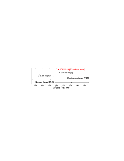
Figure 1: (Color online) Different determinations of the difference of the squared nuclear charge radii of ³He and ⁴He.

Table 8: Hyperfine splitting of the $2^{3}S$ state of ³He, in kHz.

$H^{(4+)}$	$6\,740\,451.46$
$H^{(6)}$	$-1\,313.99$
$(H^{(4)}_{\rm hfs},H^{(4)}_{\rm nfs}+H^{(4)}_{\rm fs})$	$2\,189.81$
$(H^{(4)}_{\rm hfs},H^{(4)}_{\rm hfs})$	$-60.52\pm 1.7$
$H_{\rm nucl\&ho}$	$-1\,566.83$
Total	$6\,739\,699.93\pm 1.7$
Experiment rosner:70	$6\,739\,701.177\,(16)$

Table 9: Determination of the difference of the mean square nuclear charge radii $\delta r^{2}$ of ³He and ⁴He from the measurement by Shiner et al. shiner:95 . The remainder $\delta E$ is proportinal to $\delta r^{2}$, $\delta E=C\,\delta r^{2}$, with $C=-1212.2(1)$ kHz/fm², see text for details. Units are kHz.

$E(^{3}{\rm He},2^{3}P_{0}^{1/2}-2^{3}S_{1}^{3/2})-E(^{4}{\rm He},2^{3}P_{2}-2^{3}S_{1})$	$810\,599.(3.)$	Experiment shiner:95
$\delta E_{\rm hfs}(2^{3}S_{1}^{3/2})$	$-2\,246\,567.059(5)$	Experiment schluesser:69
$\delta E_{\rm fs}(2^{3}P_{2})$	$-4\,309\,074.2(1.7)$	Theory, pachucki:10:hefs and this work, Eq. (54)
$-\delta E_{\rm hfs}(2^{3}P_{0}^{1/2})$	$-27\,923\,393.7\,(1.7)$	Theory, this work, Table VIII
$-\delta E_{\rm iso}(2^{3}P-2^{3}S)$ (point nucleus)	$33\,667\,143.2(3.9)$	Theory cancio:12:3he
$\delta E$	$-1\,292.8(5.2)$

IX Summary

In summary, we have calculated the mixed hyperfine and fine structure of the $2^{3}P$ states of ³He. Our investigation advances the previous theory by a complete calculation of the $m\alpha^{6}$ correction, which leads to an order-of-magnitude improvement in accuracy. Theoretical predictions for most of the transitions are accurate to better than 2 kHz. The $2^{3}P_{1}^{1/2}$-$2^{3}P_{1}^{3/2}$ transition is calculated up to 0.9 kHz, which is currently the most precise theoretical result for the helium transitions. Both the hypefine and fine-structure transitions are in good agreement with measurements by Cancio et al. cancio:12:3he and by Smiciklas smiciklas:03 .

Since the present theoretical accuracy for the fine-structure transitions in ³He is comparable to that for ⁴He, one can in principle use the ³He spectroscopy for the determination of the fine structure constant $\alpha$, as in was done for ⁴He in Ref. pachucki:10:hefs . However, such determination does not bring much advantage at present, since the experimental accuracy for ³He is lower than for ⁴He borbely:09 ; smiciklas:10 . Because of this, we do not determine $\alpha$ from the ³He transitions in this work. However, if the experimental precision of the ³He hyperfine structure is improved to the sub-kHz level, one will be able to use these results for the spectropic determination of the fine structure constant.

Another application of the hyperfine structure measurements in ³He might be determination of the dipole magnetic moment of helion. The principal problem here is that the present theory obtains the nuclear-structure contribution from the experimental value of the hyperfine splitting in ³He⁺. This greatly reduces the sensitivity of the final theoretical prediction on the nuclear magnetic moment. Our calculation shows that at present, the hyperfine structure of ³He allows for determination of the dipole magnetic moment of helion with an accuracy of about $5\times 10^{-5}$ only.

Appendix A Angular-momentum matrix elements

In this section we calculate the matrix elements of the basic angular-momentum operators that are relevant for the present work. The angular-momentum algebra is conveniently done with formulas from Ref. varshalovich . The results are

$$\langle FIJLSM_{F}|\vec{I}\cdot\vec{S}|FIJ^{\prime}L^{\prime}S^{\prime}M_{F}\rangle \ =(-1)^{I+J+F}\,\left\{\begin{array}[]{ccc}I&J&F\\ J^{\prime}&I&1\\ \end{array}\right\}\,\sqrt{I(I+1)(2I+1)}\,$$ (60)

$$\times\delta_{L,L^{\prime}}\,\delta_{S,S^{\prime}}\,(-1)^{L+S+J+1}\,\sqrt{S(S+1)(2S+1)(2J+1)(2J^{\prime}+1)}\,\left\{\begin{array}[]{ccc}S&L&J^{\prime}\\ J&1&S\\ \end{array}\right\}\,,$$ (63)

$$\langle FIJLSM_{F}|\vec{I}\cdot\vec{L}|FIJ^{\prime}L^{\prime}S^{\prime}M_{F}\rangle \ =(-1)^{I+J+F}\,\left\{\begin{array}[]{ccc}I&J&F\\ J^{\prime}&I&1\\ \end{array}\right\}\,\sqrt{I(I+1)(2I+1)}\,$$ (66)

$$\times\delta_{L,L^{\prime}}\,\delta_{S,S^{\prime}}\,(-1)^{L+S+J^{\prime}+1}\,\sqrt{L(L+1)(2L+1)(2J+1)(2J^{\prime}+1)}\,\left\{\begin{array}[]{ccc}L&S&J\\ J^{\prime}&1&L\\ \end{array}\right\}\,,$$ (69)

$$\langle I^{i}\,S^{j}\,(L^{i}\,L^{j})^{(2)}\rangle=\frac{1}{4}\left[J(J+1)+J^{\prime}(J^{\prime}+1)-2L(L+1)-2S(S+1)\right]\,\langle\vec{I}\cdot\vec{L}\rangle-\frac{1}{3}\,L(L+1)\,\langle\vec{I}\cdot\vec{S}\rangle\,,$$ (70)

$$\langle I^{i}\,L^{j}\,(S^{i}\,S^{j})^{(2)}\rangle=\frac{1}{4}\left[J(J+1)+J^{\prime}(J^{\prime}+1)-2L(L+1)-2S(S+1)\right]\,\langle\vec{I}\cdot\vec{S}\rangle-\frac{1}{3}\,S(S+1)\,\langle\vec{I}\cdot\vec{L}\rangle\,,$$ (71)

$$\langle(S^{i}\,S^{j})^{(2)}(L^{i}\,L^{j})^{(2)}\rangle=\langle\vec{L}\cdot\vec{S}\rangle^{2}+\frac{1}{2}\,\langle\vec{L}\cdot\vec{S}\rangle-\frac{L\,(L+1)\,S\,(S+1)}{3}\,.$$ (72)

Appendix B Derivation of $H_{\rm hfs}^{(6)}$

We start with the Breit Hamiltonian $H_{BP}$ of the atomic system in the external magnetic field,

$$H_{BP} = \sum_{a}H_{a}+\sum_{a,b;a>b}H_{ab}\,$$ (73)

$$H_{a} = \frac{\vec{\pi}_{a}^{2}}{2\,m}-\frac{Z\,\alpha}{r_{a}}-\frac{e}{2\,m}\,\vec{\sigma}_{a}\cdot\vec{B}_{a}-\frac{\vec{\pi}_{a}^{4}}{8\,m^{3}}+\frac{\pi\,Z\,\alpha}{2\,m^{2}}\,\delta^{3}(r_{a})+\frac{Z\,\alpha}{4\,m^{2}}\,\vec{\sigma}_{a}\cdot\frac{\vec{r}_{a}}{r_{a}^{3}}\times\vec{\pi}_{a}$$ (74)

$$+\frac{e}{8\,m^{3}}\,\bigl{(}\vec{\sigma}_{a}\cdot\vec{B}_{a}\,\vec{\pi}_{a}^{2}+\vec{\pi}_{a}^{2}\,\vec{\sigma}_{a}\cdot\vec{B}_{a}\bigr{)}\,,$$

$$H_{ab} = \frac{\alpha}{r_{ab}}+\frac{\pi\,\alpha}{m^{2}}\,\delta^{3}(r_{ab})-\frac{\alpha}{2\,m^{2}}\,\pi_{a}^{i}\,\biggl{(}\frac{\delta^{ij}}{r_{ab}}+\frac{r_{ab}^{i}\,r_{ab}^{j}}{r_{ab}^{2}}\biggr{)}\,\pi_{b}^{j}$$ (75)

$$+\frac{\alpha}{4\,m^{2}r_{ab}^{3}}\bigl{[}\vec{\sigma}_{a}\cdot\vec{r}_{ab}\times(2\,\vec{\pi}_{b}-\vec{\pi}_{a})-\vec{\sigma}_{b}\cdot\vec{r}_{ab}\times(2\,\vec{\pi}_{a}-\vec{\pi}_{b})\bigr{]}$$

$$+\frac{\alpha}{4\,m^{2}}\,\frac{\sigma_{a}^{i}\,\sigma_{b}^{j}}{r_{ab}^{3}}\,\biggl{(}\delta^{ij}-3\,\frac{r_{ab}^{i}\,r_{ab}^{j}}{r_{ab}^{2}}\biggr{)}\,,$$

where $\vec{\pi}=\vec{p}-e\,\vec{A}$. Magnetic fields $\vec{A}$ and $\vec{B}$ induced by the nuclear magnetic moment are

$$e\,\vec{A}(\vec{r}) = \frac{e}{4\,\pi}\,\vec{\mu}\times\frac{\vec{r}}{r^{3}}=-Z\,\alpha\,\frac{(1+\kappa)}{M}\,\vec{I}\times\frac{\vec{r}}{r^{3}}\,,$$ (76)

$$e\,\vec{B}^{i}(\vec{r}) = \bigl{(}\vec{\nabla}\times\vec{A}\bigr{)}^{i}=-Z\,\alpha\,\frac{(1+\kappa)}{M}\,\frac{8\,\pi}{3}\,\delta^{3}(r)\,I^{i}+Z\,\alpha\,\frac{(1+\kappa)}{M}\,\frac{1}{r^{3}}\,\biggl{(}\delta^{ij}-3\,\frac{r^{i}\,r^{j}}{r^{2}}\biggr{)}\,I^{j}\,.$$ (77)

The leading-order interaction between the nuclear spin $\vec{I}$ and the electron spin $\vec{\sigma}_{a}$ is obtained from the nonrelativistic terms $\nicefrac{{1}}{{2\,m}}\,\vec{\pi}_{a}^{2}$ and $\nicefrac{{e}}{{2\,m}}\,\vec{\sigma}_{a}\cdot\vec{B}_{a}$, yielding

$$H^{(4)}_{\rm hfs}=-\sum_{a}\biggl{[}\frac{e}{m}\,\vec{p}_{a}\cdot\vec{A}(\vec{r}_{a})-\frac{e}{2\,m}\,\vec{\sigma}_{a}\cdot\vec{B}(\vec{r}_{a})\biggr{]}\,,$$ (78)

in agreement with Eq. (5). The relativistic correction to the hyperfine interaction is similarly obtained from the relativistic terms in the Breit Hamiltonian $H_{BP}$,

$$H^{(6)}_{\rm hfs} = \sum_{a}\frac{Z\,\alpha}{4\,m^{2}}\,\vec{\sigma}_{a}\cdot\frac{\vec{r}_{a}}{r_{a}^{3}}\times\bigl{[}-e\,\vec{A}(\vec{r}_{a})\bigr{]}+\frac{e}{8\,m^{3}}\,\bigl{(}\vec{\sigma}_{a}\cdot\vec{B}_{a}\,\vec{p}_{a}^{\,2}+\vec{p}_{a}^{\,2}\,\vec{\sigma}_{a}\cdot\vec{B}_{a}\bigr{)}$$ (80)

$$+\sum_{a,b;a\neq b}\frac{\alpha}{4\,m^{2}r_{ab}^{3}}\,\vec{\sigma}_{a}\cdot\vec{r}_{ab}\times\bigl{[}-2\,e\,\vec{A}(\vec{r}_{b})+e\,\vec{A}(\vec{r}_{a})\bigr{]}$$

$$+\frac{e}{4\,m^{3}}\,\sum_{a}\bigl{[}\vec{p}_{a}^{\;2}\,\vec{p}_{a}\cdot\vec{A}(\vec{r}_{a})+\vec{p}_{a}\cdot\vec{A}(\vec{r}_{a})\,\vec{p}_{a}^{\;2}\bigr{]}-\sum_{a\neq b}\frac{\alpha}{2\,m^{2}}\,p_{a}^{i}\,\biggl{(}\frac{\delta^{ij}}{r_{ab}}+\frac{r_{ab}^{i}\,r_{ab}^{j}}{r_{ab}^{3}}\biggr{)}\,\bigl{[}-\,e\,A^{j}(\vec{r}_{b})\bigr{]}\,.$$

Using $\vec{A}$ and $\vec{B}$ from Eqs. (76) and (77), we derive Eq. (IV).

Appendix C Second order matrix elements

The second-order $m\alpha^{6}$ correction $\delta E_{\rm sec}$ [see Eq. (22)] is split into several parts in accordance with the symmetry of the intermediate states,

$$\delta E_{\rm sec}=\frac{m_{r}^{3}}{m\,M}\,(1+\kappa)\,\alpha^{6}\,\biggl{[}\delta E_{\rm sing}(^{3}P)+\delta E_{\rm reg}(^{3}P)+\delta E(^{1}P)+\delta E(^{3}D)+\delta E(^{1}D)+\delta E(^{3}F)\biggr{]}\,.$$ (81)

The angular momentum algebra for different intermediate states is simple but rather tedious and is performed with help of the symbolic algebra computer program. Below we list the resulting formulas expressed in a form convenient for the numerical evaluation.

The singular part with the ${}^{3}P$ intermediate states is given by (after removing all divergencies)

$$\delta E_{\rm sing}(^{3}P)=\biggl{\langle}Q^{\prime}\,\frac{1}{(E-H)^{\prime}}\,T^{\prime}\biggr{\rangle}\,2\,\langle\vec{I}\cdot\vec{S}\rangle\,,$$ (82)

where $E\equiv E(2^{3}P)$,

$$Q^{\prime} \equiv Q+\frac{2}{3}\,\sum_{a}\,\biggl{\{}\frac{Z}{r_{a}}\,,\,E-H\biggr{\}}=-\frac{2\,Z}{3}\,\biggl{(}\frac{\vec{r}_{1}}{r_{1}^{3}}\cdot\vec{\nabla}_{1}+\frac{\vec{r}_{2}}{r_{2}^{3}}\cdot\vec{\nabla}_{2}\biggr{)}\,,$$ (83)

$$T^{\prime} \equiv T-\frac{1}{4}\,\sum_{a}\,\biggl{\{}\frac{Z}{r_{a}}\,,\,E-H\biggr{\}}=-\frac{1}{2}\,\left(E+\frac{Z}{r_{1}}+\frac{Z}{r_{2}}-\frac{1}{r}\right)^{2}-p_{1}^{i}\,\frac{1}{2\,r}\,\biggl{(}\delta^{ij}+\frac{r^{i}\,r^{j}}{r^{2}}\biggr{)}\,p_{2}^{j}$$ (84)

$$\ \ \ \ \ \ \ \ \ \ \ \ \ \ \ \ \ \ \ \ \ \ \ \ \ \ \ \ \ \ \ \ \ \ \ +\frac{1}{4}\,\vec{\nabla}_{1}^{2}\,\vec{\nabla}_{2}^{2}-\frac{Z}{4}\,\frac{\vec{r}_{1}}{r_{1}^{3}}\cdot\vec{\nabla}_{1}-\frac{Z}{4}\,\frac{\vec{r}_{2}}{r_{2}^{3}}\cdot\vec{\nabla}_{2}+\frac{1}{2}\,\frac{\vec{r}}{r^{3}}\cdot(\vec{\nabla}_{1}-\vec{\nabla}_{2})\,,$$

and it is assumed that the operators $T^{\prime}$ and $Q^{\prime}$ act on the function on the right hand side that satisfies the Schrödinger equation with the energy $E$.

The regular part with the ${}^{3}P$ intermediate states is

$$\delta E_{\rm reg}(^{3}P) = \sum_{n>2}\,\frac{1}{E(2^{3}P)-E(n^{3}P)}\biggl{[}\langle 2^{3}\vec{P}|Q|n^{3}\vec{P}\rangle\,\langle n^{3}\vec{P}|\vec{T}|2^{3}\vec{P}\rangle\,\langle\frac{2}{3}\,\vec{I}\cdot\vec{L}+I^{i}\,L^{j}\,(S^{i}\,S^{j})^{(2)}\rangle$$ (85)

$$+\langle 2^{3}\vec{P}|Q|n^{3}\vec{P}\rangle\,\langle n^{3}\vec{P}|\hat{T}|2^{3}\vec{P}\rangle\,\langle-\frac{3}{5}\,I^{i}\,S^{j}\,(L^{i}\,L^{j})^{(2)}\rangle+\langle 2^{3}\vec{P}|\vec{Q}|n^{3}\vec{P}\rangle\,\langle n^{3}\vec{P}|T|2^{3}\vec{P}\rangle\,\langle\vec{I}\cdot\vec{L}\rangle$$

$$+\langle 2^{3}\vec{P}|\vec{Q}|n^{3}\vec{P}\rangle\,\langle n^{3}\vec{P}|\vec{T}|2^{3}\vec{P}\rangle\,\langle\frac{1}{3}\,\vec{I}\cdot\vec{S}+\frac{1}{2}\,I^{i}\,S^{j}\,(L^{i}\,L^{j})^{(2)}\rangle$$

$$+\langle 2^{3}\vec{P}|\vec{Q}|n^{3}\vec{P}\rangle\,\langle n^{3}\vec{P}|\hat{T}|2^{3}\vec{P}\rangle\,\langle-\frac{3}{10}\,I^{i}\,L^{j}\,(S^{i}\,S^{j})^{(2)}\rangle$$

$$+\langle 2^{3}\vec{P}|\hat{Q}|n^{3}\vec{P}\rangle\,\langle n^{3}\vec{P}|T|2^{3}\vec{P}\rangle\,\langle-\frac{6}{5}\,\,I^{i}\,S^{j}\,(L^{i}\,L^{j})^{(2)}\rangle$$

$$+\langle 2^{3}\vec{P}|\hat{Q}|n^{3}\vec{P}\rangle\,\langle n^{3}\vec{P}|\vec{T}|2^{3}\vec{P}\rangle\,\langle-\frac{1}{3}\,\vec{I}\cdot\vec{L}+\frac{9}{20}\,I^{i}\,S^{j}\,(L^{i}\,L^{j})^{(2)}-\frac{1}{20}\,I^{i}\,L^{j}\,(S^{i}\,S^{j})^{(2)}\rangle$$

$$+\langle 2^{3}\vec{P}|\hat{Q}|n^{3}\vec{P}\rangle\,\langle n^{3}\vec{P}|\hat{T}|2^{3}\vec{P}\rangle\,\langle\frac{1}{5}\,\vec{I}\cdot\vec{S}-\frac{21}{100}\,I^{i}\,S^{j}\,(L^{i}\,L^{j})^{(2)}-\frac{27}{100}\,I^{i}\,L^{j}\,(S^{i}\,S^{j})^{(2)}\rangle\biggr{]}\,.$$

The other parts are

$$\delta E(^{1}P)= \ \sum_{n}\,\frac{1}{E(2^{3}P)-E(n^{1}P)}\biggl{[}\langle 2^{3}\vec{P}|Q_{A}|n^{1}\vec{P}\rangle\,\langle n^{1}\vec{P}|\vec{T}_{A}|2^{3}\vec{P}\rangle\,\langle\frac{1}{3}\,\vec{I}\cdot\vec{L}-I^{i}\,L^{j}\,(S^{i}\,S^{j})^{(2)}\rangle$$

$$+\langle 2^{3}\vec{P}|\hat{Q}_{A}|n^{1}\vec{P}\rangle\,\langle n^{1}\vec{P}|\vec{T}_{A}|2^{3}\vec{P}\rangle\,\langle-\frac{1}{6}\,\vec{I}\cdot\vec{L}+\frac{9}{20}\,I^{i}\,S^{j}\,(L^{i}\,L^{j})^{(2)}+\frac{1}{20}\,I^{i}\,L^{j}\,(S^{i}\,S^{j})^{(2)}\rangle\biggr{]}\,,$$ (86)

$$\delta E(^{3}D) \ =\sum_{n}\,\frac{1}{E(2^{3}P)-E(n^{3}D)}\biggl{[}\langle 2^{3}\vec{P}|\vec{Q}|n^{3}\hat{D}\rangle\,\langle n^{3}\hat{D}|\vec{T}|2^{3}\vec{P}\rangle\,\langle\frac{2}{3}\,\vec{I}\cdot\vec{S}-\frac{1}{5}\,I^{i}\,S^{j}\,(L^{i}\,L^{j})^{(2)}\rangle$$

$$+\langle 2^{3}\vec{P}|\hat{Q}|n^{3}\hat{D}\rangle\,\langle n^{3}\hat{D}|\hat{T}|2^{3}\vec{P}\rangle\,\langle\frac{2}{9}\,\vec{I}\cdot\vec{S}+\frac{7}{30}\,I^{i}\,S^{j}\,(L^{i}\,L^{j})^{(2)}-\frac{1}{10}\,I^{i}\,L^{j}\,(S^{i}\,S^{j})^{(2)}\rangle$$

$$+\langle 2^{3}\vec{P}|\hat{Q}|n^{3}\hat{D}\rangle\,\langle n^{3}\hat{D}|\vec{T}|2^{3}\vec{P}\rangle\,\langle-\frac{2}{3}\,\vec{I}\cdot\vec{L}-\frac{3}{10}\,I^{i}\,S^{j}\,(L^{i}\,L^{j})^{(2)}-\frac{1}{10}\,I^{i}\,L^{j}\,(S^{i}\,S^{j})^{(2)}\rangle$$

$$+\langle 2^{3}\vec{P}|\vec{Q}|n^{3}\hat{D}\rangle\,\langle n^{3}\hat{D}|\hat{T}|2^{3}\vec{P}\rangle\,\,\langle-\frac{3}{5}I^{i}\,L^{j}\,(S^{i}\,S^{j})^{(2)}\rangle\biggr{]}\,,$$ (87)

$$\delta E(^{1}D) \ =\sum_{n}\,\frac{1}{E(2^{3}P)-E(n^{1}D)}\,\langle 2^{3}\vec{P}|\hat{Q}_{A}|n^{1}\hat{D}\rangle\,\langle n^{3}\hat{D}|\vec{T}_{A}|2^{1}\vec{P}\rangle\langle-\frac{1}{3}\,\vec{I}\cdot\vec{L}-\frac{3}{10}\,I^{i}\,S^{j}\,(L^{i}\,L^{j})^{(2)}+\frac{1}{10}\,I^{i}\,L^{j}\,(S^{i}\,S^{j})^{(2)}\rangle\,,$$ (88)

$$\delta E(^{3}F) \ =\sum_{n}\,\frac{1}{E(2^{3}P)-E(n^{3}F)}\,\langle 2^{3}\vec{P}|\hat{Q}|n^{3}\tilde{F}\rangle\,\langle n^{3}\tilde{F}|\hat{T}|2^{3}\vec{P}\rangle\langle\frac{1}{3}\,\vec{I}\cdot\vec{S}-\frac{1}{10}\,I^{i}\,S^{j}\,(L^{i}\,L^{j})^{(2)}+\frac{3}{10}\,I^{i}\,L^{j}\,(S^{i}\,S^{j})^{(2)}\rangle\,.$$ (89)

The matrix elements with the $D$ and $F$-state wave functions are defined by

$$\langle\vec{\phi}|\vec{Q}|\hat{\psi}\rangle \equiv -i\,\langle\phi_{i}|Q_{j}|\psi_{ij}\rangle=i\,\langle\psi_{ij}|Q_{j}|\phi_{i}\rangle\equiv\langle\hat{\psi}|\vec{Q}|\vec{\phi}\rangle\,,$$ (90)

$$\langle\vec{\phi}|\hat{Q}|\hat{\psi}\rangle \equiv \epsilon^{ijk}\langle\phi_{i}|Q_{jl}|\psi_{kl}\rangle=\epsilon^{ijk}\langle\psi_{kl}|Q_{jl}|\phi_{i}\rangle\equiv\langle\hat{\psi}|\hat{Q}|\vec{\phi}\rangle\,,$$ (91)

$$\langle\vec{\phi}|\hat{Q}|\tilde{\psi}\rangle \equiv \langle\phi_{i}|Q_{jk}|\psi_{ijk}\rangle=\langle\psi_{ijk}|Q_{ij}|\phi_{k}\rangle\equiv\langle\tilde{\psi}|\hat{Q}|\hat{\phi}\rangle\,,$$ (92)

where $\hat{\psi}$ denotes the odd $D$ wave function,

$$\psi^{ij}=\left(\epsilon^{ikl}r_{1}^{k}r_{2}^{l}r_{1}^{j}+\epsilon^{jkl}r_{1}^{k}r_{2}^{l}r_{1}^{i}\right)\,f(r_{1},r_{2},r)\pm(r_{1}\leftrightarrow r_{2})\,,$$ (93)

and $\tilde{\psi}$ denotes the odd $F$ wave function,

$$\psi^{ijk}= \ \left[r_{1}^{i}r_{1}^{j}r_{1}^{k}-\frac{r_{1}^{2}}{5}\left(\delta_{ij}r_{1}^{k}+\delta_{ik}r_{1}^{i}+\delta_{jk}r_{1}^{i}\right)\right]\,f(r_{1},r_{2},r)+\frac{1}{3}\biggl{[}r_{1}^{i}r_{1}^{j}r_{2}^{k}+r_{1}^{i}r_{2}^{j}r_{1}^{k}+r_{2}^{i}r_{1}^{j}r_{1}^{k}$$

$$-\frac{\delta_{ij}}{5}(r_{1}^{2}r_{2}^{k}+2r_{1}^{l}r_{2}^{l}r_{1}^{k})-\frac{\delta_{ik}}{5}(r_{1}^{2}r_{2}^{j}+2r_{1}^{l}r_{2}^{l}r_{1}^{j})-\frac{\delta_{jk}}{5}(r_{1}^{2}r_{2}^{i}+2r_{1}^{l}r_{2}^{l}r_{1}^{i})\biggr{]}\,g(r_{1},r_{2},r)\pm(r_{1}\leftrightarrow r_{2})\,.$$ (94)

All wave functions are real and normalized by $\langle\psi^{i}|\psi^{i}\rangle=\langle\psi^{ij}|\psi^{ij}\rangle=\langle\psi^{ijk}|\psi^{ijk}\rangle=1$.

The second-order corrections listed above are finite. However, some matrix elements are too singular for the direct numerical evaluation and need to be transformed to a more regular form. The regularization method is described in Sec. IV. So, the operator $T$ is transformed by Eq. (32), thus yielding

$$\sum_{n>2}\,\frac{1}{E(2^{3}P)-E(n^{3}P)}\langle 2^{3}\vec{P}|\vec{Q}|n^{3}\vec{P}\rangle\,\langle n^{3}\vec{P}|T|2^{3}\vec{P}\rangle$$

$$=\sum_{n>2}\,\frac{1}{E(2^{3}P)-E(n^{3}P)}\langle 2^{3}\vec{P}|\vec{Q}|n^{3}\vec{P}\rangle\,\langle n^{3}\vec{P}|T^{\prime}|2^{3}\vec{P}\rangle+\langle 2^{3}\vec{P}|\frac{1}{4}\,\sum_{a}\frac{Z}{r_{a}}\,\vec{Q}\,|2^{3}\vec{P}\rangle-\langle 2^{3}\vec{P}|\frac{1}{4}\,\sum_{a}\frac{Z}{r_{a}}|2^{3}\vec{P}\rangle\,\langle 2^{3}\vec{P}|\vec{Q}\,|2^{3}\vec{P}\rangle\,.$$ (95)

We observe that, after the transformation, the singular part of the operator $T$ is absorbed in the first-order matrix element, whereas the second-order correction contains only the (more regular) operator $T^{\prime}$.

Similarly, the operator $Q^{ij}$ is transformed by

$$Q^{\prime ij} \equiv Q^{ij}-\bigl{\{}\delta Q^{ij}\,,\,E-H\bigr{\}}=-\frac{Z}{6}\,\sum_{a}\biggl{(}-\delta^{ij}\,\frac{r_{a}^{k}}{r_{a}^{3}}-3\,\delta^{ik}\,\frac{r_{a}^{j}}{r_{a}^{3}}-3\,\delta^{jk}\,\frac{r_{a}^{i}}{r_{a}^{3}}+9\,\frac{r_{a}^{i}\,r_{a}^{j}\,r_{a}^{k}}{r_{a}^{5}}\biggr{)}\,\nabla_{a}^{k}\,,$$ (96)

where $E\equiv E(2^{3}P)$,

$$\delta Q^{ij}=\frac{1}{6}\,\sum_{a}\,\frac{Z}{r_{a}}\,\biggl{(}\delta^{ij}-3\frac{r_{a}^{i}\,r_{a}^{j}}{r_{a}^{2}}\biggr{)}\,$$ (97)

and it is assumed that the function on the right hand side of $\hat{Q}^{\prime}$ satisfies the Schrödinger align with energy $E$. The second-order matrix elements with $Q^{ij}$ then are transformed by

$$\sum_{n>2}\,\frac{1}{E(2^{3}P)-E(n^{3}P)}\langle 2^{3}\vec{P}|\hat{Q}|n^{3}\vec{P}\rangle\,\langle n^{3}\vec{P}|\vec{T}|2^{3}\vec{P}\rangle$$

$$=\sum_{n>2}\,\frac{1}{E(2^{3}P)-E(n^{3}P)}\langle 2^{3}\vec{P}|\hat{Q}^{\prime}|n^{3}\vec{P}\rangle\,\langle n^{3}\vec{P}|\vec{T}|2^{3}\vec{P}\rangle+\left(-i\epsilon^{klm}\right)\langle 2^{3}P_{i}|\delta Q_{ik}\,T_{l}\,|2^{3}P_{m}\rangle-\langle 2^{3}\vec{P}|\delta\hat{Q}|2^{3}\vec{P}\rangle\,\langle 2^{3}\vec{P}|\vec{T}\,|2^{3}\vec{P}\rangle\,,$$ (98)

and

$$\sum_{n>2}\,\frac{1}{E(2^{3}P)-E(n^{3}P)}\langle 2^{3}\vec{P}|\hat{Q}|n^{3}\vec{P}\rangle\,\langle n^{3}\vec{P}|T|2^{3}\vec{P}\rangle=\sum_{n>2}\,\frac{1}{E(2^{3}P)-E(n^{3}P)}\langle 2^{3}\vec{P}|\hat{Q}^{\prime}|n^{3}\vec{P}\rangle\,\langle n^{3}\vec{P}|T^{\prime}|2^{3}\vec{P}\rangle$$

$$+\langle 2^{3}\vec{P}|\frac{1}{4}\,\sum_{a}\frac{Z}{r_{a}}\,\hat{Q}\,|2^{3}\vec{P}\rangle-\langle 2^{3}\vec{P}|\frac{1}{4}\,\sum_{a}\frac{Z}{r_{a}}|2^{3}\vec{P}\rangle\,\langle 2^{3}\vec{P}|\hat{Q}|2^{3}\vec{P}\rangle+\langle 2^{3}\vec{P}|\delta\hat{Q}\,T^{\prime}|2^{3}\vec{P}\rangle-\langle 2^{3}\vec{P}|\delta\hat{Q}|2^{3}\vec{P}\rangle\,\langle 2^{3}\vec{P}|T^{\prime}|2^{3}\vec{P}\rangle\,.$$ (99)

The operator $Q_{A}$ is transformed as

$$Q^{\prime}_{A} \equiv Q_{A}+\frac{2}{3}\,\biggl{\{}\frac{Z}{r_{1}}-\frac{Z}{r_{2}}\,,\,E-H\biggr{\}}=\frac{2\,Z}{3}\,\biggl{(}-\frac{\vec{r}_{1}}{r_{1}^{3}}\cdot\vec{\nabla}_{1}+\frac{\vec{r}_{2}}{r_{2}^{3}}\cdot\vec{\nabla}_{2}\biggr{)}\,,$$ (100)

where it is assumed that the function on the right hand side of $Q^{\prime}_{A}$ satisfies the Schrödinger equation with the energy $E$. The regularized form of the second-order matrix element then is

$$\sum_{n}\,\displaystyle{\frac{1}{E(2^{3}P)-E(n^{1}P)}}\,\langle 2^{3}\vec{P}|Q_{A}|n^{1}\vec{P}\rangle\,\langle n^{1}\vec{P}|\vec{T}_{A}|2^{3}\vec{P}\rangle=$$

$$\sum_{n}\,\displaystyle{\frac{1}{E(2^{3}P)-E(n^{1}P)}}\,\langle 2^{3}\vec{P}|Q^{\prime}_{A}|n^{1}\vec{P}\rangle\,\langle n^{1}\vec{P}|\vec{T}_{A}|2^{3}\vec{P}\rangle-\frac{2}{3}\,\langle 2^{3}\vec{P}|\left(\frac{Z}{r_{1}}-\frac{Z}{r_{2}}\right)\vec{T}_{A}|2^{3}\vec{P}\rangle\,.$$ (101)

References

- (1) K. Pachucki and V. A. Yerokhin, Phys. Rev. Lett. 104, 070403 (2010).
- (2) D. Hanneke, S. Fogwell, and G. Gabrielse, Phys. Rev. Lett. 100, 120801 (2008).
- (3) R. Bouchendira, P. Cladé, S. Guellati-Khélifa, F. Nez, and F. Biraben, Phys. Rev. Lett. 106, 080801 (2011).
- (4) R. van Rooij, J. S. Borbely, J. Simonet, M. Hoogerland, K. S. E. Eikema, R. A. Rozendaal, and W. Vassen, Science 333, 196 (2011).
- (5) P. Cancio Pastor, L. Consolino, G. Giusfredi, P. De Natale, M. Inguscio, V. A. Yerokhin, and K. Pachucki, Phys. Rev. Lett. 108, 143001 (2012).
- (6) P. Cancio Pastor et al. Phys. Rev. Lett. 92, 023001 (2004), [(E) ibid 97, 139903 (2006)].
- (7) I. Sick, Lect. Notes Phys. 745, 57 (2008).
- (8) R. Pohl et al., Nature (London) 466, 213 (2010).
- (9) A. Antognini et al., Can. J. Phys. 89, 47 (2011).
- (10) D. Shiner, R. Dixon, and V. Vedantham, Phys. Rev. Lett. 74, 3553 (1995).
- (11) D. Morton, Q. Wu, and G. W. F. Drake, Phys. Rev. A 73, 034502 (2006).
- (12) Q. Wu and G. W. F. Drake, J. Phys. B 40, 393 (2007).
- (13) M. Smiciklas, Master thesis, University of North Texas, unpublished, 2003; arXiv:physics/1203.2830.
- (14) K. Pachucki, J. Phys. B 34, 3357 (2001).
- (15) F. Marin, F. Minardi, F. S. Pavone, M. Inguscio, and G. W. F. Drake, Z. Phys. D 32, 285 (1995).
- (16) H. A. Schluesser, E. N. Fortson, and H. G. Dehmelt, Phys. Rev. 187, 5 (1969), [(E) Phys. Rev. A 2, 1612 (1970)].
- (17) K. Pachucki and V. A. Yerokhin, Phys. Rev. A 79, 062516 (2009), [ibid. 80, 019902(E) (2009); ibid. 81, 039903(E) (2010)].
- (18) CODATA internationally recommended values of the fundamental physical constants, http://physics.nist.gov/cuu/Constants.
- (19) L. Consolino et al. Opt. Express 19, 3155 (2011).
- (20) S. D. Rosner and F. M. Pipkin, Phys. Rev. A 1, 571 (1970), [(E) Phys. Rev. A 3, 521 (1971)].
- (21) J. S. Borbely, M. C. George, L. D. Lombardi, M. Weel, D. W. Fitzakerley, and E. A. Hessels, Phys. Rev. A 79, 0605030(R) (2009).
- (22) M. Smiciklas and D. Shiner, Phys. Rev. Lett. 105, 123001 (2010).
- (23) G. Drake, W. Nörtershäuser, and Z.-C. Yan, Can. J. Phys. 83, 311 (2005).
- (24) I. Sick, Phys. Rev. C 77, 041302 (2008).
- (25) A. Kievsky et al. J. Phys. G 35, 063101 (2008).
- (26) D. A. Varshalovich, A. N. Moskalev, and V. K. Khersonskiĭ, Quantum Theory of Angular Momentum, World Scientific, Singapure, 1988.