Analysis of complex contagions in random multiplex networks

Abstract

We study the diffusion of influence in random multiplex networks where links can be of $r$ different types, and for a given content (e.g., rumor, product, political view), each link type is associated with a content dependent parameter $c_{i}$ in $[0,\infty]$ that measures the relative bias type-$i$ links have in spreading this content. In this setting, we propose a linear threshold model of contagion where nodes switch state if their “perceived” proportion of active neighbors exceeds a threshold $\tau$. Namely, a node connected to $m_{i}$ active neighbors and $k_{i}-m_{i}$ inactive neighbors via type-$i$ links will turn active if $\sum{c_{i}m_{i}}/\sum{c_{i}k_{i}}$ exceeds its threshold $\tau$. Under this model, we obtain the condition, probability and expected size of global spreading events. Our results extend the existing work on complex contagions in several directions by (i) providing solutions for coupled random networks whose vertices are neither identical nor disjoint, (ii) highlighting the effect of content on the dynamics of complex contagions, and (iii) showing that content-dependent propagation over a multiplex network leads to a subtle relation between the giant vulnerable component of the graph and the global cascade condition that is not seen in the existing models in the literature.

PACS numbers

89.75.Hc, 87.23.Ge

I Introduction

In the past decade, there has been an increasing interest in studying dynamical processes on real-world complex networks. An interesting phenomenon that seems to occur in many such processes is the spreading of an initially localized effect throughout the whole (or, a very large part of the) network. These events are usually referred to as (information) cascades and can be observed in processes as diverse as adoption of cultural fads, the diffusion of belief, norms, and innovations in social networks Watts (2002); Dodds and Watts (2004); Duan et al. (2005), disease contagion in human and animal populations Murray (2002); Anderson and May (1991), failures in interdependent infrastructures Buldyrev et al. (2010, 2011); Cho et al. (2010); Cohen and Havlin (2010); Huang et al. (2011); Shao et al. (2011); Vespignani (2010); Yağan et al. (2012, 2011a), rise of collective action to join a riot Granovetter (1978), and global spread of computer viruses or worms on the Web Newman et al. (2002); Balthrop et al. (2004).

The current paper focuses on a class of dynamic processes usually known as binary decisions with externalities Watts (2002). In this model, nodes can be in either one of the two states: active or inactive. Each node is initially given a random threshold $\tau$ in $(0,1]$ drawn independently from a distribution $P_{\textrm{th}}(\tau)$. Then, starting from a small number of active vertices, nodes update their states (synchronously) in discrete time steps. An inactive node with $m$ active neighbors and $k-m$ inactive neighbors will be activated only if the fraction $\frac{m}{k}$ exceeds $\tau$; once active, a node can not be deactivated. This model is sometimes referred to as the Watts’ threshold model. However, it was motivated by the seminal work of Schelling Schelling (1973) who employed a threshold model to gain insight into residential segregation. Granovetter Granovetter (1978) also studied this model in a fully mixed population (i.e, one where each individual can affect any other one regardless of network topology) to characterize riot behavior.

The starting point of the current work is the following basic observation. Most existing studies on this subject are based on the assumption that all the links in the network are of the same type; i.e., it is assumed that the underlying network is simplex. However, in reality, links might be classified according to the nature of the relationship they represent, and each link type may play a different role in different cascade processes. For example, in the spread of a new consumer product amongst the population, a video game would be more likely to be promoted among high school classmates rather than among family members Tang et al. (2011); the situation would be exactly the opposite in the case of a new cleaning product. Several other examples, both intuitive and real-world, can be given to show the relevance of link classification. A few of them include belief propagation in a coupled social-physical network (links between distant Facebook friends vs. links between close office-mates), cascading failures in interdependent networks (power links that are vulnerable to natural hazards vs. computer links that are vulnerable to viruses), and spread of worms or viruses over the Internet (worms that spread via E-mail contacts vs. worms that exploit particular system vulnerabilities; e.g., see the Internet (Morris) worm of November 2, 1988 Spafford (1991)).

With this motivation in mind, in this paper we study the cascade processes in multiplex networks Padgett and Ansell (1993); Szell et al. (2010); Lee et al. (2012); Brummitt et al. (2012): Assume that the links in the network are classified into $r$ different types $1,\ldots,r$. For a given content (a product, view, rumor, or a source of failure), consider positive scalars $c_{1},\ldots,c_{r}$, such that $c_{i}$ quantifies the relative bias a type-$i$ link has in spreading this particular content; i.e., the larger the constant $c_{i}$, the more likely it is for the content to spread via type-$i$ links. Then, we assume that an inactive node with threshold $\tau$ gets activated if

$$\frac{c_{1}m_{1}+c_{2}m_{2}+\ldots+c_{r}m_{r}}{c_{1}k_{1}+c_{2}k_{2}+\ldots+c_{r}k_{r}}\geq\tau$$ (1)

where $m_{i}$ (resp. $k_{i}$) is the number of active neighbors (resp. number of neighbors) that the node is connected via a type-$i$ link. In other words, instead of using the fraction ${m}/{k}$ of one’s active neighbors, we use the content-dependent quantity ${\sum_{i=1}^{r}c_{i}m_{i}}/{\sum_{i=1}^{r}c_{i}k_{i}}$, hereafter referred to as the perceived proportion of active neighbors . This formulation allows a more accurate characterization of a node’s influence on others’ behavior with respect to spreading of various contents; the original case can easily be recovered by setting $c_{1}=\ldots=c_{r}=1$.

Under the condition (1) for adoption, we are interested in understanding whether a single node can trigger a global cascade; i.e., whether a linear fraction of nodes (in the asymptotic limit) eventually becomes active when an arbitrary node is switched to the active state. For ease of exposition, we consider the case where links are classified into two types; extension to $r$ types is straightforward. Assuming that each link type defines a sub-network which is constructed according to the configuration model Newman et al. (2001), we find the conditions under which a global cascade is possible; the precise definition of the model is given in Section II. In the cases where a global spreading event is possible, we find the exact probability of its taking place, as well as the final expected cascade size.

These results constitute an extension of the results by Watts Watts (2002) in several directions: First, our work extends the previous results on single networks with arbitrary degree distribution to multiple overlay networks Yağan et al. (2011b) where the vertex sets of the constituent networks are not disjoint (as in modular networks Gleeson (2008)). Second, by introducing the condition (1) for adoption, our model is capable of capturing the relative effect of content in the spread of influence, and our theory highlights how different content may have different spreading characteristics over the same network. Third, our analysis indicates that content-dependent propagation over a network with classified links entails multiple notions of vulnerability (with respect to each link type), resulting in a directed subgraph on vulnerable nodes. This leads to a subtle relation between the giant vulnerable component of the graph and the global cascade condition in a manner different than the existing models Watts (2002); Dodds and Payne (2009); Gleeson (2008); Payne et al. (2011); Melnik et al. (2011).

Very recently, Brummitt et al. Brummitt et al. (2012) also studied the dynamics of cascades in multiplex networks, but under a different formulation then ours. There, they assumed that a node becomes active if the fraction of its active neighbors in any link type exceeds a certain threshold. With the notation introduced so far, this condition amounts to

$$\max_{i=1,\ldots,r}\left(\frac{m_{i}}{k_{i}}\right)\geq\tau.$$ (2)

In setting (2), the authors studied the threshold and the size of global cascades and found that multiplex networks are more vulnerable to cascades as compared to simplex networks. Although formulation (2) might be relevant for certain cases, it can not capture the effect of content in the cascade process. Furthermore, condition (1) proposed here enables more general observations in terms of the vulnerability of multiplex networks: Depending on the content parameters $c_{1},\ldots,c_{r}$, a multiplex network can be more, less, or equally vulnerable to cascades as compared to a simplex network with the same total degree distribution; e.g., see Section IV. In fact, it always holds that

$$\min_{i=1,\ldots,r}\left(\frac{m_{i}}{k_{i}}\right)\leq\frac{\sum_{i=1}^{r}c_{i}m_{i}}{\sum_{i=1}^{r}c_{i}k_{i}}\leq\max_{i=1,\ldots,r}\left(\frac{m_{i}}{k_{i}}\right).$$

However, it is worth noting that the results obtained here do not contain those of Brummitt et al. (2012) since one can not select $c_{1},\ldots,c_{r}$ such that ${\sum_{i=1}^{r}c_{i}m_{i}}/{\sum_{i=1}^{r}c_{i}k_{i}}=\max_{i=1,\ldots,r}\left({m_{i}}/{k_{i}}\right)$ holds for all possible $\{m_{i},k_{i}\}_{i=1}^{r}$.

The paper is structured as follows. In Section II we give the details of the system model. Analytical results regarding the condition, probability, and the size of global cascades over the system model are given in Section III, while in Section IV we present numerical results that illustrate the main findings of the paper. We close with some remarks in Section V.

II Model Definitions

For illustration purposes we give the model definitions in the context of an overlay social-physical network. We start with a set of individuals in the population represented by nodes $1,\ldots,n$. Let $\mathbb{W}$ stand for the physical network of individuals that characterizes the possible spread of influence through reciprocal (i.e., mutual) communications; a link represents a reciprocal communication if there is a message exchange in both directions over the link. Examples of reciprocal communications include face-to-face communications, phone calls, chats, or mutual communications through an online social networking website. Next, we let $\mathbb{F}$ stand for a network that characterizes the spread of influence through non-reciprocal communications in an online social networking web site, e.g., Facebook . We assume that the physical network $\mathbb{W}$ is defined on the vertices $\mathcal{N}=\{1,2,\ldots,n\}$ implying that each individual in the population is a member of $\mathbb{W}$. Considering the fact that not everyone in the population is a member of online social networks, we assume that the network $\mathbb{F}$ is defined on the vertex set $\mathcal{N}_{F}$ where

$${\mathbb{P}}\left[{i\in\mathcal{N}_{F}}\right]=\alpha,\qquad i=1,\ldots,n,$$ (3)

In other words, we assume that each node in $\mathcal{N}$ is a member of $\mathbb{F}$ with probability $\alpha\in(0,1]$ independently from any other node.

We define the structure of the networks $\mathbb{W}$ and $\mathbb{F}$ through their respective degree distributions $\{p_{k}^{w}\}$ and $\{p_{k}^{f}\}$. In other words, for each $k=0,1,\ldots$, a node in $\mathbb{W}$ (resp. in $\mathbb{F}$) has degree $k$ with probability $p_{k}^{w}$ (resp. $p_{k}^{f}$). This corresponds to generating both networks (independently) according to the configuration model Bollobás (2001); Molloy and Reed (1995). Then, we consider an overlay network $\mathbb{H}$ that is constructed by taking the union of $\mathbb{W}$ and $\mathbb{F}$. In other words, for any distinct pair of nodes $i,j$, we say that $i$ and $j$ are adjacent in the network $\mathbb{H}$, denoted $i\sim_{\mathbb{H}}j$, as long as at least one of the conditions {$i\sim_{\mathbb{W}}j$} or {$i\sim_{\mathbb{F}}j$} holds.

The overlay network $\mathbb{H}=\mathbb{W}\cup\mathbb{F}$ constitutes an ensemble of the colored degree-driven random graphs studied by Söderberg Söderberg (2003a, b). Let $\{1,2\}$ be the space of possible colors (or types) of edges in $\mathbb{H}$; specifically, we let the edges in Facebook be of type $1$, while the edges in the physical network are said to be of type $2$. The colored degree of a node $i$ is given by an integer vector $\bm{k}^{i}=(k^{i}_{1},k^{i}_{2})$, where $k_{1}^{i}$ (resp. $k^{i}_{2}$) stands for the number of Facebook edges (resp. physical connections) that are incident on node $i$. Clearly, the plain degree of a node is given by $k=k_{1}+k_{2}$. Under the given assumptions on the degree distributions of $\mathbb{W}$ and $\mathbb{F}$, the colored degrees (i.e., $\bm{k}^{1},\ldots,\bm{k}^{n}$) will be independent and identically distributed according to a colored degree distribution $\{p_{\bm{k}}\}$ such that

$$p_{\bm{k}}=\left(\alpha p_{k_{1}}^{f}+(1-\alpha){\bf 1}\left[k_{1}=0\right]\right)\cdot p_{k_{2}}^{w},\quad\bm{k}=(k_{1},k_{2})$$ (4)

due to independence of $\mathbb{F}$ and $\mathbb{W}$. The term $(1-\alpha){\bf 1}\left[k_{1}=0\right]$ accommodates the possibility that a node is not a member of the online social network, in which case the number $k_{1}$ of $\mathbb{F}$-edges is automatically zero.

Given that the colored degrees are picked such that $\sum_{i=1}^{n}k_{1}^{i}$ and $\sum_{i=1}^{n}k_{2}^{i}$ are even, we construct $\mathbb{H}$ as in Söderberg (2003a, b); Newman (2002): Each node $i=1,\ldots,n$ is first given the appropriate number $k_{1}^{i}$ and $k_{2}^{i}$ of stubs of type $1$ and type $2$, respectively. Then, pairs of these stubs that are of the same type are picked randomly and connected together to form complete edges; clearly, two stubs can be connected together only if they are of the same type. Pairing of stubs continues until none is left.

Now, consider a complex contagion process in the random network $\mathbb{H}$. As stated in the Introduction, we let each node $i$ be assigned a binary value $\sigma(i)$ specifying its current state, active ($\sigma(i)=1$) or inactive ($\sigma(i)=0$). Each node is initially given a random threshold $\tau$ in $(0,1]$ drawn independently from a distribution $P_{\textrm{th}}(\tau)$. Nodes update their states synchronously at times $t=0,1,\ldots$. An inactive node will be activated at time $t$ if, at time $t-1$, its perceived proportion of active neighbors exceeds its threshold $\tau$. Namely, for a given content, let $c_{1}$, $c_{2}$ be positive scalars that model the relative importance of type-$1$ and type-$2$ links, respectively, in spreading this content. Then, with $\bm{k}=(k_{1},k_{2})$ denoting its colored degree, and $\bm{m}=(m_{1},m_{2})$ denoting its number of active neighbors connected through a type-$1$ and type-$2$ link at time $t-1$, respectively, a node will become active (at time $t$) with probability

$${\mathbb{P}}\left[{\frac{c_{1}m_{1}+c_{2}m_{2}}{c_{1}k_{1}+c_{2}k_{2}}\geq\tau}\right]:=F(\bm{m},\bm{k}).$$

Hereafter, $F(\bm{m},\bm{k})$ will be referred to as the neighborhood influence response function Dodds and Watts (2004); Hackett et al. (2011). To simplify the notation a bit, we let $c:={c_{1}}/{c_{2}}$ for $c_{1},c_{2}>0$ so that we have

$$F(\bm{m},\bm{k})={\mathbb{P}}\left[{\frac{cm_{1}+m_{2}}{ck_{1}+k_{2}}\geq\tau}\right].$$ (5)

The effect of content on the response of nodes can easily be inferred from (5): For instance, $c<1$ (resp. $c>1$) means that the current content is more likely to be promoted through type-$2$ edges (resp. type-$1$ edges). The special case $c=1$ corresponds to the situations where both types of links have equal effect in spreading the content and the response function (5) reduces to that of a standard threshold model Watts (2002). In the limit $c\to 0$ (resp. $c\to\infty$), we see that type-$1$ (resp. type-$2$) edges have no effect in spreading the content and the network $\mathbb{H}$ becomes identical to a single network $\mathbb{W}$ (resp. $\mathbb{F}$) for the purposes of the spread of this particular content.

III Analytic Results

III.1 Condition and Probability of Global Cascades

We start our analysis by deriving the condition and probability of global spreading events in overlay social-physical network $\mathbb{H}$. In most existing works Watts (2002); Dodds and Payne (2009); Gleeson (2008); Payne et al. (2011), the possibility of a global spreading event hinges heavily on the existence of a percolating cluster of nodes whose state can be changed by only one active neighbor; these nodes are usually referred to as vulnerable. In other words, the condition for a global cascade to take place was shown to be equivalent to the existence of a giant vulnerable cluster in the network; i.e., fractional size of the largest vulnerable cluster being bounded away from zero in the asymptotic limit $n\to\infty$. The probability of triggering a global cascade was then shown to be equal to the fractional size of the extended vulnerable cluster, which contains nodes that have links to at least one node in the giant vulnerable component.

Here, we will show that the situation is more complicated unless the content parameter $c$ is unity. The subtlety arises from the need for defining the notion of vulnerability with respect to (w.r.t.) two different neighborhood relationships. Namely, a node is said to be $\mathbb{W}$-vulnerable (resp. $\mathbb{F}$-vulnerable), if its state can be changed by a single link in $\mathbb{W}$ (resp. in $\mathbb{F}$) that connects it to an active node; a node is simply said to be vulnerable, if it is vulnerable w.r.t. at least one of the networks. Note that unless $c=1$, a node can be $\mathbb{F}$-vulnerable but not $\mathbb{W}$-vulnerable, or vice versa. Therefore, an active vulnerable node does not necessarily activate all of its vulnerable neighbors, and the ordinary definition of a vulnerable component becomes vague. Here, we choose a natural definition of a vulnerable component in the following manner: A set of nodes that are vulnerable w.r.t. at least one of the networks are said to form a vulnerable component if in the subgraph induced by this set of nodes, activating any node leads to the activation of all the nodes in the set.

In fact, the above definition of a vulnerable component coincides with that of a strongly connected component Dorogovtsev et al. (2001); Newman et al. (2001) in a directed graph. To see this, consider the subgraph of vulnerable nodes in $\mathbb{H}$. This subgraph forms a directed network, where a (potentially bi-directional) $\mathbb{F}$-link between nodes $i$ and $j$ will have the direction from $i$ to $j$ (resp. $j$ to $i$) only if $j$ (resp. $i$) is $\mathbb{F}$-vulnerable; similar definitions determine the directions of $\mathbb{W}$-links. There exist several definitions for the components of a directed graph, but we use that given by Boguñá and Serrano Boguñá and Serrano (2005) which is adopted from Dorogovtsev et al. (2001). Namely, for a given vertex, its out-component is defined as the set of vertices that are reachable from it. Similarly, the in-component of a vertex is the set of nodes that can reach that vertex. Then, the giant out-component (GOUT) of a graph is defined as the set of nodes with infinite in-component, whereas the set of nodes that have infinite out-component defines the giant in-component (GIN). Finally, the giant strongly-connected component (GSCC) of the graph is given by the intersection of GIN and GOUT. By definition, any pair of nodes in the GSCC are connected to each other via a directed path.

The picture is now clear. According to the definition adopted here, the giant vulnerable component of the network corresponds to the GSCC of the subgraph induced by vulnerable nodes. Moreover, global cascades can take place if there exists a linear fraction of vulnerable nodes whose out-component is infinite; i.e., the global cascade condition corresponds to the appearance of GIN amongst the vulnerable nodes of $\mathbb{H}$. Finally, the probability of triggering a global cascade will be given by the fractional size of the extended GIN (EGIN), that contains GIN and vertices that are not vulnerable but, once activated, can activate a node in GIN.

In principle, it is possible for a directed network to have GIN but no GSCC , raising the possibility of observing global cascades even when there is no giant vulnerable cluster in the network; this possibility would contradict the previous results Watts (2002); Dodds and Payne (2009); Gleeson (2008); Payne et al. (2011). However, in all models that appeared in the literature to date Dorogovtsev et al. (2001); Boguñá and Serrano (2005); Dousse (2012), it was shown that GIN, GOUT and GSCC appear simultaneously in the network. In our case, since the condition and probability of global cascades can be obtained by analyzing only GIN (and EGIN), we do not give an analysis to show the simultaneous appearance of GIN and GSCC; instead, this step is taken via simulations in Section IV. From here onwards, GSCC, GOUT and GIN refer to respective components of the vulnerable nodes in $\mathbb{H}$ even if it is not said so explicitly.

We now turn to computing the probability (and condition) of triggering a global cascade by finding the size of EGIN of vulnerable nodes in the network $\mathbb{H}$. This will be done by considering a branching process which starts by activating an arbitrary node, and then recursively reveals the largest number of vulnerable nodes that are reached and activated by exploring its neighbors. Utilizing the standard approach on generating functions Newman et al. (2001); Newman (2002), we can then determine the condition for the existence of GIN as well as fractional size of EGIN; note that by definition EGIN exists if and only if GIN does. This approach is valid long as the initial stages of the branching process is locally tree-like, which holds in this case as the clustering coefficient of colored degree-driven networks scales like $1/n$ as n gets large Söderberg (2003c).

Throughout, we use $\rho_{\bm{k},1}$ (resp. $\rho_{\bm{k},2}$) to denote the probability that a node is $\mathbb{F}$-vulnerable (resp. $\mathbb{W}$-vulnerable). In other words, $\rho_{\bm{k},1}$ (resp. $\rho_{\bm{k},2}$) is the probability that an inactive node with colored degree $\bm{k}$ becomes active when it has only one active neighbor in $\mathbb{F}$ (resp. in $\mathbb{W}$) and zero active neighbor in $\mathbb{W}$ (resp. in $\mathbb{F}$). We also use $\rho_{\bm{k},1\cap 2}$ to denote the probability that a node with colored degree $\bm{k}$ is both $\mathbb{F}$-vulnerable and $\mathbb{W}$-vulnerable. In the same manner, we use $\rho_{\bm{k},1\cap 2^{c}}$, $\rho_{\bm{k},1^{c}\cap 2}$, and $\rho_{\bm{k},1^{c}\cap 2^{c}}$, to denote the probabilities that a node is $\mathbb{F}$-vulnerable but not $\mathbb{W}$-vulnerable, $\mathbb{W}$-vulnerable but not $\mathbb{F}$-vulnerable, and neither $\mathbb{F}$-vulnerable nor $\mathbb{W}$-vulnerable, respectively. More precisely, we set

$$\rho_{\bm{k},1\cap 2} = {\mathbb{P}}\left[{\frac{c}{ck_{1}+k_{2}}\geq\tau~{}~{}~{}\mbox{and}~{}~{}~{}\frac{1}{ck_{1}+k_{2}}\geq\tau}\right]$$

$$\rho_{\bm{k},1^{c}\cap 2} = {\mathbb{P}}\left[{\frac{c}{ck_{1}+k_{2}}<\tau~{}~{}~{}\mbox{and}~{}~{}~{}\frac{1}{ck_{1}+k_{2}}\geq\tau}\right].$$

Similar relations define $\rho_{\bm{k},1}$, $\rho_{\bm{k},2}$ $\rho_{\bm{k},1^{c}\cap 2}$, and $\rho_{\bm{k},1^{c}\cap 2^{c}}$. It is clear that if $c=1$, $\rho_{\bm{k},1}=\rho_{\bm{k},2}=\rho_{\bm{k},1\cap 2}$, whereas $\rho_{\bm{k},1^{c}\cap 2}=\rho_{\bm{k},1\cap 2^{c}}=0$.

We now solve for the survival probability of the aforementioned branching process by using the mean-field approach based on the generating functions Newman et al. (2001); Newman (2002). Let $g_{1}(x)$ (resp. $g_{2}(x)$) denote the generating functions for the finite number of nodes reached by following a type-$1$ (resp. type-$2$) edge in the above branching process. The generating functions $g_{1}(x)$ and $g_{2}(x)$ satisfy the self-consistency equations

$$g_{1}(x) = x\sum_{\bm{k}}\frac{k_{1}p_{\bm{k}}}{<k_{1}>}\cdot\rho_{\bm{k},1}\cdot g_{1}(x)^{k_{1}-1}g_{2}(x)^{k_{2}}$$

$$+x^{0}\sum_{\bm{k}}\frac{k_{1}p_{\bm{k}}}{<k_{1}>}(1-\rho_{\bm{k},1})$$

$$g_{2}(x) = x\sum_{\bm{k}}\frac{k_{2}p_{\bm{k}}}{<k_{2}>}\cdot\rho_{\bm{k},2}\cdot g_{1}(x)^{k_{1}}g_{2}(x)^{k_{2}-1}$$

$$\qquad+x^{0}\sum_{\bm{k}}\frac{k_{2}p_{\bm{k}}}{<k_{2}>}(1-\rho_{\bm{k},2}).$$

The validity of (III.1) can be seen as follows: The explicit factor $x$ accounts for the initial vertex that is arrived at. The factor $k_{1}p_{\bm{k}}/<k_{1}>$ gives the normalized probability that an edge of type $1$ is attached (at the other end) to a vertex with colored degree $\bm{k}$. Since the arrived node is reached by a type-$1$ link, it needs to be $\mathbb{F}$-vulnerable to be added to the vulnerable component. If the arrived node is indeed $\mathbb{F}$-vulnerable (happens with probability $\rho_{\bm{k},1}$) it can activate other nodes via its remaining $k_{1}-1$ edges of type-$1$ and $k_{2}$ edges of type-$2$. Since the number of vulnerable nodes reached by each of its type-$1$ (resp. type-$2$) links is generated in turn by $g_{1}(x)$ (resp. $g_{2}(x)$) we obtain the term $g_{1}(x)^{k_{1}-1}g_{2}(x)^{k_{2}}$ by the powers property of generating functions Newman et al. (2001); Newman (2002). Averaging over all possible colored degrees $\bm{k}$ gives the first term in (III.1). The second term with the factor $x^{0}=1$ accounts for the possibility that the arrived node is not $\mathbb{F}$-vulnerable and thus is not included in the cluster. The relation (III.1) can be validated via similar arguments.

Using the relations (III.1)-(III.1), we now find the finite number of vulnerable nodes reached and activated by the above branching process. With $G(x)$ denoting the corresponding generating function, we get

$$G(x)=x\sum_{\bm{k}}p_{\bm{k}}g_{1}(x)^{k_{1}}g_{2}(x)^{k_{2}}.$$ (8)

Similar to (III.1)-(III.1), the relation (8) can be seen as follows: The factor $x$ corresponds to the initial node that is selected arbitrarily and made active. The selected node has colored degree $\bm{k}=(k_{1},k_{2})$ with probability $p_{\bm{k}}$. The number of vulnerable nodes that are reached by each of its $k_{1}$ (resp. $k_{2}$) branches of type $1$ (resp. type $2$) is generated by $g_{1}(x)$ (resp. $g_{2}(x)$). This yields the term $g_{1}(x)^{k_{1}}g_{2}(x)^{k_{2}}$ and averaging over all possible colored degrees, we get (8).

We are interested in the solution of the recursive relations (III.1)-(III.1) for the case $x=1$. This case exhibits a trivial fixed point $g_{1}(1)=g_{2}(1)=1$ which yields $G(1)=1$ meaning that the underlying branching process is in the subcritical regime and that all components have finite size as understood from the conservation of probability. However, the fixed point $g_{1}(1)=g_{2}(1)=1$ corresponds to the physical solution only if it is an attractor; i.e., a stable solution to the recursion (III.1)-(III.1). The stability of this fixed point can be checked via linearization of (III.1)-(III.1) around $g_{1}(1)=g_{2}(1)=1$, which yields the Jacobian $\bm{J}_{p}$ given by

$$\bm{J}_{p}=\left[\begin{array}[]{cc}\frac{<(k_{1}^{2}-k_{1})\rho_{\bm{k},1}>}{<k_{1}>}&\frac{<k_{1}k_{2}\rho_{\bm{k},1}>}{<k_{1}>}\\ &\\ \frac{<k_{1}k_{2}\rho_{\bm{k},2}>}{<k_{2}>}&\frac{<(k_{2}^{2}-k_{2})\rho_{\bm{k},2}>}{<k_{2}>}\end{array}\right].$$ (9)

If all the eigenvalues of $\bm{J}_{p}$ are less than one in absolute value (i.e., if the spectral radius $\sigma(\bm{J}_{p})$ of $\bm{J}$ is less than or equal to unity), then the solution $g_{1}(1)=g_{2}(1)=1$ is stable and $G(1)=1$ becomes the physical solution, meaning that with high probability GIN does not exist. In that case, a global spreading event is not possible and the fraction $S$ of influenced individuals always tends to zero. However, if the spectral radius of $\bm{J}_{p}$ is larger than unity, then another solution with $g_{1}(1),g_{2}(1)<1$ becomes the attractor of (III.1)-(III.1) yielding a solution with $G(1)<1$. In that case, global cascades are possible meaning that switching the state of an arbitrary node gives rise to a global spreading event with positive probability, $P_{trig}$. In fact, the deficit $1-G(1)$ corresponds to the probability that an arbitrary node, once activated, activates an infinite number of vulnerable nodes, which in turn corresponds to the probability of triggering a global cascade; i.e., we have

$$P_{trig}=1-G(1).$$

We close this section by noting that $G(x)$ corresponds to the size of the extended component EGIN, not GIN; i.e., $1-G(1)$ gives the asymptotic size of EGIN as a fraction of the number of nodes $n$. This is because, in (8) we have ignored the possibility of the initial node being not vulnerable; this makes sense since, in the cascade process, the initially selected node is forced to be active regardless of its state of vulnerability. In order to obtain the size of GIN, one should consider another generating function $H(x)$ that is given by multiplying (8) with the probability ($1-\rho_{\bm{k},1^{c}\cap 2^{c}}$) that the initial node is vulnerable and adding the term $x^{0}\sum_{\bm{k}}p_{\bm{k}}\rho_{\bm{k},1^{c}\cap 2^{c}}$. The asymptotic size of GIN (as a fraction of $n$) would then be given by $1-H(1)$.

III.2 Expected Cascade Size

We now compute expected final size of a global cascade when it occurs. Namely, we will derive the asymptotic fraction of individuals that eventually become active when an arbitrary node is switched to active state. Our analysis is based on the work by Gleeson and Cahalane Gleeson and Cahalane (2007) and Gleeson Gleeson (2008) who derived the expected final size of global spreading events on a wide range of networks. Their approach, which is built on the tools developed for analyzing the zero-temperature random-field Ising model on Bethe lattices Sethna et al. (1993), is also adopted by several other authors; e.g., see Brummitt et al. (2012); Dodds and Payne (2009); Hackett et al. (2011); Payne et al. (2011).

The discussion starts with the following basic observation: If the network structure is locally tree-like (which holds here as noted before Söderberg (2003c)), then we can replace $\mathbb{H}$ by a tree structure where at the top level, there is a single node say with colored degree $\bm{k}=(k_{1},k_{2})$. In other words, the top node is connected to $k_{1}$ nodes via Facebook links and $k_{2}$ nodes via physical links at the next lower level of the tree. Each of these $k_{1}$ (resp. $k_{2}$) nodes have degree $\bm{k}^{\prime}=(k_{1}^{\prime},k_{2}^{\prime})$ with probability $\frac{k_{1}^{\prime}p_{\bm{k}}}{<k_{1}>}$ (resp. with probability $\frac{k_{2}^{\prime}p_{\bm{k}}}{<k_{2}>}$), and they are in turn connected to $k_{1}^{\prime}-1$ (resp. $k_{1}^{\prime}$) nodes via Facebook links and $k_{2}^{\prime}$ (resp. $k_{2}^{\prime}-1$) nodes via physical links at the next lower level of the tree; the minus one terms are due to the links that connect the nodes to their parent at the upper level.

In the manner outlined above, we label the levels of the tree from $\ell=0$ at the bottom to $\ell\to\infty$ at the top of the tree. Without loss of generality, we assume that nodes update their states starting from the bottom of the tree and proceeding towards the top. In other words, we assume that a node at level $\ell$ updates its state only after all nodes at the lower levels $0,1,\ldots,\ell-1$ finish updating. Now, define $q_{1,\ell}$ (resp. $q_{2,\ell}$) as the probability that a node at level $\ell$ of the tree, which is connected to its unique parent by a type-$1$ link (resp. a type-$2$ link), is active given that its parent at level $\ell+1$ is inactive. Then, consider a node at level $\ell+1$ that is connected to its parent at level $\ell+2$ by a type-$1$ link. This node has degree $\bm{k}=(k_{1},k_{2})$ with probability $\frac{k_{1}p_{\bm{k}}}{<k_{1}>}$ and the probability that $i$ of its Facebook neighbors and $j$ of its physical network connections are active is given by

$${{k_{1}-1}\choose{i}}q_{1,\ell}^{i}(1-q_{1,\ell})^{k_{1}-1-i}{{k_{2}}\choose{j}}q_{2,\ell}^{j}(1-q_{2,\ell})^{k_{2}-j}.$$ (10)

The minus one term on $k_{1}$ accommodates the fact that the parent of the node under consideration is inactive by the assumption that nodes update their states only after all the nodes at the lower levels finish updating. Further, the probability that a node becomes active when $i$ of its $k_{1}$ Facebook connections, and $j$ of its $k_{2}$ physical connections are active is given by

$$F((i,j),\bm{k}),\qquad\bm{k}=(k_{1},k_{2})$$

by the definition of neighborhood response function $F(\bm{m},\bm{k})$.

Arguments similar to the above one leads to analogous relations for nodes that are connected to their unique parents by a type-$2$ link. Combining these, and averaging over all possible degrees and all possible active neighbor combinations, we arrive at the recursive relations

$$q_{1,\ell+1}=\sum_{\bm{k}}\frac{k_{1}p_{\bm{k}}}{<k_{1}>}\sum_{i=0}^{k_{1}-1}\sum_{j=0}^{k_{2}}F((i,j),\bm{k}){{k_{1}-1}\choose{i}}q_{1,\ell}^{i}\hskip 5.69046pt$$

$$\times(1-q_{1,\ell})^{k_{1}-1-i}{{k_{2}}\choose{j}}q_{2,\ell}^{j}(1-q_{2,\ell})^{k_{2}-j}\hskip 14.22636pt$$ (11)

$$q_{2,\ell+1}=\sum_{\bm{k}}\frac{k_{2}p_{\bm{k}}}{<k_{2}>}\sum_{i=0}^{k_{1}}\sum_{j=0}^{k_{2}-1}F((i,j),\bm{k}){{k_{1}}\choose{i}}q_{1,\ell}^{i}\hskip 19.91684pt$$ (12)

$$\times(1-q_{1,\ell})^{k_{1}-i}{{k_{2}-1}\choose{j}}q_{2,\ell}^{j}(1-q_{2,\ell})^{k_{2}-1-j},$$

for each $\ell=0,1,\ldots$. Under the assumption that nodes do not become inactive once they turn active, the quantities $q_{1,\ell}$ and $q_{2,\ell}$ are non-decreasing in $\ell$ and thus, they converge to a limit $q_{1,\infty}$ and $q_{2,\infty}$. Further, the final fraction of active individuals $S$ is equal (in expected value) to the probability that the node at the top of the tree becomes active. Thus, we conclude that

$$S = \sum_{\bm{k}}p_{\bm{k}}\sum_{i=0}^{k_{1}}\sum_{j=0}^{k_{2}}F((i,j),\bm{k}){{k_{1}}\choose{i}}q_{1,\infty}^{i}(1-q_{1,\infty})^{k_{1}-i}$$ (13)

$$\qquad\qquad\qquad\quad\times{{k_{2}}\choose{j}}q_{2,\infty}^{j}(1-q_{2,\infty})^{k_{2}-j}.$$

Under the natural condition $F((0,0),\bm{k})=0$, $q_{1,\infty}=q_{2,\infty}=0$ is the trivial fixed point of the recursive equations (11)-(12). In view of (13), this trivial solution yields $S=0$ pointing out the non-existence of global spreading events. However, the trivial fixed point may not be stable and another solution with $q_{1,\infty},q_{2,\infty}>0$ may exist. In fact, the condition for the existence of a non-trivial solution can be obtained by checking the stability of the trivial fixed point via linearization at $q_{1,\ell}=q_{2,\ell}=0$. The entries of the corresponding Jacobian matrix $\bm{J}_{s}$ is given by

$$\bm{{J}}_{s}=\left[\begin{array}[]{cc}\frac{<(k_{1}^{2}-k_{1})\rho_{\bm{k},1}>}{<k_{1}>}&\frac{<k_{1}k_{2}\rho_{\bm{k},2}>}{<k_{1}>}\\ &\\ \frac{<k_{1}k_{2}\rho_{\bm{k},1}>}{<k_{2}>}&\frac{<(k_{2}^{2}-k_{2})\rho_{\bm{k},2}>}{<k_{2}>}\end{array}\right].$$

By direct inspection, it is easy to see that the spectral radius of $\bm{J}_{s}$ is equal to that of the matrix $\bm{J}_{p}$ defined in (9); this follows from the facts that $\bm{J}_{s}(i,i)=\bm{J}_{p}(i,i)$ for $i=1,2$ and $\bm{J}_{s}(1,2)\cdot\bm{J}_{s}(2,1)=\bm{J}_{p}(1,2)\cdot\bm{J}_{p}(2,1)$. Hence, as would be expected, we find that the recursive relations (11)-(12) give the same global cascade condition (namely, $\sigma(\bm{J}_{p})>1$) as the recursive relations (III.1)-(III.1) obtained through utilizing generating functions. Nevertheless, the generating functions approach is useful in its own right as it enables quantifying the probability $P_{\textrm{trig}}$ of global cascades.

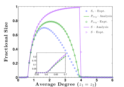
Figure 1: (Color online) The fractional size of the giant vulnerable cluster, $S_{v}$, the final cascade size $S$ and the triggering probability $P_{trig}$ are plotted for $n=5\times 10^{5}$, $\alpha=0.5$, $\tau$ is fixed at $\tau^{\star}=0.18$, and $\mathbb{F}$ and $\mathbb{W}$ are Erdös-Rényi networks with mean degrees $z_{1}$ and $z_{2}$, respectively. The content parameter is taken to be $(a)$ $c=0.25$ and $(b)$ $c=1$. The lines correspond to the analytical results obtained from Eqs. (8) and (13), whereas symbols represent experimental results averaged over $100$ independent realizations for $S_{v}$ and $S$, and over $5,000$ realizations for $P_{trig}$. (Insets) The same plots at a higher resolution on $z_{1}=z_{2}$ near the lower phase transition.

IV Numerical Results

We now illustrate our findings by numerical simulations. In our first example we consider $n=5\times 10^{5}$ nodes in the physical network $\mathbb{W}$ and assume that only half of these nodes are members of the network $\mathbb{F}$; i.e., we set $\alpha=0.5$. Following the references Watts (2002); Gleeson (2008); Brummitt et al. (2012); Payne and Eppstein (2009) we fix the thresholds at $\tau=\tau^{\star}=0.18$ and assume that both $\mathbb{F}$ and $\mathbb{W}$ are Erdös-Rényi networks Bollobás (2001) with mean degrees $z_{1}$ and $z_{2}$, respectively. Figure 1 shows the fractional size of the giant vulnerable cluster $S_{v}$, the triggering probability $P_{trig}$, and the expected cascade size $S$ w.r.t. $z_{1}=z_{2}$ for two different contents. For the first content $\mathcal{C}_{1}$ we assume that $c=0.25$, meaning that type-$2$ links are four times as important as type-$1$ links in spreading this content, and plot the corresponding results in Figure 1. For the second content $\mathcal{C}_{2}$, we assume that both types of links are equivalent w.r.t. spreading the content, i.e., $c=1$, and show the results in Figure 1. In all cases, lines correspond to our analysis results from Eqs. (8) and (13), whereas symbols are obtained from computer simulations: For each parameter set, we generated independent realizations of the graphs $\mathbb{F}$ and $\mathbb{W}$, and then observed the cascade process over the graph $\mathbb{H}$ upon activating an arbitrary node. The size $S_{v}$ of the giant vulnerable component is computed by finding the GSCC of the directed graph induced by the vulnerable nodes as described in Section III.1. The results are given by averaging over $100$ (resp. $5,000$) independent runs for $S_{v}$ and $S$ (resp. $P_{trig}$).

Figure 1 leads to a number of interesting observations. First, we see an excellent agreement between the analytical results and simulations, confirming the validity of our analysis; the discrepancy near the upper phase transition is due to finite size effect. Second, we see how content might impact the dynamics of complex contagions over the same network. For content $\mathcal{C}_{1}$ we see that global cascades are possible when $1.0\leq z_{1}=z_{2}\leq 4.9$, whereas $\mathcal{C}_{2}$ can spread globally only if $0.7\leq z_{1}=z_{2}\leq 3.9$. We also see that on the range where global cascades are possible for both contents (namely $1.0\leq z_{1}=z_{2}\leq 3.9$), the probability of them taking place can still differ significantly; e.g., if $z_{1}=z_{2}=3$, we have $P_{trig}=0.84$ for $\mathcal{C}_{1}$, while for $\mathcal{C}_{2}$ we have $P_{trig}=0.65$. Finally, simulations confirm the simultaneous appearance of the GSCC and GIN in the subgraph of vulnerable nodes in $\mathbb{H}$ as understood from the identical parameter ranges that give positive values for $S$, $P_{trig}$ and $S_{v}$; see also the Inset of Figure 1. Therefore, the possibility of observing global cascades without a giant vulnerable cluster is ruled out in our model, although this possibility exists in general.

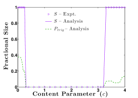
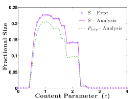
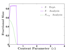
Figure 2: (Color online) We see the variation of cascade probability $P_{trig}$ and cascade size $S$ with respect to the content parameter $c$, when $\alpha=0.5$, $\tau=\tau^{\star}=0.18$, and $\mathbb{F}$ and $\mathbb{W}$ are Erdös-Rényi networks with mean degrees $z_{1}$ and $z_{2}$, respectively. We set $(a)$ $z_{1}=1.5$, $z_{2}=5.5$, $(b)$ $z_{1}=z_{2}=0.7$, $(c)$ $z_{1}=6.0$, $z_{2}=1.5$.

For a better demonstration of the effect of content on the probability and size of global cascades, we now consider a different experimental set-up. This time, for three different cases, we fix all the parameters except the content-parameter $c$, and observe the variation of $P_{trig}$ and $S$ with respect to $c$. The results are depicted in Figure 2. In all cases, we set $n=5\times 10^{5}$, $\alpha=0.5$, $\tau=\tau^{\star}=0.18$, and assume that $\mathbb{F}$ and $\mathbb{W}$ are Erdös-Rényi networks with mean degrees $z_{1}$ and $z_{2}$, respectively. In Figure 2, we consider the case $z_{1}=1.5$ and $z_{2}=5.5$, and see that global cascades are possible only for $0\leq c\leq 0.27$, and $c\geq 3.22$, but no global cascade can take place in the range $0.28\leq c\leq 3.21$. This can be explained as follows: When $c$ is too small, the spreading of the content is governed solely by network $\mathbb{W}$ (with average degree $z_{2}=5.5$), on which large global cascades are possible with very low probability; in other words network $\mathbb{W}$ is close to the upper phase transition threshold. As $c$ gets larger, the effect of $\mathbb{F}-$links becomes considerable, and the connectivity of the overall network (with respect to the spread of the current content) increases. This eventually causes global cascades to disappear due to the high local stability (i.e., connectivity) of the nodes. However, further increase in $c$ shifts the bias towards $\mathbb{F}-$links, and due to lower average degree in $\mathbb{F}$, this causes a decrease in the local stability of the nodes and brings global cascades back to the existence.

In Figure 2, we set $z_{1}=z_{2}=0.7$. This time, we see an exactly opposite dependence of cascade sizes on the parameter $c$. Namely, global cascades are not possible when $c$ is too small or too large, but they do take place in the interval $0.5\leq c\leq 2.5$. This is because, under the current setting, both networks $\mathbb{F}$ and $\mathbb{W}$ have limited connectivity, so that global cascades do not take place in either of the networks separately. Therefore, if $c$ is too small (resp. too large), only $\mathbb{W}$ (resp. $\mathbb{F}$) can spread the content and all triggering events have finite size as confirmed in the plot by the non-existence of global cascades for $c\leq 0.4$ and $c\geq 2.6$. But, for $c$ relatively close to unity, the two networks spread the content collaboratively, yielding a high enough connectivity in the overall network $\mathbb{H}$ to achieve a positive probability of global cascades.

The situation is somewhat different in the case of Figure 2, where we have $z_{1}=6.0$ and $z_{2}=1.5$: For contents that mainly spread over $\mathbb{W}$-links, i.e., for $c$ close to zero, global spreading events take place with positive probability since network $\mathbb{W}$ (with average degree $z_{2}=1.5$) satisfies the global spreading condition. However, as $c$ gets larger, the high average degree in network $\mathbb{F}$ (and, thus the high local stability of the nodes) makes it harder for the content to spread in the overall network $\mathbb{H}$, eventually causing the probability of global cascades drop to zero. This is confirmed in Figure 2 as we see that global cascades take place only for contents with $c\leq 0.5$ and any content with $c\geq 0.6$ dies-out before reaching a non-trivial fraction of the network.

We continue our simulation study by depicting the variation of the cascade window with respect to content parameter $c$ in Figure 3. We see that for each $\tau^{\star}$, the parameter $c$ changes the range of $z_{1}=z_{2}$ for which global cascades can occur in a non-trivial way. For instance, none of the three regions cover one another. In fact, the cascade window for $c=4$ is contained in that of $c=1$ for most of the $\tau^{\star}$ values, but, with $z_{1}=z_{2}=4$ and $\tau^{\star}$ in $(0.17,0.18)$ cascades do not occur for $c=1$ while they do for $c=4$. We also see that the content parameter $c$ can effect the maximum threshold $\tau^{\star}$ for which global cascades are possible. When $c=1$ and $c=0.1$, cascades can take place for $\tau^{\star}\leq 0.25$, whereas the upper-bound is reduced to $0.23$ for $c=4$.

Finally, we test our theory for networks which are not locally tree like. In fact, most real networks are known Serrano and Boguñá (2005) to exhibit a phenomenon often called clustering (or transitivity), informally defined as the propensity of a node’s neighbors to be neighbors as well. Since our theory is developed for networks that do not have clustering, we do not expect our results to provide good estimations for clustered networks; in the case of Watts’ threshold model, it is already shown Hackett et al. (2011) that clustering can have a significant impact on the size of global cascades. Nevertheless, we would like to provide the first step in showing the effect of clustering on content-dependent cascading processes in multiplex networks.

To this end, we generate random clustered networks $\mathbb{F}$ and $\mathbb{W}$ as prescribed by Newman Newman (2009) and Miller Miller (2009). Namely, we consider distributions $p_{st}^{f}$ and $p_{st}^{w}$ that give the probability of a node being connected to $s$ single edges and $t$ triangles; conventional degree distributions are then given by $p_{k}^{f}=\sum_{s,t}p_{st}^{f}\delta_{k,s+2t}$ and $p_{k}^{w}=\sum_{s,t}p_{st}^{w}\delta_{k,s+2t}$. For convenience, we consider a doubly Poisson distribution for $p_{st}$; namely, we set

$$p_{st}^{f}=e^{-z_{1}}\frac{z_{1}^{s}}{s!}\cdot e^{-z_{1}/2}\frac{(z_{1}/2)^{t}}{t!},\quad s,t=0,1,\ldots$$ (14)

and define $p_{st}^{w}$ similarly with $z_{1}$ replaced by $z_{2}$. Notice that average degrees are now given by $2z_{1}$ and $2z_{2}$ in networks $\mathbb{F}$ and $\mathbb{W}$, respectively. With $n=10^{5}$, $\alpha=0.5$, $\tau=\tau^{\star}=0.18$ and $c=0.5$, we show in Figure 3 the variation of the cascade size $S$ with respect to average degrees $2z_{1}=2z_{2}$. As before, the line corresponds to the analytical solution (obtained from Eq. (13)), whereas symbols are obtained from simulations by averaging over $50$ experiments for each point. Also, in the Inset of Figure 3, we plot the average clustering coefficient Newman (2009) observed for networks $\mathbb{W}$ and $\mathbb{F}$; with $z_{1}=z_{2}$ both networks have (statistically) identical clustering coefficients.

As expected, we do not see a good match between the predictions of our analysis (zero-clustering) and the actual cascade size from experiments (positive clustering). However, these results agree with the double faceted picture drawn in Hackett et al. (2011) for the effect of clustering on cascade sizes in Watts’ model: When average degrees are small, clustering decreases the expected size of global cascades, whereas after a certain value of average degree, clustering increases the expected cascade size.

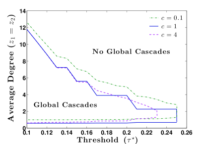
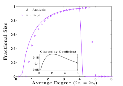
Figure 3: (Color online) (a) We see the cascade windows for several $c$ values when $\alpha=0.5$, $\tau=\tau^{\star}$, and $\mathbb{F}$ and $\mathbb{W}$ are Erdös-Rényi networks with mean degrees $z_{1}$ and $z_{2}$, respectively. In other words, the lines enclose the region of the $(\tau^{\star},z_{1}=z_{2})$ plane for which the global cascade condition $\sigma(\bm{J}_{p})>1$ is satisfied; outside the boundary, we have $\sigma(\bm{J}_{p})\leq 1$ and global cascades can not take place. (b) Global cascade size $S$ when $\mathbb{F}$ and $\mathbb{W}$ are random clustered networks with degree distributions given by (14). We take $n=10^{5}$, $\alpha=0.5$, $\tau=\tau^{\star}=0.18$ and $c=0.5$. The line corresponds to analytical prediction from (13), whereas symbols are obtained from simulations by averaging over 50 independent realizations. (Inset) Average clustering coefficient Newman (2009) versus $2z_{1}=2z_{2}$.

V Conclusion

We have determined the condition, probability and the size of global cascades in random networks with classified links. This is done under a new contagion model where nodes switch state when their perceived (content-dependent) proportion of active neighbors exceed a certain threshold. Our results highlight the effect of content and link classification in the characteristics of global cascades, and show how different content may have different spreading characteristics over the same network. Also, the results given here extend the existing work on complex contagions to multiple overlay networks whose vertices are not disjoint.

Our findings also contain some of the existing results as special cases. For instance, our results may be applied to a wide range of processes on the network $\mathbb{H}$ by appropriately selecting the neighborhood response function $F(\bm{m},\bm{k})$. In particular, the general results of Section III include the solutions for bond percolation, and simple contagion processes by setting $\rho_{\bm{k},1}=\rho_{\bm{k},2}=T$ for some transmissibility $T$ in $[0,1]$. The threshold model of Watts Watts (2002) is also covered by our theory by setting the content parameter $c$ to unity in all cases.

We believe that the results presented here give some interesting insights into the cascade processes in complex networks. In particular, our results might help better understand such processes and may lead to more efficient control of them. Controlling cascade processes is particularly relevant when dealing with cascading failures in interdependent structures as well as when marketing a certain consumer product. Finally, the formulation presented here opens many new questions in the field. For instance, the dynamics of cascade processes are yet to be investigated on clustered or degree-correlated networks under the content-dependent threshold model introduced here. Another challenging problem would be to formalize the results given in this paper without using a mean-field approach; in fact, very recently Lelarge and co-workers Lelarge (2012); Coupechoux and Lelarge (2012) have obtained rigorous results for the condition and size of global cascades in Watts’ threshold model.

References

- Watts (2002) D. J. Watts, Proceedings of the National Academy of Sciences 99, 5766 (2002).
- Dodds and Watts (2004) P. Dodds and D. J. Watts, Phys. Rev. Lett. 92, 218701 (2004).
- Duan et al. (2005) W. Duan, Z. Chen, Z. Liu, and W. Jin, Phys. Rev. E 72, 026133 (2005).
- Murray (2002) J. D. Murray, Mathematical Biology, 3rd ed. (Springer, New York (NY), 2002).
- Anderson and May (1991) R. M. Anderson and R. M. May, Infectious Diseases of Humans (Oxford University Press, Oxford (UK), 1991).
- Buldyrev et al. (2010) S. V. Buldyrev, R. Parshani, G. Paul, H. E. Stanley, and S. Havlin, Nature 464, 1025 (2010).
- Buldyrev et al. (2011) S. V. Buldyrev, N. W. Shere, and G. A. Cwilich, Phys. Rev. E 83, 016112 (2011).
- Cho et al. (2010) W. Cho, K. I. Goh, and I. M. Kim, arXiv:1010.4971v1 [physics.data-an] (2010), 1010.4971v1 .
- Cohen and Havlin (2010) R. Cohen and S. Havlin, Complex Networks: Structure, Robustness and Function (Cambridge University Press, United Kingdom, 2010).
- Huang et al. (2011) X. Huang, J. Gao, S. Buldyrev, S. Havlin, and H. E. Stanley, Phys. Rev. E 83 (2011).
- Shao et al. (2011) J. Shao, S. Buldyrev, S. Havlin, and H. E. Stanley, Phys. Rev. E 83, 036116 (2011).
- Vespignani (2010) A. Vespignani, Nature 464, 984 (2010).
- Yağan et al. (2012) O. Yağan, D. Qian, J. Zhang, and D. Cochran, “Optimal allocation of interconnecting links in cyber-physical systems: Interdependence, cascading failures and robustness,” (2012), to appear in the Special Issue of IEEE Transactions on Parallel and Distributed Systems on Cyber-Physical Networks. Doi:10.1109/TPDS.2012.62. Also available online at arXiv:1201.2698v2.
- Yağan et al. (2011a) O. Yağan, D. Qian, J. Zhang, and D. Cochran, in Proc. of the Third International Workshop on Network Science for Communication Networks (NetSciCom) (2011).
- Granovetter (1978) M. Granovetter, The American Journal of Sociology 83, pp. 1420 (1978).
- Newman et al. (2002) M. E. J. Newman, S. Forrest, and J. Balthrop, Phys. Rev. E 66 (2002), 10.1103/PhysRevE.66.035101.
- Balthrop et al. (2004) J. Balthrop, S. Forrest, M. E. J. Newman, and M. W. Williamson, Science 304, 527 (2004).
- Schelling (1973) T. C. Schelling, The Journal of Conflict Resolution 17, pp. 381 (1973).
- Tang et al. (2011) S. Tang, J. Yuan, X. Mao, X.-Y. Li, W. Chen, and G. Dai, in Proceedings of IEEE INFOCOM 2011 (2011) pp. 2291 –2299.
- Spafford (1991) E. H. Spafford, The Internet Worm Incident, Tech. Rep. CSD-TR-933 (Purdue University, Dept. of Comp. Sci., 1991).
- Padgett and Ansell (1993) J. F. Padgett and C. K. Ansell, American Journal of Sociology 98, 1259 (1993).
- Szell et al. (2010) M. Szell, R. Lambiotte, and S. Thurner, Proceedings of the National Academy of Sciences 107, 13636 (2010).
- Lee et al. (2012) K.-M. Lee, J. Y. Kim, W. Cho, K.-I. Goh, and I. M. Kim, New J. Phys. 14 (2012).
- Brummitt et al. (2012) C. D. Brummitt, K.-M. Lee, and K.-I. Goh, Phys. Rev. E 85, 045102(R) (2012).
- Note (1) The notion of perceived proportion of active neighbors was first suggested by Granovetter (Granovetter, 1978, pp. 1429) as a way of taking the social structure into account in the study of cascading processes. There, he suggested, as an example, that the influence of friends would be twice that of strangers in a fully mixed population; in the formulation (1), this amounts to setting (with ) and , where links of type- are considered as friendship links, whereas links of type- are considered as links with strangers.
- Newman et al. (2001) M. E. J. Newman, S. H. Strogatz, and D. J. Watts, Phys. Rev. E 64, 026118 (2001).
- Yağan et al. (2011b) O. Yağan, D. Qian, J. Zhang, and D. Cochran, “Conjoining speeds up information diffusion in overlaying social-physical networks,” (2011b), submitted. Available online at arXiv:1112.4002v1 [cs.SI].
- Gleeson (2008) J. P. Gleeson, Phys. Rev. E 77, 046117 (2008).
- Dodds and Payne (2009) P. S. Dodds and J. L. Payne, Phys. Rev. E 79 (2009).
- Payne et al. (2011) J. L. Payne, K. D. Harris, and P. S. Dodds, Phys. Rev. E 84, 016110 (2011).
- Melnik et al. (2011) S. Melnik, J. A. Ward, J. P. Gleeson, and M. A. Porter, Arxiv (2011), 1111.1596v1 .
- Note (2) We remind that these definitions are given merely for illustration purposes and do not effect our technical results. Our intuition is to distinguish people with close relationships (as understood from their engagement in two-way communications) and those that are merely Facebook friends who receive information and status updates from one another but never talk to each other. Recent statistics show that Marlow et al. (2009), on average, a user with friends in Facebook engages in a mutual communication with only of them; a number likely to represent one’s close relationships. Also, we refer to the network as a physical one since its links appear between people that have close relationships. For instance, we regard a mother using Facebook to communicate with her daughter (who lives abroad) as if they belong to each other’s physical network.
- Bollobás (2001) B. Bollobás, Random Graphs (Cambridge Studies in Advanced Mathematics, Cambridge University Press, Cambridge (UK), 2001).
- Molloy and Reed (1995) M. Molloy and B. Reed, Random Structures and Algorithms 6, 161 (1995).
- Söderberg (2003a) B. Söderberg, Phys. Rev. E 68, 015102 (2003a).
- Söderberg (2003b) B. Söderberg, Acta Phys. Pol. B 34, 5085 (2003b).
- Newman (2002) M. E. J. Newman, Phys. Rev. E 66 (2002).
- Hackett et al. (2011) A. Hackett, S. Melnik, and J. P. Gleeson, Phys. Rev. E 83, 056107 (2011).
- Dorogovtsev et al. (2001) S. N. Dorogovtsev, J. F. F. Mendes, and A. N. Samukhin, Phys. Rev. E 64 (2001), 10.1103/PhysRevE.64.025101.
- Boguñá and Serrano (2005) M. Boguñá and M. Á. Serrano, Phys. Rev. E 72, 016106 (2005).
- Note (3) Consider a network on vertices with edges where refers to an edge directed from to . In the limit , a positive fraction of nodes have infinite in- and out-components, but the network has no strongly connected component since for each node, its in-component and out-component are disjoint.
- Dousse (2012) O. Dousse, in Proceedings of IEEE International Symposium on Information Theory (ISIT) (2012).
- Söderberg (2003c) B. Söderberg, Phys. Rev. E 68, 026107 (2003c).
- Gleeson and Cahalane (2007) J. P. Gleeson and D. J. Cahalane, Phys. Rev. E 75, 056103 (2007).
- Sethna et al. (1993) J. Sethna, K. Dahmen, S. Kartha, J. A. Krumhansl, B. W. Roberts, and J. D. Shore, Phys. Rev. Lett. 70, 3347 (1993).
- Payne and Eppstein (2009) J. L. Payne and P. D. M. J. Eppstein, Phys. Rev. E 80, 026125 (2009).
- Serrano and Boguñá (2005) M. Á. Serrano and M. Boguñá, Phys. Rev. E 72, 036133 (2005).
- Newman (2009) M. E. J. Newman, Phys. Rev. Lett. 103, 058701 (2009).
- Miller (2009) J. C. Miller, Physical Review E 80, 020901 (2009).
- Note (4) Simple contagions are defined as diffusion processes where nodes become infected (or active) after only one incident of contact with an infected neighbor. Examples include spread of diseases and information.
- Lelarge (2012) M. Lelarge, Games and Economic Behavior 75, 752 (2012).
- Coupechoux and Lelarge (2012) E. Coupechoux and M. Lelarge, Arxiv (2012), 1202.4974v1 .
- Marlow et al. (2009) C. Marlow, L. Byron, T. Lento, and I. Rosenn, Online at http://overstated.net/2009/03/09/maintained-relationships-on-facebook (2009).