Red Supergiant Stars as Cosmic Abundance Probes:
NLTE Effects in J-band Iron and Titanium Lines

Abstract

Detailed non-LTE calculations for red supergiant stars are presented to investigate the influence of NLTE on the formation of atomic iron and titanium lines in the J-band. With their enormous brightness at J-band red supergiant stars are ideal probes of cosmic abundances. Recent LTE studies have found that metallicities accurate to 0.15 dex can be determined from medium resolution spectroscopy of individual red supergiants in galaxies as distant as 10 Mpc. The non-LTE results obtained in this investigation support these findings. Non-LTE abundance corrections for iron are smaller than 0.05 dex for effective temperatures between 3400K to 4200K and 0.1 dex at 4400K. For titanium the non-LTE abundance corrections vary smoothly between -0.4 dex and +0.2 dex as a function of effective temperature. For both elements, the corrections also depend on stellar gravity and metallicity. The physical reasons behind the non-LTE corrections and the consequences for extragalactic J-band abundance studies are discussed.

1 Introduction

One of the most promising ways to constrain the theory of galaxy formation and evolution in a dark energy and cold dark matter dominated universe is the determination of the chemical composition of star forming galaxies in the nearby and high redshift universe. The observations of the relationship between central metallicity and galactic mass (Lequeux et al., 1979; Tremonti et al., 2004; Maiolino et al., 2008) and of metallicity gradients in spiral galaxies (Garnett et al., 1997; Skillman, 1998; Garnett, 2004) are intriguing and a clear challenge of the theory, which uses these observations to test the theoretical predictions of hierarchical clustering, galaxy formation, merging, infall, galactic winds and variability of star formation activity and IMF (Prantzos & Boissier, 2000; Naab & Ostriker, 2006; Colavitti et al., 2008; Yin et al., 2009; Sánchez-Blázquez et al., 2009; De Lucia et al., 2004; de Rossi et al., 2007; Finlator & Davé, 2008; Brooks et al., 2007; Köppen et al., 2007; Wiersma et al., 2009; Davé et al., 2011a, b).

So far most of our information about the metal content of star forming galaxies is obtained from a simplified analysis of H II region emission lines, which use the fluxes of the strongest forbidden lines of (most commonly) [O II] and [O III] relative to H_β. This approach is very powerful and appealing, since these emission line can be observed in galaxies through the whole universe from low to high redshift. However, it has two weaknesses. First, this approach yields basically only the oxygen abundance, which is then taken, in the absence of any other information, as a place holder for metallicity. Secondly, the abundances depend heavily on the calibration of the strong line method (Kewley & Ellison, 2008) and are therefore subject to systematic uncertainties of up to $0.8$ dex (Kudritzki et al., 2008; Bresolin et al., 2009).

An alternative approach avoiding these weaknesses is the spectroscopic analysis of individual supergiant stars. Here, much progress has been made through the non-LTE low resolution optical spectroscopy of BA blue supergiants (see e.g. Kudritzki et al., 2008; Kudritzki, 2010; Kudritzki et al., 2012, for application to spiral galaxies in the Local group). However, this technique is restricted to spectroscopy in the optical. In consequence, it will not be able to take advantage of the fact that the next generation of extremely large telescopes such as the GMT, TMT, and the E-ELT will be diffraction limited telescopes at IR wavelengths allowing for adaptive optics (AO) supported multi-object spectroscopy.

In this sense, the use of red supergiants (RSGs) as extragalactic abundance probes has a much larger potential. As direct successors of blue supergiants they have the same masses (8 to 40 $M_{\odot}$ at the main sequence) and the same enormous luminosities (10⁵ to 10⁶ L/L${\odot}$), but their SEDs peak in the infrared, where the gain in limiting magnitude through AO goes with the fourth power of telescope diameter. Recently, Davies et al. (2010) (hereinafter DKF10) have introduced a novel technique, which uses medium resolution (R $\approx$ 3000) spectroscopy in the J-band to derive stellar parameters of RSGs with the accuracy of $\sim$ 0.15 dex per individual star. The J-band spectra of of RSGs are dominated by strong and isolated atomic lines of iron, titanium, silicon and magnesium, while the molecular lines of OH, H₂O, CN, and CO which plague the H- and K-bands are weak and appear as a pseudo-continuum at R $\sim 3000$ resolution. The prospects of the J-band technique in application to RSGs were discussed by Evans et al. (2011), who showed that with future instruments it would be possible to measure abundances of various chemical elements out to enormous distances of 70 Mpc.

In the view of these perspectives, it is important to investigate the DKF10 method in more detail. One crucial question is how model atmosphere and line formation calculations are affected by the departures from Local Thermodynamic Equilibrium (LTE), which are expected because of extremely low gravities and hence low densities of RSG atmospheres. Detailed non-LTE line formation calculations for RSGs focussing on the key diagnostic lines in the J-band are, thus, a first step. In this paper, we present the first calculations of this type and investigate the formation of iron and titanium lines and the influence of non-LTE effects on the determination of abundances in the J-band. In future work, we plan to extend these studies to the formation of silicon and magnesium lines, which are important for the determination of effective temperature in the DKF10 method.

The paper is structured as follows. In sections 2 and 3 we describe the model atmospheres and the details of the line formation calculations. Section 4 presents the results: departure coefficients, line profiles and equivalent widths in LTE and non-LTE and non-LTE abundance corrections for chemical abundance studies. Section 5 discusses the consequences for the new J-band diagnostic technique and aspects of future work.

2 Model Atmospheres

The atmospheric structure for our non-LTE line formation calculations is provided by the MARCS model atmospheres. The physical assumptions underlying these atmospheres are described in Gustafsson et al. (2008). In short, these LTE models are spherically-symmetric, in 1D hydrostatic equilibrium and include convection within the framework of the mixing-length theory. A careful discussion of the strengths and the weaknesses of these models is given by Gustafsson et al. (2008); Plez (2010). The reference solar abundance mixture in these models is that of Grevesse et al. (2007).

For our investigation we use a small grid of models computed assuming the mass of 15 $M_{\odot}$with five effective temperatures (T_eff = 3400, 3800, 4000, 4200, 4400K), three gravities ($\log g=1.0$, $0.0$, $-0.5$ (cgs)), three metallicities ([Z]$\,\equiv\,$ log Z/Z_⊙ $=-0.5$, $0.0$, $+0.5$). We also use two values of micro-turbulence $\xi_{t}=2$ and 5 km/s, respectively. This grid covers the range of atmospheric parameters expected for RSGs (see DKF10). We also compared the 1 and 15 $M_{\odot}$models for the same parameters finding very small differences in the NLTE abundance corrections.

For the current analysis, the model atmospheres were carefully extrapolated to a continuum optical depth at $500$ nm $\log\tau_{\rm 500}=-5$, since for certain combinations of RSG atmospheric parameters the cores of the Ti and Fe lines have contributions from atmospheric layers around optical depth $\log\tau_{\rm 500}\sim-3.5$, which is close to the top boundary of the MARCS atmospheric models ($\log\tau_{\rm 500}=-4.0$). By this extrapolation we explored whether higher layers could contribute to the formation of the IR lines investigated. No significant effects were found.

At the highest effective temperature (T_eff = 4400K) and lowest gravity ($\log g=-0.5$) the MARCS models show a very slight temperature inversion, although they are converged. The locations of these inversions can be noticed from the kinks in the plots of departure coefficients (Fig. 5 and 7, see Sect. 3.1 and 3.2) for Fe iand Ti i. They do not have any significant effects on the results.

3 Non-LTE Line Formation

3.1 Statistical equilibrium calculations

For the non-LTE line formation calculations we use DETAIL, a non-LTE code widely used for hot stars (Przybilla et al., 2006) as well as for cool stars (Butler & Giddings, 1985). DETAIL is a well established and well tested code, which is fast and very efficient through the use of the accelerated lambda iteration scheme in the formulation of Rybicki & Hummer (1991, 1992), and allows for the self-consistent treatment of overlapping transitions and continua. It is worth noting that DETAIL requires the partial pressures of all atoms and important molecules to be supplied with a model atmosphere; these were computed using the MARCS equation-of-state package.

Since the non-LTE effects depend crucially on the radiation field at all wavelengths, it is important that all relevant opacities are included in the statistical equilibrium calculations. The background line opacity is computed directly for each wavelength in the model atom using extensive linelists extracted from the NIST (Ralchenko et al., 2012) and Kurucz databases. For the current project, these tables were complemented by the TiO line data of Plez (1998) to account for the extreme line blanketing by TiO molecules. A comparison of spectral energy distributions calculated with DETAIL and MARCS for two typical RSG models is given in Fig. 1. The agreement is satisfactory.

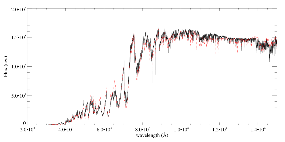
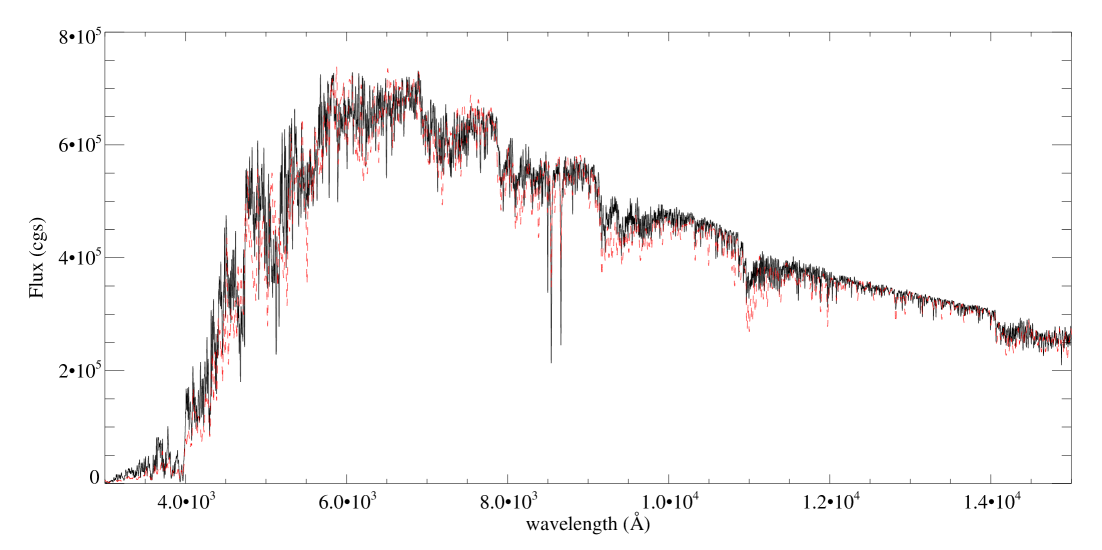
Figure 1: Emergent fluxes computed with DETAIL (black solid) as compared with the original SED’s from MARCS (red, dashed). Top: $T_{\rm eff}=3400$ K, $\log g=0$, [Z] $=0$. Bottom: $T_{\rm eff}=4400$ K, $\log g=0$, [Z] $=0$.

The non-LTE radiative transfer in DETAIL is done in plane-parallel geometry. This might be a reason of concern, since the atmospheres of RSGs have a large scale height because of small $\log g$. Heiter & Eriksson (2006) have used the spherically extended MARCS models to compare LTE line formation calculations with radiative transfer in spherically extended geometry with the calculations done with the plane-parallel approximation. At most extreme cases abundance corrections were smaller than $0.1$ dex indicating that the combination of spherically extended models with plane parallel radiative transfer yields reasonable results. We note that the lowest gravities used by Heiter & Eriksson (2006) were $\log g=0.5$ (cgs), whereas the lowest gravities in our grid are a factor of ten lower, i.e. $\log g=-0.5$ (see below). On the other hand, Heiter & Eriksson (2006) investigated the most extreme models with very low stellar mass, i.e. 1 $M_{\odot}$. However, since the spherical extend of a line forming atmosphere $\Delta$R in units of the photospheric radius R is:

$$\Delta R/R\sim T_{\rm eff}/(g~{}M)^{1/2}$$ (1)

and RSGs are massive stars with masses equal and larger than 10 $M_{\odot}$, we expect the effects of sphericity to be small. Indeed, compared with Heiter & Eriksson’s largest extension of 12%, $\Delta$R/R of our most extreme model (calculated with 15 $M_{\odot}$) is 7%. We note however that most likely real RSG atmospheres are more extended due to hydrodynamical phenomena (Chiavassa et al., 2011, and references therein). We have also checked $\Delta$R/R for the line forming region of the IR lines of our investigation and found values less then $2$ %. This, in addition to a relatively small geometrical dilution factor of the radiation field ($(1/1.07)^{2}$ or 14% in the most extreme model with $\Delta$R/R = 7%), leads us to conclude that the NLTE abundance corrections are likely very similar in plane-parallel and spherical geometry.

The line profiles and the NLTE abundance corrections were computed with a separate code SIU (Reetz, 1999) using the level departure coefficients from DETAIL. SIU and DETAIL share the same physics and line lists.

3.2 Model atoms

The atomic models for Ti and Fe are essentially those described in Bergemann (2011) and Bergemann et al. (2012), however some modifications were implemented for the current analysis. The models include the first two ionization stages of each element accounting for $332$ and $397$ levels of Ti and Fe, respectively. For Fe i  we have added the fine structure splitting of the $a\,^{5}{\rm P}$ and $z\,^{5}{\rm D}^{{\rm\circ}}$ states, since the J-band IR lines of our investigation form between these levels. We also removed a number of theoretically-predicted Fe i levels and radiative transitions, which according to our tests are not important for the statistical equilibrium of the element in RSG atmospheres. The Fe level diagram with transition related to the J-band lines investigated here is shown in Fig. 2. Similarly, the Ti i model was extended by the fine structure of all levels below $2.73$ eV, and all transitions involving these levels were updated (Fig. 2). The number of radiatively-allowed transitions is, thus, $4943$ and $5328$ for Ti and Fe, respectively; the gf-values of these transitions were taken from various sources (Bergemann, 2011; Bergemann et al., 2012). Photoionization cross-sections for Fe i were kindly provided by Bautista (2011, private communication); they are computed on a more accurate energy mesh and provide better resolution of photoionization resonances compared to the older data, e.g. provided in the TOPbase. For Ti the hydrogenic approximation was adopted.

To compute collisional rates, we relied on standard recipes, commonly used in NLTE calculations for late-type stars, as no better alternatives are available. Electron impact excitation and ionization cross-sections were computed using the semi-empirical formulae from Seaton (1962), van Regemorter (1962), and Allen (1973). Inelastic collisions with H i atoms were computed according to the Drawin’s formula in the formulation of Steenbock & Holweger (1984). From detailed comparison with more accurate quantum-mechanical and experimental data for other atoms, the recipes for e^- collisions are expected to give an order of magnitude accuracy (Mashonkina, 1996; Lind et al., 2011), whereas the situation with H i collisions is more uncertain. Recent quantum-mechanical calculations suggest that for bound-bound transitions the latter are exaggerated (Barklem et al., 2011, 2012), whereas charge transfer processes can not be described by the Drawin’s formulae at all. We note, however, that only light atoms, Li, O, Na, and Mg, have been investigated so far.

Here, we performed a set of test calculations varying the collision cross-sections by several orders of magnitude. As expected, the most influential factor is inelastic H i collisions, which is also well-known from the NLTE analysis of late-type stars (Gehren et al. 2001, Bergemann et a. 2012). However, even a factor of ten variation of these cross-sections leads to a change in the NLTE corrections for the IR Ti i lines by less than $0.07$ dex across the RSG parameter space. A notable effect on the coolest models (3400 - 3800 K) is seen when the bound-bound H i collision rates are decreased by four orders of magnitude. In this case, the NLTE corrections double. For the Fe i IR lines, the effect of varying the H i collisions is very small, on average of the order $0.03$ dex. In our recent work on low-mass FGK stars (Bergemann et al., 2012), we constrained the efficiency of inelastic H i collisions empirically, from the analysis of stars with parameters determined by independent methods. We can not follow the same approach in this work, as the sample of nearby RSG’s is very limited and stellar parameters are not accurate enough to permit calibration of collision efficiency using high-resolution spectra. A more accurate and realistic quantification of the uncertainties related to the collision rates will therefore have to await for detailed theoretical calculations and high-quality observations of RSG’s.

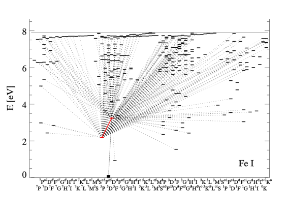
Figure 2: The Fe i non-LTE atomic model. The terms leading to the J-band IR transitions discussed are highlighted in red. Only radiative transitions to and from these levels are shown in this plot. The calculations use a much more complex model of Fe i with many more transitions and simultaneously also a detailed atomic model of Fe ii  which is also not shown here.

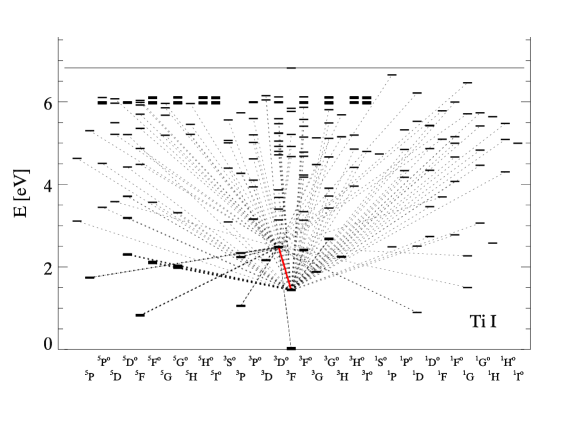
Figure 3: The Ti i non-LTE atomic model. The terms leading to the J-band IR transitions discussed are highlighted in red. Only radiative transitions to and from these levels are shown in this plot. The calculations use a much more complex model of Ti i with many more transitions and simultaneously also a detailed atomic model of Ti ii, which is not shown here.

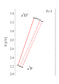
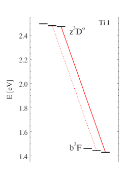
Figure 4: Fine structure splitting of Fe i (left) and Ti i (right) IR J-band lines.

4 Results

The NLTE effects will be discussed using the concept of level departure coefficients $b_{i}$

$$b_{i}=n_{i}^{\rm NLTE}/n_{i}^{\rm LTE}$$ (2)

where $n_{i}^{\rm NLTE}$ and $n_{i}^{\rm LTE}$ are NLTE and LTE atomic level populations [cm^-3], respectively.

Furthermore, the importance of the NLTE effects for the determination of element abundances can be assessed by introducing NLTE abundance corrections $\Delta_{\rm Fe,Ti}$, where:

$$\Delta_{\rm Fe,Ti}=\log\rm{A(Fe,Ti)}_{\rm NLTE}-\log\rm{A(Fe,Ti)}_{\rm LTE}$$ (3)

is the the logarithmic correction, which has to be applied to an LTE iron or titanium abundance determination A of a specific line to obtain the correct value corresponding to the use of NLTE line formation. We calculate these corrections at each point of our model grid for each line by matching the NLTE equivalent width through varying the Fe abundance in the LTE calculations. Note that from the definition of $\Delta_{\rm Fe,Ti}$ a NLTE abundance correction is positive, when for the same element abundance the NLTE line equivalent width is smaller than the LTE one, because it requires a lower LTE abundance to fit the NLTE equivalent width.

It shall be kept in mind that both Ti i and Fe i have a very complex atomic structure. For each of the energy levels, there are about a thousand of radiative and collisional processes, which contribute to the net population or de-population of a level. As a result, there is a strong interlocking of radiation field in different lines and continua, and it becomes highly non-trivial to isolate the processes explaining the populations of individual atomic levels once the statistical equilibrium has been established.

Thus, in the next two subsections (4.1 and 4.2), we will give only a qualitative and rather general description of the processes driving departures from LTE in the excitation-ionization equilibria of Ti and Fe, focusing mainly on the levels and transitions used in the spectroscopic J-band analysis of the RSG stars. The selected lines are given in the Table 1. Their wavelengths, excitation energies, and transition probabilities were extracted from the VALD database (Piskunov et al., 1995; Ryabchikova et al., 1997; Kupka et al., 1999, 2000). For the Fe i lines, the transition probabilities are taken from O’Brian et al. (1991). Under typical physical conditions in the RSG models, all these lines are relatively strong, with equivalent widths $W_{\lambda}$ exceeding few hundred mÅ.

4.1 Statistical equilibrium of Fe

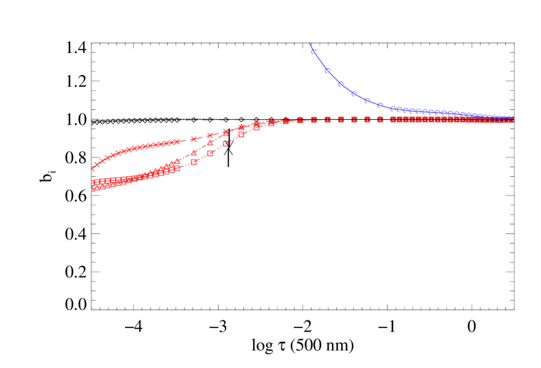
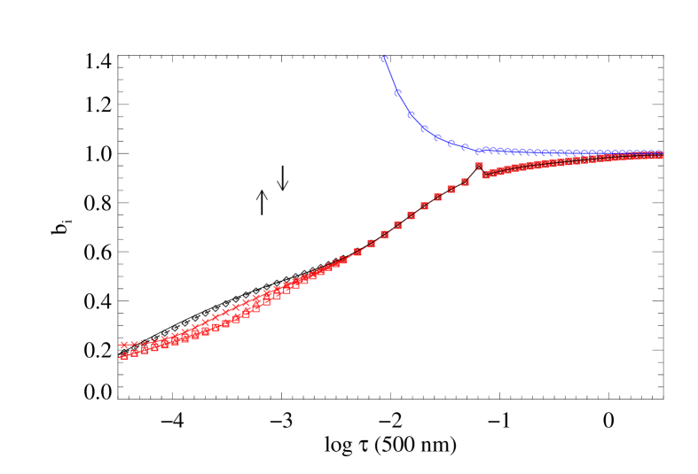
Figure 5: The NLTE departure coefficients of Fe i for RSG models with log g = -0.5, [Z] = -0.5 and T_eff = 3400K (top) and 4400K (bottom) as a function of optical depth. Blue: Fe ii ground state $a\,^{6}{\rm D}_{\rm 9/2}$. Black: lower fine structure levels of J-band IR transitions, $a\,^{5}{\rm P}_{\rm 1}$ (diamonds, dashed), $a\,^{5}{\rm P}_{\rm 2}$ (dotted), $a\,^{5}{\rm P}_{\rm 3}$ (solid). Red: upper fine structure levels of IR-transitions, $z\,^{5}{\rm D}^{{\rm\circ}}_{\rm 0}$ (crosses), $z\,^{5}{\rm D}^{{\rm\circ}}_{\rm 3}$ (squares, dashed), $z\,^{5}{\rm D}^{{\rm\circ}}_{\rm 4}$ (triangles). The LTE and NLTE line core optical depths $\log\tau(11973$ Å, Fe i$)=0$ are also indicated by the upward and downward directed arrows, respectively.

Statistical equilibrium of Fe in stellar atmospheres has been extensively studied in application to solar-type stars, i.e., FGK spectral types (Gehren et al. 2001,Mashonkina et al. 2011,Bergemann et al. 2012,Lind et al. 2012). However, all theses studies focused on the NLTE line formation of Fe i and Fe ii in the near-UV and optical spectral windows. Here we model the four near-IR Fe i transitions in the multiplet $296$ (Table 1), which connect the lowest metastable $2.2$ eV $a\,^{5}{\rm P}$ levels to the $3.2$ eV $z\,^{5}{\rm D}^{{\rm\circ}}$ levels. The departure coefficients for these selected Fe i levels are shown in Fig. 5 for two selected RSG models. The LTE and NLTE unity optical depths in the transition at $11973$ Å ($a\,^{5}{\rm P}_{\rm 3}$ $\leftrightarrow$ $z\,^{5}{\rm D}^{{\rm\circ}}_{\rm 4}$) are indicated by the upward and downward directed arrows, respectively.

In the atmospheres of the solar-type stars, the main NLTE effect on the Fe i number densities is over-ionization by super-thermal UV radiation field, which reduces the Fe i number densities compared to LTE. This effect is equally important for other minority atoms, such as Ti i  which constitute only a tiny fraction of the total element abundance. For example, everywhere in the solar photosphere, the ratio of total number densities of neutral to ionized iron, $N_{\rm FeI}/N_{\rm FeII}$, is always below $0.1$.

The situation is somewhat different in the cool atmospheres of RSGs. At T_eff = 3400K the ratio $N_{\rm FeI}/N_{\rm FeII}$ is about 10² at optical depths $\log\tau_{\rm 500}\leq-0.5$. In consequence, photoionization becomes utterly unimportant for the statistical equilibrium of neutral iron at this low temperature. For T_eff = 4400K $N_{\rm FeI}/N_{\rm FeII}$ varies between $0.01$ and $3.0$ depending on optical depth, metallicity and gravity. Here, photoionization can have an effect, although the radiative rates are generally small due to the low $T_{\rm eff}$ of the models in combination with the extreme line blanketing (recall that the metallicities are close to solar).

The analysis of the Fe i transition rates showed that for all models with $T_{\rm eff}=3400$ to $3800$ K, irrespective of their $\log g$ and [Fe/H], collisions fully dominate over radiatively-induced transitions out to the depths $\log\tau_{\rm 500}\sim-3$ (Fig. 5, top panel). Only near the outer boundary, $\log\tau_{\rm 500}\leq-3$, the departure coefficients of the upper level of the multiplet $296$, $z\,^{5}{\rm D}^{{\rm\circ}}$, deviate from unity, whereas the lower level $a\,^{5}{\rm P}$ retains its LTE populations all over the optical depth scale. As a result, deviations from LTE in the opacity of the Fe i lines are negligible, and the NLTE and LTE line formation depths nearly coincide (as shown by the vertical marks in Fig. 5). Very small NLTE effects, which show up in the line cores, are entirely due to the deviation of the line source function $S_{\rm ij}$ from the Planck function $B_{\nu}(T_{\rm e})$. Since $S_{\rm ij}/B_{\nu}(T_{\rm e})\sim b_{j}/b_{i}<1$, that is driven by the photon escape in the line wings, the line cores are slightly darker under NLTE and the NLTE abundance corrections $\Delta_{\rm Fe}$ are negative (Table 2 and 3). Metallicity and surface gravity have very small influence on the magnitude of NLTE effects for these cool models.

Larger departures from LTE are found for the hottest models with $T_{\rm eff}$ = 4400K (Fig. 5, bottom panel). They are caused by radiative pumping from the lower $a\,^{5}{\rm P}$ term to higher levels and strong collisional coupling. As a result $a\,^{5}{\rm P}$ becomes progressively more underpopulated in the inner atmospheric layers and the line absorption coefficient is reduced. At the same time collisional coupling induces $b_{i}\sim b_{j}$ and the line source function remains at the LTE value. As a consequence, the NLTE profiles become brighter in the core than the LTE profiles and the NLTE equivalent widths are smaller in NLTE. The magnitude of the NLTE effects decreases with increasing gravity and metallicity. The most extreme effects are found at $T_{\rm eff}=4400$ K, $\log g=-0.5$, and [Fe/H] $=-0.5$. NLTE and LTE line profiles for these parameters and for the model atmosphere with $T_{\rm eff}=4400$ K, $\log g=-0.5$, and [Fe/H] $=0.5$, are shown in Fig. 6. The value of the micro-turbulence has almost no influence on the size of the NLTE effects.

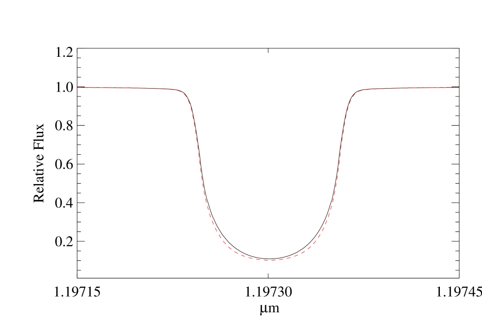
Figure 6: The NLTE (black, solid) and LTE (red, dashed) profiles of the Fe I line at $11973$ Å computed for T_eff = 4400K, log g = -0.5 and [Z] = -0.5 with microturbulence $\xi_{\rm t}=5$ km/s.

4.2 Statistical equilibrium of Ti

For Ti i, our calculations show that non-LTE effects are more significant than those for Fe i discussed in the previous section. The atomic structure of Ti i (ground state electronic configuration $1s^{2}2s^{2}2p^{6}3s^{2}3p^{6}3d^{2}4s^{2}$) is simpler than that of Fe i . In the NLTE model of Fe i , a very large number of levels allow for a more efficient collisional and radiative coupling, generally leading to a stronger overall thermalization of the level populations. We also note that the ionization potential of Ti i is only $6.82$ eV ($1.1$ eV lower than that of Fe i), thus the ionization balance is such that Ti ii is the dominant ionization stage for all models in our grid. The ratio of $N_{\rm TiI}/N_{\rm TiII}$ is 10^-2 to 10^-3 for the 4400K models and $0.1$ to 1 for the 3400K models.

The departure coefficients for the $b\,^{3}{\rm F}$ and $z\,^{3}{\rm D}^{{\rm\circ}}$ levels are shown in the Fig. 7. These levels with excitation energies of $1.43$ respectively $2.47$ eV give rise to the diagnostic IR Ti i transitions (Table 1). The Ti i NLTE effects are a strong function of effective temperature. At T_eff = 3400K the lower (metastable) $b\,^{3}{\rm F}$ states are overpopulated in the region of line formation through radiative transitions from higher levels and the upper levels $z\,^{3}{\rm D}^{{\rm\circ}}$ are depleted by radiative transitions to lower levels, in particular to the ground state. In consequence, the Ti i J-band absorption lines become stronger in NLTE compared to LTE because of the enhanced line absorption coefficient and the sub-thermal source function (see Fig. 8).

The situation changes towards higher effective temperatures. At T_eff = 4400K the radiation field has become powerful enough to deplete the lower $b\,^{3}{\rm F}$ states through radiative pumping into higher levels. While the upper $z\,^{3}{\rm D}^{{\rm\circ}}$ are populated from below in this way, they are also de-populated by radiative pumping to even higher levels, which leads to a net underpopulation. The strong de-population of the lower levels weakens the line absorption coefficient, while the source function remains close to the LTE value. As a result, the Ti i absorption lines become weaker in NLTE at higher temperatures (see Fig. 8).

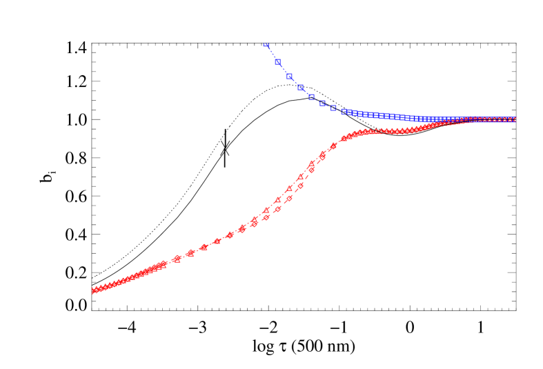
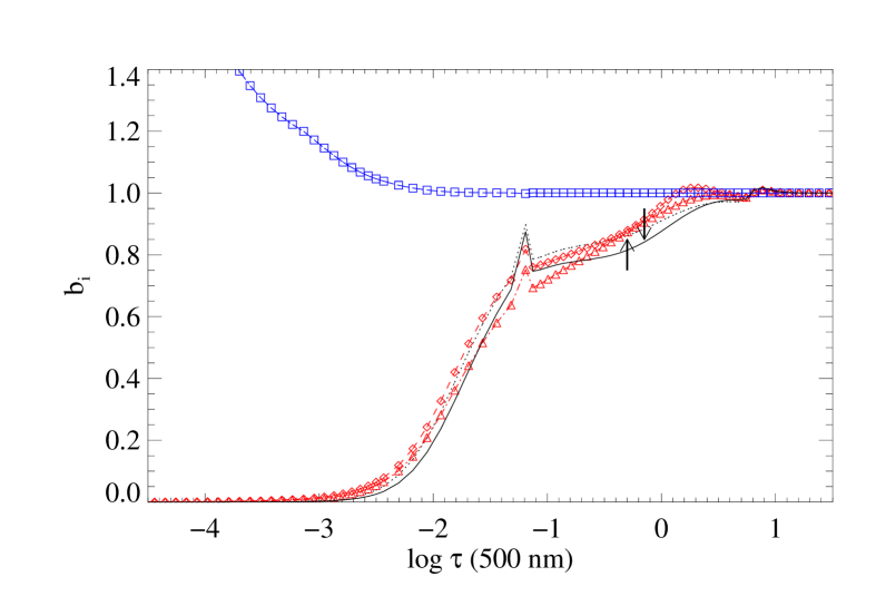
Figure 7: The NLTE departure coefficients of Ti i for RSG models with log g = -0.5, [Z] = -0.5 and T_eff = 3400K (top) and 4400K (bottom). Blue: Ti ii ground state $a\,^{4}{\rm F}$. Black: lower fine structure levels of J-band IR transitions, $b\,^{3}{\rm F}_{\rm 3}$ (dotted), $b\,^{3}{\rm F}_{\rm 2}$ (solid). Red: upper fine structure levels of IR-transitions, $z\,^{3}{\rm D}^{{\rm\circ}}_{\rm 2}$ (triangles), $z\,^{3}{\rm D}^{{\rm\circ}}_{\rm 1}$ (diamonds). The LTE and NLTE line center optical depths $\log\tau(11949.58$ Å, Ti i$)=0$ are also indicated by the upward and downward directed arrows, respectively.

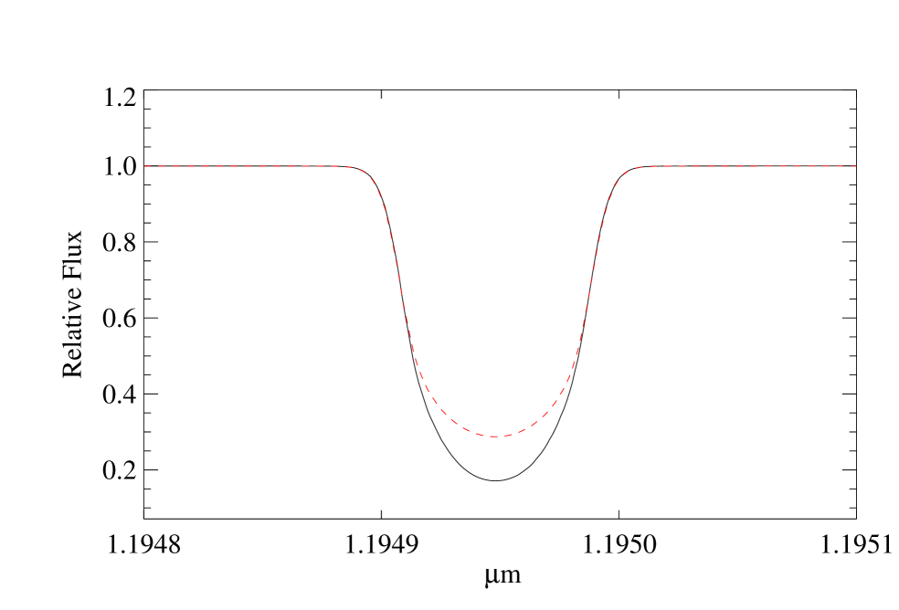
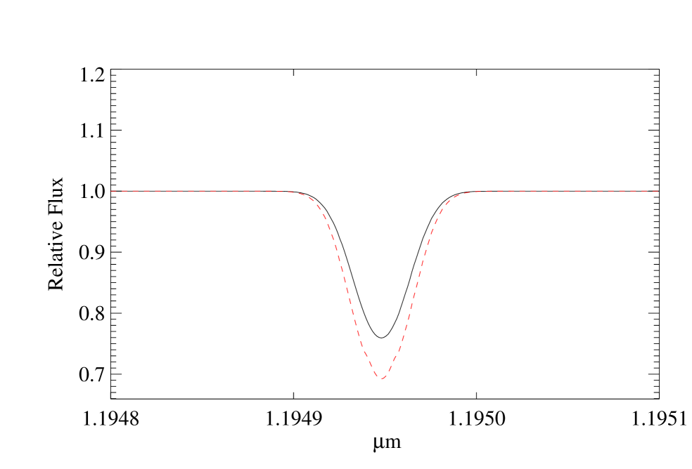
Figure 8: The NLTE (black, solid) and LTE (red, dashed) profiles of the Ti iline at $11949.58$ Å computed for log g = -0.5 and [Z] = -0.5 with microturbulence $\xi_{\rm t}=5$ km/s and T_eff = 3400K (top) and 4400K (bottom).

4.3 Equivalent widths and non-LTE abundance corrections

The NLTE and LTE abundance corrections and equivalent widths for the individual Ti i and Fe i J-band lines studied are given in Tables 2 to 5. Fig. 9 shows the NLTE abundance corrections for some of these lines computed using $\xi=2$ km s^-1 as a function of effective temperature, gravity and metallicity. The results for microturbulence 5 km s^-1 are not shown because they are nearly identical. As a consequence of the small Fe i NLTE effects discussed in section 4.1 the NLTE abundance corrections are very small and reach a maximum value $\sim$ 0.1 dex only at the highest effective temperature. The medium resolution J-band $\chi^{2}$ fitting method of RSG spectra developed by DKF10 achieves an accuracy of $0.15$ dex on average for the metallicity of an individual RSG. Thus, we do not expect NLTE effects in Fe i to heavily affect the results.

On the other hand, the NLTE effects for Ti i are more pronounced as discussed in section 3.2. This is clearly reflected in the NLTE abundance corrections, which become $\sim-0.4$ dex at low effective temperatures and change to $\sim 0.2$ dex at high effective temperature. Thus, if the Ti i lines were the only features to derive stellar metallicities from J-band spectra, NLTE effects would imply large corrections. However, the technique introduced by DKF10 uses the full information of many J-band lines from different atomic species (7 Fe i, 2 Mg i, 2 Ti i, 3 Si i lines) simultaneously to determine metallicity together with stellar parameters. Since the Fe i lines are only weakly affected by NLTE, we expect Ti i NLTE effects to have a smaller influence on the determination of the overall metallicity than the NLTE abundance corrections for the Ti i near-IR lines only.

4.4 J-band medium resolution spectral analysis

In order to assess the influence of the NLTE effects on the J-band medium resolution metallicity studies, we have carried out the following experiment. We calculated complete synthetic J-band spectra with MARCS model atmospheres and LTE opacities for all spectral lines except the Fe i and Ti i  for which we used our NLTE calculations. We then used these synthetic spectra calculated for T_eff from 3400K to 4400K with different log g and different metallicity (and with added Gaussian noise corresponding to S/N of $200$) as input for the DKF10 $\chi^{2}$ analysis using MARCS model spectra calculated completely in LTE. The metallicity grid for the MARCS model spectra had a resolution of 0.25 dex between [Z] = -1 and +0.5 and a cubic spline interpolation was used between the grid points (see Evans et al. 2011). From the metallicities recovered in this way we can estimate the possible systematic errors when relying on a complete LTE fit of RSG J-band spectra.

We found small average metallicity corrections of $-0.15$ dex at low temperatures and $+0.1$ dex at high temperatures with only a weak dependence on input metallicity (Fig. 11). This qualitative behaviour is as expected given the results shown in Fig. 9 and 10. Quantitatively, the effects are small, since the results of these tests are dominated by the Fe i lines, which are more numerous than the Ti i lines and for which the behavior NLTE corrections are minor (note that in this paper we have only discussed the non-LTE effects of the four strongest Fe i lines). The [Z] resolution of the model grid for this experiment is 0.25 dex and we know that the systematics uncertainties of the analysis technique are of the order of 0.15 dex (DKF10), thus, the NLTE corrections are marginally within the accuracy of the fitting procedure. However, very obviously the inclusion of NLTE effects in the calculation of J-band Fe i and, in particular, Ti i will improve the accuracy of future work.

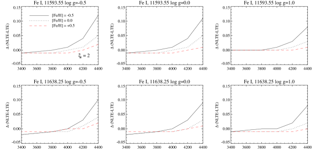
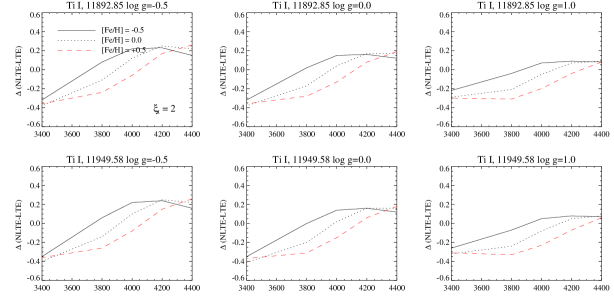
Figure 9: NLTE abundance corrections as a function of effective temperature for microturbulence $\xi$ = 2 km/s for Fe i11593 Å(top),Fe i11638 Å(2nd row), Ti i11893 Å(3rd row) and Ti i11949 (bottom). Left column: log g = -0.5, middle column: log g = 0.0, right column: log g = 1.0. Black solid: [Z] = -0.5, blue dotted: [Z] = 0.0, red dashed: [Z] = +0.5.

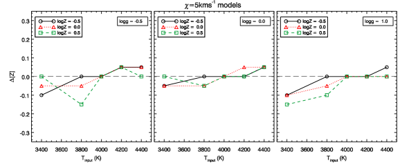
Figure 10: Influence of the TiI and FeI non-LTE effects on the DKF10 J-band $\chi^{2}$ metallicity determination as a function of effective temperature. The numerical experiment is described in the text. Left: log g $=-0.5$, middle: log g $=0.0$, right: log g $=1.0$. Circles: [Z] $=-0.5$, triangles: [Z] $=0.0$, squares: [Z] $=0.5$

4.5 Modeling uncertainties

Spectroscopic analysis of red supergiants is generally a highly non-trivial matter (Gustafsson & Plez, 1992), as other complexities arise. Among the most severe is sub-photospheric convection. At present, it is not possible to systematically evaluate the effect of 1D hydrostatic equilibrium approximation on the determination of stellar parameters from RSG spectra. The only realistic non-gray 3D radiative hydrodynamics simulation of convection for a single RSG model was performed by Chiavassa et al. (2011). They demonstrated that there is no unique 1D static model, which would provide similar observable characteristics, i.e. SED shape and colors, as the analogous 3D RHD model. To match the optical spectrum dominated by TiO opacity, a $\sim 100$ K cooler 1D model is needed, whereas the IR spectral window can be best matched using a $\sim 200$ K hotter 1D model. The NLTE effects, however, are sensitive to the radiation field across the whole spectrum, from UV to the IR. Thus, it is not possible to predict the changes in the NLTE abundance corrections simply by using a cooler or hotter 1D static model. One could, in principle, expect that, since the mean T($\tau)$ relation of a typical 3D RHD model (Chiavassa et al., 2011, their Fig. 5) is shallower than that of a corresponding 1D static model, the NLTE effects would be smaller. Our recent work on low-mass solar-like stars (Bergemann et al., 2012) showed that the largest differences in terms of NLTE effects occur at low metallicities, where 3D models are up to $1000$ K cooler than 1D hydrostatic models. The RSG models investigated in this work have metallicities close to solar. In any case, full NLTE calculations adopting, at least, a mean structure of the 3D RHD model, are necessary. Given our recent experience with calculations of such type for the solar-like stars (Bergemann et al. 2012), we are now in position to perform similar analysis for RSG’s.

5 Conclusions and Future Work

We have presented detailed calculations of the non-LTE effects in Fe i and Ti i lines in the J-band, relevant to the analysis technique of DFK10. The non-LTE corrections to abundances measured from individual Fe i lines are small – less than $0.15$ dex across the parameter range studied. On the other hand, for Ti i these corrections are larger, $0.4$ dex at the extreme. However, as there are only two Ti i lines in the J-band spectral window compared to many Fe i lines and other lines of other elements such as Mg i and Si i  the impact on the derived metallicity of a given spectrum is small. Differential analysis of non-LTE corrected and uncorrected spectra shows that the average difference in measured metallicity $[Z]$ is $\lesssim$ 0.15 dex, i.e. still within the accuracy range of the medium resolution analysis procedure but large enough and showing systematic trends with $T_{\rm eff}$ and $[Z]$ that it seems worthwhile to include the non-LTE effects in the calculation of the J-band synthetic spectra. This will ultimately improve the accuracy of the method, in particular, when it will be applied not only to measure overall metallicity but also individual element abundances and the diagnostically important ratio of $\alpha$ to iron elements.

In terms of future work, we will next turn our attention to the other prominent species in the $J$-band spectral window, namely those of Si i and Mg i. These lines also contain important metallicity information, since they help constrain the measurement of a star’s $\alpha$-element abundance. In order to determine the non-LTE corrections to the $J$-band transitions of these species we have already begun to construct model atoms, and the computation of the NLTE line strengths will begin shortly.

Table 1: J-band Fe i and Ti i lines

Elem.	$\lambda$	$E_{\rm low}$	lower	$E_{\rm up}$	upper	$log~{}gf$
	Å	[eV]	level	[eV]	level
(1)	(2)	(3)	(4)	(5)	(6)	(7)
Ti i	11892.85	1.43	$b\,^{3}{\rm F}_{\rm 2}$	2.47	$z\,^{3}{\rm D}^{{\rm\circ}}_{\rm 1}$	-1.908
	11949.58	1.44	$b\,^{3}{\rm F}_{\rm 3}$	2.48	$z\,^{3}{\rm D}^{{\rm\circ}}_{\rm 2}$	-1.760
Fe i	11638.25	2.18	$a\,^{5}{\rm P}_{\rm 3}$	3.25	$z\,^{5}{\rm D}^{{\rm\circ}}_{\rm 3}$	-2.214
	11973.01	2.18	$a\,^{5}{\rm P}_{\rm 3}$	3.22	$z\,^{5}{\rm D}^{{\rm\circ}}_{\rm 4}$	-1.483
	11882.80	2.20	$a\,^{5}{\rm P}_{\rm 2}$	3.24	$z\,^{5}{\rm D}^{{\rm\circ}}_{\rm 3}$	-1.668
	11593.55	2.22	$a\,^{5}{\rm P}_{\rm 1}$	3.29	$z\,^{5}{\rm D}^{{\rm\circ}}_{\rm 0}$	-2.448

Table 2: Non-LTE abundance corrections for the Ti i and Fe i lines ($\xi$ = 2 kms^-1)

Teff	$log~{}g$	[Z]	$\Delta_{\rm TiI}$	$\Delta_{\rm TiI}$	$\Delta_{\rm FeI}$	$\Delta_{\rm FeI}$	$\Delta_{\rm FeI}$	$\Delta_{\rm FeI}$
			$11892.85$	$11949.58$	$11593.55$	$11638.25$	$11882.80$	$11973.01$
(1)	(2)	(3)	(4)	(5)	(6)	(7)	(8)	(9)
4400.	-0.50	0.50	0.26	0.26	0.02	0.02	0.02	0.02
4400.	-0.50	0.00	0.22	0.22	0.05	0.04	0.03	0.03
4400.	-0.50	-0.50	0.15	0.16	0.12	0.10	0.08	0.07
4400.	0.00	0.50	0.19	0.18	0.01	0.01	0.01	0.01
4400.	0.00	0.00	0.17	0.16	0.05	0.03	0.02	0.02
4400.	0.00	-0.50	0.12	0.12	0.11	0.09	0.07	0.06
4400.	1.00	0.50	0.08	0.06	0.01	0.00	-0.01	-0.01
4400.	1.00	0.00	0.09	0.08	0.03	0.02	0.01	0.01
4400.	1.00	-0.50	0.08	0.07	0.08	0.08	0.05	0.05

Note. — This table is published in its entirety in the electronic edition of ApJ. A portion is shown here for guidance regarding its form and content.

Table 3: Non-LTE abundance corrections for the Ti i and Fe i lines ($\xi$ = 5 kms^-1)

Teff	$log~{}g$	[Z]	$\Delta_{\rm TiI}$	$\Delta_{\rm TiI}$	$\Delta_{\rm FeI}$	$\Delta_{\rm FeI}$	$\Delta_{\rm FeI}$	$\Delta_{\rm FeI}$
			$11892.85$	$11949.58$	$11593.55$	$11638.25$	$11882.80$	$11973.01$
(1)	(2)	(3)	(4)	(5)	(6)	(7)	(8)	(9)
4400.	-0.50	0.00	0.25	0.25	0.03	0.03	0.03	0.03
4400.	-0.50	0.00	0.22	0.22	0.06	0.06	0.04	0.04
4400.	-0.50	-0.50	0.17	0.16	0.12	0.12	0.11	0.11
4400.	0.00	0.50	0.20	0.20	0.02	0.01	0.00	0.01
4400.	0.00	0.00	0.17	0.17	0.06	0.05	0.03	0.03
4400.	0.00	-0.50	0.15	0.14	0.11	0.11	0.10	0.10
4400.	1.00	0.50	0.11	0.10	0.01	0.00	-0.02	-0.02
4400.	1.00	0.00	0.11	0.11	0.04	0.03	0.02	0.01
4400.	1.00	-0.50	0.12	0.10	0.08	0.09	0.08	0.08

Note. — This table is published in its entirety in the electronic edition of ApJ. A portion is shown here for guidance regarding its form and content.

Table 4: Equivalent widths of the Ti i and Fe i lines ($\xi$ = 2 kms^-1)

Teff	$log~{}g$	[Z]	$W_{\lambda,\rm TiI}$	$W_{\lambda,\rm TiI}$	$W_{\lambda,\rm TiI}$	$W_{\lambda,\rm TiI}$	$W_{\lambda,\rm FeI}$	$W_{\lambda,\rm FeI}$	$W_{\lambda,\rm FeI}$	$W_{\lambda,\rm FeI}$	$W_{\lambda,\rm FeI}$	$W_{\lambda,\rm FeI}$	$W_{\lambda,\rm FeI}$	$W_{\lambda,\rm FeI}$
			$11892$	$11892$	$11949$	$11949$	$11593$	$11593$	$11638$	$11638$	$11882$	$11882$	$11882$	$11973$
			$LTE$	$NLTE$	$LTE$	$NLTE$	$LTE$	$NLTE$	$LTE$	$NLTE$	$LTE$	$NLTE$	$LTE$	$NLTE$
(1)	(2)	(3)	(4)	(5)	(6)	(7)	(8)	(9)	(10)	(11)	(12)	(13)	(14)	(15)
4400.	-0.50	0.50	221.6	186.3	239.7	205.6	438.5	436.0	492.1	488.2	658.1	649.8	773.3	759.5
4400.	-0.50	0.00	155.8	123.2	176.2	143.3	386.5	380.7	425.9	420.4	530.0	522.5	597.4	586.5
4400.	-0.50	-0.50	80.1	61.4	98.6	77.8	336.4	324.9	370.2	358.9	443.0	431.8	483.4	470.6
4400.	0.00	0.50	218.6	194.5	236.1	213.6	428.4	426.6	482.0	480.2	647.6	643.7	762.2	754.5
4400.	0.00	0.00	149.4	126.2	168.7	146.1	373.7	368.4	413.3	408.8	518.2	512.6	585.8	577.6

Note. — This table is published in its entirety in the electronic edition of ApJ. A portion is shown here for guidance regarding its form and content.

Table 5: Equivalent widths of the Ti i and Fe i lines ($\xi$ = 5 kms^-1)

Teff	$log~{}g$	[Z]	$W_{\lambda,\rm TiI}$	$W_{\lambda,\rm TiI}$	$W_{\lambda,\rm TiI}$	$W_{\lambda,\rm TiI}$	$W_{\lambda,\rm FeI}$	$W_{\lambda,\rm FeI}$	$W_{\lambda,\rm FeI}$	$W_{\lambda,\rm FeI}$	$W_{\lambda,\rm FeI}$	$W_{\lambda,\rm FeI}$	$W_{\lambda,\rm FeI}$	$W_{\lambda,\rm FeI}$
			$11892$	$11892$	$11949$	$11949$	$11593$	$11593$	$11638$	$11638$	$11882$	$11882$	$11882$	$11973$
			$LTE$	$NLTE$	$LTE$	$NLTE$	$LTE$	$NLTE$	$LTE$	$NLTE$	$LTE$	$NLTE$	$LTE$	$NLTE$
(1)	(2)	(3)	(4)	(5)	(6)	(7)	(8)	(9)	(10)	(11)	(12)	(13)	(14)	(15)
4400.	-0.50	0.50	387.6	304.7	432.6	349.8	871.8	866.0	944.3	938.2	1111.8	1106.5	1208.6	1198.9
4400.	-0.50	0.00	234.0	170.0	278.6	209.9	781.9	768.3	850.8	838.4	990.4	980.0	1060.6	1047.5
4400.	-0.50	-0.50	96.0	68.2	123.1	91.3	678.3	651.4	748.6	722.2	877.9	853.4	936.3	910.1
4400.	0.00	0.50	385.6	324.5	428.4	369.3	847.7	843.4	920.2	917.0	1088.4	1087.5	1186.2	1181.5
4400.	0.00	0.00	225.4	176.5	268.0	216.7	751.8	739.6	820.4	809.8	960.5	952.4	1031.2	1020.8

Note. — This table is published in its entirety in the electronic edition of ApJ. A portion is shown here for guidance regarding its form and content.

References

- Allen (1973) Allen, C. W. 1973, London: University of London, Athlone Press, —c1973, 3rd ed.,
- Allende Prieto et al. (2001) Allende Prieto, C., Lambert, D. L., & Asplund, M. 2001, ApJ, 556, L63
- Barklem et al. (2011) Barklem, P. S., Belyaev, A. K., Guitou, M., et al. 2011, A&A, 530, A94
- Barklem et al. (2012) Barklem, P. S., Belyaev, A. K., Spielfiedel, A., Guitou, M., & Feautrier, N. 2012, arXiv:1203.4877
- Bautista (1997) Bautista, M. A. 1997, A&AS, 122, 167
- Bergemann (2011) Bergemann, M. 2011, MNRAS, 413, 2184
- Bergemann et al. (2012) Bergemann, M., Lind, K., Collet, R., Magic, Z., Asplund, M. 2012, MNRAS, submitted
- Bresolin et al. (2009) Bresolin, F., Gieren, W., Kudritzki, R.-P., et al. 2009, ApJ, 700, 309
- Brooks et al. (2007) Brooks, A. M., Governato, F., Booth, C. M., et al. 2007, ApJ, 655, L17
- Brott & Hauschildt (2005) Brott, A. M., Hauschildt, P. H., “A PHOENIX Model Atsmophere Grid for GAIA”, ESAsp, 567, 565
- Butler & Giddings (1985) Butler, K., Giddings, J. 1985, Newsletter on Analysis of Astronomical Spectra No. 9, University College London
- Chiavassa et al. (2011) Chiavassa, A., Freytag, B., Masseron, T., & Plez, B. 2011, A&A, 535, A22
- Colavitti et al. (2008) Colavitti, E., Matteucci, F., & Murante, G. 2008, A&A, 483, 401
- Davidge (2009) Davidge, T. J. 2009, ApJ, 697, 1439
- Davé et al. (2011a) Davé, R., Oppenheimer, B. D., & Finlator, K. 2011, MNRAS, 415, 11 (a)
- Davé et al. (2011b) Davé, R., Finlator, K., & Oppenheimer, B. D. 2011, MNRAS, 416, 1354 (b)
- Davies et al. (2009a) Davies, B., Origlia, L., Kudritzki, R. P., et al. 2009, ApJ, 696, 46 (a)
- Davies et al. (2009b) Davies, B., Origlia, L., Kudritzki, R. P., et al. 2009, ApJ, 696, 2014 (b)
- Davies et al. (2010) Davies, B., Kudritzki, R. P., & Figer, D. F. 2010, MNRAS, 407, 1203 (b)
- De Lucia et al. (2004) De Lucia, G., Kauffmann, G., & White, S. D. M. 2004, MNRAS, 349, 1101
- de Rossi et al. (2007) de Rossi, M. E., Tissera, P. B., & Scannapieco, C. 2007, MNRAS, 374, 323
- Evans et al. (2011) Evans, C. J., Davies, B., Kudritzki, R. P., et al. 2011, A&A, 527, 50
- Finlator & Davé (2008) Finlator, K., & Davé, R. 2008, MNRAS, 385, 2181
- Garnett & Shields (1987) Garnett, D. R., & Shields, G. A. 1987, ApJ, 317, 82
- Garnett et al. (1997) Garnett, D. R., Shields, G. A., Skillman, E. D., Sagan, S. P., & Dufour, R. J. 1997, ApJ, 489, 63
- Garnett (2004) Garnett, D. R. 2004, In: Cosmochemistry. The melting pot of the elements. Cambridge contempuary astrophysics. Cambridge, UK: Cambridge University Press, p.171 - 216.
- Gehren et al. (2001) Gehren, T., Korn, A. J., & Shi, J. 2001, A&A, 380, 645
- Gehren et al. (2001) Gehren, T., Butler, K., Mashonkina, L., Reetz, J., & Shi, J. 2001, A&A, 366, 981
- Grevesse et al. (2007) Grevesse, N., Asplund, M,& Sauval, A. J. 2007, Space Sci. Rev., 130, 105
- Gustafsson & Plez (1992) Gustafsson, B., & Plez, B. 1992, Instabilities in Evolved Super- and Hypergiants, 86
- Gustafsson et al. (2008) Gustafsson, B., Edvardsson, B., Eriksson, K., Jorgensen, U. G., Nordlund, A, & Plez, B. 2008, A&A, 486, 951
- Hauschildt et al. (1997) Hauschildt, P. H., Allard, F., Alexander, D. R., & Baron, E. 1997, ApJ, 488, 428
- Heiter & Eriksson (2006) Heiter, U. & Eriksson, B. 2006,A&A, 452, 2039
- Hou et al. (2000) Hou, J. L., Prantzos, N., & Boissier, S. 2000, A&A, 362, 921
- Kewley & Ellison (2008) Kewley, L. J., & Ellison, S. L. 2008, ApJ, 681, 1183
- Köppen et al. (2007) Köppen, J., Weidner, C., & Kroupa, P. 2007, MNRAS, 375, 673
- Kudritzki et al. (2008) Kudritzki, R.-P., Urbaneja, M. A., Bresolin, F., et al. 2008, ApJ, 681, 269
- Kudritzki (2010) Kudritzki, R. P., Astronomical Notes, 331, 459
- Kudritzki et al. (2012) Kudritzki, R.-P., Urbaneja, M. A., Gazak, Z., et al. 2012, ApJ, in press
- Kupka et al. (2000) Kupka, F. G., Ryabchikova, T. A., Piskunov, N. E., Stempels, H. C., & Weiss, W. W. 2000, Baltic Astronomy, 9, 590
- Kupka et al. (1999) Kupka, F., Piskunov, N., Ryabchikova, T. A., Stempels, H. C., & Weiss, W. W. 1999, A&AS, 138, 119
- Lequeux et al. (1979) Lequeux, J., Peimbert, M., Rayo, J. F., Serrano, A., & Torres-Peimbert, S. 1979, A&A, 80, 155
- Lee et al. (2006) Lee, H., Skillman, E.D., Cannon, J.M., et al. 2006, ApJ, 647, 970
- Lind et al. (2011) Lind, K., Asplund, M., Barklem, P. S., & Belyaev, A. K. 2011, A&A, 528, A103
- Lind et al. (2012) Lind, K., Bergemann, M., Asplund, M. 2012, MNRAS, submitted
- Maiolino et al. (2008) Maiolino, R., Nagao, T., Grazian, A., et al. 2008, A&A, 488, 463
- Mashonkina (1996) Mashonkina, L. J. 1996, M.A.S.S., Model Atmospheres and Spectrum Synthesis, 108, 140
- Mashonkina et al. (2011) Mashonkina, L., Gehren, T., Shi, J.-R., Korn, A. J., & Grupp, F. 2011, A&A, 528, A87
- Meynet & Maeder (2003) Meynet, G., & Maeder, A. 2003, A&A, 404, 975
- Naab & Ostriker (2006) Naab, T., & Ostriker, J. P. 2006, MNRAS, 366, 899
- O’Brian et al. (1991) O’Brian, T. R., Wickliffe, M. E., Lawler, J. E., Whaling, W., & Brault, J. W. 1991, Journal of the Optical Society of America B Optical Physics, 8, 1185
- Paturel et al. (2003) Paturel, G., Petit, C., Prugniel, P., et al. 2003, A&A, 412, 45
- Piskunov et al. (1995) Piskunov, N. E., Kupka, F., Ryabchikova, T. A., Weiss, W. W., & Jeffery, C. S. 1995, A&AS, 112, 525
- Plez (1998) Plez, B. 1998, A&A, 337, 495
- Plez (2010) Plez, B. 2010, ASPC 425, 124
- Prantzos & Boissier (2000) Prantzos, N., & Boissier, S. 2000, MNRAS, 313, 338
- Przybilla et al. (2006) Przybilla, N., Butler, K., Becker, S. R., & Kudritzki, R. P. 2006, A&A, 445, 1099
- Ralchenko et al. (2012) Ralchenko, Yu., Kramida, A.E., Reader, J., & NIST ASD Team (2011). NIST Atomic Spectra Database (ver. 4.1.0), [Online]. Available: http://physics.nist.gov/asd [2012, March 24]. National Institute of Standards and Technology, Gaithersburg, MD.
- Ryabchikova et al. (1997) Ryabchikova, T. A., Piskunov, N. E., Kupka, F., & Weiss, W. W. 1997, Baltic Astronomy, 6, 244
- van Regemorter (1962) van Regemorter, H. 1962, ApJ, 136, 906
- Reetz (1999) Reetz, J. 1999, PhD thesis, LMU München
- Rybicki & Hummer (1991) Rybicki, G. B., & Hummer, D. G. 1991, A&A, 245, 171
- Rybicki & Hummer (1992) Rybicki, G. B., & Hummer, D. G. 1992, A&A, 262, 209
- Sánchez-Blázquez et al. (2009) Sánchez-Blázquez, P., Courty, S., Gibson, B. K., & Brook, C. B. 2009, MNRAS, 398, 591
- Santiago-Cortés et al. (2010) Santiago-Cortés, M., Mayya, Y. D., & Rosa-González, D. 2010, MNRAS, 405, 1293
- Seaton (1962) Seaton, M. J. 1962, Atomic and Molecular Processes, 375
- Skillman (1998) Skillman, E. D. 1998, Stellar astrophysics for the local group: VIII Canary Islands Winter School of Astrophysics, 457
- Steenbock & Holweger (1984) Steenbock, W., & Holweger, H. 1984, A&A, 130, 319
- Tremonti et al. (2004) Tremonti, C. A., Heckman, T. M., Kauffmann, G., et al. 2004, ApJ, 613, 898
- Wiersma et al. (2009) Wiersma, R. P. C., Schaye, J., & Smith, B. D. 2009, MNRAS, 393, 99
- Yin et al. (2009) Yin, J., Hou, J. L., Prantzos, N., et al. 2009, A&A, 505, 497