Multi-horizon spherically symmetric spacetimes with several scales of vacuum energy

Kirill Bronnikov^a,b,1, Irina Dymnikova^c,d,2, and Evgeny Galaktionov^d

^a VNIIMS, 46 Ozyornaya St., Moscow, Russia

^b Institute of Gravitation and Cosmology, PFUR, 6 Miklukho-Maklaya St., Moscow 117198, Russia

^c Dept. of Math.& Comp. Sci., Univ.of Warmia & Mazury, Słoneczna 54, 10-710 Olsztyn, Poland

^d A.F. Ioffe Physico-Technical Institute, Polytekhnicheskaja 26, 194021 St.Petersburg, Russia

Abstract

We present a family of spherically symmetric multi-horizon spacetimes with a vacuum dark fluid, associated with a time-dependent and spatially inhomogeneous cosmological term. The vacuum dark fluid is defined in a model-independent way by the symmetry of its stress-energy tensor, i.e., its invariance under Lorentz boosts in a distinguished spatial direction ($p_{r}=-\rho$ for spherical symmetry), which makes the dark fluid essentially anisotropic and allows its density to evolve. The related cosmological models belong to the Lemaître class of models with anisotropic fluids and describe a universe with several scales of vacuum energy related to phase transitions during its evolution. The typical behavior of solutions and the number of spacetime horizons are determined by the number of vacuum scales. We study in detail a model with three vacuum scales: GUT, QCD and that responsible for the present accelerated expansion. The model parameters are fixed by the observational data and by analyticity and causality conditions. We find that our Universe has three horizons. During the first inflation the Universe enters a T-region which makes the expansion irreversible. After the second phase transition at the QCD scale the Universe enters an R-region, where for a long time its geometry remains almost pseudo-Euclidean. After crossing the third horizon related to the present vacuum density, the Universe should enter the next T-region with inevitable expansion.

PACS numbers: 04.70.Bw, 04.20.Dw, 04.20.Gz, 98.80.Hw

1. Introduction

Astronomical observations give a compelling evidence for the existence of a dark energy dominating our Universe at above 73 % of its density and responsible for its accelerated expansion due to negative pressure, $p=w\rho$, $w<-1/3$ [1–9] with the best fit $w=-1$ [10–15] which corresponds to the Einstein cosmological term $\lambda g_{\mu\nu}$ related to the de Sitter vacuum $T_{\mu\nu}=8\pi G\rho{}_{\rm(vac)}g_{\mu\nu}$ ($\lambda=8\pi G\rho{}_{\rm(vac)}$).

The well-known cosmological constant problem has two aspects: (i) Quantum field theory predicts for $\rho{}_{\rm(vac)}$ the Planck scale $\rho{}_{\rm(vac)}=\rho_{\rm Pl}=5\times{10^{93}}\ {\rm g/cm^{3}}$. Confronting this with the observational value, $\rho{}_{\rm(vac)}\simeq 3.6\times{10^{-30}}\ {\rm g/cm^{3}}=1.4\times{10^{-123}}\rho_{\rm Pl}$, creates the Fine-Tuning Problem. (ii) The inflationary paradigm needs a large value of $\rho{}_{\rm(vac)}$ at the beginning of the Universe evolution, typically of the GUT scale $\rho{}_{\rm(vac)}\simeq{\rho_{\rm GUT}}\simeq 5\times 10^{77}\ {\rm g/cm^{3}}$; the observations indicate its much smaller value while the Einstein equations require $\rho{}_{\rm(vac)}={\rm const}$.

A typical solution which can be found in the literature, is to put $\rho{}_{\rm(vac)}=0$ for some reason and to introduce a dark energy of non-vacuum origin which mimics the cosmological constant $\lambda$ when necessary. A lot of theories and models have been developed to describe a dynamical dark energy (for a comprehensive review see [9, 10]). The alternative to the cosmological constant provided by quintessence assumes the existence of a hypothetical component of matter content with $w_{Q}\neq-1$ [17]. Q-models based on a scalar field, rolling down its self-interaction potential [18], were tested using different methods with WMAP–CMB data. This gave the constraint $w_{Q}\leq-0.7$, with the best fit $w_{Q}=-1$ [19] which evidently corresponds to the cosmological constant $\lambda$.

Quartessence models describe a transition from a dust-dominated stage to a late-time inflationary stage. The Chaplygin gas model, with the postulated equation of state $p=-A/\rho$, gives a flat FRW model interpolating between $p=0$ and a negative pressure at late times [20]. It can be obtained in the model of a superfluid Chaplygin gas with the potential $V(\phi^{*}\phi)=M\left(\phi^{*}\phi/\mu+\mu/\phi^{*}\phi\right)$ which gives $p=-4M^{2}/\rho$ [21, 22]. In the holographic dark energy approach (see for a recent review [23]) with an interaction between dark matter with $p=0$ and dark energy [24], quartessence can be recovered as an isotropic perfect fluid [25], but the perfect fluid for holographic dark energy was found to be classically unstable [26]. The generalized Chaplygin gas (GCG) model, $p=-A/{\rho}^{\alpha}$ [27], was introduced to overcome difficulties with satisfying the CMB constraints [28]. The observational constraint on the parameter $\alpha$, $0<\alpha<0.2$, implies a little difference between the GCG and $\lambda={\rm const}$ [29].

Quintom cosmology describes the dark energy in the framework of the brane-world cosmology by introducing two scalar fields, one being a quintessence and the other a phantom (for a review see [30]). The multiple-lambda cosmology [31] describes the Universe as a kind of multiverse [32] filled with phantom energy; it may describe the evolution as a sequence of transitions between different inflationary stages. It is based on a perfect isotropic fluid with a time-dependent equation of state [33], introduced phenomenologically [31] and describing phantom-non-phantom transitions [34]. One more approach to creating different effective scales of vacuum energy density rests on curvature-nonlinear multidimensional gravity with at least two extra factor spaces whose scale factors behave as scalar fields in four-dimensional space-time [35].

According to observational data, dark energy is well described by the inflationary equation of state, $p=-\rho$. The stress-energy tensor has the form

$$T_{\mu}^{\nu}=\rho{}_{\rm(vac)}\delta^{\nu}_{\mu},\ \ \ \rho{}_{\rm(vac)}={\rm const}.$$ (1)

It represents a de Sitter vacuum which generates the de Sitter geometry responsible for accelerated expansion independently of specific properties of particular models of $\rho{}_{\rm(vac)}$.

The Standard Models of cosmology and particle physics suggest a series of phase transitions that have occurred in the course of the expansion and cooling history of the Universe [36]. A connection between particle physics and cosmology predicts the first inflation related to a phase transition at the GUT (Grand Unification) scale. The first inflation solves the key problems of the standard Big Bang model ([37] and references therein) and has been confirmed by CMB observations [36]. The Standard Model of particle physics predicts another phase transition at the QCD (Quantum Chromodynamics) scale of 100 to 200 MeV ([36] and references therein) which can be related to a second inflationary stage [38]: A quasi-stable QCD vacuum state can lead to a short period of inflation (7 e-foldings) consequently diluting the net baryon to photon ratio to its presently observed value. The second inflationary stage is considered in the model of thermal inflation [39], with a duration of about 10-foldings. Arguments for a second inflation at the QCD stage also exist in an effective model of a QCD phase transition which displays a high degree of supercooling at a critical temperature of the order of 100 MeV, so that the Universe increases exponentially during the quark-hadron transition [40].

The aim of this paper is to present and study a family of cosmological solutions to the Einstein equations describing a vacuum-dominated universe which several scales of vacuum energy related to phase transitions in the course of its evolution.

The gauge non-invariance of quantum cosmology leads to a connection between the gauge and the quantum spectrum of a certain physical quantity which can be specified in the framework of the minisuperspace model. There exists such a particular gauge in which the cosmological constant $\Lambda$ is quantized. Transitions between quantum levels of the operator $\Lambda$ can be related to several stages in the Universe evolution with different values of vacuum density $\rho{}_{\rm(vac)}$ [41].

At the classical level, the key point is the algebraic structure of the source term in the Einstein equations. In a model-independent approach, a vacuum is defined by the symmetry of its stress-energy tensor [42, 43, 44], as suggested by the Petrov classification for stress-energy tensors. The Einstein cosmological term corresponds to the maximally symmetric de Sitter vacuum with $\rho{}_{\rm(vac)}={\rm const}$. The Petrov classification of stress-energy tensors implies the existence of vacua whose symmetry is reduced as compared with (1), which allows the vacuum energy to become time-dependent and spatially inhomogeneous [44, 47, 48]. A relevant class of stress-energy tensors describes a vacuum dark fluid [49] specified by the inflationary equation of state $p_{\alpha}=-\rho$ in only one or two distinguished spatial directions, so that the vacuum dark fluid is intrinsically anisotropic.

In the spherically symmetric case, a cosmological vacuum is specified by $T^{t}_{t}=T^{r}_{r}$ ($p_{r}=-\rho$) [43, 44]. The radial direction is distinguished by the cosmological expansion. Regular solutions with source terms specified by $T^{t}_{t}=T^{r}_{r}$, necessarily have a de Sitter center [47]. In the case of two vacuum scales, at the center and at infinity, the source terms evolve from $\Lambda g_{\mu\nu}$ to $\lambda g_{\mu\nu}$ with $\lambda\ll\Lambda$ [44, 47]. The cosmological models belong to the Lemaître class of models with anisotropic pressures. They are asymptotically de Sitter at the early-time and late-time stages [50, 51].

In this paper we study, in a general setting, spherically symmetric spacetimes with several vacuum scales. The relevant Lemaître models involve several de Sitter (inflationary) stages in the Universe evolution. We study in detail a cosmological model with three basic vacuum scales: the GUT and QCD scales, and that responsible for the presently observed accelerated expansion, $\rho_{\lambda}=(8\pi G)^{-1}\lambda$. We introduce a phenomenological density profile describing vacuum decay at each stage by an exponential function, as is typical for a decay, and fix the decay rate by the conditions of analyticity and causality. This approach allows us to reveal certain general features of our Universe including the number of its spacetime horizons.

The paper is organized as follows: In Sec. 2 we introduce spherically symmetric vacuum spacetimes. In Sec. 3 we show how the number of vacuum cales determines the general features of a spacetime, including the number of horizons. In Sec. 4 we describe a transition from the static reference frame to geodesic reference frames representing Lemaître cosmologies. Sec. 5 presents a Lemaître cosmological model with a vacuum dark fluid, $T_{t}^{t}=T_{r}^{r}$. Sec. 6 describes a model with three vacuum scales, GUT, QCD and present-day vacuum density, with the parameters fixed by the observational data. In Sec. 7 we summarize and discuss the results.

2. Vacuum energy in general spherically symmetric spacetimes

A general model-independent approach based on the Petrov classification of stress-energy tensors (SETs) defines a vacuum by the symmetry properties of its SET [42, 43, 44]. The Einstein cosmological term corresponds to the de Sitter vacuum with the SET

$$T_{\mu}^{\nu}=\rho\delta^{\nu}_{\mu},\qquad p=-\rho.$$ (2)

The medium specified by (2) is interpreted as a vacuum due to the algebraic structure of its SET (2). It has an infinite set of comoving reference frames, so that an observer cannot in principle measure his/her velocity with respect to it [42], which is an intrinsic property of a vacuum [52]. The Einstein equations imply $\nabla_{\nu}T_{\mu}^{\nu}=0$, which leads to $\rho={\rm const}$ for the de Sitter vacuum (2). The maximum symmetry of the vacuum SET (2) can be reduced while keeping its vacuum identity [43], and this inevitably leads (due to $\nabla_{\nu}T_{\mu}^{\nu}=0$) to a dynamical vacuum energy [44]. The vacuum SET with a reduced symmetry, such that only one or two of its spatial eigenvalues coincide with the temporal eigenvalue, represents a vacuum dark fluid with the equation of state $p_{\alpha}=-\rho$ in the distinguished direction(s) [49].

The general time-dependent spherically symmetric spacetime is described by the metric

$$ds^{2}={\,\rm e}^{2\gamma}dt^{2}-{\,\rm e}^{2\alpha}dR^{2}-r^{2}d\Omega^{2},\qquad d\Omega^{2}=d\theta^{2}+\sin^{2}\theta d\phi^{2},$$ (3)

where $\alpha$, $\gamma$ and $r$ are functions of $R$ and $t$. The Einstein equations with source terms whose algebraic structure is specified by [43]

$$T^{t}_{t}=T^{r}_{r}\ \ \ \ (p_{r}=-\rho)$$ (4)

admit a class of regular solutions with a de Sitter center, $T_{\mu}^{\nu}=\Lambda\delta^{\nu}_{\mu}$ as $r=0$, where $\Lambda=8\pi G\rho_{0}$ corresponds to a certain fundamental scale of symmetry breaking $\rho_{0}=\rho{}_{\rm(vac)}$ at $r=0$ [47, 48].

In a comoving reference frame, the vacuum dark fluid specified by (4) is presented by the SET

$$T_{\mu}^{\nu}=\mathop{\rm diag}\nolimits(\rho,\ \rho,\ -p_{\bot},\ -p_{\bot}),$$ (5)

where $p_{r}$ and $p_{\bot}$ are the radial and transversal pressures, respectively.

It can be easily shown that under these general conditions we necessarily have $\rho=\rho(r)$ and hence also $p_{\bot}=p_{\bot}(r)$. To begin with, the tensor (5) is invariant under any coordinate transformations in the $(t,R)$ 2D subspace, which is just a definitive property of a vacuum. Moreover, if there is no material source of gravity other than (5), the system satisfies all conditions of the generalized Birkhoff theorem [53, 54], whence it follows that there exists a coordinate frame $(t,R)$ in which the metric (3) is $t$-independent, and consequently $\rho$ and $p_{\bot}$ are functions of $R$ alone. Let us show, however, that it is unnecessary to assume that (5) is the only source of gravity: it is sufficient to require that it does not interact with other kinds of matter, and thus the conservation law $\nabla_{\nu}T_{\mu}^{\nu}=0$ holds.

Indeed, in this case we have (dots and primes stand for $\partial/\partial t$ and $\partial/\partial R$, respectively)

$$\dot{\rho}+2\frac{\dot{r}}{r}(\rho+p_{\bot})=0,$$ (6)

$$\rho^{\prime}+2\frac{r^{\prime}}{r}(\rho+p_{\bot})=0.$$ (7)

If $r=r(R)$, hence $\dot{r}=0$, Eq. (6) immediately gives $\rho=\rho(R)$. If, on the contrary, $r$ is $t$-dependent, so that in the most general case we can suppose $\rho=\rho(R,r)$, then (6) and (7) combined lead to $\partial\rho/\partial R=0$, as was asserted, and from (6) it then also follows

$$p_{\bot}=p_{\bot}(r)=-\rho-\frac{r}{2}\frac{d\rho}{dr}.$$ (8)

From (4) it follows $G^{0}_{0}=G^{1}_{1}$ due to the Einstein equations. In the static reference frame, using the Schwarzschild coordinate $R=r$, this gives $\alpha^{\prime}+\gamma^{\prime}=0$ in (3), whence, choosing the appropriate time scaling, we get $\alpha+\gamma=0$, and the metric (3) takes the form

$$ds^{2}=A(r)dt^{2}-\frac{dr^{2}}{A(r)}-r^{2}d\Omega^{2};\ \ \ \ ~{}A(r)=e^{2\gamma(r)}$$ (9)

where the metric function $A(r)$ is given by

$$A(r)=1-\frac{2M(r)}{r},$$ (10)

and $M(r)$ is the mass function

$$M(r)=4\pi\int_{0}^{r}\rho(x)x^{2}dx.$$ (11)

We adopt the weak energy condition, i.e., a non-negative density for any observer on a time-like curve, which is natural for cosmological models describing the evolution of our Universe. This condition requires $p_{\bot}+\rho\geq 0$ which leads, by (8), to a monotonically decreasing density profile $\rho(r)$ [47]. This fact, together with the number of vacuum scales at which $p_{\bot}$ satisfies $p_{\bot}=-\rho$, determines the generic behavior of the metric function $A(r)$, and as a result the maximum number of spacetime horizons. The actual number of horizons is determined by the specific form of the profile $\rho(r)$. In Section 6 we will introduce a density profile appropriate for three vacuum scales and show how the number of horizons in our Universe follows from the observational constraints.

Eqs. (4) and (8) give an $r$-dependent equation of state. It is evident that an anisotropic fluid needs two different equation-of-state parameters $w_{\alpha}=p_{\alpha}/\rho$. In our case, $w_{r}=p_{r}/\rho=-1$ due to Eq. (4), and $w_{\bot}=p_{\bot}/\rho=-1-(r/2)d(\ln\rho)/dr$ due to Eq. (8). The parameter $w_{\bot}$ satisfies $w_{\bot}\geq-1$ since $\rho(r)$ is a monotonically decreasing function. The parameter $w_{\bot}$ approaches $w_{\bot}=-1$ as $r\to 0$, as $r\to\infty$ where $\rho$ approaches the present-day vacuum density $\rho_{\lambda}={\rm const}$, and also at each intermediate inflationary stage with $\rho{}_{\rm(vac)}={\rm const}$.

The mass function (11) can be related to the Schwarzschild mass if we separate in (11) the presently observed vacuum density $\rho_{\lambda}$ as a background density. It is possible because $\rho(r)$ is monotonically decreasing function, and $\rho_{\lambda}$ is its minimum value. If we introduce $\rho(r)=\rho_{d}+\rho_{\lambda}$, where $\rho_{d}$ is a dynamical density decreasing smoothly from the value at the center $\rho_{0}=(8\pi G)^{-1}\Lambda$ to zero at infinity, then the mass function (11) takes the form $M(r)=4\pi\int_{0}^{r}\rho_{d}(x)x^{2}dx+r^{3}\lambda/6$ and contains, in the limit $r\to\infty$, the Schwarzschild mass $M=4\pi\int_{0}^{\infty}{\rho_{d}(r)r^{2}dr}$ (in the Schwarzschild geometry it is measured by the Kepler law in the Newton limit of the Schwarzschild solution at its asymptotically flat infinity). The mass function (11) differs from the proper mass in curved spacetime, which is obtained by integration with the proper volume element $dV=\sqrt{{}^{3}g}d^{3}x$, where ${}^{3}g$ refers to the determinant of the spatial metric. The difference represents the binding energy [55], called also the gravitational mass defect [52]. The dynamics of Lemaître class models is determined by the mass function (11), therefore we do not consider here the proper mass. Let us note, however, that in the case of a cosmology which is asymptotically de Sitter at infinity, the notion of the total conserved (proper) mass of the Universe can be introduced, because any asymptotically de Sitter spacetime must have an asymptotic isometry generated by the Killing vector $\partial/\partial t$, and there exists the notion of a conserved total mass of the spacetime as computed at the future infinity [56].

3. The number of horizons and the number of scales

A typical behavior of the metric function $A(r)$ in (9) is dictated by the dynamics of the transversal pressure $p_{\bot}$ in its source (5), which determines the maximum number and nature of its extrema, determining in turn the maximum number of horizons.

According to the Einstein equations, the transversal pressure $p_{\bot}$ can be expressed in terms of the metric function $A(r)$ as

$$8\pi Gp_{\bot}={{\displaystyle\frac{1}{2}}}A^{\prime\prime}+\frac{A^{\prime}}{r}.$$ (12)

At an extremum of $A(r)$, $A^{\prime}=0$, hence, if $p_{\bot}>0$, this extremum is a minimum, and this minimum of $A$ is unique in the domain where $p_{\bot}>0$ (otherwise there would be a maximum between two minima). Assuming that $p_{\bot}$ is normally positive (so that the strong energy condition holds) and becomes negative only at distinguished spatial domains related to particular stages with a de Sitter vacuum behavior, we fix the number of zeros of $p_{\bot}$ and restrict the maximum number of zeros of $A(r)$, i.e., of spacetime horizons. One vacuum scale is related to the de Sitter center where $p_{\bot}$ is negative and $A(r)$ has a maximum. If there is no other such scale, the transversal pressure changes its sign once, and $A(r)$ has one minimum at which $A(r)$ can be negative. In the asymptotically flat case $A(r)\to 1$ as $r\to\infty$, hence one zero of $p_{\bot}$ can result in two zeros of $A(r)$, and the spacetime can have, as a maximum, two horizons [47]. If there is also a de Sitter asymptotic at infinity, this gives another domain where $p_{\bot}$ is negative. Then $A(r)$ has two maxima and can have one minimum in between where $p_{\bot}$ is positive. In this case $p_{\bot}$ changes its sign twice, and the single minimum of $A(r)$ leads to at most 3 horizons [50].

Each intermediate vacuum scale produces two more zeros of $p_{\bot}$ and at most two horizons. Hence, for $n$ vacuum scales with negative pressure we find at most $2n$ horizons in asymptotically flat spaces and at most $2n-1$ horizons in asymptotically de Sitter spaces. Note that it is the maximum number of horizons, and it will be smaller if, under the same behavior of $p_{\bot}$, the metric function is $A(r)>0$ at some of its minima or $A(r)<0$ at some of its maxima.

The dynamics of the transversal pressure also determines a typical behavior of the equation-of-state parameter $w_{\bot}$. For example, in the case of three vacuum scales of interest here, $\rho_{\rm GUT}$ at the center, $\rho_{\rm QCD}$ and $\rho_{\lambda}$, appearing successively, there can exist two domains where $p_{\bot}$ is positive. The parameter $w_{\bot}=p_{\bot}/\rho$ takes the value $w_{\bot}=-1$ during each inflationary stage, and it can be positive during the transitions $\rho_{\rm GUT}\to\rho_{\rm QCD}$, and $\rho_{\rm QCD}\to\rho_{\lambda}$.

The requirements of regularity at the center and the dominant energy condition do not restrict the total number of horizons. This can be seen from the following example.

Let $\rho>0$ and consider two extreme equations of state compatible with the dominant energy condition: (a) $p_{\bot}=-\rho$ and (b) $p_{\bot}=\rho$. In the case (a) the most general static, spherically symmetric solution is Schwarzschild-de Sitter; in the case (b) the SET structure is the same as for a radial electromagnetic field, so that we arrive at the Reissner-Nordström metric. The metric function $A$ in these two cases is

$${\rm{\bf(a)}}\qquad A(r) = 1-\frac{2m}{r}-H^{2}r^{2},$$ (13)

$${\rm{\bf(b)}}\qquad A(r) = 1-\frac{2\mu}{r}+\frac{q^{2}}{r^{2}},$$ (14)

with constant parameters $m,\ \mu,\ H,\ q$. (Note that here $q$ is not a charge, the notation is adopted for convenience).

Now, suppose that in the space-time with a regular de Sitter center the equation of state (a), leading to the exact de Sitter metric, holds in a finite interval of $r$ until $A$ reaches zero (that is, for $r<h_{1}=1/H$). Beyond this horizon let us take the equation of state (b), so that the metric function $A$ has the form (14). It matches to the solution in the previous interval of $r$ if the constants $\mu$ and $q$ are found from the continuity conditions for $A$ and $A^{\prime}$. Since $A^{\prime}(h_{1})<0$, this necessarily means that $h_{1}$ is the inner horizon of the metric (14). With growing $r$ it will eventually reach the outer horizon $r=h_{2}$ with $A^{\prime}>0$. At this point we again switch the equation of state to (a), so that the next interval will be described by $A(r)$ given in Eq. (13), with $m$ and $H$ determined from the continuity of $A$ and $A^{\prime}$. At the inevitable next horizon $h_{3}$ we will again join the Reissner-Nordström metric in the same way and so on.

The process can be continued as long as one wishes. Its feasibility is guaranteed by the following facts verified by a direct inspection:

(i) Given any $h>0$ and $C<0$, one can always find such $\mu$ and $q$ that the function (14) satisfies the conditions $A(h)=0$ and $A^{\prime}(h)=C$. Thus a next Reissner-Nordström segment can always be joined at the points $h_{1}$, $h_{3}$, etc.

(ii) Given any $h>0$ and $C>0$ such that $hC<1$, one can always find such $m$ and $H$ that the function (13) satisfies the conditions $A(h)=0$ and $A^{\prime}(h)=C$; moreover, the condition $hC<1$ always holds if $h$ is the greater of two zeros of the function (14) and $C=A^{\prime}(h)$ for the same function. Thus a next Schwarzschild-de Sitter segment can always be joined at the points $h_{2}$, $h_{4}$, etc.

The process can be stopped at any stage. If the last equation of state is (a), we obtain an asymptotically de Sitter model with an odd number of horizons; on the contrary, (b) leads to an asymptotically flat model with an even number of horizons.

The density profile is continuous but contains fractures (jumps of the derivative $\rho^{\prime}$). Where $p_{\bot}=-\rho$, we have $\rho={\rm const}$, while where $p_{\bot}=\rho$, the function $\rho(r)$ behaves as $1/r^{4}$. The fractures can, however, be smoothed by arbitrarily small additions to $\rho(r)$ without changing the whole qualitative picture, which will then correspond to an entirely smooth density distribution.

Each plateau in the density profile must, from a physical viewpoint, manifest an intermediate energy scale, eventually connected with some phase transition. We can anticipate that the existence of such scales can appreciably complicate the set of possible spacetime structures.

4. Transition to Lemaître reference frames

Consider the general static metric (9) that solves the Einstein equations with the SET (5). A transition to the geodesic coordinates $(R,\tau)$, where $\tau$ is the proper time along a geodesic and the radial coordinate $R$ is the congruence parameter, different for different geodesics, can be described in a general form. A radial timelike geodesic in the metric (9) satisfies the equations

$$\biggl{(}\frac{dr}{d\tau}\biggr{)}^{2}=E^{2}-A(r),\qquad\frac{dt}{d\tau}=\frac{E}{A(r)},$$ (15)

where the constant $E$ is connected with the initial velocity of a particle moving along this particular geodesic at a given value of the congruence parameter $R$. In general, $E=E(R)$, i.e., it is different for different geodesics.

Eqs. (15) give two of the four components of the transition matrix $\|\partial(t,r)/\partial(\tau,R)\|$, namely, $\dot{r}$ and $\dot{t}$ (dots and primes stand for $\partial/\partial\tau$ and $\partial/\partial R$, respectively) since this partial differentiation occurs along the geodesics:

$$\dot{r}=\pm\sqrt{E^{2}(R)-A(r)},\hskip 28.45274pt\dot{t}=E(R)/A(r).$$ (16)

A relation between the other two components, $t^{\prime}$ and $r^{\prime}$, can be found from the condition $g_{\tau R}=0$ when we substitute $dt=\dot{t}d\tau+t^{\prime}dR$ and $dr=\dot{r}d\tau+r^{\prime}dR$ into the metric (9):

$$t^{\prime}=\frac{\sqrt{E^{2}(R)-A(r)}}{E(R)A(r)}r^{\prime}.$$ (17)

It remains to determine $r^{\prime}(R,\tau)$, which can be done by using the integrability condition $(\partial_{\tau}\partial_{R}-\partial_{R}\partial_{\tau})r=0$. The latter takes the form of a linear first-order differential equation with respect to $r^{\prime}=y(R,r)$:

$$\partial_{r}y=-\frac{y\ \partial_{r}A}{2(E^{2}-A)}+\frac{EE^{\prime}}{E^{2}-A}.$$ (18)

Solving it, we obtain

$$y=r^{\prime}(R,\tau)=\sqrt{E^{2}-A}\Biggl{[}f_{0}(R)+EE^{\prime}\int\frac{dr}{\big{(}E^{2}-A(r)\big{)}^{3/2}}\Biggr{]}.$$ (19)

The other integrability condition $(\partial_{\tau}\partial_{R}-\partial_{R}\partial_{\tau})t=0$ holds automatically if (18) holds. The functions $t(R,\tau)$ and $r(R,\tau)$ can now be found by further integration of Eqs. (16)–(19). The resulting metric can be written as follows:

$$ds^{2}=d\tau^{2}-\frac{r^{\prime}(R,\tau)^{2}}{E^{2}(R)}dR^{2}-r^{2}(R,\tau)d\Omega^{2}.$$ (20)

One can see how this procedure works using de Sitter space as an example. Its static form is (9) with $A(r)=1-H^{2}r^{2}$, $H={\rm const}$. We will choose three different families of geodesics such that

$$E(R)=\sqrt{1-KR^{2}},\hskip 28.45274ptK=0,\pm 1,$$ (21)

and show that their corresponding reference frames represent the three well-known forms of the de Sitter metric as isotropic cosmologies with different signs of spatial curvature (see, e.g., [57]). Indeed, integrating the first relation in (16) as an equation for $\tau=\tau(r,R)$ and properly choosing the arbitrary function of $R$ that appears as an integration constant, we obtain the following expressions for $r$:

$$r(R,\tau)=(R/H)\times\Big{\{}\cosh(H\tau),\ {\,\rm e}^{H\tau},\ \sinh(H\tau)\Big{\}},$$ (22)

where the expressions in the curly brackets are ordered according to $K=1,\ 0,\ -1$. Substituting them into (20), we obtain the metric in the form

$${}ds^{2}=d\tau^{2}-a^{2}(\tau)\biggl{(}\frac{dR^{2}}{1-KR^{2}}+R^{2}d\Omega^{2}\biggr{)},$$

$${}a(\tau)=(1/H)\times\Big{\{}\cosh(H\tau),\ {\,\rm e}^{H\tau},\ \sinh(H\tau)\Big{\}},$$ (23)

as was intended. One can also verify that the expression (19) with $E(R)$ given by (21) (provided the function $f_{0}(R)$ is chosen properly) coincides with the expression for $r^{\prime}$ obtained directly from (22) in all three variants. So the transition has been completed.

5. Lemaître cosmology with vacuum dark fluid $T^{t}_{t}=T_{r}^{r}$

We have shown above that the behavior of the static metric function $A(r)$ is dictated by the number of vacuum scales, and that the static spherically symmetric metric (9) can always be transformed to the Lemaître form. Hence the cosmological evolution in this case can be described by a model from the Lemaître class satisfying the condition $p_{r}=-\rho$ that specifies a vacuum dark fluid, with the appropriate choice of the density profile $\rho(r)$ modelling smoothed jumps between different values of $\rho{}_{\rm(vac)}$, which will be discussed in the next section.

A Lemaître class model is described by the line element [52]

$$ds^{2}=d\tau^{2}-e^{2\nu(R,\tau)}dR^{2}-r^{2}(R,\tau)d\Omega^{2},$$ (24)

The coordinates $R,\tau$ are the Lagrange (comoving) coordinates. The coordinate $\tau$ measures the proper time along the world lines of a fluid. The function $r(R,\tau)$ corresponds to the Euler coordinate which is called luminosity distance.

For the metric (24), the Einstein equations with the SET (5) read [52]

$$8\pi Gp_{r} = \frac{1}{r^{2}}\left(e^{-2\nu}r^{\prime 2}-2r\ddot{r}-\dot{r}^{2}-1\right),$$ (25)

$${}8\pi Gp_{\bot} = \frac{e^{-2\nu}}{r}(r^{\prime\prime}-r^{\prime}\nu^{\prime})-\frac{\dot{r}\dot{\nu}}{r}-\ddot{\nu}-\dot{\nu}^{2}-\frac{\ddot{r}}{r},$$ (26)

$${}8\pi G\rho = -\frac{e^{-2\nu}}{r^{2}}\left(2rr^{\prime\prime}+r^{\prime 2}-2rr^{\prime}\nu^{\prime}\right)+\frac{1}{r^{2}}\left(2r\dot{r}\dot{\nu}+\dot{r}^{2}+1\right),$$ (27)

$${}8\pi GT^{r}_{t} = \frac{2e^{-2\nu}}{r}\left(\dot{r}^{\prime}-r^{\prime}\dot{\nu}\right)=0,$$ (28)

where dots and primes stand for $\partial/\partial\tau$ and $\partial/\partial R$.

The component $T_{t}^{r}$ of the SET vanishes in the comoving reference frame since there is no momentum in the radial direction, and Eq. (28) is integrated giving [52, 58]

$$e^{2\nu}=\frac{r^{\prime 2}}{1+f(R)},$$ (29)

where $f(R)$ is an arbitrary function. Putting (29) into (25), we obtain the equation of motion

$${\dot{r}}^{2}+2r{\ddot{r}}+8\pi Gp_{r}r^{2}=f(R).$$ (30)

Taking into account that $p_{r}+\rho=0$, the first integration of (30) gives

$${\dot{r}}^{2}=\frac{2GM(r)}{r}+f(R)+\frac{F(R)}{r},$$ (31)

where the mass function $M(r)$ is defined by

$$M(r)=4\pi\int_{0}^{r}\rho(x)x^{2}dx.$$ (32)

The arbitrary function $F(R)$ (an “integration constant” parametrized by $R$) should be chosen equal to zero for models regular at $r=0$ since $M(r)\to 0$ as $r\to 0$ where $\rho(r)\to\rho_{0}<\infty$.

The second integration of Eq. (30) gives

$$\tau-\tau_{0}(R)=\int\frac{dr}{\sqrt{2GM(r)/r+f(R)}}.$$ (33)

The new arbitrary function $\tau_{0}(R)$ due to this integration is called the bang-time function [59]. For example, in the case of the Tolman-Bondi model for dust ($p_{r}=p_{\perp}=0$), the evolution is described by $r(R,\tau)=[9GM(R)/2]^{1/3}[\tau-\tau_{0}(R)]^{2/3}$, where $\tau_{0}(R)$ is an arbitrary function of $R$ representing the Big Bang singularity surface at which $r(R,\tau)=0$ [60].

In the presently considered regular case, asymptotically de Sitter in the R-region near $r=0$, the evolution starts from the timelike regular surface $r(R,\tau)=r_{b}$. For $f(R)\geq 0$, the bang surface is $r(R,\tau)=0$, and the solution (33) near this surface reduces to

$$\tau-\tau_{0}(R)=\int\frac{dr}{\sqrt{r^{2}/r_{0}^{2}+f(R)}},$$ (34)

where

$$r_{0}=\sqrt{\frac{3}{8\pi G\rho_{0}}}$$ (35)

is the curvature radius at $r=0$, and $\rho_{0}$ is the density at $r=0$. In the case $f(R)<0$, the bang surface is $r(R,\tau)=r_{b}$ where $r_{b}$ satisfies $2GM(r)/r+f(R)=0$. For small values of $f(R)$ we can apply (34) which gives $r=r_{0}\sqrt{-f(R)}\cosh{[(\tau-\tau_{0}(R))/r_{0}]}$. For $f(R)>0$ we get $r=r_{0}\sqrt{f(R)}\sinh[(\tau-\tau_{0}(R))/r_{0}]$, and $r=r_{0}\exp[(\tau-\tau_{0}(R))/r_{0}]$ for $f(R)=0$.

Different points of the regular timelike bang surfaces start at different moments of the synchronous time $\tau$, so that the bangs are non-singular and non-simultaneous.

For $f(R)=0$ (parabolic motion), Eq. (34) gives at small $r$ the expansion law

$$r=r_{0}e^{(\tau-\tau_{0}(R))/r_{0}}$$ (36)

and

$$e^{2\nu}=\frac{r^{2}}{r_{0}^{2}}\left[\frac{d\tau_{0}(R)}{dR}\right]^{2},$$ (37)

The metric takes the FRW form with the de Sitter scale factor

$$ds^{2}=d\tau^{2}-r^{2}_{0}e^{2c\tau/r_{0}}\left(dq^{2}+q^{2}d\Omega^{2}\right),$$ (38)

where the variable $q=e^{\tau_{0}(R)/r_{0}}$ is introduced to transform the metric to the FRW form. In accordance with (36), it describes a non-singular non-simultaneous de Sitter bang from the surface $r(\tau-\tau_{0}(R)\to-\infty)=0$ [61].

The inflationary stage is followed by an anisotropic Kasner-like stage: One scale factor, corresponding to the transversal direction, is given by $r(R,\tau)$, and the other, corresponding to the radial direction, is proportional to $r^{\prime}$ according to (29), its particular form depending on the density profile $\rho(r)$ and the choice of arbitrary functions of $R$. If we choose $f(R)=0$ and $\tau(R)=R$, the metric can be approximated by [61, 50]

$$ds^{2}=d\tau^{2}-(\tau+R)^{-2/3}K(R)dR^{2}-L(\tau+R)^{4/3}d\Omega^{2},$$ (39)

where $K(R)$ is a smooth regular function and $L$ is a constant.

A similar behavior can be found for a density profile which approximates phase transitions with several scales of vacuum energy (see below). At each transition, an inflationary stage is followed by an anisotropic Kasner-like stage.

The generic behavior of the considered Lemaître class solutions is related to the function $A(r)$ expressed by (10) in terms of the mass function (32). Given the density profile $\rho(r)$, its specific form entirely determines the detailed properties of $A(r)$ and, in particular, the number of horizons.

6. Lemaître cosmology with GUT and QCD phase transitions

6.1. Basic features

According to the conventional scenario, the first inflationary stage corresponding to the GUT phase transition occurred at the GUT scale $E_{\rm GUT}\sim 10^{15}$ GeV, the relevant density being $\rho_{\rm GUT}\simeq 2.3\times 10^{77}\ {\rm g/cm^{3}}$. It was followed by a decay of vacuum energy resulting ultimately in a radiation-dominated stage. The next phase transition which could drive the second inflation [38–40] which occurred at the QCD scale $E_{\rm QCD}\sim(100\div 200)$ MeV, at about $10^{-5}$ seconds after the Big Bang, when the Hubble radius, $d_{H}=c/H$, was about 10 km [36]. The density $\rho_{\rm QCD}$ is smaller by a factor of $(E_{\rm QCD}/E_{\rm GUT})^{4}$ than the GUT density $\rho_{GUT}=\rho_{0}$, i.e., of the order of the nuclear matter density. The last inflationary stage corresponds to the presently observed dark energy density $\rho_{\lambda}$ which is about 107 orders of magnitude smaller than the GUT density.

This situation can be modelled by the density profile

$$\rho=\rho_{0}\biggl{[}1-(1-B_{1})\exp(-r_{1}^{n}/r^{n})-(B_{1}-B_{3})\exp(-r_{3}^{n}/r^{n})\biggr{]},$$ (40)

where $n,\ B_{1},\ B_{3},\ r_{1},\ r_{3}$ are constants, for which we adopt:

$$B_{1}=\rho_{\rm QCD}/\rho_{0}\approx 10^{-64},\qquad B_{3}=\rho_{\lambda}/\rho_{0}\approx 10^{-107};\qquad r_{0}<r_{1}\ll r_{3}.$$ (41)

The exponential function in (40) is chosen as a typical one for decay processes. The parameter $n$ characterizing the decay rate will be fixed below by the conditions of analyticity and causality.

We choose $f(R)\equiv 0$ in Eqs. (29)–(33) because in this case each 3-hypersurface $\tau={\rm const}$ is flat, with zero curvature [62], which guarantees fulfilment of the spatial flatness condition $\Omega=1$ required by the observational data.

Under the above choice, the model undergoes the following stages:

(a)

$r\ll r_{1}$: the first inflation, $\rho\approx\rho_{0}$; the mass function (32) is approximated by $M(r)=\frac{4\pi}{3}r^{3}$, and Eq. (33) yields, in agreement with (36),

$$\tau-\tau_{0}(R)\simeq r_{0}\ln{\frac{r}{r_{0}}}.$$ (42)

(b)

$r\sim r_{1}$: end of the first inflation since the second term in (40) becomes significant.

(c)

$r_{1}\ll r\ll r_{3}$, so that

$$\rho\approx\rho_{0}(B_{1}+r_{1}^{n}/r^{n}).$$ (43)

This stage in turn splits into two periods. As long as $r$ is sufficiently small,

$$r<r_{2},\hskip 28.45274ptr_{2}=r_{1}B_{1}^{-1/n}=10^{64/n}r_{1},$$ (44)

the second term in (43) is dominant, so that $\rho(r)$ rapidly decreases. It is an intermediate period between the first and second inflation. At $r=r_{2}$ the two terms coincide, and at $r>r_{2}$ we have $\rho\approx B_{1}\rho_{0}=\rho_{\rm QCD}={\rm const}$, which corresponds to the second inflation.

(d)

$r\sim r_{3}$: end of the second inflation since the third term in (40) becomes significant.

(e)

$r\gg r_{3}$: the density is

$$\rho\approx\rho_{0}(B_{3}+B_{1}r_{3}^{n}/r^{n}).$$ (45)

Similarly to stage (c), at some value of $r$, namely, at $r=r_{4}$ defined by

$$r_{4}=r_{3}(B_{1}/B_{3})^{1/n}=10^{43/n}r_{3}=10^{107/n}r_{1}$$ (46)

the two terms in (45) are equal. At $r_{3}<r<r_{4}$, we have one more intermediate period where $\rho(r)$ rapidly decreases, while at $r>r_{4}$ it approaches a constant corresponding to the present-day dark energy density.

The time elapsed between the first and the second inflation, $\tau_{2}-\tau_{1}$ (we denote $\tau_{i}=\tau(r_{i})$) is estimated by integrating between $r_{1}$ and $r_{2}$ in Eq. (33). To this end, we find the mass function in the same interval:

$$M(r)=4\pi\biggl{(}\int_{0}^{r_{1}}+\int_{r_{1}}^{r}\biggr{)}\rho(r)r^{2}dr.$$

In the first term we take $\rho\approx\rho_{0}$ while in the second one, in accord with (43), we approximate $\rho(r)$ by $\rho_{0}(r_{1}/r)^{n}$. Hence,

$$M(r)=\frac{4}{3}\pi\rho_{0}r_{1}^{3}+\frac{4\pi\rho_{0}r_{1}^{n}}{n-3}\biggl{(}\frac{1}{r_{1}^{n-3}}-\frac{1}{r^{n-3}}\biggr{)}.$$ (47)

In the last term, almost in the whole interval of interest, $r\gg r_{1}$, therefore for our estimation purpose we can neglect the last term thus obtaining a constant value of $M$,

$$M(r)\approx M_{2}=\frac{4\pi n}{3(n-3)}\rho_{0}r_{1}^{3}={\rm const}.$$ (48)

Substituting it into (33), we obtain

$$\tau_{2}-\tau_{1}\approx\sqrt{\frac{4(n-3)}{9n}}{r_{0}}\biggl{(}\frac{r_{2}}{r_{1}}\biggr{)}^{3/2}$$ (49)

The first restriction on the parameter $n$ is evident: $n>3$. The second constraint follows directly from the dominant energy condition which requires $p_{\bot}\leq\rho$ and guarantees that the speed of sound never exceeds the speed of light, thus maintaining causality in the course of evolution. A simple analysis of Eq. (8) for several vacuum scales shows that the difference $\rho-p_{\bot}$ as a function of $r$ decreases at each transition starting from $2\rho$ with $\rho={\rm const}$. Let us introduce the function $f_{\rm DEC}=\rho-p_{\bot}$ characterizing the dominant energy condition. According to (8), $f_{\rm DEC}=2\rho+r\rho^{\prime}/2$. It should be a decreasing function since $\rho(r)$ is monotonically decreasing, and its derivative $\rho^{\prime}$ is negative. During the first transition, this function should decrease from $2\rho_{0}=2\rho_{GUT}$ to $2\rho_{QCD}$. For the density profile (40) we have

$$f(r)=f_{\rm DEC}{\rho_{0}}^{-1}=2\left[1-(1-B_{1})e^{-r_{1}^{n}/r^{n}}\left(1+\frac{n}{4}\left(\frac{r_{1}}{r}\right)^{n}\right)\right]$$ (50)

It should be non-negative and decreasing from $2$ to $2B_{1}$, where $B_{1}=\rho_{QCD}/\rho_{GUT}$ is given by (41). For $r\gg r_{1}$ the exponent in (50) can be presented as a series in $(r_{1}/r)^{n}$ which gives

$$f=2B_{1}+2(1-B_{1})\left[\left(1-\frac{n}{4}\right)\left(\frac{r_{1}}{r}\right)^{n}+\left(\frac{n}{4}-\frac{1}{2}\right)\left(\frac{r_{1}}{r}\right)^{2n}+{\cal O}\left(\frac{r_{1}}{r}\right)^{3n}\right]$$ (51)

The condition of non-negativity of this function is $n\leq 4$. The derivative is given by

$$f^{\prime}=\frac{(1-B_{1})}{2}\frac{n}{r}\left(\frac{r_{1}}{r}\right)^{n}e^{-r_{1}^{n}/r^{n}}\left[n-4-n\left(\frac{r_{1}}{r}\right)^{n}\right]$$ (52)

The condition $n\leq 4$ guarantees a monotonic decrease of the function $\rho-p_{\bot}$ during the first transition. It is easy to show that this concerns also the second transition at which the function $f_{\rm DEC}(r)$ decreases from $2\rho_{\rm QCD}$ to $2\rho_{\lambda}$.

The condition $n\leq 4$ thus provides non-negativity of the function $f_{\rm DEC}=\rho-p_{\bot}$ during the cosmological evolution with the density profile (40). Therefore we fix $n=4$ as the only integer compatible with analyticity and causality.

Let us note that at the end of both transitions, for $r\gg r_{1}$ and $r\gg r_{3}$, the density in (40) behaves like $\rho\propto r^{-4}$, in a way typical of radiation in FRW cosmology where $\rho a^{4}={\rm const}$ and also agrees with our qualitative analysis in the second part of Section 3.

With $n=4$ we get from (47)

$$M(r)=\frac{4}{3}\pi\rho_{0}r_{1}^{3}+4\pi\rho_{0}r_{1}^{4}\biggl{(}\frac{1}{r_{1}}-\frac{1}{r}\biggr{)}.$$ (53)

The value of $M_{2}$ in (48) is now

$$M_{2}=\frac{16}{3}\pi\rho_{0}r_{1}^{3}.$$ (54)

Substituting it into (49), we obtain

$$\tau_{2}-\tau_{1}\approx\frac{r_{0}}{3}\biggl{(}\frac{r_{2}}{r_{1}}\biggr{)}^{3/2}\sim 10^{24}r_{0}.$$ (55)

Recalling that $r_{0}\sim 10^{8}\,l_{\rm pl}$, we find $\tau_{2}-\tau_{1}\sim 10^{32}\,l_{\rm pl}/c\sim 10^{-11}$ s. It is of interest that this estimate does not depend on the particular choice of the free parameter $r_{1}$ or, equivalently, the number of e-foldings $N_{e}:=\ln(r_{1}/r_{0})$.

Furthermore, if the second inflation contains 7 e-foldings [38], it means that $r_{3}\sim 10^{3}r_{2}$. It is then also easy to find $r_{4}$, the value of $r$ at which the DE density has reached its modern value, from (46): $r_{4}\sim 10^{43/4}r_{3}$. To estimate the duration of the second inflation $\tau_{3}-\tau_{2}$ and the time $\tau_{4}$ of the onset of the latest $\lambda$-dominated stage, we should integrate in (33) from $r_{2}$ to $r_{3}$ and then to $r_{4}$. Acting in the same manner as in finding $\tau_{2}$, we see that the main contribution to the mass function comes from the range $r<r_{2}$ and is given by (54), hence the duration of the second inflation is

$$\tau_{3}-\tau_{2}\approx\sqrt{\frac{1}{12\pi G\rho_{0}}}\biggl{(}\frac{r_{3}}{r_{1}}\biggr{)}^{3/2}\approx 10^{-7}\ {\rm s}.$$ (56)

Lastly, for $\tau_{4}$ we obtain the same relation as (56) but with $r_{3}$ replaced by $r_{4}$. It results in

$$\tau_{4}-\tau_{3}\sim 10^{10}\ {\rm s}\sim 1000\ {\rm years}.$$ (57)

Let us note that all these times are practically independent of the number of e-foldings $N_{e}$ during the first inflation. However, the duration of the later period up to the present epoch does depend on $N_{e}$. Namely, since at $r\gg r_{4}$ we have $\rho\approx B_{3}\rho_{0}={\rm const}$, integration in (32) at large enough $r$ gives

$$M(r)\approx(4\pi/3)B_{3}\rho_{0}r^{3},$$ (58)

and integration in (33) yields immediately

$$\tau-\tau_{0}(R)\approx 10^{18}\ {\rm s}\cdot\ln(r/r_{*}),$$ (59)

where $r_{*}\approx 10^{9}r_{4}\approx 10^{36}r_{1}$ is the value of $r$ at which the contribution of $r^{3}$ to the mass function begins to exceed $M_{2}$.

The qualitative behavior of the vacuum density profile (40) is shown schematically in Fig. 1.

Figure 1: Typical behavior of the vacuum density during the Universe evolution. Here $r_{1}$ is the end of the first inflation, $r_{2}$ and $r_{3}$ are the beginning and end of the second inflation, respectively, $r_{4}$ corresponds to achieving the present day vacuum density $\rho_{\lambda}$.

Eq. (59) gives the expansion law $r=r_{*}e^{(\tau-\tau_{0}(R))/r_{*}}$, and Eq. (29) gives for the second scale factor in (24) $e^{2\nu}=(r^{2}/r_{*}^{2})(d\tau_{0}(R)/dR)^{2}$. Introducing the variable $q=e^{\tau_{0}(R)/r_{*}}$, we transform the metric (24) to the FRW form

$$ds^{2}=d\tau^{2}-r^{2}_{*}e^{2c\tau/r_{*}}\left(dq^{2}+q^{2}d\Omega^{2}\right),$$ (60)

at the stage where the vacuum density achieves its present value.

As we have seen, the only free parameter of the model is the number of e-foldings at first inflation $N_{e}=\ln(r_{1}/r_{0})$, where the characteristic de Sitter radius for the GUT scale vacuum is $r_{0}\simeq 2.4\times 10^{-25}$ cm. The time interval corresponding to $r_{1}$ is, according to (42), approximately $10^{-35}N_{e}$ s. In the next subsection we evaluate an admissible interval for the parameter $N_{e}$ from the requirement of late-time homogeneity and isotropy.

For the density profile (40) the transversal pressure is given by

$$p_{\bot}=\rho_{0}\left[-1+(1-B_{1})\biggl{(}1+\frac{2r_{1}^{4}}{r^{4}}\biggr{)}e^{-r_{1}^{4}/r^{4}}+(B_{1}-B_{3})\biggl{(}1+\frac{2r_{3}^{4}}{r^{4}}\biggr{)}e^{-r_{3}^{4}/r^{4}}\right].$$ (61)

It satisfies the equation $p_{\bot}=-\rho$ during each inflationary stage. It has two maxima, $p_{\bot}\simeq 0.213\rho_{0}$ at $r_{m1}\simeq 1.2r_{1}$ and $p_{\bot}\simeq 0.213B_{1}\rho_{0}=0.213\rho_{\rm QCD}$ at $r_{m2}\simeq 1.2r_{2}$ and ultimately quickly achieves $p_{\bot}=-B_{3}\rho_{0}=-\rho_{\lambda}$. The behavior of the transversal pressure (61) is shown schematically in Fig. 2.

Figure 2: Typical behavior of the transversal pressure during the Universe evolution. The quantities $r_{1}$–$r_{4}$ are the same as in Fig. 1.

The parameter $w_{\bot}=-1$ during the first inflation, then it rapidly increases to $w_{\bot}\simeq 0.213$ at $r_{m1}\simeq 1.2r_{1}$, decreases to $w_{\bot}=-1$, quickly increases to $w_{\bot}\simeq 0.213$ at $r_{m2}\simeq 1.2r_{3}$, and finally approaches $w_{\bot}=-1$ as $\rho$ approaches $\rho_{\lambda}$.

6.2. Late-time homogeneity and isotropy

At $r>r_{4}$ the model evolution is governed by the small effective cosmological constant $\lambda=B_{3}\rho_{0}/(8\pi G)$ and tends to a de Sitter regime, i.e., becomes homogeneous and isotropic.

The degree of inhomogeneity can be characterized by the dimensionless parameter $(r/\rho)d\rho/dr$ showing how the density $\rho$ changes at a distance $\sim r$. By (45) with $n=4$, at $r\gg r_{4}$ this parameter is approximately equal to $4r_{4}^{4}/r^{4}$ and rapidly decreases with growing $r$.

Thus at $r\gg r_{4}$ one can estimate the degree of anisotropy of our model as is conventionally done for homogeneous models, e.g., using the anisotropy parameter [63, 64]

$${\cal A}=\frac{1}{3H^{2}}\sum_{i=1}^{3}H_{i}^{2}-1,$$ (62)

where $H_{i}={\dot{a}}_{i}/a_{i}$ are the directional Hubble parameters corresponding to the three scale factors $a_{i}(\tau)$, the dot stands for $d/d\tau$, and $H=(H_{1}+H_{2}+H_{3})/3$ is the mean Hubble parameter (see [64] for a discussion of different anisotropy characteristics). In our model with the metric (24), where $e^{2\nu}=r^{\prime}{}^{2}$ and $f(R)=0$, these scale factors are $a_{1}=|r^{\prime}|$ and $a_{2}=a_{3}=r$. The expression for $r^{\prime}$ is found from (33):

$$r^{\prime}=-\sqrt{2GM(r)/r}\tau_{0}^{\prime}(R).$$ (63)

Using this, one obtains for the anisotropy parameter

$${\cal A}=2\frac{(\dot{M}/M-3\dot{r}/r)^{2}}{(\dot{M}/M+3\dot{r}/r)^{2}}=2\biggl{[}\frac{3M_{4}-4\pi\rho_{4}r_{4}^{3}}{3M_{4}+4\pi\rho_{4}(2r^{3}-r_{4}^{3})}\biggr{]}^{2},$$ (64)

where $M_{4}=M(r_{4})$ and $\rho_{4}=\rho(r_{4})=2B_{3}\rho_{0}$ according to (45). At large $r$ the parameter ${\cal A}\sim r^{-6}$, but, as can be directly verified, this rapid decrease does not begin from $r_{4}$ but only from much larger values of $r$ because at $r\sim r_{4}$ both the numerator and the denominator of (64) are dominated by the constant $M_{4}$.

To agree with CMB observations, the vacuum contribution must be already highly isotropic (${\cal A}<10^{-6}$) when $r$ reaches the value of the scale factor $r=r_{5}\sim 10^{25}$ cm corresponding to the recombination epoch with redshifts $z\sim 1000$. This requirement constrains the possible value of the free parameter $N_{e}=\ln(r_{1}/r_{0})$. Indeed, the condition ${\cal A}(r=r_{5})<10^{-6}$ gives

$$3M_{4}<2\sqrt{2}\pi G\rho_{4}r_{5}^{3}\cdot 10^{-3}$$ (65)

(taking into account that $M_{4}\gg\pi\rho_{4}r_{4}^{3}$). In turn, $GM_{4}$ is expressed in terms of $r_{1}$. From (54) we know the value of $M_{2}=M(r_{2})=(16/3)\pi\rho_{0}r_{1}^{3}$. To find $M_{4}$, we must integrate in (32) from $r_{2}$ to $r_{4}$; it turns out, however, that this integration contributes only a relative correction of the order $10^{-7}$ to $M_{2}$. Thus

$$M_{4}\approx\frac{16}{3}\pi\rho_{0}r_{1}^{3}.$$ (66)

Comparing (66) with (65), we obtain the constraint

$$r_{1}<B_{3}^{1/3}\,r_{5}/10\approx\mbox{$\times 10^{-37}$}r_{5}=3\mbox{$\times 10^{-12}$}\ {\rm cm},\qquad N_{e}=\ln(r_{1}/r_{0})<30.$$ (67)

Hence, after the recombination time corresponding to $r=r_{5}$, the Lemaître model (24) practically behaves as a homogeneous and isotropic FRW model (60).

6.3. Evolution of the scale factors

Now, having established the constraint (67), we can discuss the model evolution at all stages.

For the spatially flat model, $f(R)=0$, the line element (24) takes the form

$$ds^{2}=d\tau^{2}-b^{2}(\tau,R)dR^{2}-r^{2}(\tau,R)d\Omega^{2},$$ (68)

where we have introduced explicitly two scale factors: $r(\tau,R)$ in accordance with (24) and $b(\tau,R)\equiv r^{\prime}(\tau,R)$ in accordance with (29). For the integration “constant” in (34) we choose $\tau_{0}(R)=-R$ to make the de Sitter asymptotics familiar. It is easily seen that in this case $\dot{r}(\tau+R)=dr/d(\tau+R)\partial(\tau+R)/\partial\tau=dr/d(\tau+R)$.

Numerical integration of the Lemaître equations during the first transition $\rho_{\rm GUT}\to\rho_{\rm QCD}$ shows an exponential growth of both scale factors at the beginning when $p_{\perp}\simeq p_{r}=-\rho$, followed by an anisotropic Kasner-like stage where the anisotropy of the pressures leads to an anisotropic expansion. The behaviors of the two scale factors $r(\tau+R),b(\tau+R)$ during the first phase transition are shown in Figs 3 and 4.

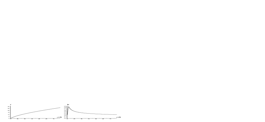
Figure 3: The behavior of the scale factors during the first phase transition. The distances are normalized to $10^{12}r_{0}$ where $r_{0}\simeq{2.4\times 10^{-25}}$ cm is the characteristic GUT length scale for $M_{\rm GUT}\simeq 10^{15}$ GeV, and the time $\tau+R$ is normalized to the GUT time $t_{\rm GUT}=r_{0}/c\simeq 0.8\times 10^{-35}$ s.

Figure 4: The behavior of the velocities $\dot{r}(\tau+R)$, $\dot{b}(\tau+R)$ at the first transition.

The behavior of the scale factors at the second phase transition is qualitatively quite the same for the density profile (40).

The evolution of the scale factors during the whole Universe history is shown schematically in Fig. 5 plotted on the basis of Fig. 3 extended to the third inflationary stage (the hypersurface $\tau+R=t_{4}$ in Fig. 5). The first inflation ends at the hypersurface $\tau+R=t_{1}$, the second inflation occurs between $\tau+R=t_{2}$ and $\tau+R=t_{3}$. The sharp maximum in ${\dot{b}}(\tau+R)$ in Fig. 4, as well as the two maxima in the right panel of Fig. 5 are related to a maximum of $p_{\bot}$ seen in Fig. 2. At late times, due to isotropy, the evolution of the two scale factors is common and conforms to the standard flat de Sitter cosmology.

Figure 5: Typical behavior of the scale factors $r(\tau+R)$ and $b(\tau+R)$.

6.4. Horizons

We have described the Universe evolution from the viewpoint of the Lemaître cosmological reference frame. Now we can find the number of horizons and present the global structure of spacetime. The proof in Sec. 3 concerned only the maximum number of horizons, and their smaller number is certainly possible, depending on the dispositions and durations of the phase transitions on the $r$ scale.

Let us find how the whole scenario looks from the static reference frame. The metric function $A(r)$ calculated with the above fixed parameters is shown in Fig. 6, where the characteristic scales designated on the $r$ axis are:

$r_{1}=10^{-12}$ cm, $N_{e}=29$ at the end of the first inflation.

$r_{2}=1.2\times 10^{4}$ cm at the beginning of the second inflation,

$r_{3}=1.2\times 10^{7}$ cm at the end of the second inflation,

$r_{4}=6.7\times 10^{17}$ cm at achieving the present-day vacuum (dark energy) density $\rho_{\lambda}$.

The values of $r_{5}=10^{25}$ cm and $r_{6}=10^{28}$ cm approximately correspond to the recombination and to the beginning of the third (presently observed) inflation, respectively. The value $r_{7}=7.5\times 10^{29}$ cm corresponds to the cosmological horizon due to de Sitter vacuum with the density $\rho_{\lambda}$. The behavior of the metric function $A(r)$, Fig. 6, testifies for the existence of three horizons for the case of the above fixed parameters corresponding to those of our Universe.

Figure 6: The metric function $A(r)$ plotted with the parameters corresponding to our Universe

The first horizon in our Universe, $r_{-}$, is close to the de Sitter radius $r_{0}$ corresponding to the GUT scale of the first phase transition. The second horizon $r_{+}\simeq 7.4\times 10^{13}$ cm distinguishes the additional essential length scale: for a long time our Universe evolves as the $T_{+}$-region $r_{-}<r<r_{+}$, i.e., the expansion is inevitable for all observers as dictated by the causal structure of spacetime. The present epoch gets into the the $R$-region between two $T_{+}$-regions. Near the point of achieving the present vacuum density the geometry generated by the vacuum fluid background becomes almost pseudo-Euclidean ($A(r)\simeq 1-10^{-6}$).

The global structure of spherically symmetric spacetime with three horizons, asymptotically de Sitter in the center and at infinity, is shown in Fig. 7 [50, 65].

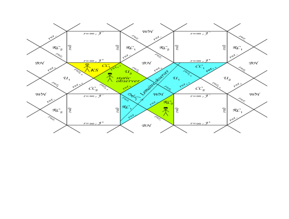
Figure 7: Global structure of spherical space-time with three horizons

This picture shows how the manifold of events is seen by different observers. Let us note that the Carter-Penrose diagram in Fig. 7 covers the whole plane except for the squares bounded by the lines $r=0$ and $r=\infty$. The lines $r_{-}$ correspond to cosmological horizons for static observers (observers in hats) in the R-regions $0\leq r<r_{-}$ denoted as ${\cal RC}$; $r_{+}$ are the black (white) hole horizons for static observers in the R-regions $r_{+}<r<r_{++}$ denoted as ${\cal U}$, and $r_{++}$ are their cosmological horizons. T₊-regions $r_{++}<r<\infty$ denoted as ${\cal CC}$ correspond to regular homogeneous anisotropic cosmological T-models of Kantowski-Sachs type [50, 51]. The Lemaître cosmological model shown in Fig. 7 starts its evolution in the R-region ${\cal RC}_{1}$ and goes consequently through the T₊-region $r_{-}<r<r_{+}$, the R-region $r_{+}<r<r_{++}$ and the T₊-region $r_{++}<r<\infty$.

7. Summary and discussion

We have presented a general analysis for the case of several scales of vacuum energy $\rho{}_{\rm(vac)}$ corresponding to phase transitions involving inflationary stages. In our approach, the vacuum dark energy is described by a vacuum dark fluid defined by symmetry of its stress-energy tensor. In the spherically symmetric case, it is invariant under radial Lorentz boosts, acquiring the maximum symmetry of de Sitter vacuum only at inflationary stages. This makes the vacuum density $\rho{}_{\rm(vac)}$ time-dependent and spatially inhomogeneous. Cosmological solutions generated by the vacuum dark fluid belong to the Lemaître class models with anisotropic pressures (their anisotropy follows directly from the variability of $\rho{}_{\rm(vac)}$).

The intrinsic properties of de Sitter space-time are responsible for an accelerated expansion, independently of particular properties of particular models of vacuum density associated with the cosmological constant. In a similar way, the intrinsic properties of geometries generated by a vacuum dark fluid can be in principle responsible for a variable vacuum density and make it possible to describe, on a common ground, the first inflationary expansion, the presently observed accelerated expansion, as well as inflationary stages related to phase transitions in the universe evolution, predicted by the Standard Model.

To our knowledge, such an approach is applied for the first time for an analysis of the cosmological evolution in the case of several vacuum scales.

The dynamics of cosmological models with a vacuum dark fluid is dictated by the number of vacuum scales: their number determines the behavior of the transversal pressure $p_{\bot}$, which in turn determines the maximum number of horizons; their actual number depends on the model parameters.

We have studied in detail the cosmological model for the case of three vacuum scales: GUT, QCD and that responsible for the presently observed accelerated expansion. We used a phenomenological density profile with a typical behavior for a cosmological scenario with inflationary stages followed by a decay of vacuum energy, which we describe by an exponential function typical of decay processes. The parameter characterizing the decay rate is tightly fixed by the requirements of analyticity and causality. Other parameters of the model are fixed by the values $\rho_{\rm GUT}$, $\rho_{\rm QCD}$, $\rho_{\lambda}$ and $\Omega=1$. The only free parameter is the number of e-foldings in the first inflation, which is estimated using the observational constraint on the CMB anisotropy.

This model reveals the following features of our Universe:

(i) Our spacetime has three horizons.

(ii) The cosmological evolution starts with a non-simultaneous timelike de Sitter bang followed by a short stage of inhomogeneous and anisotropic expansion.

(iii) During the first inflationary stage, the Universe quickly enters a T₊-region which makes the expansion irreversible. The second phase transition occurs during this period.

(iv) The Universe enters an $R$-region (in which we actually live) when the second inflation had already terminated. Soon after that the vacuum density reaches its present value (it occurs at $r\approx r_{4}\sim 10^{18}$ cm and $\tau\approx\tau_{4}\sim 1000$ years). For a long time the Universe geometry remains almost pseudo-Euclidean up to the scale factor $r$ of approximately $3\times 10^{27}$ cm, which corresponds to an age of about $3\times 10^{9}$ years, when, according to the observational data, the present vacuum density $\rho_{\lambda}$ begins to dominate and the third inflation starts. Let us note that in a model taking into account matter and radiation, the vacuum density could achieve its present value later.

(v) After crossing the third horizon related to the present vacuum density ($r_{h}\simeq 7.5\times 10^{29}$ cm), the Universe enters the second T₊-region with inevitable expansion.

We have seen that even our purely vacuum model can fairly well conform to the basic observational features of our Universe, which proves the viability of our approach. We hope that inclusion of matter and radiation in a further development of this approach will result in models more completely describing the observed cosmological picture.

A general exact solution for homogeneous T-models has been found for a mixture of vacuum dark fluid with $T^{t}_{t}=T^{r}_{r}$ and dust-like matter [51]. It presents the class of T-models specified by the density profile of a vacuum fluid. The solution contains one arbitrary integration constant related to the dust density. Numerical estimates for a particular model illustrate the ability of such models to satisfy the observational constraints [51]. A similar solution for Lemaître class models is now under consideration.

Acknowledgments

This work was supported by the Polish Ministry of Science and Education for the research project “Globally regular configurations in General Relativity including classical and quantum cosmological models, black holes and particle-like structures (solitons)” in the framework of the “Polish-Russian Agreement for collaboration in the Field of Science and Technology”and by the Polish National Science Center through the grant 5828/B/H03/2011/40. KB acknowledges partial support from the grant NPK-MU (PFUR), RFBR grant 09-02-00677-a and by the Federal Purposeful Program “Nauchnie i nauchno-pedagogicheskie kadry innovatsionnoy Rossii” for the years 2009-2013. We are grateful to A. Dobosz for help with plotting Figs. 2, 4 and 6.

References

- [1] A. G. Riess et al 1998 Astron. J. 116 1009
- [2] A. G. Riess et al 1999 Astron. J. 117 707
- [3] S. Perlmutter et al 1999 Astrophys. J. 517 565
- [4] N.A. Bahcall et al 1999 Science 284 1481
- [5] L. Wang et al 2000 Astrophys. J. 530 17
- [6] D.N. Spergel et al 2003 Astrophys. J. Suppl. Ser. 148 175
- [7] E. Komatsu 2011 Astrophys. J. Suppl. 192 18
- [8] M. Sullivan at al 2011 Astrophys. J. 737 102; Arxiv: 1104.1444
- [9] E.J. Copeland, M. Sami, S. Tsujikawa 2006 Int. J. Mod. Phys. D 15 1753
- [10] E.J. Copeland 2010, In Proceedings of the Invisible Universe International Conference, Paris, France, 29 June–3 July 2009 AIP: New York, NY, USA 132
- [11] P.S. Corasaniti, E. Copeland 2002 Phys. Rev. D 65 0430041
- [12] S. Hannestad, E. Mortsell 2002 Phys. Rev. D 66 0635081
- [13] J.L. Tonry et al 2003 Astrophys. J. 594 1
- [14] J. Ellis 2003 Phil. Trans. A 361 2607
- [15] P.S. Corasaniti et al 2004 Phys. Rev. D 70 0830061
- [16] E.J. Copeland, M. Sami, S. Tsujikawa 2006 Int. J. Mod. Phys. D 15 1753
- [17] R.R. Caldwell et al 1998 Phys. Rev. Lett. 80 1582
- [18] I. Zlatev et al 1999 Phys. Rev. D 59 123504
- [19] P.S. Corasaniti, E.J. Copeland 2002 Phys. Rev. D 65 043004; ibid 2004 D 70 083006
- [20] A.Y. Kamenshchik, U. Moschella, P. Pasquier 2001 Phys. Lett. B 511 265
- [21] N. Bilic, G.B. Tupper and R.D. Viollier, Phys. Lett. B 535 (2002) 17
- [22] V.A. Popov 2010 Phys. Lett. B 686 211
- [23] Z. Zhang, M. Li, X.-D.Li, S. Wang and W.-S. Zhang, arXiv: 1202.5163 [astro-ph.CO]
- [24] R. Horvat 2004 Phys.Rev. D 70 08730
- [25] W. Zimdahl 2007 Int. J. Mod. Phys. D 17 651
- [26] Y.S. Myung 2007 Phys. Lett. B 652 223
- [27] M.C. Bento, O. Bertolami and A.A. Sen 2002 Phys. Rev. D 66 043507
- [28] L. Amendola, F. Finelli, C. Burigana and D. Carturan 2003 JCAP 0307 005
- [29] H. Hova and H.-X. Yang 2010 USTC-ICTS-10-20, arXiv:1011.4788
- [30] Yi-Fu Cai, E.N. Saridaks, M.R. Setara, J.-Q. Xia 2010 Phys. Rep. 493 1
- [31] S. Nojiri and S.D. Odintsov 2007 Phys. Lett. B 649 440
- [32] S. Robles-Perez, P. Martin-Moruno, A. Rozas-Fernandez and P. Gonzalez-Diaz 2007 Class. Quant. Grav. 24 F41
- [33] S. Nojiri and S.D. Odintsov 2005 Phys. Rev. D 72 023003
- [34] S. Nojiri and S.D. Odintsov 2006 Gen. Rel. Grav. Lett. 38 1285
- [35] K.A. Bronnikov, S.G. Rubin, and I.V. Svadkovsky 2010 Phys. Rev. D 81, 084010
- [36] D. Boyanovsky, H.J. de Vega, D.J. Schwarz 2006 Ann. Rev. Nucl. Part. Sci 56 441
- [37] K.A. Olive 1990 Phys. Rep. 190 307
- [38] T. Boeckel and J. Schaffner 2010 Phys. Rev. Lett. 105 041301; arXiv: 0906.4520
- [39] D.H. Lyth and E.D. Stewart 1995 Phys. Rev. Lett. 75 201; hep-ph/9502417
- [40] N. Borghini, W.N. Cottingham and R.V. Mau 2000 J. Phys. G 26 771
- [41] I. Dymnikova and M. Fil’chenkov 2006 Phys. Lett. B 635 181
- [42] E.B. Gliner 1965 Sov. Phys. JETP 22 378
- [43] I.G. Dymnikova 1992 Gen. Rel. Grav. 24 235
- [44] I.G. Dymnikova 2000 Phys. Lett. B 472 33
- [45] P.R. Anderson et al. 2000 Phys. Rev. D 62 124019
- [46] K. Kirsten and J. Garriga 1993 Phys. Rev. D 48 567
- [47] I.G. Dymnikova 2002 Class. Quantum Grav. 19 225
- [48] I. Dymnikova 2003 Int. J. Mod. Phys. D 12 1015
- [49] I. Dymnikova and E. Galaktionov 2007 Phys. Lett.B 645 358
- [50] K.A. Bronnikov, A. Dobosz and I.G. Dymnikova 2003 Class. Quantum Grav. 20 3797
- [51] K.A. Bronnikov and I.G. Dymnikova 2007 Class. Quantum Grav. 24 5803
- [52] L.D. Landau and E.M. Lifshitz 1975 Classical Theory of Fields Pergamon Press
- [53] K.A. Bronnikov and M.A. Kovalchuk 1980 J. Phys. A: Math. Gen. 13 187
- [54] K.A. Bronnikov and V.N. Melnikov 1995 Gen. Rel. Grav. 27 465
- [55] R.M. Wald 1984 General Relativity, Ch.6, Univ. Chicago Press
- [56] A.M. Ghezelbashand R.B. Mann, IHEP 0201 (2002) 005
- [57] S.W. Hawking, G.F.R Ellis 1973 The large scale structure of space-time Cambridge Univ. Press
- [58] R.C. Tolman 1934 Proc. Nat. Acad. Sc. USA 20 169
- [59] D.W. Olson, and J.Silk 1979 Ap. J. 233 395
- [60] M.-N. Celerier, J. Schneider 1998 Phys. Lett. A249 37
- [61] I. Dymnikova, A. Dobosz, M.L. Fil’chenkov, A.A. Gromov 2001 Phys. Lett. B 506 351
- [62] H. Bondi 1947 MNRAS 107 410
- [63] T. Harko and M.K. Mak 2002 Int. J. Mod. Phys. D 11 1171
- [64] K.A. Bronnikov, E.N. Chudayeva, and G.N. Shikin 2004 Class. Quantum Grav. 21 3389
- [65] I. Dymnikova 2004 in Beyond the Desert 2003, Ed. H.V. Klapdor-Kleinhaus; Springer Verlag: Berlin, Germany; p 521; gr-qc/03100314.