The Kernelized Stochastic Batch Perceptron

Abstract

We present a novel approach for training kernel Support Vector Machines, establish learning runtime guarantees for our method that are better then those of any other known kernelized SVM optimization approach, and show that our method works well in practice compared to existing alternatives.

1 Introduction

We present a novel algorithm for training kernel Support Vector Machines (SVMs). One may view a SVM as the bi-criterion optimization problem of seeking a predictor with large margin (low norm) on the one hand, and small training error on the other. Our approach is a stochastic gradient method on a non-standard scalarization of this bi-criterion problem. In particular, we use the “slack constrained” scalarized optimization problem introduced by Hazan et al. (2011) where we seek to maximize the classification margin, subject to a constraint on the total amount of “slack”, i.e. sum of the violations of this margin. Our approach is based on an efficient method for computing unbiased gradient estimates on the objective. Our algorithm can be seen as a generalization of the “Batch Perceptron” to the non-separable case (i.e. when errors are allowed), made possible by introducing stochasticity, and we therefore refer to it as the “Stochastic Batch Perceptron” (SBP).

The SBP is fundamentally different from Pegasos (Shalev-Shwartz et al., 2011) and other stochastic gradient approaches to the problem of training SVMs, in that calculating each stochastic gradient estimate still requires considering the entire data set. In this regard, despite its stochasticity, the SBP is very much a “batch” rather than “online” algorithm. For a linear SVM, each iteration would require runtime linear in the training set size, resulting in an unacceptable overall runtime. However, in the kernel setting, essentially all known approaches already require linear runtime per iteration. A more careful analysis reveals the benefits of the SBP over previous kernel SVM optimization algorithms.

In order to compare the SBP runtime to the runtime of other SVM optimization algorithms, which typically work on different scalarizations of the bi-criterion problem, we follow Bottou & Bousquet (2008); Shalev-Shwartz & Srebro (2008) and compare the runtimes required to ensure a generalization error of $\mathcal{L}^{*}+\epsilon$, assuming the existence of some unknown predictor $u$ with norm $\left\lVert{u}\right\rVert$ and expected hinge loss $\mathcal{L}^{*}$. The main advantage of the SBP is in the regime in which $\epsilon=\Omega(\mathcal{L}^{*})$, i.e. we seek a constant factor approximation to the best achievable error (e.g. we would like an error of $1.01\mathcal{L}^{*}$). In this regime, the overall SBP runtime is $\left\lVert{u}\right\rVert^{4}/\epsilon$, compared with $\left\lVert{u}\right\rVert^{4}/\epsilon^{3}$ for Pegasos and $\left\lVert{u}\right\rVert^{4}/\epsilon^{2}$ for the best known dual decomposition approach.

2 Setup and Formulations

Training a SVM amounts to finding a vector $w$ defining a classifier $x\mapsto\operatorname{sign}(\left\langle{w},{\Phi\left(x\right)}\right\rangle)$, that on the one hand has small norm (corresponding to a large classification margin), and on the other has a small training error, as measured through the average hinge loss on the training sample: $\hat{\mathcal{L}}(w)=\frac{1}{n}\sum_{i=1}^{n}\ell\left(y_{i}\left\langle{w},{\Phi\left(x_{i}\right)}\right\rangle\right)$, where each $\left(x_{i},y_{i}\right)$ is a labeled example, and $\ell\left(a\right)=\max\left(0,1-a\right)$ is the hinge loss. This is captured by the following bi-criterion optimization problem:

$$\min_{w\in\mathbb{R}^{d}}\;\;\left\lVert{w}\right\rVert\;\;\;,\;\;\;\hat{\mathcal{L}}(w).$$ (2.1)

We focus on kernelized SVMs, where the feature map $\Phi(x)$ is specified implicitly via a kernel $K\left(x,x^{\prime}\right)=\left\langle{\Phi\left(x\right)},{\Phi\left(x^{\prime}\right)}\right\rangle$, and assume that $K(x,x^{\prime})\leq 1$. We consider only “black box” access to the kernel (i.e. our methods work for any kernel, as long as we can compute $K(x,x^{\prime})$ efficiently), and in our runtime analysis treat kernel evaluations as requiring $O(1)$ runtime. Since kernel evaluations dominate the runtime of all methods studied (ours as well as previous methods), one can also interpret the runtimes as indicating the number of required kernel evaluations. To simplify our derivation, we often discuss the explicit SVM, using $\Phi(x)$, and refer to the kernel only when needed.

A typical approach to the bi-criterion Problem 2.1 is to scalarize it using a parameter $\lambda$ controlling the tradeoff between the norm (inverse margin) and the empirical error:

$$\min_{w\in\mathbb{R}^{d}}\frac{\lambda}{2}\left\lVert{w}\right\rVert^{2}+\frac{1}{n}\sum_{i=1}^{n}\ell\left(y_{i}\left\langle{w},{\Phi\left(x_{i}\right)}\right\rangle\right)$$ (2.2)

Different values of $\lambda$ correspond to different Pareto optimal solutions of Problem 2.1, and the entire Pareto front can be explored by varying $\lambda$.

We instead consider the “slack constrained” scalarization (Hazan et al., 2011), where we maximize the “margin” subject to a constraint of $\nu$ on the total allowed “slack”, corresponding to the average error. That is, we aim at maximizing the margin by which all points are correctly classified (i.e. the minimal distance between a point and the separating hyperplane), after allowing predictions to be corrected by a total amount specified by the slack constraint:

$$\max_{w\in\mathbb{R}^{d}}\max_{\xi\in\mathbb{R}^{n}}\min_{i\in\left\{1,\dots,n\right\}} \left(y_{i}\left\langle{w},{\Phi\left(x_{i}\right)}\right\rangle+\xi_{i}\right)$$ (2.3)

subject to: $$\left\lVert{w}\right\rVert\leq 1,~{}\xi\succeq 0,~{}\mathbf{1}^{T}\xi\leq n\nu$$

In this scalarization, varying $\nu$ explores different Pareto optimal solutions of Problem 2.1. This is captured by the following Lemma, which also quantifies how suboptimal solutions of the slack-constrained objective correspond to Pareto suboptimal points:

Lemma 2.1.

(Hazan et al., 2011, Lemma 2.1) For any $u\neq 0$, consider Problem 2.3 with $\nu=\hat{\mathcal{L}}\left(u\right)/\left\lVert{u}\right\rVert$. Let $\bar{w}$ be an $\bar{\epsilon}$-suboptimal solution to this problem with objective value $\gamma$, and consider the rescaled solution $w=\bar{w}/\gamma$. Then:

$$\left\lVert{w}\right\rVert\leq \frac{1}{1-\bar{\epsilon}\left\lVert{u}\right\rVert}\left\lVert{u}\right\rVert~{}~{},~{}~{}\hat{\mathcal{L}}\left(w\right)\leq\frac{1}{1-\bar{\epsilon}\left\lVert{u}\right\rVert}\hat{\mathcal{L}}\left(u\right)$$

3 The Stochastic Batch Perceptron

In this section, we will develop the Stochastic Batch Perceptron. We consider Problem 2.3 as optimization of the variable $w$ with a single constraint $\left\lVert{w}\right\rVert\leq 1$, with the objective being to maximize:

$$f\left(w\right)~{}=\max_{\xi\succeq 0,\mathbf{1}^{T}\xi\leq n\nu}~{}~{}\min_{p\in\Delta^{n}}~{}~{}\sum_{i=1}^{n}p_{i}\left(y_{i}\left\langle{w},{\Phi\left(x_{i}\right)}\right\rangle+\xi_{i}\right)$$ (3.1)

Notice that we replaced the minimization over training indices $i$ in Problem 2.3 with an equivalent minimization over the probability simplex, $\Delta^{n}=\{p\succeq 0:\mathbf{1}^{T}p=1\}$, and that we consider $p$ and $\xi$ to be a part of the objective, rather than optimization variables. The objective $f(w)$ is a concave function of $w$, and we are maximizing it over a convex constraint $\left\lVert{w}\right\rVert\leq 1$, and so this is a convex optimization problem in $w$.

Our approach will be to perform a stochastic gradient update on $w$ at each iteration: take a step in the direction specified by an unbiased estimator of a (super)gradient of $f(w)$, and project back to $\left\lVert{w}\right\rVert\leq 1$. To this end, we will need to identify the (super)gradients of $f(w)$ and understand how to efficiently calculate unbiased estimates of them.

3.1 Warmup: The Separable Case

As a warmup, we first consider the separable case, where $\nu=0$ and no errors are allowed. The objective is then:

$$f(w)=\min_{i}y_{i}\left\langle{w},{\Phi\left(x_{i}\right)}\right\rangle,$$ (3.2)

This is simply the “margin” by which all points are correctly classified, i.e. $\gamma$ s.t. $\forall_{i}~{}y_{i}\left\langle{w},{\Phi(x_{i})}\right\rangle\geq\gamma$. We seek a linear predictor $w$ with the largest possible margin. It is easy to see that (super)gradients with respect to $w$ are given by $y_{i}\Phi(x_{i})$ for any index $i$ attaining the minimum in Equation 3.2, i.e. by the “most poorly classified” point(s). A gradient ascent approach would then be to iteratively find such a point, update $w\leftarrow w+\eta y_{i}\Phi(x_{i})$, and project back to $\left\lVert{w}\right\rVert\leq 1$. This is akin to a “batch Perceptron” update, which at each iteration searches for a violating point and adds it to the predictor.

In the separable case, we could actually use exact supergradients of the objective. As we shall see, it is computationally beneficial in the non-separable case to base our steps on unbiased gradient estimates. We therefore refer to our method as the “Stochastic Batch Perceptron” (SBP), and view it as a generalization of the batch Perceptron which uses stochasticity and is applicable in the non-separable setting. In the same way that the “batch Perceptron” can be used to maximize the margin in the separable case, the SBP can be used to obtain any SVM solution along the Pareto front of the bi-criterion Problem 2.1.

3.2 Supergradients of $f(w)$

Figure 1: Illustration of how one finds $\xi^{*}$ and $p^{*}$. The upper curve represents the values of the responses $c_{i}$, listed in order of increasing magnitude. The lower curve illustrates a minimax optimal probability distribution $p^{*}$.

For a fixed $w$, we define $c\in\mathbb{R}^{n}$ be the vector of “responses”:

$$c_{i}=y_{i}\left\langle{w},{\Phi\left(x_{i}\right)}\right\rangle$$ (3.3)

Supergradients of $f(w)$ at $w$ can be characterized explicitly in terms of minimax-optimal pairs $p^{*}$ and $\xi^{*}$ such that $p^{*}=\arg\min_{p\in\Delta^{n}}p^{t}(c+\xi^{*})$ and $\xi^{*}=\arg\max_{\xi\succeq 0,\mathbf{1}^{T}\xi\leq n\nu}(p^{*})^{T}(c+\xi)$.

Lemma 3.1 (Proof in Appendix C).

For any $w$, let $p^{*},\xi^{*}$ be minimax optimal for Equation 3.1. Then $\sum_{i=1}^{n}p^{*}_{i}y_{i}\Phi\left(x_{i}\right)$ is a supergradient of $f(w)$ at $w$.

This suggests a simple method for obtaining unbiased estimates of supergradients of $f(w)$: sample a training index $i$ with probability $p^{*}_{i}$, and take the stochastic supergradient to be $y_{i}\Phi\left(x_{i}\right)$. The only remaining question is how one finds a minimax optimal $p^{*}$.

It is possible to find a minimax optimal $p^{*}$ in $O(n)$ time. For any $\xi$, a solution of $\min_{p\in\Delta^{n}}p^{T}(x+\xi)$ must put all of the probability mass on those indices $i$ for which $c_{i}+\xi_{i}$ is minimized. Hence, an optimal $\xi^{*}$ will maximize the minimal value of $c_{i}+\xi^{*}_{i}$. This is illustrated in Figure 1. The intuition is that the total mass $n\nu$ available to $\xi$ is distributed among the indices as if this volume of water were poured into a basin with height $c_{i}$. The result is that the indices $i$ with the lowest responses have columns of water above them such that the common surface level of the water is $\gamma$.

Once the “water level” $\gamma$ has been determined, the optimal $p^{*}$ must be uniform on those indices $i$ for which $\xi^{*}_{i}>0$, i.e. for which $c_{i}<\gamma$, must be zero on all $i$ s.t. $c_{i}>\gamma$, and could take any intermediate value when $c_{i}=\gamma$ (that is, for some $q>0$, we must have $c_{i}<\gamma\rightarrow p^{*}_{i}=q$, $c_{i}=\gamma\rightarrow 0\leq p^{*}_{i}\leq q$, and $c_{i}>\gamma\rightarrow p^{*}_{i}=0$—see Figure 1). In particular, the uniform distribution over all indices such that $c_{i}\leq\gamma$ is minimax optimal. Notice that in the separable case, where no slack is allowed, $\gamma=\min_{i}c_{i}$ and any distribution supported on the minimizing point(s) is minimax optimal, and $y_{i}\Phi(x_{i})$ is an exact supergradient for such an $i$, as discussed in Section 3.1.

It is straightforward to find the water level $\gamma$ in linear time once the responses $c_{i}$ are sorted (as in Figure 1), i.e. with a total runtime of $O(n\log n)$ due to sorting. It is also possible to find the water level $\gamma$ in linear time, without sorting the responses, using a divide-and-conquer algorithm, further of which may be found in Appendix B.

3.3 Kernelized Implementation

In a kernelized SVM, $w$ is an element of an implicit space, and cannot be represented explicitly. We therefore represent $w$ as $w=\sum_{i=1}^{n}\alpha_{i}y_{i}\Phi\left(x_{i}\right)$, and maintain not $w$ itself, but instead the coefficients $\alpha_{i}$. Our stochastic gradient estimates are always of the form $y_{i}\Phi(x_{i})$ for an index $i$. Taking a step in this direction amounts to simply increasing the corresponding $\alpha_{i}$.

We could calculate all the responses $c_{i}$ at each iteration as $c_{i}=\sum_{j=1}^{n}\alpha_{j}y_{i}y_{j}K(x_{i},x_{j})$. However, this would require a quadratic number of kernel evaluations per iteration. Instead, as is typically done in kernelized SVM implementations, we keep the responses $c_{i}$ on hand, and after each stochastic gradient step of the form $w\leftarrow w+\eta y_{j}\Phi\left(x_{j}\right)$, we update the responses as:

$$c_{i}\leftarrow c_{i}+\eta y_{i}y_{j}K(x_{i},x_{j})$$ (3.4)

This involves only $n$ kernel evaluations per iteration.

In order to project $w$ onto the unit ball, we must either track $\left\lVert{w}\right\rVert$ or calculate it from the responses as $\left\lVert{w}\right\rVert=\sum_{i=1}^{n}\alpha_{i}c_{i}$. Rescaling $w$ so as to project it back into $\left\lVert{w}\right\rVert\leq 1$ is performed by rescaling all coefficients $\alpha_{i}$ and responses $c_{i}$, again taking time $O(n)$ and no additional kernel evaluations.

3.4 Putting it Together

We are now ready to summarize the SBP algorithm. Starting from $w^{(0)}=0$ (so both $\alpha^{(0)}$ and all responses are zero), each iteration proceeds as follows:

Find $p^{*}$ by finding the “water level” $\gamma$ from the responses (Section 3.2), and taking $p^{*}$ to be uniform on those indices for which $c_{i}\leq\gamma$.

Sample $j\sim p^{*}$.

Update $w^{(t+1)}\leftarrow\mathcal{P}\left(w^{(t)}+\eta_{t}y_{j}\Phi\left(x_{j}\right)\right)$, where $\mathcal{P}$ projects onto the unit ball and $\eta_{t}=\frac{1}{\sqrt{t}}$. This is done by first increasing $\alpha\leftarrow\alpha+\eta_{t}$ and updating the responses as in Equation 3.4, then calculating $\left\lVert{w}\right\rVert$ (Section 3.3) and scaling $\alpha$ and $c$ by $\min(1,1/\left\lVert{w}\right\rVert)$. Updating the responses as in Equation 3.4 requires $O(n)$ kernel evaluations (the most computationally expensive part) and all other operations require $O(n)$ scalar arithmetic operations.

Since at each iteration we are just updating using an unbiased estimator of a supergradient, we can rely on the standard analysis of stochastic gradient descent to bound the suboptimality after $T$ iterations:

Lemma 3.2 (Proof in Appendix C).

For any $T,\delta>0$, after $T$ iterations of the Stochastic Batch Perceptron, with probability at least $1-\delta$, the average iterate $\bar{w}=\frac{1}{T}\sum_{t=1}^{T}w^{(t)}$ (corresponding to $\bar{\alpha}=\frac{1}{T}\sum_{t=1}^{T}\alpha^{(t)}$), satisfies: $f\left(\bar{w}\right)\geq\sup_{\left\lVert{w}\right\rVert\leq 1}f\left(w\right)-O\left(\sqrt{\frac{1}{T}\log\frac{1}{\delta}}\right).$

Since each iteration is dominated by $n$ kernel evaluations, and thus takes linear time (we take a kernel evaluation to require $O(1)$ time), the overall runtime to achieve $\epsilon$ suboptimality for Problem 2.3 is $O(n/\epsilon^{2})$.

3.5 Learning Runtime

The previous section has given us the runtime for obtaining a certain suboptimality of Problem 2.3. However, since the suboptimality in this objective is not directly comparable to the suboptimality of other scalarizations, e.g. Problem 2.2, we follow Bottou & Bousquet (2008); Shalev-Shwartz & Srebro (2008), and analyze the runtime required to achieve a desired generalization performance, instead of that to achieve a certain optimization accuracy on the empirical optimization problem.

Recall that our true learning objective is to find a predictor with low generalization error $\mathcal{L}_{0/1}(w)=\mathrm{Pr}_{(x,y)}\left\{y\left\langle{w},{\Phi(x)}\right\rangle\leq 0\right\}$ with respect to some unknown distribution over $x,y$ based on a training set drawn i.i.d. from this distribution. We assume that there exists some (unknown) predictor $u$ that has norm $\left\lVert{u}\right\rVert$ and low expected hinge loss $\mathcal{L}^{*}=\mathcal{L}(u)=\mathbb{E}\left[\ell(y\left\langle{u},{\Phi(x)}\right\rangle)\right]$ (otherwise, there is no point in training a SVM), and analyze the runtime to find a predictor $w$ with generalization error $\mathcal{L}_{0/1}(w)\leq\mathcal{L}^{*}+\epsilon$.

In order to understand the SBP runtime, we must determine both the required sample size and optimization accuracy. Following Hazan et al. (2011), and based on the generalization guarantees of Srebro et al. (2010), using a sample of size:

$$n=\tilde{O}\left(\left(\frac{\mathcal{L}^{*}+\epsilon}{\epsilon}\right)\frac{\left\lVert{u}\right\rVert^{2}}{\epsilon}\right)$$ (3.5)

and optimizing the empirical SVM bi-criterion Problem 2.1 such that:

$$\left\lVert{w}\right\rVert \leq 2\left\lVert{u}\right\rVert~{}~{};~{}~{}\hat{\mathcal{L}}\left(w\right)-\hat{\mathcal{L}}\left(u\right)\leq\epsilon/2$$ (3.6)

suffices to ensure $\mathcal{L}_{0/1}(w)\leq\mathcal{L}^{*}+\epsilon$ with high probability. Referring to Lemma 2.1, Equation 3.6 will be satisfied for $\bar{w}/\gamma$ as long as $\bar{w}$ optimizes the objective of Problem 2.3 to within:

$$\bar{\epsilon}=\frac{\epsilon/2}{\left\lVert{u}\right\rVert(\hat{\mathcal{L}}(u)+\epsilon/2)}\geq\Omega\left(\frac{\epsilon}{\left\lVert{u}\right\rVert(\hat{\mathcal{L}}(u)+\epsilon)}\right)$$ (3.7)

where the inequality holds with high probability for the sample size of Equation 3.5. Plugging this sample size and the optimization accuracy of Equation 3.7 into the SBP runtime of $O(n/\bar{\epsilon}^{2})$ yields the overall runtime:

$$\tilde{O}\left(\left(\frac{\mathcal{L}^{*}+\epsilon}{\epsilon}\right)^{3}\frac{\left\lVert{u}\right\rVert^{4}}{\epsilon}\right)$$ (3.8)

for the SBP to find $\bar{w}$ such that its rescaling satisfies $\mathcal{L}_{0/1}(w)\leq\mathcal{L}(u)+\epsilon$ with high probability.

In the realizable case, where $\mathcal{L}^{*}=0$, or more generally when we would like to reach $\mathcal{L}^{*}$ to within a small constant multiplicative factor, we have $\epsilon=\Omega(\mathcal{L}^{*})$, the first factor in Equation 3.8 is a constant, and the runtime simplifies to $\tilde{O}(\left\lVert{u}\right\rVert^{4}/\epsilon)$. As we will see in Section 4, this is a better guarantee than that enjoyed by any other SVM optimization approach.

3.6 Including an Unregularized Bias

It is possible to use the SBP to train SVMs with a bias term, i.e. where one seeks a predictor of the form $x\mapsto(\left\langle{w},{\Phi(x)}\right\rangle+b)$. We then take stochastic gradient steps on:

$$f(w)=$$ (3.9)

$$\max_{\begin{array}[]{c}\scriptstyle b\in\mathbb{R},\xi\succeq 0\\ \scriptstyle\mathbf{1}^{T}\xi\leq n\nu\end{array}}\min_{p\in\Delta^{n}}\sum_{i=1}^{n}p_{i}\left(y_{i}\left\langle{w},{\Phi(x_{i})}\right\rangle+y_{i}b+\xi_{i}\right)$$ (3.12)

Lemma 3.1 still holds, but we must now find minimax optimal $p^{*}$,$\xi^{*}$ and $b^{*}$. This can be accomplished using a modified “water filling” involving two basins, one containing the positively-classified examples, and the other the negatively-classified ones. As in the case without an unregularized bias, this can be accomplished in $O(n)$ time—see Appendix B for details.

4 Relationship to Other Methods

Table 1: Upper bounds, up to log factors, on the runtime (number of kernel evaluations) required to achieve $\mathcal{L}_{0/1}(w)\leq\mathcal{L}(u)+\epsilon$.

	Overall	$\epsilon=\Omega\left(\mathcal{L}\left(u\right)\right)$
SBP	$\left(\frac{\mathcal{L}\left(u\right)+\epsilon}{\epsilon}\right)^{3}\frac{\left\lVert{u}\right\rVert^{4}}{\epsilon}$	$\frac{\left\lVert{u}\right\rVert^{4}}{\epsilon}$
Dual Decomp.	$\left(\frac{\mathcal{L}\left(u\right)+\epsilon}{\epsilon}\right)^{2}\frac{\left\lVert{u}\right\rVert^{4}}{\epsilon^{2}}$	$\frac{\left\lVert{u}\right\rVert^{4}}{\epsilon^{2}}$
SGD on $\hat{\mathcal{L}}$	$\left(\frac{\mathcal{L}\left(u\right)+\epsilon}{\epsilon}\right)\frac{\left\lVert{u}\right\rVert^{4}}{\epsilon^{3}}$	$\frac{\left\lVert{u}\right\rVert^{4}}{\epsilon^{3}}$

We discuss the relationship between the SBP and several other SVM optimization approaches, highlighting similarities and key differences, and comparing their performance guarantees.

4.1 SIMBA

Recently, Hazan et al. (2011) presented SIMBA, a method for training linear SVMs based on the same “slack constrained” scalarization (Problem 2.3) we use here. SIMBA also fully optimizes over the slack variables $\xi$ at each iteration, but differs in that, instead of fully optimizing over the distribution $p$ (as the SBP does), SIMBA updates $p$ using a stochastic mirror descent step. The predictor $w$ is then updated, as in the SBP, using a random example drawn according to $p$. A SBP iteration is thus in a sense more “thorough” then a SIMBA iteration. The SBP theoretical guarantee (Lemma 3.2) is correspondingly better by a logarithmic factor (compare to Hazan et al. (2011, Theorem 4.3)). All else being equal, we would prefer performing a SBP iteration over a SIMBA iteration.

For linear SVMs, a SIMBA iteration can be performed in time $O(n+d)$. However, fully optimizing $p$ as described in Section 3.2 requires the responses $c_{i}$, and calculating or updating all $n$ responses would require time $O(nd)$. In this setting, therefore, a SIMBA iteration is much more efficient than a SBP iteration.

In the kernel setting, calculating even a single response requires $O(n)$ kernel evaluation, which is the same cost as updating all responses after a change to a single coordinate $\alpha_{i}$ (Section 3.3). This makes the responses essentially “free”, and gives an advantage to methods such as the SBP (and the dual decomposition methods discussed below) which make use of the responses.

Although SIMBA is preferable for linear SVMs, the SBP is preferable for kernelized SVMs. It should also be noted that SIMBA relies heavily on having direct access to features, and that it is therefore not obvious how to apply it directly in the kernel setting.

4.2 Pegasos and SGD on $\hat{\mathcal{L}}(w)$

Pegasos (Shalev-Shwartz et al., 2011) is a SGD method optimizing the regularized scalarization of Problem 2.2. Alternatively, one can perform SGD on $\hat{\mathcal{L}}(w)$ subject to the constraint that $\left\lVert{w}\right\rVert\leq B$, yielding similar learning guarantees (e.g. (Zhang, 2004)). At each iteration, these algorithms pick an example uniformly at random from the training set. If the margin constraint is violated on the example, $w$ is updated by adding to it a scaled version of $y_{i}\Phi(x_{i})$. Then, $w$ is scaled and possibly projected back to $\left\lVert{w}\right\rVert\leq B$. The actual update performed at each iteration is thus very similar to that of the SBP. The main difference is that in Pegasos and related SGD approaches, examples are picked uniformly at random, unlike the SBP which samples from the set of violating examples.

In a linear SVM, where $\Phi(x_{i})\in\mathbb{R}^{d}$ are given explicitly, each Pegasos (or SGD on $\hat{\mathcal{L}}(w)$) iteration is extremely simple and requires runtime which is linear in the dimensionality of $\Phi(x_{i})$. A SBP update would require calculating and referring to all $O(n)$ responses. However, with access only to kernel evaluations, even a Pegasos-type update requires either considering all support vectors, or alternatively updating all responses, and might also take $O(n)$ time, just like the much “smarter” SBP step.

To understand the learning runtime of such methods in the kernel setting, recall that SGD converges to an $\epsilon$-accurate solution of the optimization problem after at most $\left\lVert{u}\right\rVert^{2}/\epsilon^{2}$ iterations. Therefore, the overall runtime is $n\left\lVert{u}\right\rVert^{2}/\epsilon^{2}$. Combining this with Equation 3.5 yields that the runtime requires by SGD to achieve a learning accuracy of $\epsilon$ is $\tilde{O}\left(((\mathcal{L}^{*}+\epsilon)/\epsilon)\left\lVert{u}\right\rVert^{4}/\epsilon^{3}\right)$. When $\epsilon=\Omega(\mathcal{L}^{*})$, this scales as $1/\epsilon^{3}$ compared with the $1/\epsilon$ scaling for the SBP (see also Table 1).

4.3 Dual Decomposition Methods

Many of the most popular packages for optimizing kernel SVMs, including LIBSVM (Chang & Lin, 2001) and SVM-Light (Joachims, 1998), use dual-decomposition approaches. This family of algorithms works on the dual of the scalarization 2.2, given by:

$$\max_{\alpha\in\left[0,\frac{1}{\lambda\,n}\right]^{n}}~{}~{}\sum_{i=1}^{n}\alpha_{i}-\frac{1}{2}\sum_{i,j=1}^{n}\alpha_{i}\alpha_{j}y_{i}y_{j}K(x_{i},x_{j})$$ (4.1)

and proceed by iteratively choosing a small working set of dual variables $\alpha_{i}$, and then optimizing over these variables while holding all other dual variables fixed. At an extreme, SMO (Platt, 1998) uses a working set of the smallest possible size (two in problems with an unregularized bias, one in problems without). Most dual decomposition approaches rely on having access to all the responses $c_{i}$ (as in the SBP), and employ some heuristic to select variables $\alpha_{i}$ that are likely to enable a significant increase in the dual objective.

On an objective without an unregularized bias the structure of SMO is similar to the SBP: the responses $c_{i}$ are used to choose a single point $j$ in the training set, then $\alpha_{j}$ is updated, and finally the responses are updated accordingly. There are two important differences, though: how the training example to update is chosen, and how the change in $\alpha_{j}$ is performed.

SMO updates $\alpha_{j}$ so as to exactly optimize the dual Problem 4.1, while the SBP takes a step along $\alpha_{j}$ so as to improve the primal Problem 2.3. Dual feasibility is not maintained, so the SBP has more freedom to use large coefficients on a few support vectors, potentially resulting in sparser solutions.

The use of heuristics to choose the training example to update makes SMO very difficult to analyze. Although it is known to converge linearly after some number of iterations (Chen et al., 2006), the number of iterations required to reach this phase can be very large (see a detailed discussion in Appendix E). To the best of our knowledge, the most satisfying analysis for a dual decomposition method is the one given in Hush et al. (2006). In terms of learning runtime, this analysis yields a runtime of $\tilde{O}\left(\left(\left(\mathcal{L}(u)+\epsilon\right)/\epsilon\right)^{2}\left\lVert{u}\right\rVert^{4}/\epsilon^{2}\right)$ to guarantee $\mathcal{L}_{0/1}(w)\leq\mathcal{L}(u)+\epsilon$. When $\epsilon=\Omega(L^{*})$, this runtime scales as $1/\epsilon^{2}$, compared with the $1/\epsilon$ guarantee for the SBP.

4.4 Stochastic Dual Coordinate Ascent

Another variant of the dual decomposition approach is to choose a single $\alpha_{i}$ randomly at each iteration and update it so as to optimize Equation 4.1 (Hsieh et al., 2008). The advantage here is that we do not need to use all of the responses at each iteration, so that if it is easy to calculate responses on-demand, as in the case of linear SVMs, each SDCA iteration can be calculated in time $O(d)$ (Hsieh et al., 2008). In a sense, SDCA relates to SMO in a similar fashion that Pegasos relates to the SBP: SDCA and Pegasos are preferable on linear SVMs since they choose working points at random; SMO and the SBP choose working points based on more information (namely, the responses), which are unnecessarily expensive to compute in the linear case, but, as discussed earlier, are essentially “free” in kernelized implementations. Pegasos and the SBP both work on the primal (though on different scalarizations), while SMO and SDCA work on the dual and maintain dual feasibility.

The current best analysis of the runtime of SDCA is not satisfying, and yields the bound $n/\lambda\epsilon$ on the number of iterations, which is a factor of $n$ larger than the bound for Pegasos. Since the cost of each iteration is the same, this yields a significantly worse guarantee. We do not know if a better guarantee can be derived for SDCA. See a detailed discussion in Appendix E.

4.5 The Online Perceptron

We have so far considered only the problem of optimizing the bi-criterion SVM objective of Problem 2.1. However, because the online Perceptron achieves the same form of learning guarantee (despite not optimizing the bi-criterion objective), it is reasonable to consider it, as well.

The online Perceptron makes a single pass over the training set. At each iteration, if $w$ errs on the point under consideration (i.e. $y_{i}\left\langle{w},{\Phi(x_{i})}\right\rangle\leq 0$), then $y_{i}\Phi(x_{i})$ is added into $w$. Let $M$ be the number of mistakes made by the Perceptron on the sequence of examples. Support vectors are added only when a mistake is made, and so each iteration of the Perceptron involves at most $M$ kernel evaluations. The total runtime is therefore $Mn$.

While the Perceptron is an online learning algorithm, it can also be used for obtaining guarantees on the generalization error using an online-to-batch conversion (e.g. (Cesa-Bianchi et al., 2001)).

From a bound on the number of mistakes $M$ (e.g. Shalev-Shwartz (2007, Corollary 5)), it is possible to show that the expected number of mistakes the Perceptron makes is upper bounded by $n\mathcal{L}(u)+\left\lVert{u}\right\rVert\sqrt{n\mathcal{L}(u)}+\left\lVert{u}\right\rVert^{2}$. This implies that the total runtime required by the Perceptron to achieve $\mathcal{L}_{0/1}(w)\leq\mathcal{L}(u)+\epsilon$ is $O\left(\left(\left(\mathcal{L}(u)+\epsilon\right)/\epsilon\right)^{3}\left\lVert{u}\right\rVert^{4}/\epsilon\right)$. This is of the same order as the bound we have derived for SBP. However, the Perceptron does not converge to a Pareto optimal solution to the bi-criterion Problem 2.1, and therefore cannot be considered a SVM optimization procedure. Furthermore, the online Perceptron generalization analysis relies on an “online-to-batch” conversion technique (e.g. (Cesa-Bianchi et al., 2001)), and is therefore valid only for a single pass over the data. If we attempt to run the Perceptron for multiple passes, then it might begin to overfit uncontrollably. Although the worst-case theoretical guarantee obtained after a single pass is indeed similar to that for an optimum of the SVM objective, in practice an optimum of the empirical SVM optimization problem does seem to have significantly better generalization performance.

5 Experiments

Table 2: Datasets, downloaded from http://leon.bottou.org/projects/lasvm, and parameters used in the experiments. In our experiments, we used the Gaussian kernel with bandwidth $\sigma$.

			Without unreg. bias			With unreg. bias
Data set	Training size $n$	Testing size	$\sigma^{2}$	$\lambda$	$\nu$	$\sigma^{2}$	$\lambda$	$\nu$
Reuters money_fx	$7770$	$3229$	$0.5$	$\nicefrac{{1}}{{n}}$	$6.34\times{10}^{-4}$
Adult	$31562$	$16282$	$10$	$\nicefrac{{1}}{{n}}$	$1.10\times{10}^{-2}$	$100$	$\nicefrac{{1}}{{100n}}$	$5.79\times{10}^{-4}$
MNIST “8” vs. rest	$60000$	$10000$	$25$	$\nicefrac{{1}}{{n}}$	$2.21\times{10}^{-4}$	$25$	$\nicefrac{{1}}{{1000n}}$	$6.42\times{10}^{-11}$
Forest	$522910$	$58102$				$5000$	$\nicefrac{{1}}{{10000n}}$	$7.62\times{10}^{-10}$

We compared the SBP to other SVM optimization approaches on the datasets in Table 2. We compared to Pegasos (Shalev-Shwartz et al., 2011), SDCA (Hsieh et al., 2008), and SMO (Platt, 1998) with a second order heuristic for working point selection (Fan et al., 2005). These approaches work on the regularized formulation of Problem 2.2 or its dual (Problem 4.1). To enable comparison, the parameter $\nu$ for the SBP was derived from $\lambda$ as $\left\lVert{\hat{w}^{*}}\right\rVert\nu=\frac{1}{n}\sum_{i=1}^{n}\ell\left(y_{i}\left\langle{w^{*}},{\Phi\left(x_{i}\right)}\right\rangle\right)$, where $\hat{w}^{*}$ is the known (to us) optimum.

	Reuters	Adult	MNIST
Test error
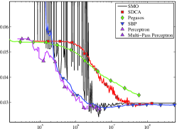
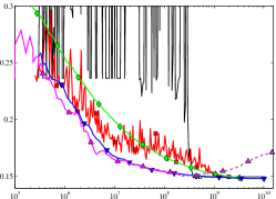
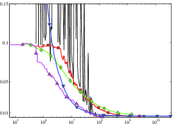
	Kernel Evaluations	Kernel Evaluations	Kernel Evaluations

Figure 2: Classification error on the held-out testing set (linear scale) vs. the number of kernel evaluations performed during optimization (log scale), averaged over ten runs. The Perceptron was run for multiple passes over the data—its curve becomes dashed after the first epoch ($n$ iterations). All algorithms were run for ten epochs, except for Perceptron on Adult, which we ran for $100$ epochs to better illustrate its overfitting.

We first compared the methods on a SVM formulation without an unregularized bias, since Pegasos and SDCA do not naturally handle one. So that this comparison would be implementation-independent, we measure performance in terms of the number of kernel evaluations. As can be seen in Figure 2, the SBP outperforms Pegasos and SDCA, as predicted by the upper bounds. The SMO algorithm has a dramatically different performance profile, in line with the known analysis: it makes relatively little progress, in terms of generalization error, until it reaches a certain critical point, after which it converges rapidly. Unlike the other methods, terminating SMO early in order to obtain a cruder solution does not appear to be advisable.

We also compared to the online Perceptron algorithm. Although use of the Perceptron is justified for non-separable data only if run for a single pass over the training set, we did continue running for multiple passes. The Perceptron’s generalization performance is similar to that of the SBP for the first epoch, but the SBP continues improving over additional passes. As discussed in Section 4.5, the Perceptron is unsafe and might overfit after the first epoch, an effect which is clearly visible on the Adult dataset.

To give a sense of actual runtime, we compared our implementation of the SBP to the SVM package LIBSVM, running on an Intel E7500 processor. We allowed an unregularized bias (since that is what LIBSVM uses), and used the parameters in Table 2. For these experiments, we replaced the Reuters dataset with the version of the Forest dataset used by Nguyen et al. (2010), using their parameters. LIBSVM converged to a solution with $14.9$% error in $195$s on Adult, $0.44$% in $1980$s on MNIST, and $1.8$% in $35$ hours on Forest. In one-quarter of each of these runtimes, SBP obtained $15.0$% error on Adult, $0.46$% on MNIST, and $1.6$% on Forest. These results of course depend heavily on the specific stopping criterion used.

6 Summary and Discussion

The Stochastic Batch Perceptron is a novel approach for training kernelized SVMs. The SBP fares well empirically, and, as summarized in Table 1, our runtime guarantee for the SBP is the best of any existing guarantee for kernelized SVM training. An interesting open question is whether this runtime is optimal, i.e. whether any algorithm relying only on black-box kernel accesses must perform $\Omega\left(((\mathcal{L}^{*}+\epsilon)/\epsilon)^{3}\left\lVert{u}\right\rVert^{4}/\epsilon\right)$ kernel evaluations.

As with other stochastic gradient methods, deciding when to terminate SBP optimization is an open issue. The most practical approach seems to be to terminate when a holdout error stabilizes. We should note that even for methods where the duality gap can be used (e.g. SMO), this criterion is often too strict, and the use of cruder criteria may improve training time.

Acknowledgements:

S. Shalev-Shwartz is supported by the Israeli Science Foundation grant number 590-10.

Appendix A Additional Experiments

	Reuters	Adult	MNIST
Test error
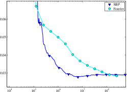
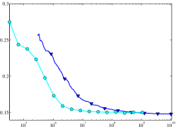
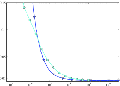
	Inner Products	Inner Products	Inner Products

Figure 3: Classification error on the held-out testing set (linear scale) vs. computational cost measured in units of $d$-dimensional inner products (where the training vectors satisfy $x\in\mathbb{R}^{d}$) (log scale), and averaged over ten runs. For the Fourier features, the computational cost (horizontal axis) is that of computing $k\in\left\{1,2,4,8,\dots\right\}$ pairs of Fourier features over the entire training set, while the test error is that of the optimal classifier trained on the resulting linearized SVM objective.

While our focus in this paper is on optimization of the kernel SVM objective, and not on the broader problem of large-scale learning, one may wonder how well the SBP compares to techniques which accelerate the training of kernel SVMs through approximation. One such is the random Fourier projection algorithm of Rahimi & Recht (2007), which can be used to transform a kernel SVM problem into an approximately-equivalent linear SVM. The resulting problem may then be optimized using one of the many existing fast linear SVM solvers, such as Pegasos, SDCA or SIMBA. Unlike methods (such as the SBP) which rely only on black-box kernel accesses, Rahimi and Recht’s projection technique can only be applied on a certain class of kernel functions (shift-invariant kernels), of which the Gaussian kernel is a member.

For $d$-dimensional feature vectors, and using a Gaussian kernel with parameter $\sigma^{2}$, Rahimi and Recht’s approach is to sample $v_{1},\dots,v_{k}\in\mathbb{R}^{d}$ independently according to $v_{i}\sim\mathcal{N}\left(0,I\right)$, and then define the mapping $\mathcal{P}:\mathbb{R}^{d}\rightarrow\mathbb{R}^{2k}$ as:

$${\mathcal{P}\left(x\right)}_{2i}= \frac{1}{\sqrt{k}}\cos\left(\frac{1}{\sigma}\left\langle{v_{i}},{x}\right\rangle\right)$$

$${\mathcal{P}\left(x\right)}_{2i+1}= \frac{1}{\sqrt{k}}\sin\left(\frac{1}{\sigma}\left\langle{v_{i}},{x}\right\rangle\right)$$

Then $\left\langle{\mathcal{P}\left(x_{i}\right)},{\mathcal{P}\left(x_{j}\right)}\right\rangle\approx K\left(x_{i},x_{j}\right)$, with the quality of this approximation improving with increasing $k$ (see Rahimi & Recht (2007, Claim 1) for details).

Notice that computing each pair of Fourier features requires computing the $d$-dimensional inner product $\left\langle{v},{x}\right\rangle$. For comparison, let us write the Gaussian kernel in the following form:

$$K\left(x_{i},x_{j}\right)= \exp\left(-\frac{1}{2\sigma^{2}}\left\lVert{x_{i}-x_{j}}\right\rVert^{2}\right)$$

$$= \exp\left(-\frac{1}{2\sigma^{2}}\left(\left\lVert{x_{i}}\right\rVert^{2}+\left\lVert{x_{j}}\right\rVert^{2}-2\left\langle{x_{i}},{x_{j}}\right\rangle\right)\right)$$

The norms $\left\lVert{x_{i}}\right\rVert$ may be cheaply precomputed, so the dominant cost of performing a single Gaussian kernel evaluation is, likewise, that of the $d$-dimensional inner product $\left\langle{x_{i}},{x_{j}}\right\rangle$.

This observation suggests that the computational cost of the use of Fourier features may be directly compared with that of a kernel-evaluation-based SVM optimizer in terms of $d$-dimensional inner products. Figure 3 contains such a comparison. In this figure, the computational cost of a $2k$-dimensional Fourier linearization is taken to be the cost of computing $\mathcal{P}\left(x_{i}\right)$ on the entire training set ($kn$ inner products, where $n$ is the number of training examples)—we ignore the cost of optimizing the resulting linear SVM entirely. The plotted testing error is that of the optimum of the resulting linear SVM problem, which approximates the original kernel SVM. We can see that at least on Reuters and MNIST, the SBP is preferable to (i.e. faster than) approximating the kernel with random Fourier features.

Appendix B Implementation Details

$\mbox{{optimize}}\left(n:\mathbb{N},x_{1},\dots,x_{n}:\mathbb{R}^{d},y_{1},\dots,y_{n}:\left\{\pm 1\right\},T_{0}:\mathbb{N},T:\mathbb{N},\nu:\mathbb{R}_{+},K:\mathbb{R}^{d}\times\mathbb{R}^{d}\rightarrow\mathbb{R}_{+}\right)$
1	$\eta_{0}:=1/\sqrt{\max_{i}K\left(x_{i},x_{i}\right)}$;
2	$\alpha^{(0)}:=0^{n}$; $c^{(0)}:=0^{n}$; $r_{0}:=0$;
3	$\mbox{{for }}t:=1\mbox{{ to }}T$
4		$\eta_{t}:=\eta_{0}/\sqrt{t}$;
5		$\gamma:=\mbox{{find\_gamma}}\left(c^{(t-1)},n\nu\right)$;
6		$\mbox{{sample }}i\sim\mbox{{uniform}}\left\{j:c^{(t-1)}_{j}<\gamma\right\}$;
7		$\alpha^{(t)}:=\alpha^{(t-1)}+\eta_{t}e_{i}$;
8		$r_{t}^{2}:=r_{t-1}^{2}+2\eta_{t}c^{(t-1)}_{i}+\eta_{t}^{2}K\left(x_{i},x_{i}\right)$;
9		$\mbox{{for }}j=1\mbox{{ to }}n$
10			$c^{(t)}_{j}:=c^{(t-1)}_{j}+\eta_{t}y_{i}y_{j}K\left(x_{i},x_{j}\right)$;
11		$\mbox{{if }}\left(r_{t}>1\right)\mbox{{ then}}$
12			$\alpha^{(t)}:=\left(1/r_{t}\right)\alpha^{(t)}$; $c^{(t)}:=\left(1/r_{t}\right)c^{(t)}$; $r_{t}:=1$;
13	$\bar{\alpha}:=\frac{1}{T}\sum_{t=1}^{T}\alpha^{(t)}$; $\bar{c}:=\frac{1}{T}\sum_{t=1}^{T}c^{(t)}$; $\gamma:=\mbox{{find\_gamma}}\left(\bar{c},n\nu\right)$;
14	$\mbox{{return }}\bar{\alpha}/\gamma$;

Algorithm 1 Stochastic gradient ascent algorithm for optimizing the kernelized version of Problem 2.3, as described in Section 3.3. Here, $e_{i}$ is the $i$th standard unit basis vector. The find_gamma subroutine finds the “water level” $\gamma$ from the vector of responses $c$ and total volume $n\nu$.

$\mbox{{find\_gamma}}\left(C:\mathbb{R}^{n},n\nu:\mathbb{R}\right)$
1	$lower:=1$; $upper:=n$;
2	$lower\_max:=-\infty$; $lower\_sum:=0$;
3	$\mbox{{while }}lower<upper$
4		$\mbox{{while }}lower<upper$;
5		$middle:=\mbox{{partition}}(C\left[lower:upper\right])$;
6		$middle\_max:=\max\left(lower\_max,C\left[lower:\left(middle-1\right)\right]\right)$;
7		$middle\_sum:=lower\_sum+\sum C\left[lower:\left(middle-1\right)\right]$;
8		$\mbox{{if }}middle\_max\cdot\left(middle-1\right)-middle\_sum\geq n\nu\mbox{{ then}}$
9			$upper:=middle-1$;
10		$else$
11			$lower:=middle$; $lower\_max:=middle\_max$; $lower\_sum:=middle\_sum$;
12	$\mbox{{return }}\left(n\nu-lower\_max\cdot\left(lower-1\right)+lower\_sum\right)/\left(lower-1\right)+lower\_max$;

Algorithm 2 Divide-and-conquer algorithm for finding the “water level” $\gamma$ from an array of responses $C$ and total volume $n\nu$. The partition function chooses a pivot value from the array it receives as an argument (the median would be ideal), places all values less than the pivot at the start of the array, all values greater at the end, and returns the index of the pivot in the resulting array.

We begin this appendix by providing complete pseudo-code, which may be found in Algorithm 1, for the SBP algorithm which we outlined in Section 3.4. This implementation requires that we be able to find a minimax-optimal probability distribution $p^{*}$ to the objective of Equation 3.1.

As was discussed in Section 3.2, in a problem without an unregularized bias, such a probability distribution can be derived from the “water level” $\gamma$, which can be found in $O(n)$ time using Algorithm 2. This algorithm works by subdividing the set of responses into those less than, equal to and greater than a pivot value (if one uses the median, which can be found in linear time using e.g. the median-of-medians algorithm (Blum et al., 1973), then the overall will be linear in $n$). Then, it calculates the size, minimum and sum of each of these subsets, from which the total volume of the water required to cover the subsets can be easily calculated. It then recurses into the subset containing the point at which a volume of $n\nu$ just suffices to cover the responses, and continues until $\gamma$ is found.

Figure 4: Illustration of how one finds the “water level” in a problem with an unregularized bias. The two curves represent the heights of two basins of heights $c_{i}-b$ and $c_{i}+b$, corresponding to the negative and positive examples, respectively, with the bias $b$ determining the relative heights of the basins. Optimizing over $\xi$ and $p$ corresponds to filling these two basins with water of total volume $n\nu$ and common water level $\gamma$, while optimizing $b$ corresponds to ensuring that water covers the same number of indices in each basin.

$\mbox{{find\_gamma\_and\_bias}}\left(y:\left\{\pm 1\right\}^{n},C:\mathbb{R}^{n},n\nu:\mathbb{R}\right)$
1	$C^{+}:=\{C[i]:y[i]=+1\}$; $n^{+}:=\left\lvert{C^{+}}\right\rvert$; $lower^{+}:=1$; $upper^{+}:=n^{+}$; $lower\_max^{+}:=-\infty$; $lower\_sum^{+}:=0$;
2	$C^{-}:=\{C[i]:y[i]=-1\}$; $n^{-}:=\left\lvert{C^{-}}\right\rvert$; $lower^{-}:=1$; $upper^{-}:=n^{-}$; $lower\_max^{-}:=-\infty$; $lower\_sum^{-}:=0$;
3	$middle^{+}:=\mbox{{partition}}(C^{+}\left[lower^{+}:upper^{+}\right])$;
4	$middle^{-}:=\mbox{{partition}}(C^{-}\left[lower^{-}:upper^{-}\right])$;
5	$middle\_max^{+}:=\max\left(C\left[lower^{+}:\left(middle^{+}-1\right)\right]\right)$; $middle\_sum^{+}:=\sum C\left[lower^{+}:\left(middle^{+}-1\right)\right]$;
6	$middle\_max^{-}:=\max\left(C\left[lower^{-}:\left(middle^{-}-1\right)\right]\right)$; $middle\_sum^{-}:=\sum C\left[lower^{-}:\left(middle^{-}-1\right)\right]$;
7	$\mbox{{while }}\left(lower^{+}<upper^{+}\right)\mbox{{ or }}\left(lower^{-}<upper^{-}\right)$
8		$direction^{+}:=0$; $direction^{-}:=0$;
9		$\mbox{{if }}middle^{+}<lower^{-}\mbox{{ then }}direction^{+}=1$;
10		$\mbox{{else if }}middle^{+}>upper^{-}\mbox{{ then }}direction^{+}=-1$;
11		$\mbox{{if }}middle^{-}<lower^{+}\mbox{{ then }}direction^{-}=1$;
12		$\mbox{{else if }}middle^{-}>upper^{+}\mbox{{ then }}direction^{-}=-1$;
13		$\mbox{{if }}direction^{+}=direction^{-}=0\mbox{{ then}}$
14			$volume^{+}:=middle\_max^{+}\cdot\left(middle^{+}-1\right)-middle\_sum^{+}$;
15			$volume^{-}:=middle\_max^{-}\cdot\left(middle^{-}-1\right)-middle\_sum^{-}$;
16			$\mbox{{if }}volume^{+}+volume^{-}\geq n\nu\mbox{{ then}}$
17				$\mbox{{if }}middle^{+}>middle^{-}\mbox{{ then }}direction^{+}=-1$;
18				$\mbox{{else if }}middle^{-}>middle^{+}\mbox{{ then }}direction^{-}=-1$;
19				$\mbox{{else if }}upper^{+}-lower^{+}>upper^{-}-lower^{-}\mbox{{ then }}direction^{+}=-1$;
20				$\mbox{{else }}direction^{-}=-1$;
21			else
22				$\mbox{{if }}middle^{+}<middle^{-}\mbox{{ then }}direction^{+}=1$;
23				$\mbox{{else if }}middle^{-}<middle^{+}\mbox{{ then }}direction^{-}=1$;
24				$\mbox{{else if }}upper^{+}-lower^{+}>upper^{-}-lower^{-}\mbox{{ then }}direction^{+}=1$;
25				$\mbox{{else }}direction^{-}=1$;
26		$\mbox{{if }}direction^{+}\neq 0\mbox{{ then}}$
27			$\mbox{{if }}direction^{+}>0\mbox{{ then }}upper^{+}:=middle^{+}-1$;
28			$\mbox{{else }}lower^{+}:=middle^{+}$; $lower\_max^{+}:=middle\_max^{+}$; $lower\_sum^{+}:=middle\_sum^{+}$;
29			$middle^{+}:=\mbox{{partition}}(C^{+}\left[lower^{+}:upper^{+}\right])$;
30			$middle\_max^{+}:=\max\left(lower\_max^{+},C\left[lower^{+}:\left(middle^{+}-1\right)\right]\right)$;
31			$middle\_sum^{+}:=lower\_sum^{+}+\sum C\left[lower^{+}:\left(middle^{+}-1\right)\right]$;
32		$\mbox{{if }}direction^{-}\neq 0\mbox{{ then}}$
33			$\mbox{{if }}direction^{-}>0\mbox{{ then }}upper^{-}:=middle^{-}-1$;
34			$\mbox{{else }}lower^{-}:=middle^{-}$; $lower\_max^{-}:=middle\_max^{-}$; $lower\_sum^{-}:=middle\_sum^{-}$;
35			$middle^{-}:=\mbox{{partition}}(C^{-}\left[lower^{-}:upper^{-}\right])$;
36			$middle\_max^{-}:=\max\left(lower\_max^{-},C\left[lower^{-}:\left(middle^{-}-1\right)\right]\right)$;
37			$middle\_sum^{-}:=lower\_sum^{-}+\sum C\left[lower^{-}:\left(middle^{-}-1\right)\right]$;
38	// at this point $lower^{+}=lower^{-}=upper^{+}=upper^{-}$
39	$\Delta\gamma:=\left(n\nu+lower\_sum^{+}+lower\_sum^{-}\right)/\left(lower^{+}-1\right)-lower\_max^{+}-lower\_max^{-}$;
40	$\mbox{{if }}lower^{+}<n^{+}\mbox{{ then }}\Delta\gamma^{+}:=\min\left(\Delta\gamma,C^{+}[lower^{+}]-lower\_max^{+}\right)\mbox{{ else }}\Delta\gamma^{+}:=\Delta\gamma$;
41	$\mbox{{if }}lower^{-}<n^{-}\mbox{{ then }}\Delta\gamma^{-}:=\min\left(\Delta\gamma,C^{-}[lower^{-}]-lower\_max^{-}\right)\mbox{{ else }}\Delta\gamma^{-}:=\Delta\gamma$;
42	$\gamma^{+}:=lower\_max^{+}+0.5\cdot\left(\Delta\gamma+\Delta\gamma^{+}-\Delta\gamma^{-}\right)$; $\gamma^{-}:=lower\_max^{-}+0.5\cdot\left(\Delta\gamma-\Delta\gamma^{+}+\Delta\gamma^{-}\right)$;
43	$\gamma:=0.5\cdot\left(\gamma^{+}+\gamma^{-}\right)$; $b:=0.5\cdot\left(\gamma^{-}-\gamma^{+}\right)$;
44	$\mbox{{return }}\left(\gamma,b\right)$;

Algorithm 3 Divide-and-conquer algorithm for finding the “water level” $\gamma$ and bias $b$ from an array of labels $y$, array of responses $C$ and total volume $n\nu$, for a problem with an unregularized bias. The partition function is as in Algorithm 2.

In Section 3.6, we mentioned that a similar result holds for the objective of Equation 3.9, which adds an unregularized bias.

As before, finding the water level $\gamma$ reduces to finding minimax-optimal values of $p^{*}$, $\xi^{*}$ and $b^{*}$. The characterization of such solutions is similar to that in the case without an unregularized bias. In particular, for a fixed value of $b$, we may still think about “pouring water into a basin”, except that the height of the basin is now $c_{i}+y_{i}b$, rather than $c_{i}$.

When $b$ is not fixed it is easier to think of two basins, one containing the positive examples, and the other the negative examples. These basins will be filled with water of a total volume of $n\nu$, to a common water level $\gamma$. The relative heights of the two basins are determined by $b$: increasing $b$ will raise the basin containing the positive examples, while lowering that containing the negative examples by the same amount. This is illustrated in Figure 4.

It remains only to determine what characterizes a minimax-optimal value of $b$. Let $k^{+}$ and $k^{-}$ be the number of elements covered by water in the positive and negative basins, respectively, for some $b$. If $k^{+}>k^{-}$, then raising the positive basin and lowering the negative basin by the same amount (i.e. increasing $b$) will raise the overall water level, showing that $b$ is not optimal. Hence, for an optimal $b$, water must cover an equal number of indices in each basin. Similar reasoning shows that an optimal $p^{*}$ must place equal probability mass on each of the two classes.

Once more, the resulting problem is amenable to a divide-and-conquer approach. The water level $\gamma$ and bias $b$ will be found in $O(n)$ time by Algorithm 3, provided that the partition function chooses the median as the pivot.

Appendix C Proofs of Lemmas 3.1 and 3.2

Lemma 3.1.

For any $w$, let $p^{*},\xi^{*}$ be minimax optimal for Equation 3.1. Then $\sum_{i=1}^{n}p^{*}_{i}y_{i}\Phi\left(x_{i}\right)$ is a supergradient of $f(w)$ at $w$.

Proof.

By the definition of $f$, for any $v\in\mathbb{R}^{d}$:

$$f\left(w+v\right)=$$

$$\max_{\xi\succeq 0,\mathbf{1}^{T}\xi\leq n\nu}\min_{p\in\Delta^{n}}\sum_{i=1}^{n}p_{i}\left(y_{i}\left\langle{w+v},{\Phi\left(x_{i}\right)}\right\rangle+\xi_{i}\right)$$

Substituting the particular value $p^{*}$ for $p$ can only increase the RHS, so:

$$f\left(w+v\right)\leq \max_{\xi\succeq 0,\mathbf{1}^{T}\xi\leq n\nu}\sum_{i=1}^{n}p^{*}_{i}\left(y_{i}\left\langle{w+v},{\Phi\left(x_{i}\right)}\right\rangle+\xi_{i}\right)$$

$$\leq \max_{\xi\succeq 0,\mathbf{1}^{T}\xi\leq n\nu}\sum_{i=1}^{n}p^{*}_{i}\left(y_{i}\left\langle{w},{\Phi\left(x_{i}\right)}\right\rangle+\xi_{i}\right)$$

$$+\sum_{i=1}^{n}p^{*}_{i}y_{i}\left\langle{v},{\Phi\left(x_{i}\right)}\right\rangle$$

Because $p^{*}$ is minimax-optimal at $w$:

$$f\left(w+v\right)\leq f\left(w\right)+\sum_{i=1}^{n}p^{*}_{i}y_{i}\left\langle{v},{\Phi\left(x_{i}\right)}\right\rangle$$

$$\leq f\left(w\right)+\left\langle{v},{\sum_{i=1}^{n}p^{*}_{i}y_{i}\Phi\left(x_{i}\right)}\right\rangle$$

So $\sum_{i=1}^{n}p^{*}_{i}y_{i}\Phi\left(x_{i}\right)$ is a supergradient of $f$. ∎

Lemma 3.2.

For any $T,\delta>0$, after $T$ iterations of the Stochastic Batch Perceptron, with probability at least $1-\delta$, the average iterate $\bar{w}=\frac{1}{T}\sum_{t=1}^{T}w^{(t)}$ (corresponding to $\bar{\alpha}=\frac{1}{T}\sum_{t=1}^{T}\alpha^{(t)}$), satisfies: $f\left(\bar{w}\right)\geq\sup_{\left\lVert{w}\right\rVert\leq 1}f\left(w\right)-O\left(\sqrt{\frac{1}{T}\log\frac{1}{\delta}}\right).$

Proof.

Define $h=-\frac{1}{r}f$, where $f$ is as in Equation 3.1. Then the stated update rules constitute an instance of Zinkevich’s algorithm, in which steps are taken in the direction of stochastic subgradients $g^{(t)}$ of $h$ at $w^{(t)}=\sum_{i=1}^{n}\alpha_{i}y_{i}\Phi\left(x_{i}\right)$.

The claimed result follows directly from Zinkevich (2003, Theorem 1) combined with an online-to-batch conversion analysis in the style of Cesa-Bianchi et al. (2001, Lemma 1). ∎

Appendix D Data-Laden Analyses

We’ll begin by presenting a bound on the sample size $n$ required to guarantee good generalization performance (in terms of the 0/1 loss) for a classifier which is $\epsilon$-suboptimal in terms of the empirical hinge loss. The following result, which follows from Srebro et al. (2010, Theorem 1), is a vital building block of the bounds derived in the remainder of this appendix:

Lemma D.1.

Consider the expected 0/1 and hinge losses:

$$\mathcal{L}_{0/1}\left(w\right) =\mathbb{E}_{x,y}\left[\mathbf{1}_{y\left\langle{w},{x}\right\rangle\leq 0}\right]$$

$$\mathcal{L}\left(w\right) =\mathbb{E}_{x,y}\left[\max\left(0,1-y\left\langle{w},{x}\right\rangle\right)\right]$$

Let $u$ be an arbitrary linear classifier, and suppose that we sample a training set of size $n$, with $n$ given by the following equation, for parameters $B\geq\left\lVert{u}\right\rVert$, $\epsilon>0$ and $\delta\in\left(0,1\right)$:

$$n=\tilde{O}\left(\left(\frac{\mathcal{L}\left(u\right)+\epsilon}{\epsilon}\right)\frac{\left(B+\sqrt{\log\frac{1}{\delta}}\right)^{2}+rB\log\frac{1}{\delta}}{\epsilon}\right)$$ (D.1)

where $r\geq\left\lVert{x}\right\rVert$ is an upper bound on the radius of the data. Then, with probability $1-\delta$ over the i.i.d. training sample $x_{i},y_{i}:i\in\left\{1,\dots,n\right\}$, uniformly for all linear classifiers $w$ satisfying:

$$\left\lVert{w}\right\rVert \leq B$$

$$\hat{\mathcal{L}}\left(w\right)-\hat{\mathcal{L}}\left(u\right) \leq\epsilon$$

where $\hat{\mathcal{L}}$ is the empirical hinge loss:

$$\hat{\mathcal{L}}\left(w\right)=\frac{1}{n}\sum_{i=1}^{n}\max\left(0,1-y_{i}\left\langle{w},{x_{i}}\right\rangle\right)\\$$

we have that:

$$\hat{\mathcal{L}}\left(u\right) \leq\mathcal{L}\left(u\right)+\epsilon$$

$$\mathcal{L}_{0/1}\left(w\right) \leq\hat{\mathcal{L}}\left(u\right)+\epsilon$$

and in particular that:

$$\mathcal{L}_{0/1}\left(w\right)\leq\mathcal{L}\left(u\right)+2\epsilon$$

In the remainder of this appendix, we will apply the above result to derive generalization bounds on the performance of the various algorithms under consideration, in the data-laden setting.

D.1 Stochastic Batch Perceptron

We will here present a more careful derivation of the main result of Section 3.5, bounding the generalization performance of the SBP.

Theorem D.2.

Let $u$ be an arbitrary linear classifier in the RKHS, let $\epsilon>0$ be given, and suppose that $K\left(x,x\right)\leq r^{2}$ with probability $1$. There exist values of the training size $n$, iteration count $T$ and parameter $\nu$ such that Algorithm 1 finds a solution $w=\sum_{i=1}^{n}\alpha_{i}y_{i}\Phi\left(x_{i}\right)$ satisfying:

$$\mathcal{L}_{0/1}\left(w\right)\leq\mathcal{L}\left(u\right)+\epsilon$$

where $\mathcal{L}_{0/1}$ and $\mathcal{L}$ are the expected 0/1 and hinge losses, respectively, after performing the following number of kernel evaluations:

$$\mbox{\#K}=\tilde{O}\left(\left(\frac{\mathcal{L}\left(u\right)+\epsilon}{\epsilon}\right)^{3}\frac{r^{3}\left\lVert{u}\right\rVert^{4}}{\epsilon}\log^{2}\frac{1}{\delta}\right)$$

with the size of the support set of $w$ (the number nonzero elements in $\alpha$) satisfying:

$$\mbox{\#S}=O\left(\left(\frac{\mathcal{L}\left(u\right)+\epsilon}{\epsilon}\right)^{2}r^{2}\left\lVert{u}\right\rVert^{2}\log\frac{1}{\delta}\right)$$

the above statements holding with probability $1-\delta$.

Proof.

For a training set of size $n$, where:

$$n=\tilde{O}\left(\left(\frac{\mathcal{L}\left(u\right)+\epsilon}{\epsilon}\right)\frac{rB^{2}}{\epsilon}\log\frac{1}{\delta}\right)$$

taking $B=2\left\lVert{u}\right\rVert$ in Lemma D.1 gives that $\hat{\mathcal{L}}\left(u\right)\leq\mathcal{L}\left(u\right)+\epsilon$ and $\mathcal{L}_{0/1}\left(w\right)\leq\mathcal{L}\left(u\right)+2\epsilon$ with probability $1-\delta$ over the training sample, uniformly for all linear classifiers $w$ such that $\left\lVert{w}\right\rVert\leq B$ and $\hat{\mathcal{L}}\left(w\right)-\hat{\mathcal{L}}\left(u\right)\leq\epsilon$, where $\hat{\mathcal{L}}$ is the empirical hinge loss. We will now show that these inequalities are satisfied by the result of Algorithm 1. Define:

$$\hat{w}^{*}=\underset{w:\left\lVert{w}\right\rVert\leq\left\lVert{u}\right\rVert}{\mathrm{argmin}}\>\hat{\mathcal{L}}\left(w\right)$$

Because $\hat{w}^{*}$ is a Pareto optimal solution of the bi-criterion objective of Problem 2.1, if we choose the parameter $\nu$ to the slack-constrained objective (Problem 2.3) such that $\left\lVert{\hat{w}^{*}}\right\rVert\nu=\hat{\mathcal{L}}\left(\hat{w}^{*}\right)$, then the optimum of the slack-constrained objective will be equivalent to $\hat{w}^{*}$ (Lemma 2.1). As was discussed in Section 3.5, We will use Lemma 3.2 to find the number of iterations $T$ required to satisfy Equation 3.7 (with $u=\hat{w}^{*}$). This yields that, if we perform $T$ iterations of Algorithm 1, where $T$ satisfies the following:

$$T\geq O\left(\left(\frac{\hat{\mathcal{L}}\left(\hat{w}^{*}\right)+\epsilon}{\epsilon}\right)^{2}r^{2}\left\lVert{\hat{w}^{*}}\right\rVert^{2}\log\frac{1}{\delta}\right)$$ (D.2)

then the resulting solution $w=\bar{w}/\gamma$ will satisfy:

$$\left\lVert{w}\right\rVert \leq 2\left\lVert{\hat{w}^{*}}\right\rVert$$

$$\hat{\mathcal{L}}\left(w\right)-\hat{\mathcal{L}}\left(\hat{w}^{*}\right) \leq\epsilon$$

with probability $1-\delta$. That is:

$$\left\lVert{w}\right\rVert \leq 2\left\lVert{\hat{w}^{*}}\right\rVert$$

$$\leq B$$

and:

$$\hat{\mathcal{L}}\left(w\right) \leq\hat{\mathcal{L}}\left(\hat{w}^{*}\right)+\epsilon$$

$$\leq\hat{\mathcal{L}}\left(u\right)+\epsilon$$

These are precisely the bounds on $\left\lVert{w}\right\rVert$ and $\hat{\mathcal{L}}\left(w\right)$ which we determined (at the start of the proof) to be necessary to permit us to apply Lemma D.1. Each of the $T$ iterations requires $n$ kernel evaluations, so the product of the bounds on $T$ and $n$ bounds the number of kernel evaluations (we may express Equation D.2 in terms of $\mathcal{L}\left(u\right)$ and $\left\lVert{u}\right\rVert$ instead of $\hat{\mathcal{L}}\left(\hat{w}^{*}\right)$ and $\left\lVert{\hat{w}^{*}}\right\rVert$, since $\hat{\mathcal{L}}\left(\hat{w}^{*}\right)\leq\hat{\mathcal{L}}\left(u\right)\leq\mathcal{L}\left(u\right)+\epsilon$ and $\left\lVert{\hat{w}^{*}}\right\rVert\leq\left\lVert{u}\right\rVert$).

Because each iteration will add at most one new element to the support set, the size of the support set is bounded by the number of iterations, $T$.

This discussion has proved that we can achieve suboptimality $2\epsilon$ with probability $1-2\delta$ with the given #K and #S. Because scaling $\epsilon$ and $\delta$ by $1/2$ only changes the resulting bounds by constant factors, these results apply equally well for suboptimality $\epsilon$ with probability $1-\delta$. ∎

D.2 Pegasos / SGD on $\hat{\mathcal{L}}$

If $w$ is the result of a call to the Pegasos algorithm (Shalev-Shwartz et al., 2011) without a projection step, then the analysis of Kakade & Tewari (2009, Corollary 7) permits us to bound the suboptimality relative to an arbitrary reference classifier $u$, with probability $1-\delta$, as:

$$\left(\frac{\lambda}{2}\left\lVert{w}\right\rVert^{2}+\hat{\mathcal{L}}\left(w\right)\right)-\left(\frac{\lambda}{2}\left\lVert{u}\right\rVert^{2}+\hat{\mathcal{L}}\left(u\right)\right)\leq$$ (D.3)

$$\frac{84r^{2}\log T}{\lambda T}\log\frac{1}{\delta}$$

Equation D.3 implies that, if one performs the following number of iterations, then the resulting solution will be $\epsilon/2$-suboptimal in the regularized objective, with probability $1-\delta$:

$$T=\tilde{O}\left(\frac{1}{\epsilon}\cdot\frac{r^{2}}{\lambda}\log\frac{1}{\delta}\right)$$

Here, $\epsilon$ bounds the suboptimality not of the empirical hinge loss, but rather of the regularized objective (hinge loss + regularization). Although the dependence on $1/\epsilon$ is linear, accounting for the $\lambda$ dependence results in a bound which is not nearly good as the above appears. To see this, we’ll follow Shalev-Shwartz & Srebro (2008) by decomposing the suboptimality in the empirical hinge loss as:

$$\hat{\mathcal{L}}\left(w\right)-\hat{\mathcal{L}}\left(u\right) =\frac{\epsilon}{2}-\frac{\lambda}{2}\left\lVert{w}\right\rVert^{2}+\frac{\lambda}{2}\left\lVert{u}\right\rVert^{2}$$

$$\leq\frac{\epsilon}{2}+\frac{\lambda}{2}\left\lVert{u}\right\rVert^{2}$$

In order to have both terms bounded by $\epsilon/2$, we choose $\lambda=\epsilon/\left\lVert{u}\right\rVert^{2}$, which reduces the RHS of the above to $\epsilon$. Continuing to use this choice of $\lambda$, we next decompose the squared norm of $w$ as:

$$\frac{\lambda}{2}\left\lVert{w}\right\rVert^{2} =\frac{\epsilon}{2}-\hat{\mathcal{L}}\left(w\right)+\hat{\mathcal{L}}\left(u\right)+\frac{\lambda}{2}\left\lVert{u}\right\rVert^{2}$$

$$\leq\frac{\epsilon}{2}+\hat{\mathcal{L}}\left(u\right)+\frac{\lambda}{2}\left\lVert{u}\right\rVert^{2}$$

$$\left\lVert{w}\right\rVert^{2} \leq 2\left(\frac{\hat{\mathcal{L}}\left(u\right)+\epsilon}{\epsilon}\right)\left\lVert{u}\right\rVert^{2}$$

Hence, we will have that:

$$\left\lVert{w}\right\rVert^{2} \leq 2\left(\frac{\hat{\mathcal{L}}\left(u\right)+\epsilon}{\epsilon}\right)\left\lVert{u}\right\rVert^{2}$$ (D.4)

$$\hat{\mathcal{L}}\left(w\right)-\hat{\mathcal{L}}\left(u\right) \leq\epsilon$$

with probability $1-\delta$, after performing the following number of iterations:

$$T=\tilde{O}\left(\frac{r^{2}\left\lVert{u}\right\rVert^{2}}{\epsilon^{2}}\log\frac{1}{\delta}\right)$$ (D.5)

There are two ways in which we will use this bound on $T$ to find bound on the number of kernel evaluations required to achieve some desired regularization error. The easiest is to note that the bound of Equation D.5 exceeds that of Lemma D.1, so that if we take $T=n$, then with high probability, we’ll achieve generalization error $2\epsilon$ after $Tn=T^{2}$ kernel evaluations:

$$\mbox{\#K}=\tilde{O}\left(\frac{r^{4}\left\lVert{u}\right\rVert^{4}}{\epsilon^{4}}\log^{2}\frac{1}{\delta}\right)$$ (D.6)

Because we take the number of iterations to be precisely the same as the number of training examples, this is essentially the online stochastic setting.

Alternatively, we may combine our bound on $T$ with Lemma D.1. This yields the following bound on the generalization error of Pegasos in the data-laden batch setting.

Theorem D.3.

Let $u$ be an arbitrary linear classifier in the RKHS, let $\epsilon>0$ be given, and suppose that $K\left(x,x\right)\leq r^{2}$ with probability $1$. There exist values of the training size $n$, iteration count $T$ and parameter $\nu$ such that kernelized Pegasos finds a solution $w=\sum_{i=1}^{n}\alpha_{i}y_{i}\Phi\left(x_{i}\right)$ satisfying:

$$\mathcal{L}_{0/1}\left(w\right)\leq\mathcal{L}\left(u\right)+\epsilon$$

where $\mathcal{L}_{0/1}$ and $\mathcal{L}$ are the expected 0/1 and hinge losses, respectively, after performing the following number of kernel evaluations:

$$\mbox{\#K}=\tilde{O}\left(\left(\frac{\mathcal{L}\left(u\right)+\epsilon}{\epsilon}\right)^{2}\frac{r^{3}\left\lVert{u}\right\rVert^{4}}{\epsilon^{3}}\log^{2}\frac{1}{\delta}\right)$$

with the size of the support set of $w$ (the number nonzero elements in $\alpha$) satisfying:

$$\mbox{\#S}=\tilde{O}\left(\frac{r^{2}\left\lVert{u}\right\rVert^{2}}{\epsilon^{2}}\log\frac{1}{\delta}\right)$$

the above statements holding with probability $1-\delta$.

Proof.

Same proof technique as in Theorem D.2. ∎

Because of the extra term in the bound on $\left\lVert{w}\right\rVert$ in Equation D.4, theorem D.3 gives a bound which is worse by a factor of $\left(\mathcal{L}\left(u\right)+\epsilon\right)/\epsilon$ than what we might have hoped to recover. When $\epsilon\ll\mathcal{L}\left(u\right)$, this extra factor results in the bound going as $1/\epsilon^{5}$ rather than $1/\epsilon^{4}$. We need to use Equation D.6 to get a $1/\epsilon^{4}$ bound in this case.

Although this bound on the generalization performance of Pegasos is not quite what we expected, for the related algorithm which performs SGD on the following objective:

$$\min_{w\in\mathbb{R}^{d}} \frac{1}{n}\sum_{i=1}^{n}\ell\left(y_{i}\left\langle{w},{\Phi\left(x_{i}\right)}\right\rangle\right)$$

subject to: $$\left\lVert{w}\right\rVert^{2}\leq B^{2}$$

the same proof technique yields the desired bound (i.e. without the extra $\left(\mathcal{L}\left(u\right)+\epsilon\right)/\epsilon$ factor). This is the origin of the “SGD on $\hat{\mathcal{L}}$” row in Table 1.

D.3 Perceptron

Analysis of the venerable online Perceptron algorithm is typically presented as a bound on the number of mistakes made by the algorithm in terms of the hinge loss of the best classifier—this is precisely the form which we consider in this document, despite the fact that the online Perceptron does not optimize any scalarization of the bi-criterion SVM objective of Problem 2.1. Interestingly, the performance of the Perceptron matches that of the SBP, as is shown in the following theorem:

Theorem D.4.

Let $u$ be an arbitrary linear classifier in the RKHS, let $\epsilon>0$ be given, and suppose that $K\left(x,x\right)\leq r^{2}$ with probability $1$. There exists a value of the training size $n$ such that when the Perceptron algorithm is run for a single “pass” over the dataset, the result is a solution $w=\sum_{i=1}^{n}\alpha_{i}y_{i}\Phi\left(x_{i}\right)$ satisfying:

$$\mathcal{L}_{0/1}\left(w\right)\leq\mathcal{L}\left(u\right)+\epsilon$$

where $\mathcal{L}_{0/1}$ and $\mathcal{L}$ are the expected 0/1 and hinge losses, respectively, after performing the following number of kernel evaluations:

$$\mbox{\#K}=\tilde{O}\left(\left(\frac{\mathcal{L}\left(u\right)+\epsilon}{\epsilon}\right)^{3}\frac{r^{4}\left\lVert{u}\right\rVert^{4}}{\epsilon}\frac{1}{\delta}\right)$$

with the size of the support set of $w$ (the number nonzero elements in $\alpha$) satisfying:

$$\mbox{\#S}=O\left(\left(\frac{\mathcal{L}\left(u\right)+\epsilon}{\epsilon}\right)^{2}r^{2}\left\lVert{u}\right\rVert^{2}\frac{1}{\delta}\right)$$

the above statements holding with probability $1-\delta$.

Proof.

If we run the online Perceptron algorithm for a single pass over the dataset, then Corollary 5 of (Shalev-Shwartz, 2007) gives the following mistake bound, for $\mathcal{M}$ being the set of iterations on which a mistake is made:

$$\left\lvert{\mathcal{M}}\right\rvert\leq\sum_{i\in\mathcal{M}}\ell\left(y_{i}\left\langle{u},{\Phi\left(x_{i}\right)}\right\rangle\right)$$ (D.7)

$$+r\left\lVert{u}\right\rVert\sqrt{\sum_{i\in\mathcal{M}}\ell\left(y_{i}\left\langle{u},{\Phi\left(x_{i}\right)}\right\rangle\right)}+r^{2}\left\lVert{u}\right\rVert^{2}$$

$$\sum_{i=1}^{n}\ell_{0/1}\left(y_{i}\left\langle{w_{i}},{\Phi\left(x_{i}\right)}\right\rangle\right)\leq\sum_{i=1}^{n}\ell\left(y_{i}\left\langle{u},{\Phi\left(x_{i}\right)}\right\rangle\right)+$$

$$+r\left\lVert{u}\right\rVert\sqrt{\sum_{i=1}^{n}\ell\left(y_{i}\left\langle{u},{\Phi\left(x_{i}\right)}\right\rangle\right)}+r^{2}\left\lVert{u}\right\rVert^{2}$$

Here, $\ell$ is the hinge loss and $\ell_{0/1}$ is the 0/1 loss. Dividing through by $n$:

$$\frac{1}{n}\sum_{i=1}^{n}\ell_{0/1}\left(y_{i}\left\langle{w_{i}},{\Phi\left(x_{i}\right)}\right\rangle\right)\leq\frac{1}{n}\sum_{i=1}^{n}\ell\left(y_{i}\left\langle{u},{\Phi\left(x_{i}\right)}\right\rangle\right)$$

$$+\frac{r\left\lVert{u}\right\rVert}{\sqrt{n}}\sqrt{\frac{1}{n}\sum_{i=1}^{n}\ell\left(y_{i}\left\langle{u},{\Phi\left(x_{i}\right)}\right\rangle\right)}+\frac{r^{2}\left\lVert{u}\right\rVert^{2}}{n}$$

If we suppose that the $x_{i},y_{i}$s are i.i.d., and that $w\sim\mbox{Unif}\left(w_{1},\dots,w_{n}\right)$ (this is a “sampling” online-to-batch conversion), then:

$$\mathbb{E}\left[\mathcal{L}_{0/1}\left(w\right)\right]\leq\mathcal{L}\left(u\right)+\frac{r\left\lVert{u}\right\rVert}{\sqrt{n}}\sqrt{\mathcal{L}\left(u\right)}+\frac{r^{2}\left\lVert{u}\right\rVert^{2}}{n}$$

Hence, the following will be satisfied:

$$\mathbb{E}\left[\mathcal{L}_{0/1}\left(w\right)\right]\leq\mathcal{L}\left(u\right)+\epsilon$$ (D.8)

when:

$$n\leq O\left(\left(\frac{\mathcal{L}\left(u\right)+\epsilon}{\epsilon}\right)\frac{r^{2}\left\lVert{u}\right\rVert^{2}}{\epsilon}\right)$$

The expectation is taken over the random sampling of $w$. The number of kernel evaluations performed by the $i$th iteration of the Perceptron will be equal to the number of mistakes made before iteration $i$. This quantity is upper bounded by the total number of mistakes made over $n$ iterations, which is given by the mistake bound of equation D.7:

$$\left\lvert{\mathcal{M}}\right\rvert\leq n\mathcal{L}\left(u\right)+r\left\lVert{u}\right\rVert\sqrt{n\mathcal{L}\left(u\right)}+r^{2}\left\lVert{u}\right\rVert^{2}$$

$$\leq O\left(\left(\frac{1}{\epsilon}\left(\frac{\mathcal{L}\left(u\right)+\epsilon}{\epsilon}\right)\mathcal{L}\left(u\right)\right.\right.$$

$$+\left.\left.\sqrt{\frac{1}{\epsilon}\left(\frac{\mathcal{L}\left(u\right)+\epsilon}{\epsilon}\right)\mathcal{L}\left(u\right)}+1\right)r^{2}\left\lVert{u}\right\rVert^{2}\right)$$

$$\leq O\left(\left(\left(\frac{\mathcal{L}\left(u\right)+\epsilon}{\epsilon}\right)^{2}-\left(\frac{\mathcal{L}\left(u\right)+\epsilon}{\epsilon}\right)\right.\right.$$

$$\left.+\sqrt{\left(\frac{\mathcal{L}\left(u\right)+\epsilon}{\epsilon}\right)^{2}-\left(\frac{\mathcal{L}\left(u\right)+\epsilon}{\epsilon}\right)}+1\right)$$

$$\left.\cdot r^{2}\left\lVert{u}\right\rVert^{2}\right)$$

$$\leq O\left(\left(\frac{\mathcal{L}\left(u\right)+\epsilon}{\epsilon}\right)^{2}r^{2}\left\lVert{u}\right\rVert^{2}\right)$$

The number of mistakes $\left\lvert{\mathcal{M}}\right\rvert$ is necessarily equal to the size of the support set of the resulting classifier. Substituting this bound into the number of iterations:

$$\mbox{\#K}= n\left\lvert{\mathcal{M}}\right\rvert$$

$$\leq O\left(\left(\frac{\mathcal{L}\left(u\right)+\epsilon}{\epsilon}\right)^{3}\frac{r^{4}\left\lVert{u}\right\rVert^{4}}{\epsilon}\right)$$

This holds in expectation, but we can turn this into a high-probability result using Markov’s inequality, resulting in in a $\delta$-dependence of $\frac{1}{\delta}$. ∎

Although this result has a $\delta$-dependence of $1/\delta$, this is merely a relic of the simple online-to-batch conversion which we use in the analysis. Using a more complex algorithm (e.g. Cesa-Bianchi et al. (2001)) would likely improve this term to $\log\frac{1}{\delta}$.

Appendix E Convergence rates of dual optimization methods

In this section we discuss existing analyses of dual optimization methods. We first underscore possible gaps between dual sub-optimality and primal sub-optimality. Therefore, to relate existing analyzes in the literature of the dual sub-optimality, we must find a way to connect between the dual sub-optimality and primal sub-optimality. We do so using a result due to Scovel et al. (2008), and based on this result, we derive convergence rates on the primal sub-optimality.

Throughout this section, the “SVM problem” is taken to be the regularized objective of Problem 2.2. We denote the primal objective by:

$$P(w)=\frac{\lambda}{2}\|w\|^{2}+\frac{1}{n}\sum_{i=1}^{n}\ell(y_{i}\left\langle{w,x_{i}},{)}\right\rangle$$

The dual objective can be written as:

$$D(\alpha)={\lambda}\left(\sum_{i=1}^{n}\alpha_{i}-\frac{1}{2}\sum_{i,j=1}^{n}\alpha_{i}\alpha_{j}Q_{ij}\right)$$

where $Q_{ij}=y_{i}y_{j}\left\langle{x_{i}},{x_{j}}\right\rangle$, and the dual constraints are $\alpha\in[0,1/(\lambda n)]^{n}$. Finally, by strong duality we have:

$$P^{*}=\arg\max_{w}P(w)=\underset{\alpha\in[0,1/(\lambda n)]^{n}}{\mathrm{argmax}}\>D(\alpha)=D^{*}$$

E.1 Dual gap vs. Primal gap

Several authors analyzed the convergence rate of dual optimization algorithms. For example, Hsieh et al. (2008); Collins et al. (2008) analyzed the convergence rate of SDCA and Chen et al. (2006) analyzed the convergence rate of SMO-type dual decomposition methods. In both cases, the number of iterations required so that the dual sub-optimality will be at most $\epsilon$ is analyzed. This is not satisfactory since our goal is to understand how many iterations are required to achieve a primal sub-optimality of at most $\epsilon$. Indeed, the following lemma shows that a guarantee on a small dual sub-optimality might yield a trivial guarantee on the primal sub-optimality.

Lemma E.1.

For every $\epsilon>0$, there exists a SVM problem with a dual solution $\alpha$ that is $\epsilon$-accurate, while the corresponding primal solution, $w=\sum_{i}\alpha_{i}y_{i}x_{i}$, is at least $(1-\epsilon)$ sub-optimal. Furthermore, the distribution is such that there exists $u$ with $\|u\|=1$ and $\mathcal{L}(u)=0$, while $\mathcal{L}(w)=1$ and $\mathcal{L}_{0,1}(w)=1/2$.

Proof.

Fix some $u$ with $\|u\|=1$ and choose any distribution such that $\mathcal{L}(u)=0$. Take a sample of size $n$ from this distribution. A reasonable choice for the regularization parameter of SVM in this case is to set $\lambda=2\epsilon$. We have: $P^{*}\leq P(u)=\tfrac{\lambda}{2}\|u\|^{2}=\epsilon$. Now, for $\alpha=0$ we have $D^{*}-D(\alpha)=P^{*}-0\leq\epsilon$. Therefore, the dual sub-optimality of $\alpha=0$ is at most $\epsilon$. On the other hand, the corresponding primal solution is $w=0$, which gives $P(0)-P^{*}=1-P^{*}\geq 1-\epsilon$. Furthermore, $\mathcal{L}(0)=1$ and $\mathcal{L}_{0,1}(0)=1/2$, assuming that we break ties at random. ∎

In an attempt to connect between dual and primal sub-optimality, Scovel et al. (2008) derived approximate duality theorems. This was used by Hush et al. (2006, Theorem 2) to show the following:

Theorem E.2.

(Hush et al., 2006, Theorem 2) To achieve $\epsilon_{p}$ sub-optimality in the primal, it suffices to require a sub-optimality in the dual of $\epsilon\leq\frac{\lambda\,\epsilon_{p}^{2}}{118}$.

There is no contradiction to Lemma E.1 above since in the proof of the lemma we set $\lambda=2\epsilon$, which yields $\epsilon_{p}\geq 1$.

E.2 Analyzing the primal sub-optimality of dual methods

Chen et al. (2006) derived the linear convergence of SMO-type algorithms. However, the analysis takes the following form:

There are $c<1$ and $\bar{k}$, such that for all $k\geq\bar{k}$ it holds that $D(\alpha^{(k+1)})-D^{*}\leq c(D(\alpha^{(k)})-D^{*})$.

In the above, $\alpha^{(k)}$ is the dual solution after performing $k$ iterations, and $D^{*}$ is the optimal dual solution.

This type of analysis is not satisfactory since $\bar{k}$ can be extremely large and $c$ can be extremely close to $1$. As an extreme example, suppose that $\bar{k}$ is exponential in $n$. Then, in any practical implementation of the method, we will never reach the regime in which the linear convergence result holds. As a less extreme example, suppose that $\bar{k}\geq n^{2}$. It follows that we might need to calculate the entire Gram matrix before the linear convergence analysis kicks in. To make more satisfactory statements, we therefore seek convergence analyses which demonstrate good performance not only asymptotically, but also for reasonably small values of $k$.

Hush et al. (2006) combined explicit convergence rate analysis of the dual sub-optimality of certain decomposition methods with Theorem E.2. The end result is an algorithm with a bound of $O(n)$ on the number of dual iterations, and a total number of kernel evaluations at training time of $O(n^{2})$. It also follows that the number of support vectors can be order of $n$.

Hsieh et al. (2008) analyzed the convergence rate of SDCA and derived a bound on the duality sub-optimality after performing $T$ iterations. Translating their results to our notation and ignoring low order terms we obtain:

$$\epsilon_{D}\leq\frac{n}{T+n}\left((\lambda/2)\|\alpha^{*}\|^{2}+P^{*}\right)~{}.$$

where $\alpha^{*}$ is such that $w^{*}=\sum_{i}\alpha^{*}_{i}y_{i}x_{i}$. Combining this with Theorem E.2 yields that the number of iterations, according to this analysis, should be at least

$$T\geq\Omega\left(\frac{nP^{*}}{\lambda\epsilon_{P}^{2}}\right)~{}.$$

So, even if we set $\epsilon_{P}=P^{*}$ we still need

$$T\geq\Omega\left(\frac{n}{\lambda\epsilon_{P}}\right)~{}.$$

Each iteration of SDCA cost roughly the same as a single iteration of Pegasos. However, Pegasos needs order of $1/(\lambda\epsilon_{P})$ iterations, while according to the analysis above, SDCA requires factor of $n$ more iterations. We suspect that this analysis is not tight.

References

• Blum et al. (1973) Blum, M., Floyd, R. W., Pratt, V., Rivest, R. L., and Tarjan, R. E. Time bounds for selection. JCSS, 7(4):448–461, August 1973.
• Bottou & Bousquet (2008) Bottou, L. and Bousquet, O. The tradeoffs of large scale learning. In NIPS’08, pp.  161–168, 2008.
• Cesa-Bianchi et al. (2001) Cesa-Bianchi, N., Conconi, A., and Gentile, C. On the generalization ability of on-line learning algorithms. IEEE Trans. on Inf. Theory, 50:2050–2057, 2001.
• Chang & Lin (2001) Chang, C-C. and Lin, C-J. LIBSVM: a library for support vector machines, 2001. Software available at http://www.csie.ntu.edu.tw/~cjlin/libsvm.
• Chen et al. (2006) Chen, P-H., Fan, R-E., and Lin, C-J. A study on smo-type decomposition methods for support vector machines. IEEE Transactions on Neural Networks, 17(4):893–908, 2006.
• Collins et al. (2008) Collins, M., Globerson, A., Koo, T., Carreras, X., and Bartlett, P. Exponentiated gradient algorithms for conditional random fields and max-margin markov networks. JMLR, 9:1775–1822, 2008.
• Fan et al. (2005) Fan, R-E., Chen, P-S., and Lin, C-J. Working set selection using second order information for training support vector machines. JMLR, 6:1889–1918, 2005.
• Hazan et al. (2011) Hazan, E., Koren, T., and Srebro, N. Beating SGD: Learning SVMs in sublinear time. In NIPS’11, 2011.
• Hsieh et al. (2008) Hsieh, C-J., Chang, K-W., Lin, C-J., Keerthi, S. S., and Sundararajan, S. A dual coordinate descent method for large-scale linear SVM. In ICML’08, pp.  408–415, 2008.
• Hush et al. (2006) Hush, D., Kelly, P., Scovel, C., and Steinwart, I. QP algorithms with guaranteed accuracy and run time for support vector machines. JMLR, 7:733–769, 2006.
• Joachims (1998) Joachims, T. Making large-scale support vector machine learning practical. In Schölkopf, B., Burges, C., and Smola, A. J. (eds.), Advances in Kernel Methods - Support Vector Learning. MIT Press, 1998.
• Kakade & Tewari (2009) Kakade, S. M. and Tewari, A. On the generalization ability of online strongly convex programming algorithms. In NIPS’09, 2009.
• Nguyen et al. (2010) Nguyen, D D, Matsumoto, K., Takishima, Y., and Hashimoto, K. Condensed vector machines: learning fast machine for large data. Trans. Neur. Netw., 21(12):1903–1914, Dec 2010.
• Platt (1998) Platt, J. C. Fast training of support vector machines using Sequential Minimal Optimization. In Schölkopf, B., Burges, C., and Smola, A. J. (eds.), Advances in Kernel Methods - Support Vector Learning. MIT Press, 1998.
• Rahimi & Recht (2007) Rahimi, A. and Recht, B. Random features for large-scale kernel machines. In NIPS’07, 2007.
• Scovel et al. (2008) Scovel, C., Hush, D., and Steinwart, I. Approximate duality. JOTA, 2008.
• Shalev-Shwartz (2007) Shalev-Shwartz, S. Online Learning: Theory, Algorithms, and Applications. PhD thesis, The Hebrew University of Jerusalem, July 2007.
• Shalev-Shwartz & Srebro (2008) Shalev-Shwartz, S. and Srebro, N. SVM optimization: Inverse dependence on training set size. In ICML’08, pp.  928–935, 2008.
• Shalev-Shwartz et al. (2011) Shalev-Shwartz, S., Singer, Y., Srebro, N., and Cotter, A. Pegasos: Primal Estimated sub-GrAdient SOlver for SVM. Mathematical Programming, 127(1):3–30, March 2011.
• Srebro et al. (2010) Srebro, N., Sridharan, K., and Tewari, A. Smoothness, low-noise and fast rates. In NIPS’10, 2010.
• Zhang (2004) Zhang, T. Solving large scale linear prediction problems using stochastic gradient descent algorithms. In ICML’04, 2004.
• Zinkevich (2003) Zinkevich, M. Online convex programming and generalized infinitesimal gradient ascent. In ICML’03, 2003.