Thermal rounding exponent of the depinning transition of an elastic string in a random medium

Abstract

We study numerically thermal effects at the depinning transition of an elastic string driven in a two-dimensional uncorrelated disorder potential. The velocity of the string exactly at the sample critical force is shown to behave as $V\sim T^{\psi}$, with $\psi$ the thermal rounding exponent. We show that the computed value of the thermal rounding exponent, $\psi=0.15$, is robust and accounts for the different scaling properties of several observables both in the steady-state and in the transient relaxation to the steady-state. In particular, we show the compatibility of the thermal rounding exponent with the scaling properties of the steady-state structure factor, the universal short-time dynamics of the transient velocity at the sample critical force, and the velocity scaling function describing the joint dependence of the steady-state velocity on the external drive and temperature.

I Introduction

The understanding of the static and dynamic properties of elastic interfaces in disordered media has direct impact on different fields on condensed matter physics. Among a large variety of systems one can mention magnetic lemerle_domainwall_creep ; bauer_deroughening_magnetic2 ; yamanouchi_creep_ferromagnetic_semiconductor2 ; metaxas_depinning_thermal_rounding or ferroelectric paruch_ferro_roughness_dipolar ; paruch_ferro_quench domain walls, contact lines moulinet_distribution_width_contact_line2 , fractures bouchaud_crack_propagation2 ; alava_review_cracks , vortex lattices blatter_vortex_review ; giamarchi_vortex_review ; du_aging_bragg_glass , charge density waves nattermann_cdw_review , and Wigner crystals giamarchi_electronic_crystals_review , as paradigmatic examples. Since the effect of the disordered media in all these systems is non-trivial, an important question is how these elastic objects respond to an external drive.

When the temperature is zero, there exists a critical force value $F_{c}$ such that the steady state velocity of the center of mass of the interface is zero below $F_{c}$ and is finite above it. This is due to the complex interplay between disorder and external force: the interface accommodates within the disorder energy landscape and a finite energy barrier must be overcome by the external force in order to generate a net movement. Therefore a finite force value has to be set to have an infinitesimally small finite velocity. This is the so called depinning transition. If the critical force value is approached from above, the velocity vanishes as $V\sim(F-F_{c})^{\beta}$ for a thermodynamic system, with $\beta$ the depinning exponent. Concomitant with the power-law decrease of the velocity is the divergence of a characteristic length as $\xi\sim(F-F_{c})^{-\nu}$, with $\nu$ the correlation length exponent. This depinning correlation length gives the typical size of the correlated displacement (or avalanche) that makes the interface advance in the direction of the external force. The finite force threshold, the critical decrease of the velocity order parameter and the divergence of the typical length scale led to propose a description of the depinning transition using tools from standard critical phenomena fisher_depinning_meanfield . More recently however, the analysis of the low-temperature averaged steady-state geometry has shown that no divergent steady-state correlation length-scale exists approaching the critical force from below, thus breaking the naive analogy with standard phase transitions, where two divergent length-scales are expected above and below the critical point kolton_depinning_zerot2 ; kolton_creep_exact_pathways .

When the temperature is finite there is no sharp transition between zero and finite velocity regimes. Even at forces much smaller that the critical value the interface is able to move since thermal activation is enough to overcome the effective energy barriers generated by the disorder. This regime, $F\ll F_{c}$, is the creep regime, and it is characterized by a stretched exponential dependence of the velocity with the inverse of the external force ioffe_creep ; nattermann_creep ; feigelman_creep ; nattermann_creep_law ; chauve_creep_short ; chauve_creep_long . On the other hand, at forces around the critical value, $F\approx F_{c}$, a finite temperature value smears out the transition, which is no longer abrupt. This thermal rounding of the depinning transition can be characterized, exactly at the critical force $F=F_{c}$, by a power-law vanishing of the velocity with the temperature as $V\sim T^{\psi}$, with $\psi$ the thermal rounding exponent middleton_CDW_thermal_exponent ; chen_marchetti ; nowak_thermal_rounding ; roters_thermal_rounding1 ; vandembroucq_thermal_rounding_extremal_model ; luo_thermal_rounding_flux_lines ; bustingorry_thermal_rounding_epl .

The values of the different exponents characterizing the depinning transition are universal in the sense that their values depend on few parameters of the system such as the range of the intrinsic elasticity, the dimensionality of the problem, and the correlated structure of the disorder. For the experimentally relevant case of $1+1$ dimensional elastic interfaces moving in a random-bond disorder environment with short-range correlations and short-range elasticity, we have recently reported the value $\psi=0.15\pm 0.01$ using Langevin dynamics numerical simulations bustingorry_thermal_rounding_epl . This value compares well with the value $\psi=0.16$ reported in Ref. chen_marchetti based in numerical simulations. However, these values are smaller than the value $\psi=0.24$ obtained using an artificial extremal activated dynamics vandembroucq_thermal_rounding_extremal_model , which might indeed be in a different universality class. The value $\psi=0.2$ was obtained using numerical simulations of domain wall motion with the random-field Ising model nowak_thermal_rounding ; roters_thermal_rounding1 . Although it is expected that for $T>0$ and around the depinning transition the characteristic exponents do not depend on the random-bond or random-field character of the disorder, this slightly larger value might be possibly ascribed to the anharmonic corrections to the elasticity present in the random-field Ising model. On the other hand, functional renormalization group equations at the depinning chauve_creep_long allow in principle to extract the thermal rounding exponents. However, in practice there are, up to now, no analytical estimates of $\psi$, unlike the other critical exponents which have been computed using functional renormalization group up to two loops ledoussal_frg_twoloops . The very existence of a thermal rounding, obeying a power law scaling is not rigorously proven, and there are indeed some models of depinning which exhibit at finite temperature a totally different type of thermal rounding lecomte_wires_depinning . It is thus crucial, given the uncertainty on the very type of thermal rounding and certainly on the value of the thermal rounding exponent, to develop new methods to determine $\psi$, and to check the robustness, consistency, and expected universality of the phenomenological scaling arguments.

Experimentally, access to the full force range relevant to the depinning transition has been reported in ultrathin ferromagnetic layers metaxas_depinning_thermal_rounding ; metaxas_thesis ; metaxas_coupled_interfaces . In this case, the thermal rounding of the depinning transition is generated through an effective temperature dependence controlled by the relative disorder intensity among different samples. Indeed, it has been shown that thermal effects on the velocity-force characteristics can be well described using the value $\psi=0.15\pm 0.10$ metaxas_thesis .

The aim of the present work is to give further numerical support to the reported value $\psi=0.15$, by checking the robustness and consistency of the scaling arguments applied to different observables. To this end, we show how this value allows to describe different measures characterizing the critical behavior of the depinning transition: an analysis of the finite temperature structure factor, a short-time dynamics analysis, and the analysis of the scaling function describing the velocity dependence on force and temperature around depinning for different disorder intensities.

II Model system and numerical simulations

In order to model the dynamics of one-dimensional interfaces in disordered media we use a short-range elastic string, as described in the following. The string is defined by a single valued function $u(z,t)$, giving its transverse position $u$ in the $z$ axis. The time evolution of the string is given by the overdamped equation of motion

$$\gamma\,\partial_{t}u(z,t)=c\,\partial^{2}_{z}u(z,t)+F_{p}(u,z)+F+\eta(z,t),$$ (1)

where $\gamma$ is the friction coefficient and $c$ the elastic constant. The pinning force comes from the derivative of the random-bond pinning potential $U(u,z)$, i.e. $F_{p}(u,z)=-\partial_{u}U(u,z)$, whose sample to sample fluctuations are given by

$$\overline{\left[U(u,z)-U(u^{\prime},z^{\prime})\right]^{2}}=\delta(z-z^{\prime})\,R^{2}(u-u^{\prime})$$ (2)

where $R(u)$ stands for a correlator of range $r_{f}$ chauve_creep_short , and the overline indicates average over disorder realizations. Thermal fluctuations are included through the thermal noise term $\eta(z,t)$ which satisfies

$$\langle\eta(z,t)\rangle = 0,$$

$$\langle\eta(z,t)\eta(z^{\prime},t^{\prime})\rangle = 2\gamma T\delta(t-t^{\prime})\delta(u-u^{\prime}),$$ (3)

where $T$ is the temperature (with Boltzmann constant set to unity, $k_{B}=1$) and the angular brackets denote a thermal average. Finally, the force $F$ on Eq. (1) corresponds to a uniform and constant external field which drives the string in the $u$ direction.

The evolution Eq. (1) is numerically solved. The $z$ direction is discretized in $L$ segments of size $\delta z=1$, i.e. $z\to j=0,...,L-1$, while keeping $u_{j}(t)$ as a continuous variable. This sets the longitudinal finite system size $L$. The equation is integrated using the Euler method with a time step $\delta t=0.01$. The pinning potential is modeled by performing a cubic spline passing through $M$ regularly spaced uncorrelated Gaussian numbers points rosso_depinning_simulation ; kolton_creep2 , which sets the transverse finite system size $M$. Numerical simulations are performed using periodic boundary conditions in both directions and using the parameters $\gamma=1$, $c=1$, and $r_{f}=1$. The strength of the disorder is given by $R_{0}=R(0)$. For each disorder realization, i.e. for each finite size sample, the critical force $F_{c}$ can be accurately obtained using an exact algorithm, which also gives the critical pinned configuration of the string $u_{c}(z)$ rosso_depinning_simulation . The results presented in the following sections were obtained by typically averaging over $100$ disorder configurations; the error bars being typically of the order of the size of the data points.

III Velocity-force characteristics: scaled variables

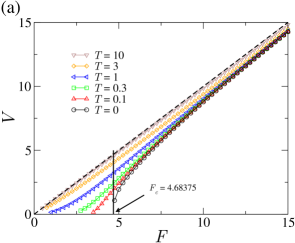
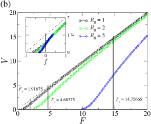
Figure 1: (Color online) (a) Velocity-force characteristics for a single disorder realization of intensity $R_{0}=2$ and different temperatures. (b) Velocity-force characteristic for temperature $T=0.3$ and different disorder intensities as indicated. The inset shows the scaled data according to $v=V/(mF_{c})$ and $f=(F-F_{c})/F_{c}$, where $F_{c}$ is the sample dependent critical force. Furthermore, this rescaling strongly reduces sample-to-sample fluctuations.

In this section we will present the general features of the velocity-force characteristics, allowing us to define the critical region and the scaled variables that will be used throughout the rest of this work. Figure 1(a) shows typical velocity-force curves at finite temperature, as obtained with the present model for $L=1024$ and $M=5792\approx L^{\zeta_{\mathrm{dep}}}$, with $\zeta_{\mathrm{dep}}=1.25$ duemmer2 ; rosso_hartmann the depinning roughness exponent (see below). Given a fixed force $F$, the velocity is computed in the steady state, which is typically reached within one sweep over the transverse size $M$ (as detailed below, the transverse size $M$ will be varied following a scaling relation with the string length $L$). Then, of the order of five sweeps over $M$ are used to compute the velocity

$$V=\langle\partial_{t}u(z,t)\rangle.$$ (4)

The thermal average is taken by computing $200$ values of the velocity with independent thermal noise realizations within this steady state regime. Different curves correspond to the same single disorder realization with intensity $R_{0}=2$ and increasing temperature. The characteristic critical force is indicated in the key. The lower curve, corresponding to $T=0$, clearly presents the typical abrupt depinning transition: the velocity is strictly zero for $F<F_{c}$, while it increases as $(F-F_{c})^{\beta}$ for $F>F_{c}$, where $\beta<1$ is the velocity exponent. As observed, by increasing the temperature the $T=0$ sharp transition is smeared out. Although at very small temperatures the curves still present the curvature corresponding to $(F-F_{c})^{\beta}$, at higher temperatures there are no clear signatures of the underlying $T=0$ depinning transition. Finally, at very high temperatures, when the thermal energy is larger than the typical pinning energy, the velocity tends to increase linearly with the force, $V=mF$, with the mobility $m=1/\gamma$, corresponding to the dashed line in Fig. 1(a).

In Fig. 1(b) the disorder intensity effects on the velocity-force characteristic can be observed. The critical forces for the corresponding disorder realizations for each intensity are quoted. Since around the depinning transition the velocity strongly depends on the sample critical force value, along the present work we will use scaled variables for velocity and force. The scaled velocity is given by

$$v=\overline{\left(\frac{\langle\partial_{t}u(z,t)\rangle}{mF_{c}}\right)}=\overline{\left(\frac{V}{mF_{c}}\right)},$$ (5)

which defines a systematics to average over disorder realizations. Besides, we use as the control parameter the scaled force

$$f=\frac{F-F_{c}}{F_{c}},$$ (6)

which measures the scaled distance to the critical force for each disorder realization. These definitions of scaled variables are different than the scaled variables used in standard critical phenomena. In our case, we are using the critical force of each disorder realization in order to measure how close the system is to the critical point, instead of using the disorder averaged value $\overline{F_{c}}$. Besides, we also incorporate into the definition of the order parameter $v$ a non-trivial disorder average when using the disorder realization dependent value $F_{c}$.

Although a temperature-dependent critical force can be considered for studying thermal properties at depinning blatter_vortex_review , we are using here the zero-temperature value. From a practical point of view the temperature-dependent critical force can be defined as the inflexion point of the velocity-force curves. In fact, in the temperature range we are studying here this temperature-dependent critical force does not deviate much from the zero-temperature value. Instead of using a temperature-dependent critical force, we adhere here to the idea that the important quantity given by the disorder potential is the zero-temperature critical force and that the small temperature data can be interpreted using this quantity. Besides, the zero-temperature critical force strictly depends only on the disorder configuration and therefore permits the computation of the average velocity using Eq. (5) with disorder and temperature averages independently realized.

The scaled variables, Eqs. (5) and (6), are natural for an overdamped particle driven in a periodic potential $U(x)=R_{0}\cos(x/\lambda)$, $\gamma dx/dt=-dU(x)/dx+F$, where one can readily obtain that $F_{c}=R_{0}/\lambda$ and $\gamma V/F_{c}\approx\sqrt{(F-F_{c})/F_{c}}$ close to $F_{c}$. They also arise in functional renormalization group calculations for center of mass velocity of an elastic manifold, $\tilde{\gamma}V/F_{c}\sim[(F-F_{c})/F_{c}]^{\beta}$ but with $\tilde{\gamma}$ an effective friction coefficient chauve_creep_long . On the other hand, from a practical point of view, it was shown that the scaled variables defined in Eqs. (5) and (6), applied to each particular sample, serve to diminish sample-to-sample fluctuations when studying the depinning transition of a string bustingorry_thermal_rounding_epl ; duemmer2 .

The inset of Fig. 1(b) shows the same data as in the main panel but in scaled form for a single realization. The difference between these curves close to the threshold is due to the fact that the full function $V(F,T)$ depends on the disorder intensity not only through the value of the critical force, but one also needs to consider both extra disorder-dependent temperature scale and friction coefficient. This interesting issue will not be crucial for our present study however (see discussion in Sec. VII below).

IV Temperature dependence of the velocity at the critical force

Here we show the finite temperature response of the elastic string exactly at the critical force and discuss some finite size scaling effects, in particular the crossover to single particle dynamics. Figure 2 presents velocity-temperature curves for different system sizes. All the curves were computed at exactly the sample critical force, using the scaled force variable $f=0$, and then averaged over disorder realizations. The disorder intensity is $R_{0}=0.5$ and the results are qualitatively similar to those reported for $R_{0}=1$ in Ref. bustingorry_thermal_rounding_epl . At very high temperatures, $T\gg R_{0}$, the system enters the fast flow regime and the velocity practically equals the force; therefore the reduced velocity (which incorporates the critical force) tends to unity. At intermediate temperatures, the velocity reduces and the curves tend to display the critical behavior $v\sim T^{\psi}$. This power-law behavior is however interrupted by finite-size effects at smaller temperatures, when the dynamic characteristic length $\xi$ equals the system size $L$.

At very small temperatures a crossover to single particle dynamics duemmer2 ; kolton_universal_aging_at_depinning is observed as shown by the $L=32$ curve. A simple ad-hoc model to rationalize this crossover has been given by Duemmer and Krauth duemmer2 while numerically studying the zero-temperature depinning transition. Within this model, one can write the velocity in the very small temperature regime as

$$v=\frac{M}{\tau_{0}+\tau_{1}(T)},$$ (7)

where $\tau_{1}(T)$ is the temperature-dependent time the interface spends near the critical configuration and $\tau_{0}$ is the rest of the time needed to cover the transverse spatial period $M$ of the computational box. In this simple model, $\tau_{0}$ is approximated to be temperature independent at very low temperatures. Using the temperature dependence of the escape rate for a particle in a random potential colet_marginal_thermal_escape , one can propose that $\tau_{1}=aT^{-1/3}$. In Fig. 2 we show with a dotted line that the very small temperature regime for $L=32$ is well fitted with Eq. (7). For $L=32$ and $M=304\approx 4L^{\zeta_{\mathrm{dep}}}$ we fitted the $T<10^{-3}$ regime using Eq. (7) and we found the fitting parameters $\tau_{0}=779.5$ and $a=3.42$. This is a simplified model allowing to rationalize the crossover to one-particle dynamics and should be further tested.

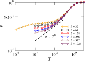
Figure 2: (Color online) Velocity-temperature curves for different systems sizes $L$, as indicated, while keeping $M=4\,L^{\zeta_{\mathrm{dep}}}$, with $\zeta_{\mathrm{dep}}=1.25$ duemmer2 ; rosso_hartmann the depinning roughness exponent. The disorder intensity is $R_{0}=0.5$. All the data were computed at exactly the sample critical force and then averaged over disorder realizations. The dashed line corresponds to the expected power-law behavior. The dotted line describes the crossover to the one-particle regime as discussed in the text.

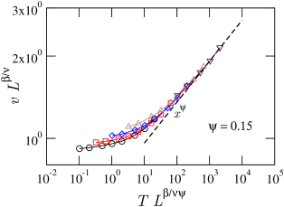
Figure 3: (Color online) Finite size scaling of the velocity-temperature curves for different $L$ values according to Eq. (8). The disorder strength is $R_{0}=0.5$ and the transverse size has been kept at $M=4\,L^{\zeta_{\mathrm{dep}}}$. We show points for $T\leq 0.02$ and $L\geq 64$, since for $L=32$ the single particle regime is present at small temperatures. The dashed line corresponds to the power-law behavior with $\psi=0.15$. We also used the values $\beta=0.33$ duemmer2 and $\nu=1.33$ kolton_short_time_exponents .

The finite size effects displayed by the velocity-temperature curves in Fig. 2 are not easily accounted for by standard finite size scaling arguments. In fact, assuming finite-size scaling as in standard critical phenomena, the velocity should be described by universal functions as in

$$v=L^{-\beta/\nu}g\left(L^{\beta/\nu\psi}\,T\right),$$ (8)

with $g(x)\sim 1$ for $x\ll 1$ and $g(x)\sim x^{\psi}$ for $x\gg 1$. As mentioned in Ref. bustingorry_thermal_rounding_epl strong corrections-to-scaling effects are present in these results. In order to show that, Fig. 3 presents an attempt to use the standard finite size scaling correction scaling, Eq. (8), with the bare data in Fig. 2. One can observe strong finite size corrections and this can also be observed with other values of $R_{0}$. In addition, the collapse of the data does not improve significantly when using other values of the scaling exponents. Despite these strong finite-size effects exhibited by the velocity at critical force, the power-law regime characterized by the thermal rounding exponent $\psi=0.15$ does not suffer from strong finite size effects, as shown in the following sections.

V Structure factor analysis

In this section we turn to the complementary geometrical analysis of the structure factor, which contains information on the geometry of the string at different length scales. The results presented in this section complements those reported in Refs. bustingorry_thermal_rounding_epl ; bustingorry_periodic by including different disorder strengths.

From the numerical simulations, the steady state structure factor is defined as

$$S_{q}=\frac{1}{L}\overline{\left\langle\left|\sum_{j=0}^{L-1}u_{j}\,e^{iqj}\right|^{2}\right\rangle},$$ (9)

where $q=2\pi n/L$, with $n=1,...,L-1$. One can show using dimensional analysis that when the width $w$ of a self-affine interface of size $L$ is described through a roughness exponent $\zeta$, i.e. $w\sim L^{\zeta}$, then the structure factor behaves as $S_{q}\sim q^{-(1+2\zeta)}$ in $1+1$ dimensions.

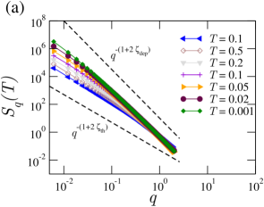
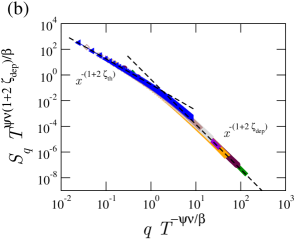
Figure 4: (Color online) (Color online) Structure factor and its scaling function for $R_{0}=0.5$. The curves in (a) correspond to the critical force and different temperatures. The size of the sample is given by $L=1024$ and $M=4L^{\zeta_{\mathrm{dep}}}$. (b) Scaled curves showing the crossover between the depinning regime at small length scales ($x=qT^{-\psi\nu/\beta}\gg 1$) and the thermal regime at large length scales ($x=qT^{-\psi\nu/\beta}\ll 1$). Together with $\psi=0.15$, the values $\beta=0.33$ duemmer2 , $\nu=1.33$ kolton_short_time_exponents and $\zeta_{\mathrm{dep}}=1.25$ duemmer2 ; rosso_hartmann were also used.

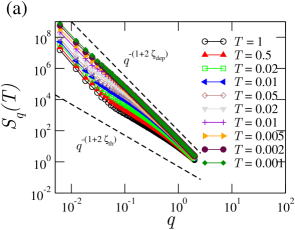
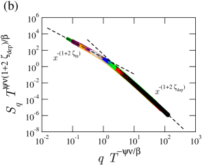
Figure 5: Structure factor and its scaling function for $R_{0}=5$. The curves in (a) correspond to the critical force and different temperatures. The size of the sample is given by $L=1024$ and $M=L^{\zeta_{\mathrm{dep}}}$. (b) Scaled curves showing the crossover between the depinning regime at small length scales ($x=qT^{-\psi\nu/\beta}\gg 1$) and the thermal regime at large length scales ($x=qT^{-\psi\nu/\beta}\ll 1$). The very large length scale random-periodic fast-flow regime has been discarded (see the text). Together with $\psi=0.15$, the values $\beta=0.33$ duemmer2 , $\nu=1.33$ kolton_short_time_exponents and $\zeta_{\mathrm{dep}}=1.25$ duemmer2 ; rosso_hartmann were also used.

At small length scales, $q\gg 1/\xi$, the structure factor shows the typical roughness regime associated to depinning, i.e. $S_{q}\sim q^{-(1+2\zeta_{\mathrm{dep}})}$, while at large length scales, $q\ll 1/\xi$, fluctuations are dictated by effective thermal fluctuations induced by the disorder, i.e. $S_{q}\sim q^{-(1+2\zeta_{\mathrm{th}})}$. The thermal and depinning roughness exponents are, respectively, $\zeta_{\mathrm{th}}=1/2$ and $\zeta_{\mathrm{dep}}=1.25$ rosso_hartmann ; duemmer2 . In the critical region the depinning correlation length is given by the velocity as $\xi\sim v^{-\nu/\beta}$. Thus, the depinning correlation length depends on the temperature only through the velocity and in the thermal rounding regime $\xi\sim T^{-\psi\nu/\beta}$ bustingorry_thermal_rounding_epl . With this information one can write for the structure factor that

$$S_{q}=T^{-\psi\nu(1+2\zeta_{\mathrm{dep}})/\beta}s\left(qT^{-\psi\nu/\beta}\right),$$ (10)

where the scaling function $s(x)\sim x^{-(1+2\zeta_{\mathrm{th}})}$ for $x\ll 1$ and $s(x)\sim x^{-(1+2\zeta_{\mathrm{dep}})}$ for $x\gg 1$. In Ref. bustingorry_thermal_rounding_epl we showed that the structure factor scales with the previous form using $L=1024$ and $M=L^{\zeta_{\mathrm{dep}}}$ for the disorder intensity $R_{0}=1$. Here, we show in Fig. 4(a) the temperature dependence of the structure factor corresponding to $R_{0}=0.5$, $L=1024$ and $M=4L^{\zeta_{\mathrm{dep}}}$. For these parameters the presented data do not show transverse finite size effects bustingorry_periodic . Figure 4(b) shows the scaling of the structure factor according to Eq. (10) and using $\psi=0.15$, which shows a very satisfactory data collapse.

In order to reach the steady-state for the same temperatures of Fig. 4(a) but larger disorder intensities it is necessary to equilibrate the system for longer times. Since this equilibration time scales with the transverse system size we can reduce the simulation time by using $M=L^{\zeta_{\mathrm{dep}}}$ for $R_{0}=5$. The resulting data, shown in Fig. 5(a), presents the small length scale depinning regime and the large scale effective thermal regime described above, but also clearly show a larger length scale regime where finite transverse size effects are present. In this regime the roughness exponent is the one corresponding to a random-periodic system in the fast-flow regime, $\zeta_{\mathrm{per}}=3/2$ bustingorry_periodic . Hence, we can detect and discard the data corresponding to this random-periodic regime in order to get a curve that can be scaled again using Eq. (10) and the known random-manifold exponents, as shown in Fig. 5(b), getting again a very satisfactory collapse.

Therefore, we have presented here data of the structure factor for different disorder intensities which shows that the quoted thermal rounding exponent is disorder independent. Furthermore, we have shown how the thermal rounding exponent gives the temperature dependence of the depinning correlation length, $\xi\sim T^{-\psi\nu/\beta}$, from a steady-state geometry analysis.

VI Short-time dynamics analysis

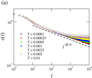
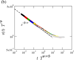
Figure 6: (Color online) (a) Short time evolution of the velocity at the critical force and for different temperatures, from $T=0.0001$ (lower curve) to $T=0.01$ (upper curve), as indicated in the key. Data correspond to $R_{0}=1$, $L=1024$ and $M=L^{\zeta_{\mathrm{dep}}}$.(b) Short time scaling of the velocity for $t>20$. The behavior $x^{-\beta/z\nu}$ for $x=tT^{\psi z\nu/\beta}\ll 1$ is indicated with a dashed line. Together with $\psi=0.15$, the values $\beta=0.33$ duemmer2 , $\nu=1.33$ kolton_short_time_exponents and $z=3/2$ kolton_short_time_exponents were also used.

One possible way to get rid of finite size effects is to analyze the short time dynamics. Starting from a given non-steady initial condition at fixed force $F$ and temperature $T$, the velocity begins to evolve with time until it reaches the steady-state value corresponding to the values of $F$ and $T$. This transient dynamics is controlled, at short times, by a single growing correlation length, $\xi(t)$, which at longer times saturates to the steady-state correlation length above threshold, $\xi\sim v^{-\nu/\beta}$. Since the transient correlation length grows as $\xi(t)\sim t^{1/z}$, with $z\approx 3/2$ kolton_short_time_exponents the depinning dynamical exponent, scaling arguments show that the velocity decreases with time as $v(t)\sim\xi(t)^{-\beta/\nu}\sim t^{-\beta/z\nu}$ kolton_short_time_exponents before saturating to the steady-state value above threshold, given by $v(t\to\infty)\sim f^{\beta}$ at $T=0$ or by $v(t\to\infty)\sim T^{\psi}$ at $f=0$.

Figure 6(a) shows the time evolution of the velocity exactly at the critical force and for different temperature values as indicated. The dashed line corresponds to the expected short-time critical behavior $v(t)\sim t^{-\beta/z\nu}$. Discarding the very short time regime, $t\leq 20$, which contains information about the microscopic non-universal dynamics kolton_short_time_exponents , the curves in Fig. 6(a) can be recast into a universal form using the scaling function

$$v(t)=T^{\psi}h\left(tT^{\psi z\nu/\beta}\right),$$ (11)

with $h(x)\sim x^{-\beta/z\nu}$ for $x\ll 1$ and $h(x)\sim 1$ for $x\gg 1$. The data collapse shown in Fig. 6(b) uses the previously known depinning exponents $\beta=0.33$ duemmer2 , $\nu=1.33$ kolton_short_time_exponents , $z=3/2$ kolton_short_time_exponents , together with the thermal rounding exponent $\psi=0.15$. Since the data collapse is good with no need of adjustable parameters we can conclude that the value of the thermal rounding exponent obtained in Ref. bustingorry_thermal_rounding_epl is consistent and does not suffer from strong finite-size effects.

VII Velocity scaling function around depinning

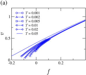
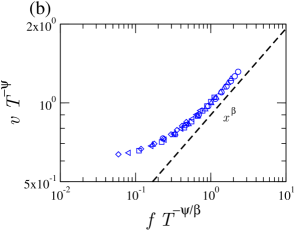
Figure 7: (Color online) (a) Velocity-force characteristics at finite temperatures for $R_{0}=1$. Data shown with points (lines) are inside (outside) the thermal rounding region (see the text). (b) Scaling of the data for $f>0$ and in the thermal rounding region using the scaling form given in Eq. (12). The dashed line indicates the asymptotic expected form $x^{\beta}$ for $x=fT^{-\psi/\beta}\gg 1$. Here, the value $\beta=0.33$ duemmer2 was used together with $\psi=0.15$.

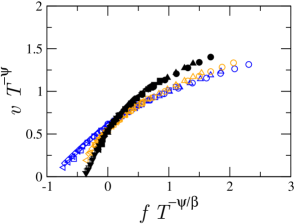
Figure 8: (Color online) Scaling of velocity-force curves for different temperatures and close to the thermal rounding regime. Different disorder intensities are shown: $R_{0}=1$ (blue), $R_{0}=2$ (orange) and $R_{0}=5$ (black). Symbols represent different temperatures as in Fig. 7(a). Here, the value $\beta=0.33$ duemmer2 was used together with $\psi=0.15$.

In this section we turn to the analysis of the universal behavior of the force and temperature dependent velocity function, $v(f,T)$. Focusing on testing the robustness of the thermal rounding exponent $\psi$, parameter values around the critical point given by $f=0$ and $T=0$ are tested. If there were not strong finite size effects, in the vicinity of the critical region the velocity should scale as

$$vT^{-\psi}\sim H\left(fT^{-\psi/\beta}\right),$$ (12)

with $H(x)\sim x^{\beta}$ for $x\gg 1$. Figure 7(a) shows velocity-force curves for different temperatures and for $R_{0}=1$. The numerical data is split into two sets: on the one hand data points correspond to given parameters which are “inside” the thermal rounding region, and on the other hand continuous lines represent data “outside” the thermal rounding region. The data are outside the critical region either because temperature is too high, $T>0.02$ in the present case, or because the force is far away from the critical value, $|f|\gg 1$ ($f\gg 1$ and $f\ll-1$ corresponding to the fast-flow and creep regimes, respectively). In addition, to avoid finite-size effects, data points are also considered “outside” the critical thermal rounding region if they correspond to velocities smaller than the crossover at $v\sim v_{min}$ to single-particle behavior for each size $L$. Since in the critical region $\xi\sim v(f,T)^{-\nu/\beta}$, as shown from the structure factor analysis, we roughly have $v_{min}\sim L^{-\beta/\nu}$. According to such criteria, the selected data is finally presented in the scaled form Eq. (12) in Fig. 7(b) for $f>0$. The dashed line indicates the expected asymptotic $x^{\beta}$ form, corresponding to the scaling function $H$ around the critical region. The collapse into a single curve for different $T$ and $f$ confirms numerically that the data set used is inside the critical scaling region.

The scaling function $H$ is not yet universal as it also depends on the disorder intensity. Figure 7 shows the critical region and the form of $H$ for $R_{0}=1$. In Fig. 8 we show the velocity scaling function $H$ for different disorder intensities, $R_{0}=1,2$ and $5$, for the full force range within the thermal rounding region. In Fig. 9 the same data is presented in a double logarithmic scale. As can be observed all curves display the asymptotic power-law form $H\sim x^{\beta}$ for $f\gg T^{\psi/\beta}$, but with different prefactors for each disorder intensity.

At this point, in order to properly include the disorder intensity on the scaling velocity function and obtain the universal function, a disorder-dependent temperature scale $T_{c}$ is needed. Again, for the simple example of the depinning of a particle in a periodic potential $U(x)=R_{0}\cos(x/\lambda)$, $\gamma dx/dt=-dU(x)/dx+F+\eta(t)$, with $\eta(t)$ a Langevin noise at temperature $T$, it is easy to see, from pure dimensional analysis, that $T_{c}\sim R_{0}$, and therefore $\gamma V/F_{c}=h[(F-F_{c})/F_{c},T/R_{0}]$, where $F_{c}=R_{0}/\lambda$. Such naive approach does not work for the elastic string, as the characteristic energy scale is not simply $R_{0}$ as for the particle, but it arises from the interplay of disorder and elasticity. Although it is not obvious that it should work at depinning, one is tempted to use the scaled temperature $\tau=T/T_{c}$, where $T_{c}=U_{c}/k_{B}$ gives the characteristic energy scale in the creep regime at small forces ioffe_creep ; nattermann_creep . This energy scale is however not universal and depends on microscopic details of the disorder  ioffe_creep ; nattermann_creep ; nattermann_hysteresis_domainwall . The assessment of the full dependence of $U_{c}$ on microscopic parameters is thus not straightforward and from a pragmatic point of view one could directly fit it from the creep law. As shown with numerical simulations within the creep regime, at larger temperatures than the one used here, $U_{c}$ can be fitted from the creep law, but it dependence on $R_{0}$ is not trivial kolton_creep2 . We do not have access to $T_{c}$ with the present numerical results, which focused in the force region around the critical depinning threshold.

Therefore, we can not incorporate at this stage the influence of the disorder intensity in the velocity function. In spite of this, the data displayed in Fig. 8 clearly show that the velocity can be represented in a scaled form, with identical critical exponents, for different disorder intensities. More importantly, these data supports the disorder independent value $\psi=0.15$ tested here.

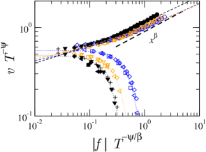
Figure 9: (Color online) Same data as in Fig. 8 but in double-logarithmic representation. The upper and lower curves correspond to $f>0$ and $f<0$, respectively. We also show fitting curves using $a_{1}+a_{2}x^{\beta}$ and $b_{1}\exp[-b_{2}|x|^{\beta/\psi}]$, as suggested by the scaling functions Eqs. (15) and (16).

Finally, it is worth relating our results with the universal scaling function proposed by Nattermann, Pokrovsky and Vinokur nattermann_hysteresis_domainwall using a phenomenological interpolating form for the full force and temperature dependence of the velocity of a domain wall in a random medium. This form includes the thermal rounding regime around $F_{c}$ and the $F\ll F_{c}$ creep regime, thus depending also on the universal creep exponent $\mu=1/4$ (for a one dimensional elastic interface). The proposed functional form in Ref. nattermann_hysteresis_domainwall is different below and above the critical force and can be written as

$$V=mF\frac{\exp\left[-\frac{T_{c}}{T}\left(1-\frac{F}{F_{c}}\right)^{\beta/\psi}\left(\frac{F_{c}}{F}\right)^{\mu}\right]}{1+\left[\frac{T_{c}}{T}\left(\frac{F_{c}}{F}\right)^{\mu}\right]^{\psi}},$$ (13)

for $F<F_{c}$ and

$$V=\frac{mF}{1+\left[\frac{T_{c}}{T}\left(\frac{F_{c}}{F}\right)^{\mu}\right]^{\psi}}+mF\left(1-\frac{F_{c}}{F}\right)^{\beta},$$ (14)

for $F>F_{c}$. It can be shown that close to the depinning region, i.e. above the creep regime, where $f=(F-F_{c})/F_{c}\ll 1$ and $\tau=T/T_{c}\ll 1$ this phenomenological form can be reduced to the scaling form Eq. (12), with $H(x)=H^{-}(x)$ for $f<0$ and $H(x)=H^{+}(x)$ for $f>0$. The corresponding limit functions are

$$H^{-}\left(f\tau^{-\psi/\beta}\right)=e^{-(-f\tau^{-\psi/\beta})^{\beta/\psi}},$$ (15)

$$H^{+}\left(f\tau^{-\psi/\beta}\right)=1+(f\tau^{-\psi/\beta})^{\beta}.$$ (16)

Since we do not have the temperature scale $T_{c}$ from the creep law, we have directly fitted the data for the velocity scaling function to the universal forms suggested by Eqs. (15) and (16). The $f<0$ and $f>0$ ranges have been fitted separately using $a_{1}+a_{2}x^{\beta}$ and $b_{1}\exp[-b_{2}|x|^{\beta/\psi}]$, respectively, obtaining four fitting parameters for each disorder intensity. The results are shown in Fig. 9. In all cases the fit is better in the $f<0$ region. Furthermore, one can observe that the obtained curves interpolate badly around $f=0$. In fact, enforcing $a_{1}=b_{1}$ makes the fitting considerably worse. We therefore conclude that the data can not be satisfactorily fitted using this phenomenological form, particularly above threshold, hence evidently pointing to the need of a more accurate description of the thermal rounding of the depinning transition.

The phenomenological functional forms, Eqs. (13) and  (14), give a potentially important tool which allows to directly fit experimental data. This was directly used in Ref. metaxas_thesis , where the velocity-force characteristic below threshold for ultrathin ferromagnetic layers was fitted using Eq. (13). By fitting just one experimental curve below threshold, the value $\psi=0.15\pm 0.10$ was obtained for the thermal rounding exponent. Since several fitting parameters were used and due to the large error bar, this value can only be compared with our numerical value with extreme caution. Anyway, the experimental value is consistent with our numerical simulations.

VIII Summary

We have presented extensive numerical simulations to test the validity of the thermal rounding exponent of the depinning transition. We analyzed the direct scaling of the steady-state velocity-force characteristics, the steady-state structure factor and the short-time transient dynamics. The existence of a critical (power law) thermal rounding of the depinning transition is consistent with all our results, together with the existence of a unique divergent length scale, dependent on temperature and/or distance to the critical pinning force, but ultimately controlled by the velocity as in the zero temperature depinning transition. The results are all consistent with a value of the thermal rounding exponent of $\psi=0.15$ in agreement with our previously reported value bustingorry_thermal_rounding_epl . This exponent describes the power-law vanishing of the velocity with temperature exactly at the critical depinning force, $V\sim T^{\psi}$, for the universality class of one dimensional elastic interfaces with short-range elasticity and short-range correlations in the disorder.

Although the value of the thermal rounding exponent have been previously obtained with larger system sizes, where finite size corrections are still observable, we have shown here that this value is also consistent with short-time dynamics results which do not suffer from severe finite size effects. Besides, $\psi=0.15$ also describes the scaling properties of the structure factor for various disorder strength values, connecting this value with a geometrical roughness crossover in the interface. Finally, we have shown that it is consistent with a scaling function describing the velocity-force characteristics as a function of temperature and force. Experimental confirmation of our results, directly targeting the thermal rounding regime and allowing to test the value of the thermal rounding exponent, would be welcome.

- (1) S. Lemerle, J. Ferré, C. Chappert, V. Mathet, T. Giamarchi, and P. Le Doussal, Phys. Rev. Lett. 80, 849 (1998)
- (2) M. Bauer, A. Mougin, J. P. Jamet, V. Repain, J. Ferré, R. L. Stamps, H. Bernas, and C. Chappert, Phys. Rev. Lett. 94, 207211 (2005)
- (3) M. Yamanouchi, D. Chiba, F. Matsukura, T. Dietl, and H. Ohno, Phys. Rev. Lett. 96, 096601 (2006)
- (4) P. J. Metaxas, J. P. Jamet, A. Mougin, M. Cormier, J. Ferré, V. Baltz, B. Rodmacq, B. Dieny, and R. L. Stamps, Phys. Rev. Lett. 99, 217208 (2007)
- (5) P. Paruch, T. Giamarchi, and J. M. Triscone, Phys. Rev. Lett. 94, 197601 (2005)
- (6) P. Paruch and J. M. Triscone, Appl. Phys. Lett. 88, 162907 (2006)
- (7) S. Moulinet, A. Rosso, W. Krauth, and E. Rolley, Phys. Rev. E 69, 035103(R) (2004)
- (8) E. Bouchaud, J. P. Bouchaud, D. S. Fisher, S. Ramanathan, and J. R. Rice, J. Mech. Phys. Solids 50, 1703 (2002)
- (9) M. Alava, P. K. V. V. Nukalaz, and S. Zapperi, Adv. Phys. 55, 349 (2006)
- (10) G. Blatter, M. V. Feigel’man, V. B. Geshkenbein, A. I. Larkin, and V. M. Vinokur, Rev. Mod. Phys. 66, 1125 (1994)
- (11) T. Giamarchi and S. Bhattacharya, in High Magnetic Fields: Applications in Condensed Matter Physics and Spectroscopy, edited by C. Berthier et al. (Springer-Verlag, Berlin, 2002) p. 314, cond-mat/0111052
- (12) X. Du, G. Li, E. Y. Andrei, M. Greenblatt, and P. Shuk, Nature Physics 3, 111 (2007)
- (13) T. Nattermann and S. Brazovskii, Adv. Phys. 53, 177 (2004)
- (14) T. Giamarchi, “Quantum phenomena in mesoscopic systems,” in Quantum phenomena in mesoscopic systems (IOS Press, Bologna, 2004) Chap. Electronic Glasses, Italian Physical Society ed., arXiv:cond-mat/0403531
- (15) D. S. Fisher, Phys. Rev. B 31, 1396 (1985)
- (16) A. B. Kolton, A. Rosso, T. Giamarchi, and W. Krauth, Phys. Rev. Lett. 97, 057001 (2006)
- (17) A. B. Kolton, A. Rosso, T. Giamarchi, and W. Krauth, Phys. Rev. B 79, 184207 (2009)
- (18) L. B. Ioffe and V. M. Vinokur, J. Phys. C 20, 6149 (1987)
- (19) T. Nattermann, Europhys. Lett. 4, 1241 (1987)
- (20) M. V. Feigel’man, V. B. Geshkenbein, A. I. Larkin, and V. M. Vinokur, Phys. Rev. Lett. 63, 2303 (1989)
- (21) T. Nattermann, Phys. Rev. Lett. 64, 2454 (1990)
- (22) P. Chauve, T. Giamarchi, and P. Le Doussal, Europhys. Lett. 44, 110 (1998)
- (23) P. Chauve, T. Giamarchi, and P. Le Doussal, Phys. Rev. B 62, 6241 (2000)
- (24) A. A. Middleton, Phys. Rev. B 45, 9465 (1992)
- (25) L. W. Chen and M. C. Marchetti, Phys. Rev. B 51, 6296 (1995)
- (26) U. Nowak and K. D. Usadel, Europhys. Lett. 44, 634 (1998)
- (27) L. Roters, A. Hucht, S. Lübeck, U. Nowak, and K. D. Usadel, Phys. Rev. E 60, 5202 (1999)
- (28) D. Vandembroucq, R. Skoe, and S. Roux, Phys. Rev. E 70, 051101 (2004)
- (29) M. B. Luo and X. Hu, Phys. Rev. Lett. 98, 267002 (2007)
- (30) S. Bustingorry, A. B. Kolton, and T. Giamarchi, Europhys. Lett. 81, 26005 (2008)
- (31) P. Le Doussal, K. J. Wiese, and P. Chauve, Phys. Rev. B 66, 174201 (2002)
- (32) V. Lecomte, S. E. Barnes, J.-P. Eckmann, and T. Giamarchi, Phys. Rev. B 80, 054413 (2009)
- (33) P. J. Metaxas, Domain wall dynamics in ultrathin ferromagnetic film structures: disorder, coupling and periodic pinning, Ph.D. thesis, Université Paris-Sud–University of Western Australia (2009)
- (34) P. J. Metaxas, R. L. Stamps, J.-P. Jamet, J. Ferré, V. Baltz, B. Rodmacq, and P. Politi, Phys. Rev. Lett. 104, 237206 (2010)
- (35) A. Rosso and W. Krauth, Phys. Rev. E 65, 025101R (2002)
- (36) A. B. Kolton, A. Rosso, and T. Giamarchi, Phys. Rev. Lett. 94, 047002 (2005)
- (37) O. Duemmer and W. Krauth, Phys. Rev. E 71, 061601 (2005)
- (38) A. Rosso, A. K. Hartmann, and W. Krauth, Phys. Rev. E 67, 021602 (2003)
- (39) A. B. Kolton, G. Schehr, and P. L. Doussal, Phys. Rev. Lett. 103, 160602 (2009)
- (40) P. Colet, M. San Miguel, J. Casademunt, and J. M. Sancho, Phys. Rev. A 39, 149 (Jan 1989)
- (41) A. B. Kolton, A. Rosso, E. V. Albano, and T. Giamarchi, Phys. Rev. B 74, 140201 (2006)
- (42) S. Bustingorry, A. B. Kolton, and T. Giamarchi, Phys. Rev. B 82, 094202 (2010)
- (43) T. Nattermann, V. Pokrovsky, and V. M. Vinokur, Phys. Rev. Lett. 87, 197005 (2001)
- (44)