GPGPU for orbital function evaluation with a new updating scheme

Abstract

We have accelerated an ab-initio QMC electronic structure calculation using General Purpose computing on Graphical Processing Units (GPGPU). The part of the code causing the bottleneck for extended systems is replaced by CUDA-GPGPU subroutine kernels which build up spline basis set expansions of electronic orbital functions at each Monte Carlo step. We have achieved a speedup of a factor of 30 for the bottleneck for a simulation of solid TiO₂ with 1,536 electrons. To improve the performance with GPGPU we propose a new updating scheme for Monte Carlo sampling, quasi-simultaneous updating, which is intermediate between configuration-by-configuration updating and the widely-used particle-by-particle updating. The error in the energy due to by the single precision treatment and the new updating scheme is found to be within the required accuracy of $\sim 10^{-3}$ hartree per primitive cell.

I Introduction

General Purpose computing on Graphical Processing Units (GPGPU) GPU03 ; GPGPU has attracted recent interest in HPC (High Performance Computing) for accelerating calculations at a reasonable cost. Environments for developing GPGPU, such as CUDA (Compute Unified Device Architecture) CUDA ; CUDA2 , have also contributed to the recent trend for using GPGPU for scientific applications with much increased portability GPGPU . Electronic structure calculations MAR04 form one of the largest fields within HPC and there have been many attempts to accelerate such calculations using GPGPU GPGPU . Electronic structure calculation using quantum Monte Carlo (QMC) methods can provide highly reliable estimates of material properties for a wide range of compounds HAM94 ; FOU01 ; NEE10 . The very high computational demands are not so important because of the inherently high efficiency of massively parallel computational facilities for Monte Carlo computations GIL11 . There have been several attempts to apply GPGPU to ab-initio QMC electronic structure calculations ESL12 ; UEJ11 .

Previously we reported GPGPU acceleration of a QMC calculation for molecular systems, in which we achieved a speedup of more than a factor of 20 UEJ11 . The key idea was to replace only the bottleneck subroutines in the main code by the CUDA kernel running on the GPU. We emphasized that the replacement of the entire simulation code by its GPU version is not practical from the viewpoint of version administration UEJ11 . This becomes more serious for practical program packages with large number of users, as is common in ab-initio electronic structure simulations UEJ11 .

It was challenging to achieve substantial acceleration using such a ‘partial replacement strategy’, and it should give a speedup of at least more than a factor of ten to be advantageous to use multi-core processor technology. In Ref.UEJ11 the main code written in Fortran90 (F90) was partially replaced by the GPU kernel, which were at the object code level. Users could switch back to the original CPU version of the subroutine if the GPU was not available. In the previous study GPGPU was applied to molecular simulations, although solid systems are the most attractive target for GPU-QMC electronic structure simulations FOU01 because of the vast CPU time required and the potential of QMC to achieve more reliable results than frameworks such as density functional theory (DFT).

The bottleneck in the present work differs from that in our previous molecular simulation UEJ11 . In our previous work the bottleneck was the routine for computing the Hartree fields corresponding to the particle configuration MAE07 . In the present work the bottleneck is the routine for evaluating the single particle orbitals at the required particle positions. We have achieved a speedup of more than a factor of 30 with GPGPU compared with the single core performance of the conventional CPU evaluation. This acceleration does not, in principle, harm the MPI (massively parallel interface) parallelization efficiency, which is essentially the same as in our previous work UEJ11 . The conventional MPI parallel evaluation FOU01 can be accelerated further by attaching a GPU to each node. In QMC calculations the electronic orbitals are calculated many times at different electronic positions. It is quite common in ab-initio electronic structure methods, including QMC, that one builds up orbital functions for given electronic positions. Our implementation achieved here would be useful also in self-consistent field (SCF) methods used in density functional theories (DFT) or molecular orbitals (MO) methods.

MPI parallelization has successfully been used in QMC electronic structure calculations HAM94 ; FOU01 ; NEE10 , obtaining $\sim$ 99% parallel efficiency by distributing the huge number of configurations over the processing nodes. On each node the evaluation is usually sequential, though there have been several attempts to exploit further parallelization within the node using, for example, OpenMP NEE10 . The evaluations performed on each node include updating an electronic configuration $\vec{R}^{(\alpha)}=(\vec{r}_{1}^{(\alpha)},\cdots,\vec{r}_{j}^{(\alpha)},\cdots,\vec{r}_{N}^{(\alpha)})$, and sampling with the updated configuration, where $\alpha$ is the index for MC steps. There are two major types of updating scheme, the configuration-by-configuration scheme (simultaneous updating) and the particle-by-particle scheme (PbP, sequential updating). In the former, attempted trial $N$-electron moves are generated to update a configuration, $\vec{R}^{(\alpha)}\to\vec{R}^{(\alpha+1)}$, and then the new configuration is accepted or rejected. In the latter, a trial move of a single electron is attempted and accepted or rejected, $\vec{r}_{j}^{(\alpha)}\to\vec{r}_{j}^{(\alpha+1)}$, and the process is repeated $N$ times. Sequential updating is more efficient than simultaneous updating, and it is widely used in QMC electronic structure calculations NEE10 . For hybrid parallelization, including GPGPU and OpenMP, one seeks further parallelization in the sequential evaluation within an MPI node. The GPGPU performs the accept/reject steps for each particle ‘simultaneously’. The ratio of the probabilities evaluated in the Metropolis accept/reject algorithm HAM94 differs both from those for simultaneous and sequential updating. In this sense our updating scheme can be viewed as ‘quasi-simultaneous updating’ (Q.S.). This scheme is designed to obtain GPGPU acceleration by improving the sequential memory access (so called ‘coalescing’), and the concealment of memory latencies. We have confirmed that our new updating scheme does not change the results within the required statistical accuracy, namely the chemical accuracy.

The paper is organized as follows. In §II we briefly summarize the VMC method (Variational Monte Carlo method). The evaluation of the orbitals represented in a spline basis set is the bottleneck in the computation, as described in this section. The benchmark systems used in the performance evaluation are also introduced. §III is devoted to a description of the GPU architecture. The structure of processors and memories in the GPU used in the present work is briefly explained. Other features, such as how we assign the number of threads and blocks for parallel processing, are discussed in §IV, in connection with the design and implementation of the quasi-updating scheme. The quasi-updating scheme is also introduced in this section. Several other possible implementations with different updating schemes or thread/block assignments are introduced here and their performances are compared. The results are summarized in §V, including comparisons of the energies, operation costs and data transfers, and the dependence of the performance on system size. In §VI we discuss the results, comparing with the ideal performance in terms of operations and memory access. We also discuss the possibility of using high-speed memory devices in the GPU and the relation to linear algebra packages.

II QMC electronic structure calculation

II.1 VMC

In ab-initio calculations the system is specified by a hermitian operator $\hat{H}$ called the Hamiltonian PAR94 . The operator includes information about the positions and charges of the ions, the number of electrons, and the form of the potential functions in the system. The fundamental equation at the electronic level is the many-body Schrödinger equation, which takes the form of a partial differential equation with $\hat{H}$ acting on a multivariate function $\Psi\left(\vec{r}_{1},\cdots,\vec{r}_{N}\right)$, known as the many-body wave function, where $N$ denotes the number of electrons. The energy of the system, $E$, is the eigenvalue of the partial differential equation. The equation has the variational functional HAM94

$$E = \frac{\int\Psi^{*}\hat{H}\Psi\,d{\vec{r}_{1}}\cdots d{\vec{r}_{N}}}{\int\Psi^{*}\Psi\,d{\vec{r}_{1}}\cdots d{\vec{r}_{N}}}$$ (1)

$$= \frac{\int|\Psi|^{2}\cdot\Psi^{-1}\hat{H}\Psi\,d{\vec{r}_{1}}\cdots d{\vec{r}_{N}}}{\int|\Psi|^{2}\,d{\vec{r}_{1}}\cdots d{\vec{r}_{N}}},$$

which is minimized when the above integral is evaluated with $\Psi$ being an exact solution of the eigen equation. For a trial $\Psi$ the functional can be evaluated as an average of the local energy, $E_{L}\left(\vec{r}_{1},\cdots,\vec{r}_{N}\right)=\Psi^{-1}\hat{H}\Psi$ over the probability density distribution

$$p(\vec{r}_{1},\cdots,\vec{r}_{N})=|\Psi|^{2}/\int|\Psi|^{2}\,d{\vec{r}_{1}}\cdots d{\vec{r}_{N}}\ .$$ (2)

In VMC the energy is evaluated by Monte Carlo integration using the Metropolis algorithm to generate configurations $\left\{\vec{R}^{(\alpha)}\right\}_{\alpha=1}^{M}$ distributed according to the probability distribution $p(\vec{r}_{1},\cdots,\vec{r}_{N})=p(\vec{R})$, where $\vec{R}$ denotes a configuration $(\vec{r}_{1},\cdots,\vec{r}_{N})$, as

$$E=\frac{1}{M}\sum_{\alpha=1}^{M}{E_{L}\left(\vec{R}^{(\alpha)}\right)}\ ,$$ (3)

with $M$ being typically of the order of millions. The trial function $\Psi$ is improved by an optimization procedure so that the integral of Eq. (1) can be minimized numerically Optimization1 ; Optimization2 . Since each $E_{L}\left(\vec{R}^{(\alpha)}\right)$ is evaluated independently, the summation over $\alpha$ can be divided into sub-summations distributed over the processors by MPI with high efficiency FOU01 . In this work GPGPU is used to accelerate the evaluation of each $E_{L}\left(\vec{R}^{(\alpha)}\right)$, rather than parallelization over the suffix $\alpha$. We used the ‘CASINO’ program package NEE10 for the VMC calculations.

There are several possible forms of trial $\Psi$, and we chose to use the common Slater-Jastrow type wave function FOU01 ; HAM94 ,

$$\Psi_{\rm SJ}\left({\vec{R}}\right)=e^{J\left({\vec{R}}\right)}\cdot\Psi_{\rm D}\left({\vec{R}}\right)\ ,$$ (4)

where $e^{J\left({\vec{R}}\right)}$ is known as the Jastrow factor JAS55 ; Neil_jastrow . $\Psi_{\rm D}$ is a Slater determinant ASH76

$$\Psi_{\rm D}\left({\vec{r}_{1},\cdots,\vec{r}_{N}}\right)=\left|{\begin{array}[]{*{20}c}{\psi_{1}\left({\vec{r}_{1}}\right)}&\cdots&{\psi_{N}\left({\vec{r}_{1}}\right)}\\ \vdots&\ddots&\vdots\\ {\psi_{1}\left({\vec{r}_{N}}\right)}&\cdots&{\psi_{N}\left({\vec{r}_{N}}\right)}\\ \end{array}}\right|\ ,$$ (5)

which is an anti-symmetrized product of one-particle orbital functions, $\left\{\psi_{l}\left({\vec{r}}\right)\right\}_{l=1}^{L}$. The number of independent orbitals, $L$, can be reduced by using the symmetries of the system. The bottleneck of the whole simulation has been found to be the construction of the $\left\{\psi_{l}\left({\vec{r}}\right)\right\}$ NEE10 . In this study the computational power of the GPU is devoted to the bottleneck process, as described in the following subsection.

II.2 Orbital evaluation

In each MPI process the following evaluations are performed sequentially:

1. An attempted move, $\vec{R}^{(\alpha)}\to\vec{R}^{(\alpha+1)}$, is randomly generated,

2. The updated probability $p(\vec{R}^{(\alpha+1)})$ and the ratio $\xi=p(\vec{R}^{(\alpha+1)})/p(\vec{R}^{(\alpha)})$ is evaluated,

3. Based on the ratio $\xi$, the attempted move $\vec{R}^{(\alpha+1)}$ is accepted or rejected,

4. The local energy $E_{L}\left(\vec{R}^{(\alpha+1)}\right)$ is evaluated.

Each configuration is a set of electronic positions (we omit the spin coordinate for simplicity), $\vec{R}^{(\alpha)}=(\vec{r}^{(\alpha)}_{1},\vec{r}^{(\alpha)}_{2},\cdots,\vec{r}^{(\alpha)}_{j},\cdots,\vec{r}^{(\alpha)}_{N})$. Following Eqs. (2), (4), and (5), one can reduce the evaluation of the ratio $\xi=p(\vec{R}^{(\alpha+1)})/p(\vec{R}^{(\alpha)})$ to that of the orbital functions, $\left\{\psi_{l}\left({\vec{r}^{(\alpha+1)}_{j}}\right)\right\}$. In practical QMC calculations for extended systems the orbital functions are expanded in a $B$-spline basis set $\left\{\Theta_{s}\left({\vec{r}}\right)\right\}$ ALF04 ; MAE09 ; NEE10 as

$$\psi_{l}\left({\vec{r}_{j}}\right)=\sum\limits_{s=1}^{4^{3}=64}{a_{ls}\cdot\Theta_{s}\left({\vec{r}_{j}}\right)}\ .$$ (6)

The index $s$ runs over the subset of the spatial sites within the unit cell of the periodic system. The spline basis functions, $\left\{\Theta_{s}\left({\vec{r}}\right)\right\}$, have non-zero values only at sites $s$ within the fourth nearest neighbor of the position $\vec{r}$ along each direction. The total number of terms in the summation (6) is therefore 64 = 4³ (four spatial points along each direction in the three dimensional space), as a subset of the whole lattice within the unit cell amounting to $S=50^{3}\sim 60^{3}$. The lattice is indexed by $\left\{\tilde{s}\right\}_{\tilde{s}=1}^{S}$, as depicted schematically in the two dimensional plane in Fig. 1. The subset $\left\{s\right\}_{s=1}^{4^{3}}\subset\left\{\tilde{s}\right\}_{\tilde{s}=1}^{S=50^{3}\sim 60^{3}}$ is the spatial region where $\left\{\Theta_{s}\left({\vec{r}}\right)\right\}$ has non-zero values, depending on the given $\vec{r}$. Since the indices introduced so far are complicated we summarize them in Table 1.

Table 1: Conventions for indices used in this paper.

	Index	Total Amount	Reference
Configurations	$\alpha$	$M\sim$ millions	Eq. (3)
Orbitals	$l$	$L<N$	Eq. (5)
Electrons	$j$	$N$	§II.B
Blip Grid (subset)	$s$	$4^{3}=64$	Eq. (6)
Blip Grid (whole)	$\tilde{s}$	$S=50^{3}\sim 60^{3}$	Eq. (8)

The value of $\Theta_{s}\left({\vec{r}}\right)$ at a $s$-lattice site, $\vec{R}_{s}=(X_{s},Y_{s},Z_{s})$, is given by the function depending on the distance between $\vec{r}$ and $\vec{R}_{s}$ as,

$$\Theta_{s}\left({\vec{r}}\right)=\varphi\left({\frac{{x-X_{s}}}{b_{x}}}\right)\cdot\varphi\left({\frac{{y-Y_{s}}}{b_{y}}}\right)\cdot\varphi\left({\frac{{z-Z_{s}}}{b_{z}}}\right)\ ,$$ (7)

where $\varphi\left(\zeta\right)$ is a second order polynomial in $\zeta$, and $(b_{x},b_{y},b_{z})$ denote grid spacings for each direction. The coefficients in Eq. (6), $\left\{{{{\tilde{a}}_{l,\tilde{s}}}}\right\}_{\tilde{s}=1}^{{S\sim 250,000}}$, are precomputed and provided as an input file, stored in memory at the beginning of the simulation. For each MC step with a updated particle position $\vec{r}_{j}$, the subset

$$\left\{{\left\{{{a_{l,s\left({{{\vec{r}}_{j}}}\right)}}}\right\}_{s=1}^{64}}\right\}_{j=1}^{N}\subset\left\{{{{\tilde{a}}_{l,\tilde{s}}}}\right\}_{\tilde{s}=1}^{{S}}$$ (8)

is identified and used in the summation (6). Denoting $a_{l,s\left({\vec{r}_{j}}\right)}=a\left[{l,j_{x},j_{y},j_{z}}\right]$ as an array, $s\left({\vec{r}_{j}}\right)=(j_{x},j_{y},j_{z})$ forms a simply connected region in the three dimensional space but it does not allow sequential memory access in one dimensional address space, as it is interrupted with some stride due to the higher dimensions (see Fig. 1). The orbital index $l$, is, however, inherently one dimensional and we exploit this for sequential memory access, which is very important for GPGPU, as discussed in §IV.B.

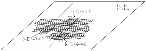
Figure 1: Data structure for the expansion coefficients of the orbital functions in Eq. (6), schematically depicted in two dimensional space. Black lattice points show the nearest site for each given $\vec{r}_{j}$. In the shaded regions the basis functions $\left\{\Theta_{s}\left({\vec{r}_{j}}\right)\right\}$ in Eq. (6) have non-zero values.

We have identified the ‘multiply and add’ operations in Eq. (6), by which the orbital functions, $\left\{\psi_{l}\left({\vec{r}_{j}}\right)\right\}_{l=1}^{L}$, are evaluated as the bottleneck in the present QMC simulation NEE10 . This operation appears at every MC step when the particle position is updated, $\vec{r}_{j}^{(\alpha)}\rightarrow\vec{r}_{j}^{(\alpha+1)}$. The number of operations for a single evaluation is proportional to the number of orbitals, $L$, and hence to $N$. In the present study we treat system sizes up to $L=384$ and $N$=1,536.

II.3 Benchmark systems

To investigate the dependence of the acceleration on system size, we prepared three different benchmark systems, as reported in Table 2. For each system the atomic cores are replaced by pseudopotentials MAR04 in Si-diamond ($N$=216) and cubic TiO₂ ($N$=648 and 1,536). The periodic boundary conditions for $(3\times 3\times 3)$ or $(4\times 4\times 4)$ arrays of unit cells form a simulation cell. More detailed specifications for each system are given in Ref. MAE10 for Si and Ref. MOH12 for TiO₂.

Table 2: Benchmark systems used in the present study. $N$ and $L$ denote the number of electrons and orbitals for each system, respectively. The timing data and the acceleration factors achieved by the best coding are summarized, see §V.A.

System	$N$	$L$	CPU time (ms)	GPU time (ms)	Acceleration factor
Si ($3\times 3\times 3$)	216	56	2.77	0.17	16.58
TiO2 ($3\times 3\times 3$)	648	168	20.21	0.82	24.46
TiO2 ($4\times 4\times 4$)	1,536	384	100.00	3.26	30.67

The bottleneck routine (orbital evaluation) to be replaced by the GPU processing kernel occupies 20$\sim$30% of the entire CPU time for TiO₂ ($N$=1,536), as analyzed by a profiler (Intel VTune Amplifier vtune ). This depends on the choice of the ‘dcorr’ parameter in CASINO NEE10 ; HON10 , which specifies the interval between sampling; in order to reduce the correlation in the sampling, the local energy is evaluated every ‘dcorr’ MC steps (an MC step corresponds to the update of a configuration). The ratio of the CPU time spent in the bottleneck is reduced from 39.5% to 22.0% by increasing ‘dcorr’ from one to ten, as measured for a simulation with 10,000 MC steps. Typically ‘dcorr = 5’ is chosen, for which the reduction becomes 27.5%. The reason for this dependence is that the orbital evaluation is called not only by the configuration updating but also by the local energy evaluation. Increasing ‘dcorr’ means less frequent evaluation of the local energy and hence less frequent calls to the orbital evaluation.

III GPU

General descriptions of the architecture of a GPU can be found in the literature GPGPU ; CUDA ; CUDA2 , and our previous paper UEJ11 also provides such a description. This section provides the minimum amount of information required to understand the present work which was performed with the NVIDIA GeForce GTX 480 architecture.

A GPU has hundreds of processing cores. The key points for the acceleration in the present work can be summarized as follows: (1) Parallelized tasks are distributed over many cores. The large number of processing cores of a GPU allows the whole task to be processed more rapidly than by a CPU. (2) The parallelized tasks are grouped into several sets (called ‘warps’). The GPU processes each warp in order (‘barrel processing’), skipping those still waiting for data load from memory. As there are usually hundreds of warps, barrel processing conceals the memory latency. In our previous work UEJ11 the acceleration was achieved mainly by dividing a huge number of loops into several subsets and distributing them over GPU processor cores. The present work does not follow this strategy, and we do not divide the loop for the summation in Eq. (6). Instead a huge number of independent parallel tasks, $N\times L=1,536\times 384=589,824$, for the orbitals $\left\{\left\{\psi_{l}\left({\vec{r}^{\prime}_{j}}\right)\right\}_{l=1}^{L}\right\}_{j=1}^{N}$ are distributed over the GPU processing cores. Other key points for the present work include, (3) memory latency is much improved when the access occurs with sequential memory address (memory coalescing), and (4) a command set called a ‘Fused Multiply Add (FMA) which performs multiply and add operations within a clock cycle (two operations at once).

III.1 Processors and performance

GTX480 has 480 processor cores, each of which is termed a ‘streaming core’ (SP) for AMD products while ‘cuda core’ is used for NVIDIA products. In the present paper we use the term SP. The specs of the GTX480 are summarized in Table 3. As shown in Fig. 2 every 32 SPs are grouped into a unit called a Streaming Multi-Processor (SM), the total number of which is hence fifteen. Each SP includes 32 bit scalar operators for floating point (FP32) and integer (Int32) data. These two operators can process the data independently within a clock cycle, giving a contribution to the ideal performance with 2 OP/cycle (two operations per clock cycle) for single precision operations. For double precision each 32 bit operator deals with 64 bit floating point (integer) data with two clock cycles, termed FP64 (Int64), giving a 1 OP/cycle contribution on average for double precision operations. There is another kind of operation unit called a ‘Special Function Unit’ (SFU), devoted to evaluating hyper functions including exponential, logarithmic, and trigonometric functions. Each SM includes four SFUs in addition to the 32 SPs. A SFU performs four floating point operations per clock cycle, in parallel with other SM operations, which therefore contributes a further 4 OP/cycle to the ideal performance.

Table 3: Spec of the NVIDIA GTX480 GPU architecture used in the present work.

Compute Capability	2.0
Clock of CUDA cores	1401 MHz
Global Memory	1536 MB
Memory Bandwidth	177.4 GB/s
Number of SM	15
Number of CUDA Cores	480
Constant Memory	64 KB
Shared / L1 Memory	16 or 48 KB per block
Max number of Threads	1024 per block

With a clock frequency of 1.401 GHz, the peak performance of GTX480 is hence evaluated as

$${\rm{1.401GHz}}\times 15{\rm{SM}}\times({\rm{32SP}}\times{\rm{2OP}}+{\rm{4SFU}}\times{\rm{4OP)=1,681[GFlops]}}\ .$$

Note that, unlike the previous GTX275, multiply-and-add operations are not subject to a SFU in the present GTX480. For evaluating Eq. (6) there is hence no place for a SFU to be applied, giving an ideal performance to be compared with our achievement of

$${\rm{1.401GHz}}\times 15{\rm{SM}}\times({\rm{32SP}}\times{\rm{2OP)=1,345[GFlops]\ ,}}$$

by omitting the contribution from SFU. Though the present work concentrates on single precision GPU evaluation, the ideal double precision performance is estimated to be 672 [GFlops], which is half of that for single precision. GeForce GTX480, however, limits it to a quarter of this value, 168 [GFlops], by its driver, for some reason UEJ11 . These estimates are summarized in Table 4, compared with that of the CPU (Intel Core i7 920) used in the present work.

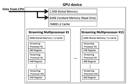
Figure 2: A schematic picture of the structure of the GPU device used in the present work.

Table 4: Estimated ideal performances of GTX480 to be compared with our achievement. The peak performance of the Intel Core i7 CPU is also listed for reference. Note that the ‘ideal’ performance differs from the peak performance of the device (see the text).

	Clock freq.	No. of	Ideal Performance
	(GHz)	cores	(GFlops)
GPU (GTX480) Single precision	1.401	480	1,345
GPU (GTX480) Double precision	1.401	240	672 (limited 168)
CPU (Intel Core i7 920)	2.66	4	42.56

Table 5 summarizes the specification of a computational node used for the experiments. On each node an Intel Core i7 920 processor INT09 and a GPU is mounted on a mother board. Hyper-Threading HTT in the Core i7 processor is turned off, and it is used purely as a four-core CPU. Compute Capability specifies the version of hardware level controlled by CUDA, above ver.1.3, which supports double precision operations. We used the Intel compiler version 12.0.0 for Fortran/C codes using options, ‘-O3’ (optimizations including those for loop structures and memory accesses), ‘-no-prec-div’ and ‘-no-prec-sqrt’ (acceleration of division and square root operations with slightly less precision), ‘-funroll-loops’ (unrolling of loops), ‘-no-fp-port’ (no rounding for float operations), ‘-ip’ (interprocedural optimizations across files), and ‘-complex-limited-range’ (acceleration for complex variables). For CUDA we used the nvcc compiler with options ‘-O3’ and ‘-arch=sm_13’ (enabling double precision operations).

Table 5: Setup of a computational node.

CPU	Intel Core i7 920 2.66 GHz
GPU	NVIDIA GeForce GTX480 $\times$ 1
Motherboard	MSI X58M
Memory	DDR3-10600 2GB $\times$ 6
OS	Linux Fedora 13
Fortran/C Compiler	Intel Fortran/C Composer XE 12.0.0
CUDA	CUDA version 4.0

III.2 Memory architecture

It is essential in GPGPU coding to design efficiently the parallelized tasks (termed ‘threads’) to be grouped into subsets with several different classes. With the variety of memory devices provided in a GPU, see Table 6, each subset has a different ‘distance’ from these devices. The performance of the GPGPU is critically affected by the choice of theses subsets because a good design can effectively reduce the memory latency. In the present study all of the threads are grouped into ‘blocks’. Threads within a block can share memory devices with fewer latencies.

Each block is assigned to a SM by which the threads within the block are processed. The SM processes 32 threads at once, as in vector processing. A bunch of 32 threads is called a ‘warp’. When a warp accesses with sequential memory addresses, the latency is much reduced (called ‘coalescing’). To conceal the memory latency, the scheduler and dispatcher for warps monitor which warps are immediately executable (namely which ones have already completed their memory loads). Then the scheduled warps are processed sequentially by the SM. A schematic picture is shown in Fig. 3.

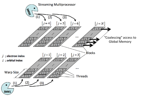
Figure 3: A schematic picture showing the relation between blocks, threads, and streaming multiprocessors (SM).

Table 6 contains only those kinds of memory relevant to this study, and excludes the texture memory CUDA2 . Off-chip memories are located within the GPU board but not on the device chip. They have larger capacities and are accessible directly from CPU hosts but are in general slower. On-chip memories are complementary, namely with higher speed and lower capacity. Data required for GPU processing is transferred from the mother board to off-chip global memory, and is then loaded to on-chip shared memory, as usual.

The capacity of the global memory ranges from 1 GB to 3 GB, depending on the product. As a trade-off against the large capacity it is about 100 times slower than on-chip memories. In GTX480, 768 KB of off-chip L2 cache is available to cover the low speed of the global memory. Another off-chip memory with high speed accessibility is the 64 KB constant memory. Via the constant caches located on every SM the constant memory can be accessed from all the threads with higher speed, although it is limited to read-only. As its name suggests, it is used to store constants referred to by threads. On-chip memories inside each SM include registers, shared memories, and L1 caches. In GTX480 there are 32,768 registers available for each SM. Registers are usually used to store the loop index variables defined within kernel codes, as in the present study. The 64 KB memory device on each SM can be shared by all the threads within a block with high speed access. The 64 KB capacity is divided into 48 KB and 16 KB parts which work as a shared memory and L1 cache, respectively. The user can specify which 48 or 16 KB region corresponds to the shared memory or L1 cache when the kernel code is compiled. The access to the global memory refers first to L1 cache and then L2 and finally to the off-chip global memory device when it fails to load from cache, which are called cache misses.

Data loading from the global memory takes at least 200 cycles, and more usually 400 $\sim$ 600 cycles. To conceal the latency, the GPU administrates all of the warps and monitors whether it is ready to be executed with the completion of data load. With sufficient warps one can ensure that the processors are almost always executing operations without waiting for data loads. To achieve better concealment it is essential to design the code so that it maintains a large number of warps. Since it depends on the specs of each architecture, such as the number of threads per warp, and the maximum possible number of threads per block etc., programming for better performance requires tuning for each GPU product.

	Location	Cache	R/W	Availability	Data maintained
Register	On-chip	-	R/W	within a thread	during a thread
Local memory	Off-chip	L1/L2	R/W	within a thread	during a thread
Shared memory	On-chip	-	R/W	from all threads	during a block
				within a block
Global memory	Off-chip	L1/L2	R/W	from all hosts	during host code
				and threads	maintains
Constant memory	Off-chip	Yes	R	from all hosts	during host code
				and threads	maintains

Table 6: Various kinds of memory in a GPU relevant to this study. R and W stand for readable and writable, respectively.

IV Coding

Only the bottleneck routine for evaluating Eq. (6) is replaced by the CUDA kernel code executed on the GPU. The interface between the main code in F90 and the CUDA kernel is the same as that in our previous study UEJ11 .

IV.1 Quasi-simultaneous updating

To construct appropriate parallelized degrees of freedom, we introduced a new scheme for the MC updating of configurations. Let us denote a configuration at MC step $\alpha$ by $\vec{R}^{(\alpha)}=(\vec{r}_{1}^{(\alpha)},\cdots,\vec{r}_{j}^{(\alpha)},\cdots,\vec{r}_{N}^{(\alpha)})$, and consider the update of a particle position $\vec{r}_{j}^{(\alpha)}\rightarrow\vec{r}^{(\alpha+1)}_{j}$. In configuration-by-configuration updating (simultaneous updating), the accept/reject of the updating is evaluated based on the ratio of the probabilities in Eq. (2),

$$\xi_{\rm sim}=\frac{{p\left({\vec{r}^{(\alpha+1)}_{1},\cdots,\vec{r}^{(\alpha+1)}_{j-1},\vec{r}^{(\alpha+1)}_{j},\vec{r}^{(\alpha+1)}_{j+1},\cdots,\vec{r}^{(\alpha+1)}_{N}}\right)}}{{p\left({\vec{r}_{1}^{(\alpha)},\cdots,\vec{r}_{j}^{(\alpha)},\cdots,\vec{r}_{N}^{(\alpha)}}\right)}}\ ,$$ (9)

while in particle-by-particle (PbP, sequential updating),

$$\xi_{\rm seq}^{\left(j\right)}=\frac{{p\left({\vec{r}^{(\alpha+1)}_{1},\cdots,\vec{r}^{(\alpha+1)}_{j-1},\vec{r}^{(\alpha+1)}_{j},\vec{r}_{j+1}^{(\alpha)},\cdots,\vec{r}_{N}^{(\alpha)}}\right)}}{{p\left({\vec{r}^{(\alpha+1)}_{1},\cdots,\vec{r}^{(\alpha+1)}_{j-1},\vec{r}^{(\alpha)}_{j},\vec{r}_{j+1}^{(\alpha)},\cdots,\vec{r}_{N}^{(\alpha)}}\right)}}\ .$$ (10)

The index $j$ in $\xi_{\rm seq}^{\left(j\right)}$ means that the accept/reject step is made for each particle move, unlike in configuration-by-configuration updating. These two updating schemes give slightly different values for the statistical estimates because of the different paths of the evaluations, but they coincide with each other within the statistical errors. We introduce another updating scheme based on the ratio

$$\xi_{\rm q.sim}^{\left(j\right)}=\frac{{p\left({\vec{r}^{(\alpha)}_{1},\cdots,\vec{r}^{(\alpha)}_{j-1},\vec{r}^{(\alpha+1)}_{j},\vec{r}_{j+1}^{(\alpha)},\cdots,\vec{r}_{N}^{(\alpha)}}\right)}}{{p\left({\vec{r}_{1}^{(\alpha)},\cdots,\vec{r}_{j}^{(\alpha)},\cdots,\vec{r}_{N}^{(\alpha)}}\right)}}\ ,$$ (11)

termed ‘quasi-simultaneous updating’ (Q.S.). In this scheme the accept/reject evaluation for the $j$th particle at step $(\alpha+1)$ is based on the previously fixed $\alpha$ step configuration and on each particle position $j$, which gives $N$ individual parallel tasks.

Evaluating Eq. (11) reduces to computing the orbital functions with updated positions, $\left\{\left\{\psi_{l}\left({\vec{r}^{(\alpha+1)}_{j}}\right)\right\}_{l=1}^{L}\right\}_{j=1}^{N}$, which requires $(N\times L)$ independent evaluations. New trial moves at the $(\alpha+1)$ step

$$(\vec{r}_{1}^{(\alpha)},\cdots,\vec{r}_{j}^{(\alpha)},\cdots,\vec{r}_{N}^{(\alpha)})\rightarrow(\vec{r}_{1}^{(\alpha+1)},\cdots,\vec{r}_{j}^{(\alpha+1)},\cdots,\vec{r}_{N}^{(\alpha+1)})\ ,$$ (12)

are generated on a CPU and sent to a GPU and the orbital functions are evaluated (see Fig. 4). For TiO₂ (4$\times$4$\times$4) this gives $N\times L=1536\times 384=589,824$ parallelized tasks. Note that the parallelized multiplicity $(N\times L)$ scales as $N^{2}$ since the number of orbitals $L\propto N$. The concealment of memory latency is more efficient when the multiplicity increases, and hence we expect better performance for larger systems.

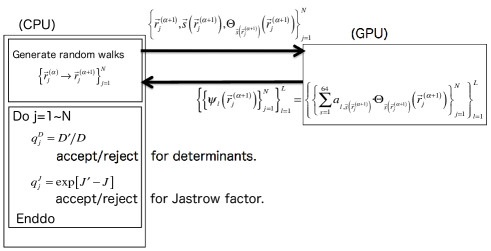
Figure 4: Data transfer between a CPU and GPU in the present implementation. Trial moves for particle positions are generated and sent to a GPU. The GPU computes updated values of the orbitals to send back to the CPU. The accept/reject evaluation based on the orbital values are performed on the CPU.

IV.2 Assigning blocks

Each thread evaluating $\psi_{l}\left({\vec{r}^{(\alpha+1)}_{j}}\right)$ is labelled by $(j,l)$. As mentioned in §II.B, the memory access for the coalescing should take $l$ as the sequential index for the data load of $a_{l,s\left({\vec{r}_{j}}\right)}=a\left[{l,j_{x},j_{y},j_{z}}\right]$, as required for Eq. (6). We therefore assigned the threads sharing the same $j$ with sequentially varying $l=1\sim L$ within a block for the coalescing. The number of orbitals, $L$, cannot therefore exceed the maximum possible number of threads within a block, which is 1,024 for GTX480. The number $L$ can usually be reduced to $L<N$ using the symmetry of the system. It is then a natural choice to assign $L$ within a block rather than $N$, which is always being larger than $L$. For non-magnetic solid systems as in the present work, $L$ is reduced to $\sim N/4$ by the symmetries, giving the limit $N\lesssim$ 4,096 for GTX480. For magnetic systems, $L\sim N/2$, and hence $N\lesssim$ 2,048, and for systems without time-reversal symmetry it becomes 1,024. This limitation is consistent with the maximum simulation size of contemporary QMC electronic structure calculations, which are able to treat at most a few thousand electrons in extended systems MAE10 . Furthermore the limit of 1,024 in GTX480 is expected to double in future architectures , making this issue less important.

When evaluating Eq. (6), all the threads within a block refer to the same $\Theta_{s}\left({\vec{r}_{j}}\right)$ with fixed $j$. Once a warp loads $\left\{\Theta_{s}\left({\vec{r}_{j}}\right)\right\}_{s=1}^{64}$, these data are stored in L1 and L2 cache including their neighboring data. We can then expect effective cache hits for the data load. The operation of each thread, 64 terms multiply and add, easily fits the FMA of the GPU.

IV.3 Other code prepared for comparisons

We prepared several other versions of the code with different updating schemes and thread/block assignments, in order to compare the performance. The original CPU implementation provided by the CASINO distribution NEE10 is the particle-by-particle (PbP) algorithm, with double precision updating, which we refer to as [(0a) CPU/PbP]. Another version, [(1) GPU/PbP], is the GPU version of (0a) but with single precision updating, which is useful for studying deviations between single and double precision computations. In this version the GPU kernel is called with a single fixed $j$ (PbP). Each term, $a_{ls}\cdot\Theta(\vec{r}_{j})$ in the summation of Eq. (6), labelled by $s$, is calculated by each thread, the sum of which is obtained by the reduction operation CUDA2 among all threads. The threads indexed by $s$ are grouped into those sharing the same $l$ and hence the blocks are labelled by the orbital index $l$. Another reference is the version [(2) GPU/Q.S./non-coalescing], which uses quasi-simultaneous (Q.S.) updating, but the same thread/block assignment as the version (1), namely each thread calculates only the product $a_{ls}\cdot\Theta(\vec{r}_{j})$. In this case the blocks are labelled by $(j,l)$. Coalescing does not work in this version. The indices for threads and blocks are summarized in Table 7. Comparing (1) and (2) shows firstly how the performance in speed is improved by the simultaneous data transfers for $j=1\sim N$ in Q.S. compared to the sequential transfers in PbP. Secondly we can see how much the energy deviates due to using Q.S. updating instead of PbP. Our final implementation, described in §IV.B, is termed [(3) GPU/Q.S./coalescing]. The comparison between (1) and (2) is within the single precision treatment. To compare the Q.S. scheme in single and double precision we also prepared [(0b) CPU/Q.S.], which is a double precision version of Q.S.

V Results

V.1 Acceleration performance

Tables 7 and 8 summarize the acceleration factors and computational time taken for the bottleneck kernel part within a MC step. The results are evaluated for systems with $N$ = 216 (Si, $3\times 3\times 3$) and 1,536 (TiO₂, $4\times 4\times 4$). A better performance was obtained using implementation (3) rather than (2) and (1), and with larger system sizes $N$.

Table 7: Comparison of acceleration factors for each implementation evaluated from Table 8. ‘PbP’ and ‘Q.S.’ stand for the particle-by-particle and quasi-simultaneous updating schemes, respectively. The ‘Index’ column shows which indices in Eq. (6) are assigned to threads and blocks in the GPU. For system sizes $N$, see Table 2 for a more detailed description of the systems.

	Index		acceleration factor
	block	thread	$N=$ 216	$N=$ 1,536
(1) GPU/PbP	$l$	$s$	0.41	1.47
(2) GPU/Q.S./non-coalescing	$l,j$	$s$	6.39	5.61
(3) GPU/Q.S./coalescing	$j$	$l$	16.58	30.67

The improvement from (1) to (2) is attributed to the increased number of threads in Q.S. due to processing the particle indices $j=1\sim N$ simultaneously. This also brings about improved efficiency in the data transfer between the CPU and GPU, which is simultaneous transfer in version (2) and repeated transfers for each $j$ in PbP version (1). The improvement from (2) to (3) arises because the number of operations performed on each thread is increased; multiply and add summation with 64 terms in (3) and just one multiplication in (2). The fact that memory coalescing only works in (3) also contributes to the improvement, for which a detailed analysis will be given in §VI.C.

Table 8: Comparison of the computational times (ms) per Monte Carlo step in each implementation. ‘PbP’ and ‘Q.S.’ stand for the particle-by-particle and quasi-simultaneous updating schemes, respectively. More information about the systems (of sizes $N$) are given in Table 2.

	$N=$ 216		$N=$ 1,536
	CPU	GPU	CPU	GPU
(1) GPU/PbP		6.76		68.03
(2) GPU/Q.S./non-coalescing	2.77	0.43	100.00	17.83
(3) GPU/Q.S./coalescing		0.17		3.26

V.2 Deviation in energy values

In GPGPU for scientific simulations it is important to consider whether the deviation in the results due to the single precision operations are within the required accuracy. For the present electronic structure simulation the deviation should be within $\Delta E\sim$ 0.001 [hartree] in the energy estimation, known as the chemical accuracy. Table 9 shows the results from each implementation, the ground state energy of Si, $3\times 3\times 3$ ($N$ = 216), by 1,000,000 MC steps with sampling every 10 MC steps (‘dcorr’ = 10, see §II.C).

Table 9: The ground state energy of Si, $3\times 3\times 3$ ($N$ = 216), from 1,000,000 MC steps, sampling at every 10 steps, evaluated by each implementation. ‘PbP’ and ‘Q.S.’ stand for the particle-by-particle and quasi-simultaneous updating schemes, respectively.

	Energy (hartree/primitiveCell)
(0a) CPU/PbP (double prec.)	-7.9590865 $\pm$ 0.0001749
(1) GPU/PbP (single prec.)	-7.9589381 $\pm$ 0.0001754
(0b) CPU/Q.S. (double prec.)	-7.9591560 $\pm$ 0.0001755
(2,3) GPU/Q.S. (single prec.)	-7.9592106 $\pm$ 0.0001698

The comparison between (0a) and (1) gives the deviation due to the change from double to single precision evaluation. The deviation is within the statistical error bars, but the agreement is poorer than single precision, which is expected to be correct to around six digits. To understand this we must remember that the energies given in Table 9 are statistical estimates obtained from different accept/reject paths after 1,000,000 MC steps. When we look at the difference after a single MC step, agreement is confirmed within six digits, as shown in Table 10. Even such small deviations may give rise to different decisions along a accept/reject branch. Once a different decision occurs, the subsequent random walk takes different paths, giving different estimates which are outside of the six digits but within the statistical error bars.

Table 10: Comparison between the energies after a MC step evaluated in each implementation. ‘PbP’ stands for the particle-by-particle updating scheme.

	Energy (hartree)
(0a) CPU/PbP (double prec.)	-7.95075065699
(1) GPU/PbP (single prec.)	-7.95075065360

A comparison of (0a) and (0b) in Table 9 gives the deviation due purely to the two different updating schemes. As expected it is confirmed that these energies agree to within the statistical error bars. The result of (2,3) includes both the deviation due to the changes in the updating scheme and the numerical precision. Comparing with the reference (0a) demonstrates that our updating scheme keeps the result within the required accuracy.

In the present study, the updated orbital values from the GPGPU/single precision evaluations are used only to determine if updated particle positions are accepted or rejected. The energies reported in Table 9 were calculated using CPU/double precision. The difference between single and double precisions alters the paths of the random walks and hence where the $\vec{R}$ space is sampled. If the energies themselves were also evaluated using single precision it might introduce significant biases, but we have not investigated this here. As mentioned in §VI.d, there are further possibilities for accelerating the second largest bottleneck, which is the updating of the Slater determinants (or equivalents) using GPGPU. In this scheme the updated single precision value of the many-body wave function is used to evaluate the energies, and the errors in these energies should be considered carefully to make sure the results are still within chemical accuracy.

V.3 System size dependence of the performance

The acceleration factors achieved by implementation (3) applied to $N=$ 216 (Si/$2\times 2\times 2$), 648 (TiO₂/$3\times 3\times 3$), and 1,536 (TiO₂/$4\times 4\times 4$) are summarized in Table 2. Figure 5 also shows the acceleration factors and computational times (ms) taken for a MC step in (0a), (1), and (3).

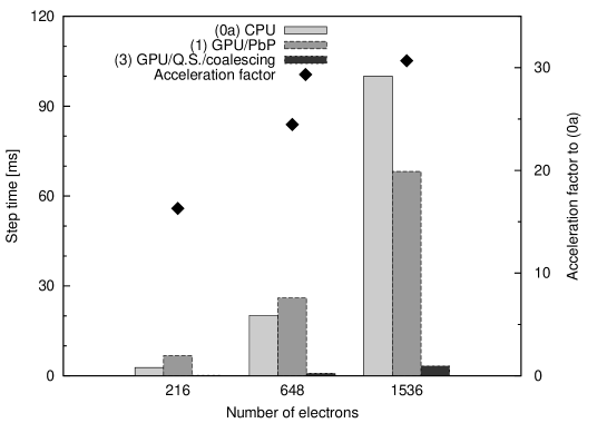
Figure 5: Computational time [ms] per MC step and corresponding acceleration factors for system sizes $N$ (number of electrons). ‘PbP’ and ‘Q.S.’ stand for the particle-by-particle and quasi-simultaneous updating schemes, respectively.

As mentioned in §IV.A, the number of parallelized threads scales as $(N\times L)\sim N^{2}$, so that the efficiency of the GPU improves for larger systems. Coalescing in implementation (3) also becomes more effective for larger $L$. However there is a drawback for larger systems in the data transfer costs, especially for returning $\left\{{\left\{{{\psi_{l}}\left({{{\vec{r}}_{i}}}\right)}\right\}_{i=1}^{N}}\right\}_{l=1}^{L}$ from the GPU to CPU. As overall cancellation, the acceleration seems to scale as $\sim N$ , rather than $\sim N^{2}$ (the number of threads).

Table 11: Data transfer costs between the CPU and GPU from implementation (3) in Table 7. The dependence on the system size $N$ (number of electrons) is shown.

	CPU $\to$ GPU ($\mu$s)		GPU $\to$ CPU ($\mu$s)	Total	Percentage
$N$	$s\left(\vec{r}^{\prime}_{j}\right)$	$\Theta_{s\left(\vec{r}^{\prime}_{j}\right)}\left(\vec{r}^{\prime}_{j}\right)$	$\psi_{l}\left(\vec{r}^{\prime}_{j}\right)$	($\mu$s)	within total GPU time
216	16.8	19.5	29.1	71.9	47.6 %
648	18.8	32.0	290.9	405.1	45.8 %
1,536	25.5	131.1	1046.6	1203.2	36.9 %

Table 11 summarizes the data transfer times using ver. (3), which show that the transfer cost increases with system size. The percentage of the total GPU time is, however, decreased because the number of GPU operations also increases.

Another remarkable fact illustrated by Fig. 5 is that the performance of ver. (1) is inferior up to $N$ = 648 but superior for larger $N$ = 1,536. The only possible reason for that is the concealment of memory latency, because in this implementation there is no coalescing and the operation load on each thread is simply a multiplication, although it has the largest number of warps among all the implementations.

VI Discussions

To prevent redundancy we omit discussions of the evaluation of how much of the original CPU code is optimized, and of how we interpret the acceleration factors achieved in terms of the actual usefulness of GPGPU, as these were discussed in our previous report UEJ11 .

VI.1 Acceleration performance

The ideal limit of the acceleration factor to be compared with our achievement of 30.7 is that of (1345/10.64)=126.4, where 1345 [GFlops] is the ideal limit for the GPU discussed in §III.A and 10.64 is the single core performance of the Intel Core i7 processor used here for implementation (0a). This limit might be achieved when the ratio of the cost of memory loads to that for operations approaches zero, although this is not possible in practice. This ratio corresponds to those shown in the last column of Table 11 as in percentages. As shown in the table, the ratio is decreased for larger systems and hence we expect better performance.

As another evaluation of our achievement, we estimated the FLOPS of our implementations applied to TiO₂ ($N$=1,536) as listed in Table 12. The values are obtained from the number of operations required only for Eq. (6) [(2 operations) $\times$ (2 components in complex numbers) per term] divided by the time taken for the GPU kernel execution. We did not take into account the operations required to identify which subset $\left\{s\right\}_{s=1}^{4^{3}}\subset\left\{\tilde{s}\right\}_{\tilde{s}=1}^{S=50^{3}\sim 60^{3}}$ should be chosen to form the coefficients $\left\{a_{ls}\right\}$. The actual FLOPS should therefore be larger than those given in the table.

Table 12: Estimated FLOPS for each implementation and the ratios to the ideal performances. ‘PbP’ and ‘Q.S.’ stand for the particle-by-particle and quasi-simultaneous updating schemes, respectively.

	Performance (GFlops)	Ratio to Ideal performance
(0a) CPU/PbP	1.50	14.10 %
(1) GPU/PbP	4.62	0.34 %
(2) GPU/Q.S./non-coalescing	9.05	0.71 %
(3) GPU/Q.S./coalescing	73.98	5.50 %

In this evaluation, our achievement of a factor 30.7 gives an efficiency of only 5.5% of the ideal performance. For reference, the CUBLAS (GPGPU of BLAS Level 3) is known to give 400 GFlops on the NVIDIA Tesla C2050, which is 38.8% of the peak performance tesla-blas . The reason for the lower percentage in our case is the smaller number of operations per thread, 64 terms multiply and add summations for (3), and just a single multiplication for (1) and (2). The amount does not depend on the system size because of the use of a localized spline basis set, although this is a disadvantage for GPGPU in the sense that the number of operations is smaller.

VI.2 Performances in memory access

Table 13 summarizes the memory load performances of each implementation as measured by ‘Compute Visual Profiler’ for CUDA profiler .

Table 13: Performance in global memory access for each implementation. ‘PbP’ and ‘Q.S.’ stand for the particle-by-particle and quasi-simultaneous updating schemes, respectively.

	Global Memory Access		SM activity
	Num. of 32bit Load	Throughput (GB/s)
(1) GPU/PbP	24,576	13.5	88.1 %
(2) GPU/Q.S./non-coalescing	188,744,000	18.1	99.4 %
(3) GPU/Q.S./coalescing	7,077,890	153.0	100.0 %

The increase in the number of 32 bit load from (1) to (2) is simply because of the increased number of threads due to the simultaneous processing with respect to the number of particles $N$ in Q.S. From the coalescing in (3) we see a remarkable reduction in the number of memory loads by a factor of $\sim$ 27. Correspondingly the throughput becomes much closer to the peak value, 177.4 GB/s, compared with the poor achievements in (1) and (2) due to the random access of $\left\{a_{js}\right\}$.

The SM activity in Table 13 is a measure of the efficiency of the concealment of the memory latency. This quantity is defined as the ratio of the number of cycles at which the operations started after the completion of memory loads to the total number of cycles taken for the kernel execution. With efficient concealing, at least one of the threads is always ready for execution at each cycle, and hence this quantity is expected to be close to 100%. Since the concealment becomes more effective with larger numbers of warps, the SM activity is increased from (1) to (2) by the increased number of threads. Though the number is decreased again in (3) by a factor of $\sim$ 64, greatly accelerated memory accesses by the coalescing improve the SM activity to 100%.

VI.3 Shared memory and read only memory

In our previous work UEJ11 we found that it was quite effective to exploit high-speed read-only memory. In the present work we have investigated further improvements by exploiting high-speed read-only memory but found no significant gains. This is summarized as follows: (i) in the present case the data required for the operation on each thread is large and does not fit into the high-speed memory devices, and (ii) even without explicit use of high-speed devices, the compiler automatically assigns them to L1 cache, and the explicit data transfer to shared memory by the user gives rather slower performance than automatic assignment.

The data loads considered in the present case are $\left\{{{{\tilde{a}}_{l,\tilde{s}}}}\right\}_{\tilde{s}=1}^{{S\sim 250,000}}$, which is initially stored in the global memory. After choosing the subset $\left\{\left\{{a_{l,s}}\right\}_{s=1}^{64}\right\}_{l=1}^{L}$ from $\left\{{{{\tilde{a}}_{l,\tilde{s}}}}\right\}$, our best implementation (3) loads them by coalescing access to the global memory. However, the access speed to the on-chip shared memory is around 100 times faster than that. . A block sharing a shared memory device has a common $j$ so the set $\left\{\left\{{a_{l,s}}\right\}_{s=1}^{64}\right\}_{l=1}^{L}$ is shared by all the threads within the block. The 64 KB capacity of the device corresponds to 16,000 (= 64 KB/4B) elements of single precision data. It is therefore possible to accommodate $\left\{{a_{l,s}}\right\}$ when $L<16,000/64=250$, so that the total number of orbitals is less than 250. Table 2 shows that Si ($3\times 3\times 3$) and TiO₂ ($3\times 3\times 3$) correspond to this case. Storing the data within the on-chip memories becomes advantageous when the data is referenced repeatedly by the warps. The number of repeated references is given in our case by the ratio of $L\sim$ 250 to the warp size, 32, which is less than 10. Beyond this number of repeats the SM switches to another process with different $j$ and hence the corresponding new data for $\left\{{a_{l,s}}\right\}$ should be loaded again from the global memory. We have tried such an implementation using shared memory devices but we did not find any improvements over (3), possibly because of the small number of repeated references. Such an improvement would already be included implicitly in (3) by L1 cache acting on the shared device. The explicit usage of the device as the shared memory seems to reduce the performance.

Another choice is to use constant memory. Unlike shared memory it is located off chip and blocks with different $j$ indices pick up their subset $\left\{{a_{l,s}}\right\}$. The memory should therefore be able to provide the whole set of $\left\{{{{\tilde{a}}_{l,\tilde{s}}}}\right\}$, which is far beyond the size of the constant memory and is therefore infeasible. Another data required for the GPU operation is $\left\{\left\{{\Theta_{s}\left({\vec{r}_{j}}\right)}\right\}_{j=1}^{N}\right\}_{s=1}^{64}$ in Eq. (6), the total size of which can be accommodated within the constant memory for $N<$ 250. Our trial implementation using constant memory for $\left\{\Theta_{s}\right\}$ actually gives a slight improvement in performance, by $\sim$ 4%, but this is only applicable to smaller system sizes. The data $\left\{{\Theta_{s}\left({\vec{r}_{j}^{(k)}}\right)}\right\}_{j=1}^{N}$ is updated at every MC step and hence the life time in cache is short, giving only a slight improvement in performance.

VI.4 Acceleration of Slater Determinant Updating

The bottleneck operation of updating of orbital functions, which are computed by the GPU, gives a system size dependence of $O(N^{2})$ NEE10 . The corresponding updating of the many-body wave function, (5), actually takes $O(N^{2})$ in the PbP implementation HAM94 ; CEP77 , in spite of the fact that evaluating a determinant scales as $O(N^{3})$. In PbP, say $\vec{r}_{j}\to\vec{r}^{\prime}_{j}$, only one column of the determinant including $\vec{r}^{\prime}_{j}$ is updated at each step. The updating of the determinant can hence be evaluated based on the Laplace expansion with respect to the column, and the other co-factors are unchanged. This algorithm, known as Sherman-Morrison updating CEP77 therefore requires only $O(N^{2})$ operations NEE10 . In our Q.S., the updated orbitals are stored in an array and are read sequentially to update the determinant using this algorithm. The cost of the updating of the many-body wave function amounts to 19.4% of the time compared to 39.5 % for the present bottleneck, the orbital updating, when $N$=1,536, dcorr=1. The ratio of the former to the latter increases with larger dcorr. This operation mostly involves BLAS routines (ddot and daxpy) which could be replaced by CUBLAS in future work.

VI.5 As a prototype of linear algebra problems

The evaluation of Eq. (6) can be written in terms of linear algebra,

$$\left({\begin{array}[]{*{20}{c}}{\psi_{1}\left({{{\vec{r}}_{j}}}\right)}\\ {\psi_{2}\left({{{\vec{r}}_{j}}}\right)}\\ \vdots\\ {\psi_{L}\left({{{\vec{r}}_{j}}}\right)}\end{array}}\right)=A\left({{{\vec{r}}_{j}}}\right)\cdot\left({\begin{array}[]{*{20}{c}}{{\Theta_{1}}\left({{{\vec{r}}_{j}}}\right)}\\ {{\Theta_{2}}\left({{{\vec{r}}_{j}}}\right)}\\ \vdots\\ {{\Theta_{64}}\left({{{\vec{r}}_{j}}}\right)}\end{array}}\right)\ ,$$ (13)

for which the matrix $A$ is defined by

$$A=\left\{{{a_{ls}}}\right\}=\left\{{{a_{l,s\left({{{\vec{r}}_{j}}}\right)}}}\right\}=A\left({{{\vec{r}}_{j}}}\right)\ .$$ (14)

If the matrix $A$ is constant, we can write Eq. (13) as a matrix multiplication:

$$\left({\begin{array}[]{*{20}{c}}{\psi_{1}\left({{{\vec{r}}_{1}}}\right)}&{\psi_{1}\left({{{\vec{r}}_{2}}}\right)}&\cdots&{\psi_{1}\left({{{\vec{r}}_{N}}}\right)}\\ {\psi_{2}\left({{{\vec{r}}_{1}}}\right)}&\ddots&&\vdots\\ \vdots&{}\hfil&{}\hfil&{}\hfil\\ {\psi_{L}\left({{{\vec{r}}_{1}}}\right)}&\cdots&{}\hfil&{\psi_{L}\left({{{\vec{r}}_{N}}}\right)}\end{array}}\right)=A\cdot\left({\begin{array}[]{*{20}{c}}{{\Theta_{1}}\left({{{\vec{r}}_{1}}}\right)}&{{\Theta_{1}}\left({{{\vec{r}}_{2}}}\right)}&\cdots&{{\Theta_{1}}\left({{{\vec{r}}_{N}}}\right)}\\ {{\Theta_{2}}\left({{{\vec{r}}_{1}}}\right)}&\ddots&{}\hfil&\vdots\\ \vdots&&&\\ {{\Theta_{64}}\left({{{\vec{r}}_{1}}}\right)}&\cdots&{}\hfil&{{\Theta_{64}}\left({{{\vec{r}}_{N}}}\right)}\end{array}}\right)\ ,$$ (15)

and using this we could increase the ratio of operations to data transfer, and hence the efficiency of GPGPU by a large amount. Fig. 1, however, reminds us that the matrix $A$ in Eq. (14) is randomly varying in its elements choice indexed by $\vec{r}_{j}$, but within the given constant elements $\left\{{{{\tilde{a}}_{l,\tilde{s}}}}\right\}$, and hence we cannot reduce Eq. (13) into a unified form as Eq. (15).

Since our calculation of Eq. (6) is linear algebra we considered whether it could be performed efficiently using CUBLAS. To use CUBLAS we have to construct $A\left({{{\vec{r}}_{j}}}\right)$ on the CPU at every MC step, transfer it to the GPU, and then call CUBLAS. In our case the randomly varying matrix $A$ is not large, however, the cost of constructing it cannot be compensated by the high performance of CUBLAS. Since the enlarged matrix $\tilde{A}=\left\{{{\tilde{a}_{l\tilde{s}}}}\right\}_{\tilde{s}=1}^{{S}}$ is a constant matrix, only one data transfer to the GPU is required in principle, but this is not possible with CUBLAS which requires the operands to be transferred every time for the operations. In this sense, our achievement here corresponds to an effective GPGPU implementation of the algorithm for the prototype as explained above, Eq. (13) with a randomly chosen matrix.

VII Concluding Remarks

We have applied GPGPU to the evaluation of the orbital functions in ab-initio Quantum Monte Carlo electronic structure calculations, which we identified as the computational bottleneck. For efficiency we propose a new updating scheme for generating trial moves for the walkers in the Monte Carlo sampling, which we call quasi-simultaneous updating. Using this scheme we achieved a speedup of more than a factor of 30 compared with using a single core CPU. The GPGPU implementation gives a deviation in energy from original CPU evaluation which is smaller that the required chemical accuracy. Though the effective performance in operations amounts to 74 GFlops, which is only 5.5% of the peak performance, the memory throughput reaches 153 GB/s, which is 86% of the peak value with almost perfect concealment of memory latency as shown by the SM activity. The implementation presented here is a prototypical problem of linear algebra with a sort of random matrix, processed by GPGPU.

VIII Acknowledgments

RM is grateful for financial support provided by a Grant in Aid for Scientific Research on Innovative Areas “Materials Design through Computics: Complex Correlation and Non-Equilibrium Dynamics” (Grant No. 22104011), and “Optical Science of Dynamically Correlated Electrons” (Grant No. 23104714) of the Ministry of Education, Culture, Sports, Science, and Technology (KAKENHI-MEXT/Japan). The authors would like to express our special thanks to Richard J. Needs and Kenta Hongo for their useful comments and kind supports for us.

References

-
(1)
“ gACM Workshop on General Purpose Computing on Graphics Processors” C
http://www.cs.unc.edu/Events/Conferences/GP2/ C Aug. 2004 - (2) W. Hwu, ‘GPU Computing Gems’, Morgan Kaufmann (2010).
- (3) J. Sanders and E. Kandrot, ‘CUDA by Example: An Introduction to General-Purpose GPU Programming’, Addison-Wesley (2010).
- (4) David B. Kirk and Wen-mei Hwu, ‘Programming Massively Parallel Processors: A Hands-on Approach’, Morgan Kaufmann (2010).
- (5) R.M. Martin, Electronic Structure, Cambridge University Press (2004).
- (6) R.J. Needs, M.D. Towler, N.D. Drummond and P. Lopez Rios, J. Phys. Condensed Matter 22, 023201 (2010).
- (7) B.L. Hammond, W.A. Lester, Jr., and P.J. Reynolds, Monte Carlo Methods in Ab Initio Quantum Chemistry; World Scientific: Singapore (1994).
- (8) N.D. Drummond and R.J. Needs, Phys. Rev. B 72, 085124 (2005).
- (9) P.R.C. Kent, R.J. Needs and G. Rajagopal Phys. Rev. B 59, 12344 (1999).
- (10) W.M.C. Foulkes, L. Mitas, R.J. Needs and G. Rajagopal, Rev. Mod. Phys. 73, 33 (2001).
- (11) M.J. Gillan, M.D. Towler and D. Alfé, Psi-k Highlight of the Month (February, 2011).
- (12) Y. Uejima, T. Terashima and R. Maezono, J. Comput. Chem. 32, 2264-2272 (2011).
- (13) K.P. Esler, J. Kim, L. Shulenburger and D.M. Ceperley, Computing in Science and Engineering 14, 40 (2012).
- (14) R. Maezono, H. Watanabe, Tanaka, M.D. Towler and R.J. Needs, J. Phys. Soc. Jpn. 76, 064301:1-5 (2007).
- (15) R.G. Parr and W. Yang, ‘Density-Functional Theory of Atoms and Molecules’, Oxford University Press (1994).
- (16) R.J. Jastrow, Phys. Rev. 98, 1479 (1955).
- (17) N.D. Drummond, M.D. Towler and R.J. Needs, Phys. Rev. B 70, 235119 (2004).
- (18) N.W. Ashcroft and N.D. Mermin, Solid State Physics (Thomson Learning, 1976).
- (19) R. Maezono, J. Comput. Theor. Nanosci. 6, 2474 (2009).
- (20) D. Alfé and M.J. Gillan, Phys. Rev. B 70, 161101 (2004).
- (21) R. Maezono, N.D. Drummond, A. Ma, and R.J. Needs, Phys. Rev. B 82, 184108 (2010).
- (22) M. Abbasnejad, E. Shojaee, M.R. Mohammadizadeh, M. Alaei, and R. Maezono, Appl. Phys. Lett. 100, 261902 (2012).
-
(23)
Intel VTune Amplifier C
http://software.intel.com/en-us/articles/intel-vtune-amplifier-xe/ - (24) Kenta Hongo, Ryo Maezono and Kenich Miura, J. Comput. Chem. 31, 2186 (2010).
- (25) Intel Core i7-920 Processor, http://ark.intel.com/Product.aspx?id=37147
-
(26)
Intel Hyper-Threading Technology C
http://www.intel.com/jp/technology/platform-technology/hyper-threading/index.htm -
(27)
Tesla C2050 Performance Benchmarks,
http://www.siliconmechanics.com/files/C2050Benchmarks.pdf, accessed on 1 Feb. 2012 -
(28)
NVIDIA Compute Visual Profiler C
http://developer.nvidia.com/nvidia-visual-profiler - (29) D.M. Ceperley, G.V. Chester and M.H. Kalos, Phys. Rev. B 16, 3081 (1977).