Numerical Invariants through Convex Relaxation and Max-Strategy Iteration

Abstract

In this article we develop a max-strategy improvement algorithm for computing least fixpoints of operators on ${\overline{\mathbb{R}}}^{n}$ (with ${\overline{\mathbb{R}}}:=\mathbb{R}\cup\{\pm\infty\}$) that are point-wise maxima of finitely many monotone and order-concave operators. Computing the uniquely determined least fixpoint of such operators is a problem that occurs frequently in the context of numerical program/systems verification/analysis. As an example for an application we discuss how our algorithm can be applied to compute numerical invariants of programs by abstract interpretation based on quadratic templates.

1 Introduction

1.1 Motivation

Finding tight invariants for a given program or system is crucial for many applications related to program respectively system verification. Examples include linear recursive filters and numerical integration schemes. Abstract Interpretation as introduced by Cousot and Cousot [4] reduces the problem of finding tight invariants to the problem of finding the uniquely determined least fixpoint of a monotone operator. In this article, we consider the problem of inferring numerical invariants using abstract domains that are based on templates. That is, in addition to the program or system we want to analyze, a set of templates is given. These templates are arithmetic expressions in the program/system variables. The goal then is to compute small safe upper bounds on these templates. We may, for instance, be interested in computing a safe upper bound on the difference ${\bf x}_{1}-{\bf x}_{2}$ of two program/system variables ${\bf x}_{1}$, ${\bf x}_{2}$ (at some specified control point of the program). Examples for template-based numerical invariants include intervals (upper and lower bounds on the values of the numerical program variables) [3], zones (intervals and additionally upper and lower bounds on the differences of program variables) [10, 18, 11], octagons (zones and additionally upper und lower bounds on the sum of program variables) [12], and, more generally, linear templates (also called template polyhedra, upper bounds on arbitrary linear functions in the program variables, where the functions a given a priori) [15]. In this article, we focus on quadratic templates as considered by Adjé, Gaubert, and Goubault [1]. That is, a priori, a set of linear and quadratic functions in the program variables (the templates) is given and we are interested in computing small upper bounds on the values of these functions. An example for a quadratic template is represented by the quadratic polynomial $2x_{1}^{2}+3x_{2}^{2}+2x_{1}x_{2}$, where $x_{1}$ and $x_{2}$ are program variables.

When using such a template-based numerical abstract domain, the problem of finding the minimal inductive invariant, that can be expressed in the abstract domain specified by the templates, can be recast as a purely mathematical optimization problem, where the goal is to minimize a vector $({\bf x}_{1},\ldots,{\bf x}_{n})$ subject to a set of inequalities of the form

$${\bf x}_{i}\geq f({\bf x}_{1},\ldots,{\bf x}_{n}).$$ (1)

Here, $f$ is a monotone operator. The variables ${\bf x}_{1},\ldots,{\bf x}_{n}$ take values in $\mathbb{R}\cup\{\pm\infty\}$. The variables are representing upper bounds on the values of the templates. Accordingly, the vector $({\bf x}_{1},\ldots,{\bf x}_{n})$ is to be minimized w.r.t. the usual component-wise ordering. Because of the monotonicity of the operators $f$ occurring in the right-hand sides of the inequalities and the completeness of the linearly ordered set $\mathbb{R}\cup\{\pm\infty\}$, the fixpoint theorem of Knaster/Tarski ensures the existence of a uniquely determined least solution.

Computing the least solution of such a constraint system is a difficult task. Even if we restrict our consideration to the special case of intervals as an abstract domain, which is, if the program variables are denoted by $x_{1},\ldots,x_{n}$, specified by the templates $-x_{1},x_{1},\ldots,-x_{n},x_{n}$, the static analysis problem is at least as hard as solving mean payoff games. The latter problem is a long outstanding problem which is in $\mathsf{NP}$ and in $\mathsf{coNP}$, but not known to be in $\mathsf{P}$.

A generic way of solving systems of constraints of the form (1) with right-hand sides that are monotone and variables that range over a complete lattice is given through the abstract interpretation framework of Cousot and Cousot [4]. Solving constraint systems in this framework is based on Kleene fixpoint iteration. However, in our case the lattice has infinite ascending chains. In this case, termination of the fixpoint iteration is ensured through an appropriate widening (see Cousot and Cousot [4]). Widening, however, buys termination for precision. Although the lost precision can be partially recovered through a subsequently performed narrowing iteration, there is no guarantee that the computed result is minimal.

1.2 Main Contribution

In this article, we study the case where the operators $f$ in the right-hand side of the systems of equations of the form (1) are not only monotone, but additionally order-concave or even concave (concavity implies order-concavity, but not vice-versa). In the static program analysis application we consider in this article, the end up in this comfortable situation by considering a semi-definite relaxation of the abstract semantics. The concavity of the mappings $f$, however, does not imply that the problem can be formulated as a convex optimization problem. The feasible space of the resulting mathematical optimization problem is normally neither order-convex nor order-concave and thus neither convex nor concave. In consequence, convex optimization methods cannot be directly applied. For the linear case (obtained when using used linear templates), we solved a long outstanding problem — namely the problem of solving mean payoff games in polynomial time — if we would be able to formalize the problem through a linear programming problem that can be constructed in polynomial time.

In this article, we exploit the fact that the operators $f$ that occur in the right-hand sides of the system of inequalities of the form (1) we have to solve are not only order-concave, but also monotone. In other words: we do not require convexity of the feasible space, but we do require monotonicity in addition to the order-concavity. The main contribution of this article is an algorithm for computing least solutions of such systems of inequalities. The algorithm is based on strategy iteration. That is, we consider the process of solving the system of inequality as a game between a maximizer and a minimizer. The maximizer aims at minimizing the solution, whereas the minimizer aims at minimizing it. The algorithm iteratively constructs a winning strategy for the maximizer — a so-called max-strategy. It uses convex optimization techniques as sub-routines to evaluate parts of the constructed max-strategy. The concrete convex optimization technique that is used for the evaluation depends on the right-hand sides. In some cases linear programming is sufficient (see Gawlitza and Seidl [5, 8]), In other cases more sophisticated convex optimization techniques are required. The application we study in this article will require semi-definite programming.

An important example for monotone and order-concave operators are the operators that are monotone and affine. The class of monotone and order-concave operators is closed under the point-wise infimum operator. The point-wise infimum of a set of monotone and affine functions, for instance, is monotone and order-concave. Another example is the $\sqrt{\phantom{x}}$-operator, which is defined by $\sqrt{x}=\sup\;\{y\in\mathbb{R}\mid y^{2}\leq x\}$ for all $x\in{\overline{\mathbb{R}}}$.

An example for a system of inequalities of the class we are considering in this article is the following system of inequalities:

$${\bf x}_{1} \geq\frac{1}{2} {\bf x}_{1} \geq\sqrt{\bf x}_{2} {\bf x}_{2} \geq{\bf x}_{1} {\bf x}_{2} \geq 1+\sqrt{{\bf x}_{2}-1}$$ (2)

The uniquely determined least solution of the system (2) of inequalities is ${\bf x}_{1}={\bf x}_{2}=1$. We remind the reader again that the important property here is that the right-hand sides of (2) are monotone and order-concave.

The least solution of the system (2) is also the uniquely determined optimal solution of the following convex optimization problem:

$$\max\;\; {\bf x}_{1}+{\bf x}_{2} {\bf x}_{1} \leq\sqrt{\bf x}_{2} {\bf x}_{2} \leq{\bf x}_{1}$$ subject to (3)

Observe that the above convex optimization problem is in some sense a “subsystem” of the system (2). Such a “subsystem”, which we will call a max-strategy later on, is obtained from the system (2) by selecting exactly one inequality of the form ${\bf x}_{i}\geq e_{i}$ from (2) for each variable ${\bf x}_{i}$ and replacing the relation $\leq$ by the relation $\geq$. Note that there are exponentially many max-strategies. The algorithm we present in this article starts with a max-strategy and assigns a value to it. It then iteratively improves the current max-strategy and assigns a new value to it until the least solution is found. We utilize the monotonicity and the order-concavity of the right-hand sides to prove that our algorithm always terminates with the least solution after at most exponentially many improvement steps. Each improvement step can be executed by solving linearly many convex optimization problems, each of which can be constructed in linear time.

As a second contribution of this article, we show how any algorithm for solving such systems of inequalities, e.g., our max-strategy improvement algorithm, can be applied to infer numerical invariants based on quadratic templates. The method is based on the relaxed abstract semantics introduced by Adjé, Gaubert, and Goubault [1].

1.3 Related Work

The most closely related work is the work of Adjé, Gaubert, and Goubault [1]. They apply the min-strategy improvement approach of Costan, Gaubert, Goubault, Martel, and Putot [2] to the problem of inferring quadratic invariants of programs. In order to do so, they introduced the relaxed abstract semantics we are going to use in this article. Their method, however, has several drawbacks compared to the method we present in this article. The first drawback is that it does not necessarily terminate after finitely many steps. In addition, even if it terminates, the computed solution is not guaranteed to be minimal. On the other hand, their approach also has substantial advantages that are especially important in practice. Firstly, it can be stopped at any time with a safe over-approximation to the least solution. Secondly, the computational steps that have to be performed are quite cheap compared the the ones we have to perform for the method we propose in this article. This is caused by the fact that the semi-definite programming problems (or in more general cases: convex programming problems) that have to be solved in each iteration are reasonable small. We refer to Gawlitza, Seidl, Adjé, Gaubert, and Goubault [9] for a detailed comparison between the max- and the min-strategy approach.

1.4 Previous Publications

Parts of this work were previously published in the proceedings of the Seventeenth International Static Analysis Symposium (SAS 2010). In contrast to the latter version, this article contains the full proofs and the precise treatment of infinities. In order to simplify some argumentations and to deal with infinities, we modified some definitions quite substentially. In addition to these improvements, we provide a much more detailed study of different classes of order-concave functions and the consequences for our max-strategy improvement algorithm. We do not report on experimental results in this article. Such reports can be found in the article in the proceedings of the Seventeenth International Static Analysis Symposium (SAS 2010).

1.5 Structure

This article is structured as follows: Section 2 is dedicated to preliminaries. We study the class of monotone and order-concave operators in Section 3. The results we obtain in Section 3 are important to prove the correctness of our max-strategy improvement algorithm. The method and its correctness proof is presented in Section 4. In Section 5, we discuss the important special cases where the right-hand sides of the system of inequalities are parametrized convex optimization problems. This can be used to evaluate strategies more efficiently. These special cases are important, since they are present especially in the program analysis applications we mainly have in mind. In Section 6, we finally explain how our methods can be applied to a numerical static program analysis based on quadratic templates. We conclude with Section 7.

2 Preliminaries

Vectors and Matrices

We denote the $i$-th row (resp. $j$-th column) of a matrix $A$ by $A_{i\cdot}$ (resp. $A_{\cdot j}$). Accordingly, $A_{i\cdot j}$ denotes the component in the $i$-th row and the $j$-th column. We also use these notations for vectors and vector valued functions $f:X\to Y^{k}$, i.e., $f_{i\cdot}(x)=(f(x))_{i\cdot}$ for all $i\in\{1,\ldots,k\}$ and all $x\in X$.

Sets, Functions, and Partial Functions

We write $A\operatorname{{\dot{\cup}}}B$ for the disjoint union of the two sets $A$ and $B$, i.e., $A\operatorname{{\dot{\cup}}}B$ stands for $A\cup B$, where we assume that $A\cap B=\emptyset$. For sets $X$ and $Y$, $X\to Y$ denotes the set of all functions from $X$ to $Y$, and $X\rightsquigarrow Y$ denotes the set of all partial functions from $X$ to $Y$. Note that $X\to Y\subseteq X\rightsquigarrow Y\subseteq X\times Y$. Accordingly, we apply the set operators $\cup$, $\cap$, and $\setminus$ also to partial functions. For $X^{\prime}\subseteq X$, the restriction $f|_{X^{\prime}}:X^{\prime}\to Y$ of a function $f:X\to Y$ to $X^{\prime}$ is defined by $f|_{X^{\prime}}:=f\cap X^{\prime}\times Y$. The domain and the codomain of a partial function $f$ are denoted by $\operatorname{\mathsf{dom}}(f)$ and $\operatorname{\mathsf{codom}}(f)$, respectively. For $f:X\to Y$ and $g:X\rightsquigarrow Y$, we define $f\oplus g:X\to Y$ by $f\oplus g:=f|_{X\setminus\operatorname{\mathsf{dom}}(g)}\cup g$.

Partially Ordered Sets

Let $\mathbb{D}$ be a partially ordered set (partially ordered by the binary relation $\leq$). Two elements $x,y\in\mathbb{D}$ are called comparable if and only if $x\leq y$ or $y\leq x$. For all $x\in\mathbb{D}$, we set $\mathbb{D}_{\geq x}:=\{y\in\mathbb{D}\mid y\geq x\}$ and $\mathbb{D}_{\leq x}:=\{y\in\mathbb{D}\mid y\leq x\}$. We denote the least upper bound and the greatest lower bound of a set $X\subseteq\mathbb{D}$ by $\bigvee X$ and $\bigwedge X$, respectively, provided that it exists. The least element $\bigvee\emptyset=\bigwedge\mathbb{D}$ (resp. the greatest element $\bigwedge\emptyset=\bigvee\mathbb{D}$) is denoted by $\bot$ (resp. $\top$), provided that it exists. A subset $C\subseteq\mathbb{D}$ is called a chain if and only if $C$ is linearly ordered by $\leq$, i.e., it holds $x\leq y$ or $y\leq x$ for all $x,y\in C$. For every subset $X\subseteq\mathbb{D}$ of a set $\mathbb{D}$ that is partially ordered by $\leq$, we set $X{\uparrow^{\mathbb{D}}}:=\{y\in\mathbb{D}\mid\exists x\in X\,.\,x\leq y\}$. The set $X\subseteq\mathbb{D}$ is called upward closed w.r.t. $\mathbb{D}$ if and only if $X{\uparrow^{\mathbb{D}}}=X$. We omit the reference to $\mathbb{D}$, if $\mathbb{D}$ is clear from the context.

Monotonicity

Let $\mathbb{D}_{1},\mathbb{D}_{2}$ be partially ordered sets (partially ordered by $\leq$). A mapping $f:\mathbb{D}_{1}\to\mathbb{D}_{2}$ is called monotone if and only if $f(x)\leq f(y)$ for all $x,y\in\mathbb{D}_{1}$ with $x\leq y$. A monotone function $f$ is called upward-chain-continuous (resp. downward-chain-continuous) if and only if $f(\bigvee C)=\bigvee f(C)$ (resp. $f(\bigwedge C)=\bigwedge f(C)$) for every non-empty chain $C$ with $\bigvee C\in\operatorname{\mathsf{dom}}(f)$ (resp. $\bigwedge C\in\operatorname{\mathsf{dom}}(f)$). It is called chain-continuous if and only if it is upward-chain-continuous and downward-chain-continuous.

Complete Lattices

A partially ordered set $\mathbb{D}$ is called a complete lattice if and only if $\bigvee X$ and $\bigwedge X$ exist for all $X\subseteq\mathbb{D}$. If $\mathbb{D}$ is a complete lattice and $x\in\mathbb{D}$, then the sublattices $\mathbb{D}_{\geq x}$ and $\mathbb{D}_{\leq x}$ are also complete lattices. On a complete lattice $\mathbb{D}$, we define the binary operators $\vee$ and $\wedge$ by

$$x\vee y:=\bigvee\{x,y\}\text{ and }x\wedge y:=\bigwedge\{x,y\} \text{for all }x,y\in\mathbb{D},$$ (4)

respectively. If the complete lattice $\mathbb{D}$ is a complete linearly ordered set (for instance ${\overline{\mathbb{R}}}=\mathbb{R}\cup\{\pm\infty\}$), then $\vee$ is the binary maximum operator and $\wedge$ the binary minimum operator. For all binary operators $\Box\in\{\vee,\wedge\}$, we also consider $x_{1}\;\Box\;\cdots\;\Box\;x_{k}$ as the application of a $k$-ary operator. This will cause no problems, since the binary operators $\vee$ and $\wedge$ are associative and commutative.

Fixpoints

Assume that the set $\mathbb{D}$ is partially ordered by $\leq$ and $f:\mathbb{D}\to\mathbb{D}$ is a unary operator on $\mathbb{D}$. An element $x\in\mathbb{D}$ is called fixpoint (resp. pre-fixpoint, resp. post-fixpoint) of $f$ if and only if $x=f(x)$ (resp. $x\leq f(x)$, resp. $x\geq f(x)$). The set of all fixpoints (resp. pre-fixpoints, resp. post-fixpoints) of $f$ is denoted by $\mathbf{Fix}(f)$ (resp. $\mathbf{PreFix}(f)$, resp. $\mathbf{PostFix}(f)$). We denote the least (resp. greatest) fixpoint of $f$ — provided that it exists — by $\mu f$ (resp. $\nu f$). If the partially ordered set $\mathbb{D}$ is a complete lattice and $f$ is monotone, then the fixpoint theorem of Knaster/Tarski [16] ensures the existence of $\mu f$ and $\nu f$. Moreover, we have $\mu f=\bigwedge\mathbf{PostFix}(f)$ and dually $\nu f=\bigvee\mathbf{PreFix}(f)$.

We write $\mu_{\geq x}f$ (resp. $\nu_{\leq x}f$) for the least element in the set $\mathbf{Fix}(f)\cap\mathbb{D}_{\geq x}$ (resp. $\mathbf{Fix}(f)\cap\mathbb{D}_{\leq x}$). The existence of $\mu_{\geq x}f$ (resp. $\nu_{\leq x}f$) is ensured if $\mathbb{D}_{\geq x}$ is a complete lattice and $f|_{\mathbb{D}_{\geq x}}$ (resp. $f|_{\mathbb{D}_{\leq x}}$) is a monotone operator on $\mathbb{D}_{\geq x}$ (resp. $\mathbb{D}_{\leq x}$), i.e., if $\mathbb{D}_{\geq x}$ (resp. $\mathbb{D}_{\leq x}$) is closed under the operator $f$. The latter condition is, for instance, fulfilled if $\mathbb{D}$ is a complete lattice, $f$ is a monotone operator on $\mathbb{D}$, and $x$ is a pre-fixpoint (resp. post-fixpoint) of $f$.

The Complete Lattice ${\overline{\mathbb{R}}}^{n}$

The set of real numbers is denoted by $\mathbb{R}$, and the complete linearly ordered set $\mathbb{R}\cup\{\pm\infty\}$ is denoted by ${\overline{\mathbb{R}}}$. Therefore, the set ${\overline{\mathbb{R}}}^{n}$ is a complete lattice that is partially ordered by $\leq$, where we write $x\leq y$ if and only if $x_{i\cdot}\leq y_{i\cdot}$ for all $i\in\{1,\ldots,n\}$. As usual, we write $x<y$ if and only if $x\leq y$ and $x\neq y$. We write $x\lhd y$ if and only if $x_{i\cdot}<y_{i\cdot}$ for all $i\in\{1,\ldots,n\}$. For $f:{\overline{\mathbb{R}}}^{n}\rightsquigarrow{\overline{\mathbb{R}}}^{m}$, we set $\operatorname{\mathsf{fdom}}(f):=\{x\in\operatorname{\mathsf{dom}}(f)\cap\mathbb{R}^{n}\mid f(x)\in\mathbb{R}^{m}\}.$

The Vector Space $\mathbb{R}^{n}$

The standard base vectors of the Euclidian vector space $\mathbb{R}^{n}$ are denoted by $e_{1},\ldots,e_{n}$. We denote the maximum norm on $\mathbb{R}^{n}$ by $\left\|\cdot\right\|$, i.e., $\left\|x\right\|=\max\;\{\left|x_{i\cdot}\right|\mid i\in\{1,\ldots,n\}\}$ for all $x\in\mathbb{R}^{n}$. A vector $x\in\mathbb{R}^{n}$ with $\left\|x\right\|=1$ is called a unit vector.

3 Morcave Operators

In this section, we introduce a notion of order-concavity for functions from the set ${\overline{\mathbb{R}}}^{n}\to{\overline{\mathbb{R}}}^{m}$. We then study the properties of functions that are monotone and order-concave. The results obtained in this section are used in Section 4 to prove the correctness of our max-strategy improvement algorithm.

3.1 Monotone Operators on $\mathbb{R}^{n}$

In this subsection, we collect important properties about monotone operators on $\mathbb{R}^{n}$. We start with the following auxiliary lemma:

Lemma 1

Let $d,d^{\prime}\in\mathbb{R}^{n}$ with $d\rhd 0$ and $d^{\prime}\geq 0$. There exist $j\in\{1,\ldots,n\}$ and $\lambda,\lambda_{1},\ldots,\lambda_{n}\geq 0$ such that $\lambda_{j}=0$ and $\lambda d=d^{\prime}+\sum_{i=1}^{n}\lambda_{i}e_{i}$.

Proof.

Since $d\rhd 0$, there exist a $j\in\{1,\ldots,n\}$ and a $\lambda\geq 0$ such that $\lambda d-d^{\prime}\geq 0$ and $(\lambda d-d^{\prime})_{j\cdot}=0$. Thus, there exist $\lambda_{1},\ldots,\lambda_{n}$ with $\lambda_{j}=0$ such that $\lambda d-d^{\prime}=\sum_{i=1}^{n}\lambda_{i}e_{i}$. ∎∎

We now provide a sufficient criterium for a fixpoint $x$ of a monotone partial operator $f$ on $\mathbb{R}^{n}$ for being the greatest pre-fixpoint of $f$. Such sufficient criteria are crucial to prove the correctness of our max-strategy improvement algorithm.

Lemma 2

Let $f:\mathbb{R}^{n}\rightsquigarrow\mathbb{R}^{n}$ be monotone with $\operatorname{\mathsf{dom}}(f)$ upward closed, $f(x)=x$, and $k\in\mathbb{N}$. Assume that, for every $\epsilon>0$, there exists a unit vector $d_{\epsilon}\rhd 0$ such that $f^{k}(x+\lambda d_{\epsilon})\lhd x+\lambda d_{\epsilon}$ for all $\lambda\geq\epsilon$. Then, $y\leq x$ for all $y$ with $y\leq f(y)$, i.e., $x$ is the greatest pre-fixpoint of $f$.

Proof.

We show $y\not\leq x\implies y\not\leq f(y)$. For that, we first show the following statement:

$$y>x\implies y\not\leq f(y)$$ (5)

For that, let $y>x$. Let $\epsilon:=\left\|y-x\right\|$. By Lemma 1, there exist $\lambda,\lambda_{1},\ldots,\lambda_{n}\geq 0$ with $\lambda_{j}=0$ for some $j\in\{1,\ldots,n\}$ such that $\overline{y}:=x+\lambda d_{\epsilon}=y+\sum_{i=1}^{n}\lambda_{i}e_{i}$ holds. We necessarily have $\lambda\geq\epsilon$. Using the monotonicity of $f$ and the fact that $f^{k}(\overline{y})\lhd\overline{y}$ holds by assumption, we get $f^{k}_{j\cdot}(y)\leq f^{k}_{j\cdot}(\overline{y})<\overline{y}_{j\cdot}=y_{j\cdot}$. Therefore, $y\not\leq f(y)$. Thus, we have shown (5). Now, let $y\not\leq x$. Thus, $y^{\prime}:=x\vee y>x$. Using (5) we get $y^{\prime}\not\leq f(y^{\prime})$. For the sake of contradiction assume that $y\leq f(y)$ holds. Then we get $f(y^{\prime})=f(x\vee y)\geq f(x)\vee f(y)\geq x\vee y=y^{\prime}$ — contradiction. ∎∎

In the remainder of this article, we only use the following corollary of Lemma 2:

Lemma 3

Let $f:\mathbb{R}^{n}\rightsquigarrow\mathbb{R}^{n}$ be monotone with $\operatorname{\mathsf{dom}}(f)$ upward closed, $f(x)=x$, and $k\in\mathbb{N}$. Assume that there exists a unit vector $d\rhd 0$ such that $f^{k}(x+\lambda d)\lhd x+\lambda d$ for all $\lambda>0$. Then, $y\leq x$ for all $y$ with $y\leq f(y)$, i.e., $x$ is the greatest pre-fixpoint of $f$. ∎

3.2 Monotone and Order-Concave Operators on $\mathbb{R}^{n}$

A set $X\subseteq\mathbb{R}^{n}$ is called order-convex if and only if $\lambda x+(1-\lambda)y\in X$ for all comparable $x,y\in X$ and all $\lambda\in[0,1]$. It is called convex if and only if this condition holds for all $x,y\in X$. Every convex set is order-convex, but not vice-versa. If $n=1$, then every order-convex set is convex. Every upward closed set is order-convex, but not necessarily convex.

A partial function $f:\mathbb{R}^{n}\rightsquigarrow\mathbb{R}^{m}$ is called order-convex (resp. order-concave) if and only if $\operatorname{\mathsf{dom}}(f)$ is order-convex and

$$f(\lambda x+(1-\lambda)y)\leq\text{(resp.\ $\geq$)}\;\lambda f(x)+(1-\lambda)f(y)$$ (6)

for all comparable $x,y\in\operatorname{\mathsf{dom}}(f)$ and all $\lambda\in[0,1]$ (cf. Ortega and Rheinboldt [14]). A partial function $f:\mathbb{R}^{n}\rightsquigarrow\mathbb{R}^{m}$ is called convex (resp. concave) if and only if $\operatorname{\mathsf{dom}}(f)$ is convex and

$$f(\lambda x+(1-\lambda)y)\leq\text{(resp.\ $\geq$)}\;\lambda f(x)+(1-\lambda)f(y)$$ (7)

for all $x,y\in\operatorname{\mathsf{dom}}(f)$ and all $\lambda\in[0,1]$ (cf. Ortega and Rheinboldt [14]). Every convex (resp. concave) partial function is order-convex (resp. order-concave), but not vice-versa. Note that $f$ is (order-)concave if and only if $-f$ is (order-)convex. Note also that $f$ is (order-)convex (resp. (order-)concave) if and only if $f_{i\cdot}$ is (order-)convex (resp. (order-)concave) for all $i=1,\ldots,m$. If $n=1$, then every order-convex (resp. order-concave) partial function is convex (resp. concave). Every order-convex/order-concave partial function is chain-continuous. Every convex/concave partial function is continuous.

The set of (order-)convex (resp. (order-)concave) partial functions is not closed under composition. The functions $f,g$ defined by $f(x)=(x-2)^{2}$ and $g(x)=\frac{1}{x}$ for all $x\in\mathbb{R}_{>0}$, for instance, are both convex and thus also order-convex. However, $f\circ g$ with $(f\circ g)(x)=(\frac{1}{x}-2)^{2}$ for all $x\in\mathbb{R}_{>0}$ is neither convex nor order-convex.

In contrast to the set of all order-concave partial functions, the set of all partial functions that are monotone and order-concave is closed under composition:

Lemma 4

Let $f:\mathbb{R}^{m}\rightsquigarrow\mathbb{R}^{n}$ and $g:\mathbb{R}^{l}\rightsquigarrow\mathbb{R}^{m}$ be monotone and order-convex (resp. order-concave). Assume that $\operatorname{\mathsf{codom}}(g)\subseteq\operatorname{\mathsf{dom}}(f)$. Then $f\circ g$ is monotone and order-convex (resp. order-concave).

Proof.

We assume that $f$ and $g$ are order-convex. The other case can be proven dually. Let $x,x^{\prime}\in\operatorname{\mathsf{dom}}(g)$ with $x\leq x^{\prime}$, $y=g(x)$, $y^{\prime}=g(x^{\prime})$. Since $g$ is monotone, we get $y\leq y^{\prime}$. Since $f$ is monotone, we get $(f\circ g)(x)=f(g(x))=f(y)\leq f(y^{\prime})=f(g(x^{\prime}))=(f\circ g)(x^{\prime})$. Hence, $f\circ g$ is monotone.

Let $\lambda\in[0,1]$. Then $(f\circ g)(\lambda x+(1-\lambda)x^{\prime})=f(g(\lambda x+(1-\lambda)x^{\prime})\leq f(\lambda g(x)+(1-\lambda)g(x^{\prime}))=f(\lambda y+(1-\lambda)y^{\prime})\leq\lambda f(y)+(1-\lambda)f(y^{\prime})=\lambda f(g(x))+(1-\lambda)f(g(x^{\prime}))=\lambda(f\circ g)(x)+(1-\lambda)(f\circ g)(x^{\prime})$, because $f$ is monotone, and $f$ and $g$ are order-convex. Hence, $f\circ g$ is order-convex. ∎∎

3.3 Fixpoints of Monotone and Order-concave Operators on $\mathbb{R}^{n}$

We now study the fixpoints of monotone and order-concave partial operators on $\mathbb{R}^{n}$. We are in particular interested in developing a simple sufficient criterium for a fixpoint of a monotone and order-concave partial operator on $\mathbb{R}^{n}$ for being the greatest pre-fixpoint of this partial operator. To prepare this, we first show the following lemma:

Lemma 5

Let $f:\mathbb{R}^{n}\rightsquigarrow\mathbb{R}^{n}$ be order-convex (resp. order-concave). Let $x,x^{*}\in\operatorname{\mathsf{dom}}(f)$ with $x^{*}=f(x^{*})$, $x\rhd\text{(resp.\ $\lhd$)}\,f(x)$, $d:=x^{*}-x\rhd 0$. Then, $x^{*}+\lambda d\lhd\text{(resp.\ $\rhd$)}\,f(x^{*}+\lambda d)$ for all $\lambda>0$ with $x^{*}+\lambda d\in\operatorname{\mathsf{dom}}(f)$.

Proof.

We only consider the case that $f$ is order-convex. The proof for the case that $f$ is order-concave can be carried out dually. Let $\lambda>0$. Assume for the sake of contradiction that there exists some $i\in\{1,\ldots,n\}$ such that $(x^{*}+\lambda d)_{i\cdot}\geq f_{i\cdot}(x^{*}+\lambda d)$. Since $f_{i\cdot}$ is order-convex and $x_{i\cdot}>f_{i\cdot}(x)$ holds, it follows $x^{*}_{i\cdot}>f_{i\cdot}(x^{*})$ — contradiction. ∎∎

We now use the results obtained so far to prove the following sufficient criterium for a fixpoint of a monotone and order-concave partial operator for being the greatest pre-fixpoint.

Lemma 6

Let $f:\mathbb{R}^{n}\rightsquigarrow\mathbb{R}^{n}$ be monotone and order-concave with $\operatorname{\mathsf{dom}}(f)$ upward closed. Let $x^{*}$ be a fixpoint of $f$, $x$ be a pre-fixpoint of $f$ with $x\lhd x^{*}$, and $\mu_{\geq x}f=x^{*}$. Then, $x^{*}$ is the greatest pre-fixpoint of $f$.

Proof.

Since $f$ is chain-continuous and $x\lhd x^{*}$ is a pre-fixpoint of $f$, there exists some $k\in\mathbb{N}$ such that $x\lhd f^{k}(x)$. Let $x^{\prime}$ be a pre-fixpoint of $f$. Let $d:=x^{*}-x$. Note that $d\rhd 0$. Since $f^{k}|_{\mathbb{R}^{n}_{\geq x}}=(f|_{\mathbb{R}^{n}_{\geq x}})^{k}$ is monotone and order-concave by Lemma 4, and $x^{*}$ is a fixpoint of $f^{k}$ and thus of $f^{k}|_{\mathbb{R}^{n}_{\geq x}}$, we get $f^{k}(x^{*}+\lambda d)=f^{k}|_{\mathbb{R}^{n}_{\geq x}}(x^{*}+\lambda d)\lhd x^{*}+\lambda d$ for all $\lambda\in\mathbb{R}_{>0}$ by Lemma 5. Thus, Lemma 3 gives us $x^{\prime}\leq x^{*}$. ∎∎

Example 1

Let us consider the monotone and concave partial operator $\sqrt{\cdot}:\mathbb{R}\rightsquigarrow\mathbb{R}$. The points $0$ and $1$ are fixpoints of $\sqrt{\cdot}$, since $0=\sqrt{0}$, and $1=\sqrt{1}$. Since $\frac{1}{2}$ is a pre-fixpoint of $\sqrt{\cdot}$, $\frac{1}{2}<1$, and $\mu_{\geq\frac{1}{2}}\sqrt{\cdot}=1$, Lemma 6 implies that $1$ is the greatest pre-fixpoint of $\sqrt{\cdot}$. Observe that for the fixpoint $0$, there is no pre-fixpoint $x\in\mathbb{R}$ of $\sqrt{\cdot}$ with $x<0$. Therefore, Lemma 6 cannot be applied. ∎

The following example shows that the criterium of Lemma 6 is sufficient, but not necessary:

Example 2

Let $f:\mathbb{R}\to\mathbb{R}$ be defined by $f(x)=0\wedge x$ for all $x\in\mathbb{R}$. Recall that $\wedge$ denotes the minimum operator. Then, $0$ is the greatest pre-fixpoint of $f$. However, there does not exist a $x\in\mathbb{R}$ with $x<0$ such that $\mu_{\geq x}f=0$, since $\mu_{\geq x}f=x$ for all $x\leq 0$. Therefore, Lemma 6 cannot be applied to show that $0$ is the greatest pre-fixpoint of $f$. ∎

The set $\mathbb{R}^{n}$ can be identified with the set $\{1,\ldots,n\}\to\mathbb{R}$ which can be identified with the set ${\bf X}\to\mathbb{R}$, whenever $\left|{\bf X}\right|=n$. In the remainder of this article, we therefore identify the set $({\bf X}\to\mathbb{R})\rightsquigarrow({\bf X}\to\mathbb{R})$ with the set $\mathbb{R}^{n}\rightsquigarrow\mathbb{R}^{n}$ — provided that $\left|{\bf X}\right|=n$. Usually, we use ${\bf X}=\{{\bf x}_{1},\ldots,{\bf x}_{n}\}$. We use one or the other representation depending on which representation is more convenient in the given context.

Our next goal is to weaken the preconditions of Lemma 6, i.e., we aim at providing a weaker sufficient criterium for a fixpoint of a monotone and order-concave partial operator for being the greatest pre-fixpoint than the one provided by Lemma 6. The weaker sufficient criterium we are going to develop can, for instance, be applied to the following example:

Example 3

Let us consider the monotone and order-concave partial operator $f:\mathbb{R}^{2}\rightsquigarrow\mathbb{R}^{2}$ defined by $f(x_{1},x_{2}):=(x_{2}+1\wedge 0,\;\sqrt{x}_{1})$ for all $x_{1},x_{2}\in\mathbb{R}$. Then, $x^{*}=(x^{*}_{1},x^{*}_{2})=(0,0)$ is the greatest pre-fixpoint of $f$. In order to prove this, assume that $y=(y_{1},y_{2})>x^{*}$ is a pre-fixpoint of $f$, i.e., $y_{1}\leq y_{2}+1$, $y_{1}\leq 0$, and $y_{2}\leq\sqrt{y_{1}}$. It follows immediately that $y_{1}\leq 0$ and thus $y_{2}\leq\sqrt{y_{1}}\leq\sqrt{0}=0$.

Lemma 6 is not applicable to prove that $x^{*}$ is the greatest pre-fixpoint of $f$, because there is no pre-fixpoint $x$ of $f$ with $x\lhd x^{*}$. The situation is even worse: there is no $x\in\operatorname{\mathsf{dom}}(f)$ with $x\lhd x^{*}$.

We observe that, locally at $x^{*}=(0,0)$, the first component $f_{1\cdot}$ of $f$ does not depend on the second argument in the following sense: For every $y=(y_{1},y_{2})\in\mathbb{R}^{2}$ with $y_{1}=x^{*}_{1}=0$ and $y_{2}>x^{*}_{2}=0$, we have $f_{1\cdot}(y)=0=f_{1\cdot}(x^{*})$. The weaker sufficient criterium we develop in the following takes this into account. That is, we will assume that the set of variables can be partitioned according to their dependencies. The sufficient criterium of Lemma 6 should then hold for each partition. In this example this means: there exists some $x_{1}<x^{*}_{1}$ with $x_{1}\leq f_{1\cdot}(x_{1},x^{*}_{2})=f_{1\cdot}(x_{1},0)$ and $\mu_{\geq x_{1}}f_{1\cdot}(\cdot,0)=x^{*}_{1}=0$, and there exists some $x_{2}<x^{*}_{2}$ with $x_{2}\leq f_{2\cdot}(x^{*}_{1},x_{2})=f_{2\cdot}(0,x_{2})$ and $\mu_{\geq x_{2}}f_{2\cdot}(0,\cdot)=x^{*}_{2}=0$. We could choose $x_{1}=x_{2}=-1$, for instance. ∎

In order to derive a sufficient criterium that is weaker than the sufficient criterium of Lemma 6, we should, as suggested in Example 3, partition the variables according to their dependencies. In order to define a suitable notion of dependencies, let ${\bf X}$ be a set of variables, $f:({\bf X}\to\mathbb{R})\rightsquigarrow({\bf X}\to\mathbb{R})$ be a monotone partial operator, and $\rho:{\bf X}\to\mathbb{R}$. For ${\bf X}_{1}\operatorname{{\dot{\cup}}}{\bf X}_{2}={\bf X}$, we write ${\bf X}_{1}\stackrel{{\scriptstyle f,\rho}}{{\rightarrow}}{\bf X}_{2}$ if and only if

1. ${\bf X}_{1}=\emptyset$,

2. ${\bf X}_{2}=\emptyset$, or

3. there exists an $\rho^{\prime}:{\bf X}_{2}\to\mathbb{R}$ with $\rho\oplus\rho^{\prime}\in\operatorname{\mathsf{dom}}(f)$ and $\rho^{\prime}\lhd\rho|_{{\bf X}_{2}}$ such that $f(\rho\oplus\rho^{\prime})|_{{\bf X}_{1}}=f(\rho)|_{{\bf X}_{1}}$.

Informally spoken, ${\bf X}_{1}\stackrel{{\scriptstyle f,\rho}}{{\rightarrow}}{\bf X}_{2}$ states that — locally at $\rho$ — the values of the variables from the set ${\bf X}_{1}$ do not depend on the values of the variables from the set ${\bf X}_{2}$. Dependencies are only admitted in the opposite direction — from ${\bf X}_{1}$ to ${\bf X}_{2}$.

Example 4

Let us again consider the monotone and order-concave partial operator $f:\mathbb{R}^{2}\rightsquigarrow\mathbb{R}^{2}$ from Example 3 defined by $f(x_{1},x_{2}):=(x_{2}+1\wedge 0,\;\sqrt{x}_{1})$ for all $x_{1},x_{2}\in\mathbb{R}$. Note that $f$ is not a total operator, since $\sqrt{x_{1}}$ and thus $f(x_{1},x_{2})$ is undefined for all $x_{1}<0$. Moreover, let $x:=(0,0)$. Recall that we identify the set $\mathbb{R}^{2}$ with the set $\{{\bf x}_{1},{\bf x}_{2}\}\to\mathbb{R}$. Especially, we identify $x$ with the function $\{{\bf x}_{1}\mapsto 0,\;{\bf x}_{2}\mapsto 0\}$. Then, we have $\{{\bf x}_{1}\}\stackrel{{\scriptstyle f,x}}{{\rightarrow}}\{{\bf x}_{2}\}$. That is, locally at $x$, the first component $f_{1\cdot}$ of $f$ does not depend on the second argument. In other words: locally at $x$, one can strictly decrease the value of the second argument without changing the value of the first component $f_{1\cdot}$ of $f$. However, the second component $f_{2\cdot}$ of $f$ may, locally at $x$, depend on the first argument. In this example, this is actually the case: Locally at $x$, we cannot decrease the value of the first argument without changing the value of the second component $f_{2\cdot}$ of $f$. ∎

If the partial operator $f$ is monotone and order-concave, then the statement ${\bf X}_{1}\stackrel{{\scriptstyle f,\rho}}{{\rightarrow}}{\bf X}_{2}$ also implies that, locally at $\rho$, the values of the ${\bf X}_{1}$-components of $f$ do not increase if the values of the variables from ${\bf X}_{2}$ increase:

Lemma 7

Assume that $f:({\bf X}\to\mathbb{R})\rightsquigarrow({\bf X}\to\mathbb{R})$ is monotone and order-concave. If ${\bf X}_{1}\stackrel{{\scriptstyle f,\rho}}{{\rightarrow}}{\bf X}_{2}$, then $(f(\rho\oplus\rho^{\prime}))|_{{\bf X}_{1}}=(f(\rho))|_{{\bf X}_{1}}$ for all $\rho^{\prime}:{\bf X}_{2}\to\mathbb{R}$ with $\rho^{\prime}\geq\rho|_{{\bf X}_{2}}$ and $\rho\oplus\rho^{\prime}\in\operatorname{\mathsf{dom}}(f)$. ∎

For ${\bf X}_{1}\operatorname{{\dot{\cup}}}\cdots\operatorname{{\dot{\cup}}}{\bf X}_{k}={\bf X}$, we write ${\bf X}_{1}\stackrel{{\scriptstyle f,\rho}}{{\rightarrow}}\cdots\stackrel{{\scriptstyle f,\rho}}{{\rightarrow}}{\bf X}_{k}$ if and only if $k=1$ or ${\bf X}_{1}\operatorname{{\dot{\cup}}}\cdots\operatorname{{\dot{\cup}}}{\bf X}_{j}\stackrel{{\scriptstyle f,\rho}}{{\rightarrow}}{\bf X}_{j+1}\operatorname{{\dot{\cup}}}\cdots\operatorname{{\dot{\cup}}}{\bf X}_{k}$ for all $j\in\{1,\ldots,k-1\}$.

Let ${\bf X}$ and $\mathbb{D}$ be sets, $f:({\bf X}\to\mathbb{D})\rightsquigarrow({\bf X}\to\mathbb{D})$, and ${\bf X}_{1}\operatorname{{\dot{\cup}}}{\bf X}_{2}={\bf X}$. For $\rho_{2}:{\bf X}_{2}\to\mathbb{D}$, we define $f\leftarrow\rho_{2}:({\bf X}_{1}\to\mathbb{D})\rightsquigarrow({\bf X}_{1}\to\mathbb{D})$ by

$$(f\leftarrow\rho_{2})(\rho_{1}) :=(f(\rho_{1}\cup\rho_{2}))|_{{\bf X}_{1}} \text{for all }\rho_{1}:{\bf X}_{1}\to\mathbb{D}.$$ (8)

Informally spoken, $f\leftarrow\rho_{2}$ is the function that is obtained from $f$ by fixing the values of the variables from the set ${\bf X}_{2}$ according to variable assignment $\rho_{2}$ and afterwards removing all variables from the set ${\bf X}_{2}$.

Example 5

Let us again consider the monotone and order-concave partial operator $f:\mathbb{R}^{2}\rightsquigarrow\mathbb{R}^{2}$ from Examples 3 and 4 that is defined by $f(x_{1},x_{2}):=(x_{2}+1\wedge 0,\;\sqrt{x}_{1})$ for all $x_{1},x_{2}\in\mathbb{R}$. Let again $x:=(0,0)$ be identified with $x=\{{\bf x}_{1}\mapsto 0,\;{\bf x}_{2}\mapsto 0\}$. Then $(f\leftarrow x|_{\{{\bf x}_{2}\}})(\rho_{1})=\{{\bf x}_{1}\mapsto 0\}$ for all $\rho_{1}:\{{\bf x}_{1}\}\to\mathbb{R}$, and $(f\leftarrow x|_{\{{\bf x}_{1}\}})(\rho_{2})=\{{\bf x}_{2}\to 0\}$ for all $\rho_{2}:\{{\bf x}_{2}\}\to\mathbb{R}$. ∎

The weaker sufficient criterium for a fixpoint of a monotone and order-concave partial operator for being the greatest pre-fixpoint of this partial operator can now be formalized as follows:

Definition 1 (Feasibility)

Let $f:({\bf X}\to\mathbb{R})\rightsquigarrow({\bf X}\to\mathbb{R})$ be monotone and order-concave. A fixpoint $\rho^{*}$ of $f$ is called feasible if and only if there exist ${\bf X}_{1}\operatorname{{\dot{\cup}}}\cdots\operatorname{{\dot{\cup}}}{\bf X}_{k}={\bf X}$ with ${\bf X}_{1}\stackrel{{\scriptstyle f,\rho^{*}}}{{\rightarrow}}\cdots\stackrel{{\scriptstyle f,\rho^{*}}}{{\rightarrow}}{\bf X}_{k}$ such that, for each $j\in\{1,\ldots,k\}$, there exists some pre-fixpoint $\rho:{\bf X}_{j}\to\mathbb{R}$ of $f\leftarrow\rho^{*}|_{{\bf X}\setminus{\bf X}_{j}}$ with $\rho\lhd\rho^{*}|_{{\bf X}_{j}}$ such that $\mu_{\geq\rho}(f\leftarrow\rho^{*}|_{{\bf X}\setminus{\bf X}_{j}})=\rho^{*}|_{{\bf X}_{j}}$. ∎

Example 6

Let us again consider the monotone and order-concave partial operator $f:\mathbb{R}^{2}\rightsquigarrow\mathbb{R}^{2}$ from the Examples 3, 4, and 5 that is defined by $f(x_{1},x_{2}):=(x_{2}+1\wedge 0,\;\sqrt{x}_{1})$ for all $x_{1},x_{2}\in\mathbb{R}$. We show that $x:=(0,0)$ is a feasible fixpoint of $f$. From Example 3, we know that Lemma 6 is not applicable to prove that $x$ is the greatest pre-fixpoint. Recall that we can identify the set $\mathbb{R}^{2}$ with the set $\{{\bf x}_{1},{\bf x}_{2}\}\to\mathbb{R}$, and hence $x$ with $\{{\bf x}_{1}\mapsto 0,\;{\bf x}_{2}\mapsto 0\}$. We have $\{{\bf x}_{1}\}\stackrel{{\scriptstyle f,x}}{{\rightarrow}}\{{\bf x}_{2}\}$. Moreover, $\{{\bf x}_{1}\mapsto-1\}\lhd x|_{\{{\bf x}_{1}\}}$ is a pre-fixpoint of $f\leftarrow x|_{\{{\bf x}_{2}\}}$ with $\mu_{\geq\{{\bf x}_{1}\mapsto-1\}}(f\leftarrow x|_{\{{\bf x}_{2}\}})=x|_{\{{\bf x}_{1}\}},$ and $\{{\bf x}_{2}\mapsto-1\}\lhd x|_{\{{\bf x}_{2}\}}$ is a pre-fixpoint of $f\leftarrow x|_{\{{\bf x}_{1}\}}$ with $\mu_{\geq\{{\bf x}_{2}\mapsto-1\}}(f\leftarrow x|_{\{{\bf x}_{1}\}})=x|_{\{{\bf x}_{2}\}}$. Thus, $x$ is a feasible fixpoint of $f$. ∎

We now show that feasibility is indeed sufficient for a fixpoint to be the greatest pre-fixpoint. Since any fixpoint that fulfills the criterium given by Lemma 6 is feasible, but, as the Examples 3 and 6 show, not vice-versa, the following lemma is a strict generalization of Lemma 6.

Lemma 8

Let $f:({\bf X}\to\mathbb{R})\rightsquigarrow({\bf X}\to\mathbb{R})$ be monotone and order-concave with $\operatorname{\mathsf{dom}}(f)$ upward closed, and $\rho^{*}$ be a feasible fixpoint of $f$. Then, $\rho^{*}$ is the greatest pre-fixpoint of $f$.

Proof.

Since $\rho^{*}$ is a feasible fixpoint of $f$, there exists ${\bf X}_{1}\operatorname{{\dot{\cup}}}\cdots\operatorname{{\dot{\cup}}}{\bf X}_{k}={\bf X}$ with ${\bf X}_{1}\stackrel{{\scriptstyle f,\rho^{*}}}{{\rightarrow}}\cdots\stackrel{{\scriptstyle f,\rho^{*}}}{{\rightarrow}}{\bf X}_{k}$ such that, for each $j\in\{1,\ldots,k\}$, there exists some pre-fixpoint $\rho_{j}$ of $f\leftarrow\rho^{*}|_{{\bf X}\setminus{\bf X}_{j}}$ with $\rho_{j}\lhd\rho^{*}|_{{\bf X}_{j}}$ and $\mu_{\geq\rho_{j}}(f\leftarrow\rho^{*}|_{{\bf X}\setminus{\bf X}_{j}})=\rho^{*}|_{{\bf X}_{j}}$. Let $\rho^{\prime}$ be a pre-fixpoint of $f$ with $\rho^{\prime}\geq\rho^{*}$ (it is sufficient to consider this case, since the statement that $\rho^{\prime\prime}$ is a pre-fixpoint of $f$ implies that $\rho^{\prime}:=\rho^{*}\vee\rho^{\prime\prime}\geq\rho^{*}$ is also a pre-fixpoint of $f$). We show by induction on $j$ that $\rho^{\prime}|_{{\bf X}_{1}\operatorname{{\dot{\cup}}}\cdots\operatorname{{\dot{\cup}}}{\bf X}_{j}}=\rho^{*}|_{{\bf X}_{1}\operatorname{{\dot{\cup}}}\cdots\operatorname{{\dot{\cup}}}{\bf X}_{j}}$ for all $j\in\{1,\ldots,k\}$.

Firstly, assume that $j=1$. Since ${\bf X}_{1}\stackrel{{\scriptstyle f,\rho^{*}}}{{\rightarrow}}{\bf X}_{2}\operatorname{{\dot{\cup}}}\cdots\operatorname{{\dot{\cup}}}{\bf X}_{k}$, Lemma 7 gives us $\rho^{*}|_{{\bf X}_{1}}=(f(\rho^{*}))|_{{\bf X}_{1}}=(f\leftarrow\rho^{*}|_{{\bf X}\setminus{\bf X}_{1}})(\rho^{*}|_{{\bf X}_{1}})=(f\leftarrow\rho^{\prime}|_{{\bf X}\setminus{\bf X}_{1}})(\rho^{*}|_{{\bf X}_{1}})$. Using the monotonicity we thus get $\mu_{\geq\rho_{1}}(f\leftarrow\rho^{\prime}|_{{\bf X}\setminus{\bf X}_{1}})=\rho^{*}|_{{\bf X}_{1}}$. Hence, Lemma 6 gives us that $\rho^{*}|_{{\bf X}_{1}}$ is the greatest pre-fixpoint of $f\leftarrow\rho^{\prime}|_{{\bf X}\setminus{\bf X}_{1}}$. Thus, $\rho^{\prime}|_{{\bf X}_{1}}=\rho^{*}|_{{\bf X}_{1}}$.

Now, assume that $j\in\{2,\ldots,k\}$ and $\rho^{\prime}|_{{\bf X}_{1}\operatorname{{\dot{\cup}}}\cdots\operatorname{{\dot{\cup}}}{\bf X}_{j-1}}=\rho^{*}|_{{\bf X}_{1}\operatorname{{\dot{\cup}}}\cdots\operatorname{{\dot{\cup}}}{\bf X}_{j-1}}$. It remains to show that $\rho^{\prime}|_{{\bf X}_{j}}=\rho^{*}|_{{\bf X}_{j}}$. Since ${\bf X}_{1}\operatorname{{\dot{\cup}}}\cdots\operatorname{{\dot{\cup}}}{\bf X}_{j}\stackrel{{\scriptstyle f,\rho^{*}}}{{\rightarrow}}{\bf X}_{j+1}\operatorname{{\dot{\cup}}}\cdots\operatorname{{\dot{\cup}}}{\bf X}_{k}$ and $\rho^{\prime}|_{{\bf X}_{1}\operatorname{{\dot{\cup}}}\cdots\operatorname{{\dot{\cup}}}{\bf X}_{j-1}}=\rho^{*}|_{{\bf X}_{1}\operatorname{{\dot{\cup}}}\cdots\operatorname{{\dot{\cup}}}{\bf X}_{j-1}}$, Lemma 7 gives us that $\rho^{*}|_{{\bf X}_{j}}=(f(\rho^{*}))|_{{\bf X}_{j}}=(f\leftarrow\rho^{*}|_{{\bf X}\setminus{\bf X}_{j}})(\rho^{*}|_{{\bf X}_{j}})=(f\leftarrow\rho^{\prime}|_{{\bf X}\setminus{\bf X}_{j}})(\rho^{*}|_{{\bf X}_{j}})$. By monotonicity, we thus get $\mu_{\geq\rho_{j}}(f\leftarrow\rho^{\prime}|_{{\bf X}\setminus{\bf X}_{j}})=\rho^{*}|_{{\bf X}_{j}}$. Hence, Lemma 6 gives us that $\rho^{*}|_{{\bf X}_{j}}$ is the greatest pre-fixpoint of $(f\leftarrow\rho^{\prime}|_{{\bf X}\setminus{\bf X}_{j}})$. Hence $\rho^{\prime}|_{{\bf X}_{j}}=\rho^{*}|_{{\bf X}_{j}}$. Thus, we get $\rho^{\prime}|_{{\bf X}_{1}\operatorname{{\dot{\cup}}}\cdots\operatorname{{\dot{\cup}}}{\bf X}_{j}}=\rho^{*}|_{{\bf X}_{1}\operatorname{{\dot{\cup}}}\cdots\operatorname{{\dot{\cup}}}{\bf X}_{j}}$. ∎∎

3.4 Morcave Operators on ${\overline{\mathbb{R}}}^{n}$

We now study total operators on ${\overline{\mathbb{R}}}$ that are monotone and order-concave. For that, we firstly extend the notion of order-concavity that is defined for partial operators on $\mathbb{R}$ to total operators on ${\overline{\mathbb{R}}}$. Before doing so, we start with the following observation:

Lemma 9

Let $f:{\overline{\mathbb{R}}}^{n}\to{\overline{\mathbb{R}}}^{m}$ be monotone. Then, $\operatorname{\mathsf{fdom}}(f)$ is order-convex.

Proof.

Let $x,y\in\operatorname{\mathsf{fdom}}(f)$ with $x\leq y$ and $\lambda\in[0,1]$. Because of the monotonicity of $f$, we get ${{-}\infty}<f(x)\leq f(\lambda x+(1-\lambda)y)\leq f(y)<\infty$. Hence, $\lambda x+(1-\lambda)y\in\operatorname{\mathsf{fdom}}(f)$. This proves the statement. ∎∎

We extend the notion of (order-)convexity/(order-)concavity from $\mathbb{R}^{n}\rightsquigarrow\mathbb{R}$ to ${\overline{\mathbb{R}}}^{n}\to{\overline{\mathbb{R}}}$ as follows: let $f:{\overline{\mathbb{R}}}^{n}\to{\overline{\mathbb{R}}}$, and $I:\{1,\ldots,n\}\to\{{{-}\infty},\mathsf{id},\infty\}$ be a mapping. Here, ${{-}\infty}$ denotes the function that assigns ${{-}\infty}$ to every argument, $\mathsf{id}$ denotes the identity function, and $\infty$ denotes the function that assigns $\infty$ to every argument. We define the mapping $f^{(I)}:{\overline{\mathbb{R}}}^{n}\to{\overline{\mathbb{R}}}$ by

$$f^{(I)}(x) :=f(I(1)(x_{1\cdot}),\ldots,I(n)(x_{n\cdot})) \text{for all }x\in{\overline{\mathbb{R}}}^{n}.$$ (9)

A function $f:{\overline{\mathbb{R}}}^{n}\to{\overline{\mathbb{R}}}$ is called (order-)concave if and only if the following conditions are fulfilled for all mappings $I:\{1,\ldots,n\}\to\{{{-}\infty},\mathsf{id},\infty\}$:

1. $\operatorname{\mathsf{fdom}}(f^{(I)})$ is (order-)convex.

2. $f^{(I)}|_{\operatorname{\mathsf{fdom}}(f^{(I)})}$ is (order-)concave.

3. If $\operatorname{\mathsf{fdom}}(f^{(I)})\neq\emptyset$, then $f^{(I)}(x)<\infty$ for all $x\in\mathbb{R}^{n}$.

Note that, by Lemma 9, condition 1 is fulfilled for every monotone function $f:{\overline{\mathbb{R}}}^{n}\to{\overline{\mathbb{R}}}$ and every mapping $I:\{1,\ldots,n\}\to\{{{-}\infty},\mathsf{id},\infty\}$. A monotone operator is order-concave if and only if the following conditions are fulfilled for all mappings $I:\{1,\ldots,n\}\to\{{{-}\infty},\mathsf{id},\infty\}$:

1. $\operatorname{\mathsf{fdom}}(f^{(I)})$ is upward closed w.r.t. $\mathbb{R}^{n}$.

2. $f^{(I)}|_{\operatorname{\mathsf{fdom}}(f^{(I)})}$ is order-concave.

In order to get more familiar with the above definition, we consider a few examples of order-concave operators on ${\overline{\mathbb{R}}}$:

Example 7

We consider the operators $f:{\overline{\mathbb{R}}}^{2}\to{\overline{\mathbb{R}}}$ and $g:{\overline{\mathbb{R}}}^{2}\to{\overline{\mathbb{R}}}$ that are defined by

$$f(x_{1},x_{2}) :=\sqrt{x_{1}}, g(x_{1},x_{2}) :=\begin{cases}\sqrt{x_{1}}&\text{if }x_{2}<\infty\\ x_{1}^{2}&\text{if }x_{2}=\infty\end{cases} \text{for all }x_{1},x_{2}\in{\overline{\mathbb{R}}}.$$ (10)

Then, $f|_{\mathbb{R}^{2}}=g|_{\mathbb{R}^{2}}=\{(x_{1},x_{2})\mapsto\sqrt{x_{1}}\mid x_{1},x_{2}\in\mathbb{R}\}$ is a monotone and concave operator on the convex set $\operatorname{\mathsf{fdom}}(f)=\operatorname{\mathsf{fdom}}(g)=\mathbb{R}_{\geq 0}\times\mathbb{R}$. Nevertheless, $f$ is monotone and order-concave whereas $g$ is neither monotone nor order-concave. In order to show that $g$ is not order-concave, let $I:\{1,2\}\to\{{{-}\infty},\mathsf{id},\infty\}$ be defined by $I(1)=\mathsf{id}$ and $I(2)=\infty$. Then, $g^{(I)}(x_{1},x_{2})=x_{1}^{2}$ for all $x_{1},x_{2}\in{\overline{\mathbb{R}}}$. Hence, $\operatorname{\mathsf{fdom}}(g^{(I)})=\mathbb{R}^{2}$. Obviously, $g^{(I)}|_{\mathbb{R}^{2}}$ is not order-concave. Therefore, $g$ is not order-concave.

Another example for a monotone and order-concave operator is the function $h:{\overline{\mathbb{R}}}^{2}\to{\overline{\mathbb{R}}}$ defined by

$$h(x_{1},x_{2}) =\begin{cases}\sqrt{x_{1}}&\text{if }x_{2}<\infty\\ \sqrt{x_{1}}+1&\text{if }x_{2}=\infty\end{cases} \text{for all }x_{1},x_{2}\in{\overline{\mathbb{R}}}.$$ (11)

Although $h$ is an order-concave operator on ${\overline{\mathbb{R}}}$, it is not upward-chain-continuous, since, for $C=\{(0,i)\mid i\in\mathbb{R}\}$, we have $h(\bigvee C)=h(0,\infty)=1>0=\bigvee\{0\}=\bigvee h(C)$. We study different classes of monotone and order-concave functions in the remainder of this article. ∎

A mapping $f:{\overline{\mathbb{R}}}^{n}\to{\overline{\mathbb{R}}}^{m}$ is called (order-)concave if and only if $f_{i\cdot}$ is (order-)concave for all $i\in\{1,\ldots,m\}$. A mapping $f:{\overline{\mathbb{R}}}^{n}\to{\overline{\mathbb{R}}}^{m}$ is called (order-)convex if and only if $-f$ is (order-)concave.

One property we expect from the set of all order-concave functions from ${\overline{\mathbb{R}}}^{n}$ in ${\overline{\mathbb{R}}}^{m}$ is that it is closed under the point-wise infimum operation. This is indeed the case:

Lemma 10

Let $\mathcal{F}$ be a set of (order-)concave functions from ${\overline{\mathbb{R}}}^{n}$ in ${\overline{\mathbb{R}}}^{m}$. The function $g:{\overline{\mathbb{R}}}^{n}\to{\overline{\mathbb{R}}}^{m}$ defined by $g(x):=\bigwedge\{f(x)\mid f\in\mathcal{F}\}$ for all $x\in{\overline{\mathbb{R}}}^{n}$ is (order-)concave.

Proof.

The statement can be proven straightforwardly. Note that $g(x)=(\infty,\ldots,\allowbreak\infty)$ for all $x\in{\overline{\mathbb{R}}}^{n}$ if $\mathcal{F}=\emptyset$. In this case, $g$ is concave. ∎∎

Monotone and order-concave functions play a central role in the remainder of this article. For the sake of simplicity, we give names to important classes of monotone and order-concave functions:

Definition 2 (Morcave, Mcave, Cmorcave, and Cmcave Functions)

A mapping $f:{\overline{\mathbb{R}}}^{n}\to{\overline{\mathbb{R}}}^{m}$ is called morcaveif and only if it is monotone and order-concave. It is called mcaveif and only if it is monotone and concave. It is called cmorcave(resp. cmcave​​​ ) if and only if it is morcave (resp. mcave) and $f^{(I)}_{i\cdot}$ is upward-chain-continuous on $\{x\in{\overline{\mathbb{R}}}^{n}\mid f^{(I)}_{i\cdot}(x)>{{-}\infty}\}$ for all $I:\{1,\ldots,n\}\to\{{{-}\infty},\mathsf{id},\infty\}$ and all $i\in\{1,\ldots,n\}$. ∎

Example 8

Figure 1 shows the graph of a morcave function $f:{\overline{\mathbb{R}}}^{2}\to{\overline{\mathbb{R}}}$. ∎

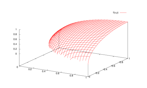
Figure 1: Graph of a morcave operator $f:{\overline{\mathbb{R}}}^{2}\to{\overline{\mathbb{R}}}$.

An important cmcave operator for our applications is the operator $\wedge$ on ${\overline{\mathbb{R}}}^{n}$:

Lemma 11

The operator $\vee$ on ${\overline{\mathbb{R}}}^{n}$ is monotone and convex, but not order-concave. The operator $\wedge$ on ${\overline{\mathbb{R}}}^{n}$ is cmcave, but not order-convex. ∎

Next, we extend the definition of affine functions from $\mathbb{R}^{n}\to\mathbb{R}^{m}$ to a definition of affine functions from ${\overline{\mathbb{R}}}^{n}\to{\overline{\mathbb{R}}}^{m}$.

Definition 3 (Affine Functions)

A function $f:\mathbb{R}^{n}\to\mathbb{R}^{m}$ is called affine if and only if there exist some $A\in\mathbb{R}^{m\times n}$ and some $b\in\mathbb{R}^{m}$ such that $f(x)=Ax+b$ for all $x\in\mathbb{R}^{n}$. A function $f:{\overline{\mathbb{R}}}^{n}\to{\overline{\mathbb{R}}}^{m}$ is called affine if and only if there exist some $A\in\mathbb{R}^{m\times n}$ and some $b\in{\overline{\mathbb{R}}}^{m}$ such that $f(x)=Ax+b$ for all $x\in{\overline{\mathbb{R}}}^{n}$. ∎

In the above definition and throughout this article, we use the convention that ${{-}\infty}+\infty={{-}\infty}$. Observe that an affine function $f$ with $f(x)=Ax+b$ is monotone, whenever all entries of the matrix $A$ are non-negative.

Lemma 12

Every affine function $f:\mathbb{R}^{n}\to\mathbb{R}^{m}$ is concave and convex. Every monotone and affine function $f:{\overline{\mathbb{R}}}^{n}\to{\overline{\mathbb{R}}}^{m}$ is cmcave. ∎

In contrast to the class of monotone and order-concave operators on $\mathbb{R}$, the class of morcave operators on ${\overline{\mathbb{R}}}$ is not closed under functional composition, as the following example shows:

Example 9

We consider the functions $f:{\overline{\mathbb{R}}}\to{\overline{\mathbb{R}}}$ and $g:{\overline{\mathbb{R}}}\to{\overline{\mathbb{R}}}$ defined by

$$f(x) :=\begin{cases}0&\text{if }x={{-}\infty}\\ 1&\text{if }x>{{-}\infty}\end{cases} g(x) :=\begin{cases}{{-}\infty}&\text{if }x<0\\ 0&\text{if }x\geq 0\end{cases} \text{for all }x\in{\overline{\mathbb{R}}}.$$ (12)

The functions $f$ and $g$ are both morcave — even cmcave. However, observe that

$$(f\circ g)(x)=f(g(x)) :=\begin{cases}0&\text{if }x<0\\ 1&\text{if }x\geq 0\end{cases} \text{for all }x\in{\overline{\mathbb{R}}}.$$ (13)

Then, $f\circ g$ is monotone, but not order-concave. ∎

As we will see, the composition $f\circ g$ of two morcave operators $f$ and $g$ is again morcave, if $f$ is additionally strict in the following sense: a function $f:{\overline{\mathbb{R}}}^{n}\to{\overline{\mathbb{R}}}$ is called strict if and only if $f(x)={{-}\infty}$ for all $x\in{\overline{\mathbb{R}}}^{n}$ with $x_{k\cdot}={{-}\infty}$ for some $k\in\{1,\ldots,n\}$.

Lemma 13

Let $f:{\overline{\mathbb{R}}}^{m}\to{\overline{\mathbb{R}}}$ and $g:{\overline{\mathbb{R}}}^{n}\to{\overline{\mathbb{R}}}^{m}$ be morcave. Assume additionally that $f$ is strict. Then $f\circ g$ is morcave.

Proof.

Since $f$ and $g$ are monotone, $f\circ g$ is also monotone. In order to show that $f\circ g$ is order-concave, let $I:\{1,\ldots,n\}\to\{{{-}\infty},\mathsf{id},\infty\}$ and $h:=(f\circ g)^{(I)}$.

1. The set $\operatorname{\mathsf{fdom}}(h)$ is order-convex by Lemma 9, since $h$ is monotone.

2. Let $x,y\in\operatorname{\mathsf{fdom}}(h)$ with $x\leq y$, $\lambda\in[0,1]$, and $z:=\lambda x+(1-\lambda)y$. Moreover, let $x^{\prime}:=g^{(I)}(x)$, $y^{\prime}:=g^{(I)}(y)$, and $z^{\prime}:=g^{(I)}(z)$. The strictness of $f$ implies that $z^{\prime}\rhd({{-}\infty},\ldots,{{-}\infty})$. Since $g^{(I)}$ is monotone, we get $x^{\prime}\leq y^{\prime}$. We define $I^{\prime}:\{1,\ldots,m\}\to\{{{-}\infty},\mathsf{id},\infty\}$ by

   $$I^{\prime}(k) =\begin{cases}\mathsf{id}&\text{if }z^{\prime}_{k\cdot}\in\mathbb{R}\\ \mathsf{\infty}&\text{if }z^{\prime}_{k\cdot}=\infty\end{cases} \text{for all }k\in\{1,\ldots,m\}.$$

   We get:

   $$h(z) =f(g^{(I)}(z))$$

   $$=f^{(I^{\prime})}(g^{(I)}(z))$$

   $$\geq f^{(I^{\prime})}(\lambda g^{(I)}(x)+(1-\lambda)g^{(I)}(y))$$

   (Monotonicity, Order-Concavity)

   $$=f^{(I^{\prime})}(\lambda x^{\prime}+(1-\lambda)y^{\prime})$$

   $$\geq\lambda f^{(I^{\prime})}(x^{\prime})+(1-\lambda)f^{(I^{\prime})}(y^{\prime})$$ (Order-Concavity)

   $$=\lambda f^{(I^{\prime})}(g^{(I)}(x))+(1-\lambda)f^{(I^{\prime})}(g^{(I)}(y))$$

   $$\geq\lambda f(g^{(I)}(x))+(1-\lambda)f(g^{(I)}(y)) f\leq f^{(I^{\prime})}$$ ()

   $$=\lambda h(x)+(1-\lambda)h(y)$$

   Hence, $h|_{\operatorname{\mathsf{fdom}}(h)}$ is order-concave.

3. Now, assume that $\operatorname{\mathsf{fdom}}(h)\neq\emptyset$. That is, there exists some $y\in\mathbb{R}^{n}$ with $h(y)=f(g^{(I)}(y))\in\mathbb{R}$. Since $f$ is strict, we get $y^{\prime}:=g^{(I)}(y)\rhd({{-}\infty},\ldots,{{-}\infty})$. Let $I^{\prime}:\{1,\ldots,m\}\to\{{{-}\infty},\mathsf{id},\infty\}$ be defined by

   $$I^{\prime}(k) =\begin{cases}\mathsf{id}&\text{if }y^{\prime}_{k\cdot}\in\mathbb{R}\\ \mathsf{\infty}&\text{if }y^{\prime}_{k\cdot}=\infty\end{cases} \text{for all }k\in\{1,\ldots,m\}.$$

   Since $g$ is order-concave, we get $g^{(I)}_{k\cdot}(x)<\infty$ for all $x\in\mathbb{R}^{n}$ and all $k\in\{1,\ldots,m\}$ with $y^{\prime}_{k\cdot}\in\mathbb{R}$. Since $f$ is order-concave, we get $f^{(I^{\prime})}(x)<\infty$ for all $x\in\mathbb{R}^{n}$. Thus, by monotonicity, we get $f^{(I^{\prime})}\circ g^{(I)}(x)=f^{(I^{\prime})}(g^{(I)}(x))<\infty$ for all $x\in\mathbb{R}^{n}$. Since we have $h=(f\circ g)^{(I)}\leq f^{(I^{\prime})}\circ g^{(I)}$ by construction, we get $h(x)<\infty$ for all $x\in\mathbb{R}^{n}$. ∎

∎

4 Solving Systems of $\vee$-morcave Equations

In this section, we present our $\vee$-strategy improvement algorithm for computing least solutions of systems of $\vee$-morcave equations and prove its correctness.

4.1 Systems of $\vee$-morcave Equations

Assume that a fixed finite set ${\bf X}$ of variables and a complete linearly ordered set $\mathbb{D}$ is given. Assume that $\mathbb{D}$ is partially ordered by $\leq$. We consider equations of the form ${\bf x}=e$ over $\mathbb{D}$, where ${\bf x}\in{\bf X}$ is a variable and $e$ is an expression over $\mathbb{D}$. A system ${\mathcal{E}}$ of (fixpoint-)equations over $\mathbb{D}$ is a finite set $\{{\bf x}_{1}=e_{1},\ldots,{\bf x}_{n}=e_{n}\}$ of equations, where ${\bf x}_{1},\ldots,{\bf x}_{n}$ are pairwise distinct variables. We denote the set $\{{\bf x}_{1},\allowbreak\ldots,\allowbreak{\bf x}_{n}\}$ of variables occurring in ${\mathcal{E}}$ by ${\bf X}_{\mathcal{E}}$. We drop the subscript, whenever it is clear from the context.

For a variable assignment $\rho:{\bf X}\to\mathbb{D}$, an expression $e$ is mapped to a value $\llbracket e\rrbracket\rho$ by setting $\llbracket{\bf x}\rrbracket\rho:=\rho({\bf x})$, and $\llbracket f(e_{1},\ldots,e_{k})\rrbracket\rho:=f(\llbracket e_{1}\rrbracket\rho,\ldots,\llbracket e_{k}\rrbracket\rho)$, where ${\bf x}\in{\bf X}$, $f$ is a $k$-ary operator ($k=0$ is possible; then $f$ is a constant), for instance $+$, and $e_{1},\ldots,e_{k}$ are expressions. For every system ${\mathcal{E}}$ of equations, we define the unary operator $\llbracket{\mathcal{E}}\rrbracket$ on ${\bf X}\to\mathbb{D}$ by setting $(\llbracket{\mathcal{E}}\rrbracket\rho)({\bf x}):=\llbracket e\rrbracket\rho$ for all equations ${\bf x}=e$ from ${\mathcal{E}}$ and all $\rho:{\bf X}\to\mathbb{D}$. A solution is a fixpoint of $\llbracket{\mathcal{E}}\rrbracket$, i.e., it is a variable assignment $\rho$ such that $\rho=\llbracket{\mathcal{E}}\rrbracket\rho$. We denote the set of all solutions of ${\mathcal{E}}$ by $\mathbf{Sol}({\mathcal{E}})$.

The set ${\bf X}\to\mathbb{D}$ of all variable assignments is a complete lattice. For $\rho,\rho^{\prime}:{\bf X}\to\mathbb{D}$, we write $\rho\lhd\rho^{\prime}$ (resp. $\rho\rhd\rho^{\prime}$) if and only if $\rho({\bf x})<\rho^{\prime}({\bf x})$ (resp. $\rho({\bf x})>\rho^{\prime}({\bf x})$) for all ${\bf x}\in{\bf X}$. For $d\in\mathbb{D}$, $\underline{d}$ denotes the variable assignment $\{{\bf x}\mapsto d\mid{\bf x}\in{\bf X}\}$. A variable assignment $\rho$ with $\underline{\bot}\lhd\rho\lhd\underline{\top}$ is called finite. A pre-solution (resp. post-solution) is a variable assignment $\rho$ such that $\rho\leq\llbracket{\mathcal{E}}\rrbracket\rho$ (resp. $\rho\geq\llbracket{\mathcal{E}}\rrbracket\rho$) holds. The set of pre-solutions (resp. the set of post-solutions) is denoted by $\mathbf{PreSol}({\mathcal{E}})$ (resp. $\mathbf{PostSol}({\mathcal{E}})$). The least solution (resp. the greatest solution) of a system ${\mathcal{E}}$ of equations is denoted by $\mu\llbracket{\mathcal{E}}\rrbracket$ (resp. $\nu\llbracket{\mathcal{E}}\rrbracket$), provided that it exists. For a pre-solution $\rho$ (resp. for a post-solution $\rho$), $\mu_{\geq\rho}\llbracket{\mathcal{E}}\rrbracket$ (resp. $\nu_{\leq\rho}\llbracket{\mathcal{E}}\rrbracket$) denotes the least solution that is greater than or equal to $\rho$ (resp. the greatest solution that is less than or equal to $\rho$).

An expression $e$ (resp. an (fixpoint-)equation ${\bf x}=e$ is called monotone if and only if $\llbracket e\rrbracket$ is monotone. In our setting, the fixpoint theorem of Knaster/Tarski can be stated as follows: every system ${\mathcal{E}}$ of monotone fixpoint equations over a complete lattice has a least solution $\mu\llbracket{\mathcal{E}}\rrbracket$ and a greatest solution $\nu\llbracket{\mathcal{E}}\rrbracket$. Furthermore, we have $\mu\llbracket{\mathcal{E}}\rrbracket=\bigwedge\mathbf{PostSol}({\mathcal{E}})$ and $\nu\llbracket{\mathcal{E}}\rrbracket=\bigvee\mathbf{PreSol}({\mathcal{E}})$.

Definition 4 ($\vee$-morcave Equations)

An expression $e$ (resp. fixpoint equation ${\bf x}=e$) over ${\overline{\mathbb{R}}}$ is called morcave (resp. cmorcave, resp. mcave, resp. cmcave) if and only if $\llbracket e\rrbracket$ is morcave (resp. cmorcave, resp. mcave, resp. cmcave). An expression $e$ (resp. fixpoint equation ${\bf x}=e$) over ${\overline{\mathbb{R}}}$ is called $\vee$-morcave (resp. $\vee$-cmorcave, resp. mcave, resp. cmcave) if and only if $e=e_{1}\vee\cdots\vee e_{k}$, where $e_{1},\ldots,e_{k}$ are morcave (resp. cmorcave, resp. mcave, resp. cmcave). ∎

Example 10

The square root operator $\sqrt{\cdot}:{\overline{\mathbb{R}}}\to{\overline{\mathbb{R}}}$ (defined by $\sqrt{x}:=\sup\;\{y\in\mathbb{R}\mid y^{2}\leq x\}$ for all $x\in{\overline{\mathbb{R}}}$) is cmcave. The least solution of the system ${\mathcal{E}}=\{{\bf x}=\frac{1}{2}\vee\sqrt{\bf x}\}$ of $\vee$-cmcave equations is $\mu\llbracket{\mathcal{E}}\rrbracket=1$. ∎

Definition 5 ($\vee$-strategies)

A $\vee$-strategy $\sigma$ for a system ${\mathcal{E}}$ of equations is a function that maps every expression $e_{1}\vee\cdots\vee e_{k}$ occurring in ${\mathcal{E}}$ to one of the immediate sub-expressions $e_{j}$, $j\in\{1,\ldots,k\}$. We denote the set of all $\vee$-strategies for ${\mathcal{E}}$ by $\Sigma_{\mathcal{E}}$. We drop the subscript, whenever it is clear from the context. The application ${\mathcal{E}}(\sigma)$ of $\sigma$ to ${\mathcal{E}}$ is defined by ${\mathcal{E}}(\sigma):=\{{\bf x}=\sigma(e)\mid{\bf x}=e\in{\mathcal{E}}\}$.

Example 11

The two $\vee$-strategies $\sigma_{1},\sigma_{2}$ for the system ${\mathcal{E}}$ of $\vee$-cmcave equations defined in Example 10 lead to the systems ${\mathcal{E}}(\sigma_{1})=\{{\bf x}=\frac{1}{2}\}$ and ${\mathcal{E}}(\sigma_{2})=\{{\bf x}=\sqrt{\bf x}\}$ of cmcave equations. ∎

4.2 The Strategy Improvement Algorithm

We now present the $\vee$-strategy improvement algorithm in a general setting. That is, we consider arbitrary systems of monotone equations over arbitrary complete linearly ordered sets $\mathbb{D}$. The algorithm iterates over $\vee$-strategies. It maintains a current $\vee$-strategy $\sigma$ and a current approximate $\rho$ to the least solution. A so-called $\vee$-strategy improvement operator is used to determine a next, improved $\vee$-strategy $\sigma^{\prime}$. Whether or not a $\vee$-strategy $\sigma^{\prime}$ is an improvement of the current $\vee$-strategy $\sigma$ may depend on the current approximate $\rho$:

Definition 6 (Improvements)

Let ${\mathcal{E}}$ be a system of monotone equations over a complete linearly ordered set. Let $\sigma,\sigma^{\prime}\in\Sigma$ be $\vee$-strategies for ${\mathcal{E}}$ and $\rho$ be a pre-solution of ${\mathcal{E}}(\sigma)$. The $\vee$-strategy $\sigma^{\prime}$ is called an improvement of $\sigma$ w.r.t. $\rho$ if and only if the following conditions are fulfilled:

1. If $\rho\notin\mathbf{Sol}({\mathcal{E}})$, then $\llbracket{\mathcal{E}}(\sigma^{\prime})\rrbracket\rho>\rho$.

2. For all expressions $e=e_{1}\vee\cdots\vee e_{k}$ of ${\mathcal{E}}$ the following holds: If $\sigma^{\prime}(e)\neq\sigma(e)$, then $\llbracket\sigma^{\prime}(e)\rrbracket\rho>\llbracket\sigma(e)\rrbracket\rho$.

A function $P_{\vee}$ that assigns an improvement of $\sigma$ w.r.t. $\rho$ to every pair $(\sigma,\rho)$, where $\sigma$ is a $\vee$-strategy and $\rho$ is a pre-solution of ${\mathcal{E}}(\sigma)$, is called a $\vee$-strategy improvement operator. If it is impossible to improve $\sigma$ w.r.t. $\rho$, then we necessarily have $P_{\vee}(\sigma,\rho)=\sigma$. ∎

Example 12

Consider the system ${\mathcal{E}}=\{{\bf x}_{1}={\bf x}_{2}+1\wedge 0,{\bf x}_{2}=-1\vee\sqrt{\bf x}_{1}\}$ of $\vee$-cmcave equations. Let $\sigma_{1}$ and $\sigma_{2}$ be the $\vee$-strategies for ${\mathcal{E}}$ such that

$${\mathcal{E}}(\sigma_{1}) =\{{\bf x}_{1}={\bf x}_{2}+1\wedge 0,{\bf x}_{2}=-1\},\text{ and}$$

$${\mathcal{E}}(\sigma_{2}) =\{{\bf x}_{1}={\bf x}_{2}+1\wedge 0,{\bf x}_{2}=\sqrt{\bf x}_{1}\}.$$

The variable assignment $\rho:=\{{\bf x}_{1}\mapsto 0,{\bf x}_{2}\mapsto-1\}$ is a solution and thus also a pre-solution of ${\mathcal{E}}(\sigma_{1})$. The $\vee$-strategy $\sigma_{2}$ is an improvement of the $\vee$-strategy $\sigma_{1}$ w.r.t. $\rho$. ∎

We can now formulate the $\vee$-strategy improvement algorithm for computing least solutions of systems of monotone equations over complete linearly ordered sets. This algorithm is parameterized with a $\vee$-strategy improvement operator $P_{\vee}$. The input is a system ${\mathcal{E}}$ of monotone equations over a complete linearly ordered set, a $\vee$-strategy $\sigma_{\mathrm{init}}$ for ${\mathcal{E}}$, and a pre-solution $\rho_{\mathrm{init}}$ of ${\mathcal{E}}(\sigma_{\mathrm{init}})$. In order to compute the least and not just some solution, we additionally require that $\rho_{\mathrm{init}}\leq\mu\llbracket{\mathcal{E}}\rrbracket$ holds:

$\\ \begin{array}[]{@{}l@{\text{:}\,}l@{}}\text{Parameter}&\text{A $\vee$-strategy improvement operator $P_{\vee}$}\\[2.84526pt] \text{Input}&\left\{\begin{array}[]{@{}l@{}}\text{\!\!-A system ${\mathcal{E}}$ of monotone equations over a complete linearly ordered set }\\ \text{\!\!-A $\vee$-strategy $\sigma_{\mathrm{init}}$ for ${\mathcal{E}}$}\\ \text{\!\!-A pre-solution $\rho_{\mathrm{init}}$ of ${\mathcal{E}}(\sigma_{\mathrm{init}})$ with $\rho_{\mathrm{init}}\leq\mu\llbracket{\mathcal{E}}\rrbracket$}\\ \end{array}\right.\\[14.22636pt] \text{Output}&\text{The least solution $\mu\llbracket{\mathcal{E}}\rrbracket$ of ${\mathcal{E}}$}\end{array}\\ \sigma\leftarrow\sigma_{\mathrm{init}};\\ \rho\leftarrow\rho_{\mathrm{init}};\\ \\ \mbox{while }(\rho\notin\mathbf{Sol}({\mathcal{E}}))\;\{\\ \hskip 14.22636pt\sigma\leftarrow P_{\vee}(\sigma,\rho);\\ \hskip 14.22636pt\rho\leftarrow\mu_{\geq\rho}\llbracket{\mathcal{E}}(\sigma)\rrbracket;\\ \}\\ \\ \mbox{return }\rho;\\$

Algorithm 1 The $\vee$-Strategy Improvement Algorithm

Example 13

We consider the system

$$\textstyle{\mathcal{E}}=\left\{{\bf x}={{-}\infty}\vee\frac{1}{2}\vee\sqrt{\bf x}\vee\frac{7}{8}+\sqrt{{\bf x}-\frac{47}{64}}\right\}$$ (14)

of $\vee$-cmorcave equations. We start with the $\vee$-strategy $\sigma_{0}$ that leads to the system

$${\mathcal{E}}(\sigma_{0})=\{{\bf x}={{-}\infty}\}$$ (15)

of cmorcave equations. Then $\rho_{0}:=\underline{{{-}\infty}}$ is a feasible solution of ${\mathcal{E}}(\sigma_{0})$. Since $\rho_{0}\notin\mathbf{Sol}({\mathcal{E}})$, we improve $\sigma_{0}$ w.r.t. $\rho_{0}$ to the $\vee$-strategy $\sigma_{1}$ that gives us

$${\mathcal{E}}(\sigma_{1})=\left\{{\bf x}=\frac{1}{2}\right\}.$$ (16)

Then, $\rho_{1}:=\mu_{\geq\rho_{0}}\llbracket\sigma_{1}\rrbracket=\{{\bf x}\mapsto\frac{1}{2}\}$. Since $\sqrt{\frac{1}{2}}>\frac{1}{2}$ and $\frac{7}{8}+\sqrt{\frac{1}{2}-\frac{47}{64}}<\frac{1}{2}$ hold, we improve the strategy $\sigma_{1}$ w.r.t. $\rho_{1}$ to the $\vee$-strategy $\sigma_{2}$ with

$${\mathcal{E}}(\sigma_{2})=\{{\bf x}=\sqrt{\bf x}\}.$$

We get $\rho_{2}:=\mu_{\geq\rho_{1}}\llbracket\sigma_{2}\rrbracket=\{{\bf x}\mapsto 1\}$. Since $\frac{7}{8}+\sqrt{1-\frac{47}{64}}>\frac{7}{8}+\sqrt{1-\frac{60}{64}}=\frac{9}{8}>1$, we get $\sigma_{3}=\{{\bf x}=\frac{7}{8}+\sqrt{{\bf x}-\frac{47}{64}}\}$. Finally we get $\rho_{3}:=\mu_{\geq\rho_{2}}\llbracket\sigma_{3}\rrbracket=\{{\bf x}\mapsto 2\}$. The algorithm terminates, because $\rho_{3}$ solves ${\mathcal{E}}$. Therefore, $\rho_{3}=\mu\llbracket{\mathcal{E}}\rrbracket$. ∎

In the following lemma, we collect basic properties that can be proven by induction straightforwardly:

Lemma 14

Let ${\mathcal{E}}$ be a system of monotone equations over a complete linearly ordered set. For all $i\in\mathbb{N}$, let $\rho_{i}$ be the value of the program variable $\rho$ and $\sigma_{i}$ be the value of the program variable $\sigma$ in the $\vee$-strategy improvement algorithm (Algorithm 1) after the $i$-th evaluation of the loop-body. The following statements hold for all $i\in\mathbb{N}$:

1. $\rho_{i}\leq\mu\llbracket{\mathcal{E}}\rrbracket$.

2. $\rho_{i}\in\mathbf{PreSol}({\mathcal{E}}(\sigma_{i+1}))$.

3. If $\rho_{i}<\mu\llbracket{\mathcal{E}}\rrbracket$, then $\rho_{i+1}>\rho_{i}$.

4. If $\rho_{i}=\mu\llbracket{\mathcal{E}}\rrbracket$, then $\rho_{i+1}=\rho_{i}$.

If the execution of the $\vee$-strategy improvement algorithm terminates, then the least solution $\mu\llbracket{\mathcal{E}}\rrbracket$ of ${\mathcal{E}}$ is computed. ∎

In the following, we apply our algorithm to solve systems of $\vee$-morcave equations. In the next subsection, we show that our algorithm terminates in this case. More precisely, it returns the least solution at the latest after considering every $\vee$-strategy at most $\left|{\bf X}\right|$ times. We additionally provide an important characterization of $\mu_{\geq\rho}\llbracket{\mathcal{E}}(\sigma)\rrbracket$ which allows us to compute it using convex optimization techniques. Here, $\sigma$ are the $\vee$-strategies and $\rho$ are the pre-solutions $\rho$ of ${\mathcal{E}}(\sigma)$ that can be encountered during the execution of the algorithm.

4.3 Feasibility

In this subsection, we extend the notion of feasibility as defined in Definition 1. We then show that feasibility is preserved during the execution of the $\vee$-strategy improvement algorithm. In the next subsection, we finally make use of the feasibility.

We denote by ${\mathcal{E}}[x_{1}/{\bf X}_{1},\ldots,x_{n}/{\bf X}_{n}]$ the equation system that is obtained from the equation system ${\mathcal{E}}$ by simultaneously replacing, for all $i\in\{1,\ldots,n\}$, every occurrence of a variable from the set ${\bf X}_{i}$ in the right-hand sides of ${\mathcal{E}}$ by the value $x_{i}$.

Definition 7 (Feasibility)

Let ${\mathcal{E}}$ be a system of morcave equations. A finite solution $\rho$ of ${\mathcal{E}}$ is called (${\mathcal{E}}$-)feasible if and only if $\rho$ is a feasible fixpoint of $\llbracket{\mathcal{E}}\rrbracket$. A pre-solution $\rho$ of ${\mathcal{E}}$ with $\llbracket{\mathcal{E}}\rrbracket\rho\rhd\underline{{{-}\infty}}$ is called (${\mathcal{E}}$-)feasible if and only if $\rho^{\prime}|_{{\bf X}^{\prime}}$ is a feasible finite solution of ${\mathcal{E}}^{\prime}:=\{{\bf x}=e\in{\mathcal{E}}\mid{\bf x}\in{\bf X}^{\prime}\}[\infty/({\bf X}\setminus{\bf X}^{\prime})]$, where $\rho^{\prime}:=\mu_{\geq\rho}\llbracket{\mathcal{E}}\rrbracket$ and ${\bf X}^{\prime}:=\{{\bf x}\in{\bf X}\mid\rho^{\prime}({\bf x})<\infty\}$. A pre-solution $\rho$ of ${\mathcal{E}}$ is called feasible if and only if $e={{-}\infty}$ for all ${\bf x}=e\in{\mathcal{E}}$ with $\llbracket e\rrbracket\rho={{-}\infty}$, and $\rho|_{{\bf X}^{\prime}}$ is a feasible pre-solution of ${\mathcal{E}}^{\prime}:=\{{\bf x}=e\in{\mathcal{E}}\mid{\bf x}\in{\bf X}^{\prime}\}[{{-}\infty}/({\bf X}\setminus{\bf X}^{\prime})]$, where ${\bf X}^{\prime}:=\{{\bf x}\mid{\bf x}=e\in{\mathcal{E}},\llbracket e\rrbracket\rho>{{-}\infty}\}$. ∎

Example 14

We consider the system ${\mathcal{E}}=\{{\bf x}=\sqrt{\bf x}\}$ of mcave equations. For all $x\in{\overline{\mathbb{R}}}$, let $\underline{x}:=\{{\bf x}\mapsto x\}$. From Example 1, we know that the solution $\underline{0}$ is not feasible, whereas the solution $\underline{1}$ is feasible. Thus, $\underline{x}$ is a feasible pre-solution for all $x\in(0,1]$. Note that $\underline{1}$ is the only feasible finite solution of ${\mathcal{E}}$ and thus, by Lemma 8, the greatest finite pre-solution of ${\mathcal{E}}$. ∎

Example 15

Let us consider the system ${\mathcal{E}}=\{{\bf x}_{1}={\bf x}_{2}+1\wedge 0,{\bf x}_{2}=\sqrt{\bf x}_{1}\}$ of mcave equations. From Example 6 it follows that $\rho:=\{{\bf x}_{1}\mapsto 0,{\bf x}_{2}\mapsto 0\}$ is a feasible finite fixpoint of $\llbracket{\mathcal{E}}\rrbracket$. Thus, $\{{\bf x}_{1}\mapsto 0,{\bf x}_{2}\mapsto x\}$ is a feasible pre-solution for all $x\in[-1,0]$. The solution $\{{\bf x}_{1}\mapsto{{-}\infty},{\bf x}_{2}\mapsto{{-}\infty}\}$ is not feasible, since the right-hand sides evaluate to ${{-}\infty}$, although they are not ${{-}\infty}$. ∎

The following two lemma imply that our $\vee$-strategy improvement algorithm stays in the feasible area, whenever it is started in the feasible area.

Lemma 15

Let ${\mathcal{E}}$ be a system of morcave equations and $\rho$ be a feasible pre-solution of ${\mathcal{E}}$. Every pre-solution $\rho^{\prime}$ of ${\mathcal{E}}$ with $\rho\leq\rho^{\prime}\leq\mu_{\geq\rho}\llbracket{\mathcal{E}}\rrbracket$ is feasible.

Proof.

The statement is an immediate consequence of the definition. ∎∎

Lemma 16

Let ${\mathcal{E}}$ be a system of $\vee$-morcave equations, $\sigma$ be a $\vee$-strategy for ${\mathcal{E}}$, $\rho$ be a feasible solution of ${\mathcal{E}}(\sigma)$, and $\sigma^{\prime}$ be an improvement of $\sigma$ w.r.t. $\rho$. Then $\rho$ is a feasible pre-solution of ${\mathcal{E}}(\sigma^{\prime})$.

Proof.

Let $\rho^{*}:=\mu_{\geq\rho}\llbracket{\mathcal{E}}(\sigma^{\prime})\rrbracket$. We w.l.o.g. assume that $\underline{{{-}\infty}}\lhd\rho^{*}\lhd\underline{\infty}$. Hence, $\rho\lhd\underline{\infty}$. Let

$${\bf X}^{\mathsf{old}} :=\{{\bf x}\in{\bf X}\mid\rho({\bf x})>{{-}\infty}\},\text{and }$$

$${\mathcal{E}}^{\mathsf{old}} :=\{{\bf x}=e\in{\mathcal{E}}(\sigma)\mid{\bf x}\in{\bf X}^{\mathsf{old}}\}[{{-}\infty}/({\bf X}\setminus{\bf X}^{\mathsf{old}})].$$

Hence, $\rho|_{{\bf X}^{\mathsf{old}}}$ is a feasible finite solution of ${\mathcal{E}}^{\mathsf{old}}$, i.e., a feasible finite fixpoint of $\llbracket{\mathcal{E}}^{\mathsf{old}}\rrbracket$. Therefore, there exist ${\bf X}_{1}\operatorname{{\dot{\cup}}}\cdots\operatorname{{\dot{\cup}}}{\bf X}_{k}={\bf X}^{\mathsf{old}}$ with

$${\bf X}_{1}\stackrel{{\scriptstyle\llbracket{\mathcal{E}}^{\mathsf{old}}\rrbracket,\rho|_{{\bf X}^{\mathsf{old}}}}}{{\rightarrow}}\cdots\stackrel{{\scriptstyle\llbracket{\mathcal{E}}^{\mathsf{old}}\rrbracket,\rho|_{{\bf X}^{\mathsf{old}}}}}{{\rightarrow}}{\bf X}_{k}$$ (17)

such that, for each $j\in\{1,\ldots,k\}$, there exists some pre-fixpoint $\rho^{\prime}$ of $\llbracket{\mathcal{E}}^{\mathsf{old}}\rrbracket\leftarrow\rho|_{{\bf X}^{\mathsf{old}}\setminus{\bf X}_{j}}$ with $\rho^{\prime}\lhd\rho|_{{\bf X}_{j}}$ such that $\mu_{\geq\rho^{\prime}}(\llbracket{\mathcal{E}}^{\mathsf{old}}\rrbracket\leftarrow\rho|_{{\bf X}^{\mathsf{old}}\setminus{\bf X}_{j}})=\rho|_{{\bf X}_{j}}$.

Let ${\bf X}^{\mathsf{imp}}:=\{{\bf x}\in{\bf X}\mid\rho^{*}({\bf x})>\rho({\bf x})\}$, ${\bf X}_{j}^{\prime}:={\bf X}_{j}\setminus{\bf X}^{\mathsf{imp}}$ for all $j\in\{1,\ldots,k\}$, and ${\bf X}_{k+1}^{\prime}:={\bf X}^{\mathsf{imp}}$. Obviously, we have ${\bf X}_{1}^{\prime}\operatorname{{\dot{\cup}}}\cdots\operatorname{{\dot{\cup}}}{\bf X}_{k+1}^{\prime}={\bf X}$. It remains to show that the following properties are fulfilled:

1. ${\bf X}_{1}^{\prime}\stackrel{{\scriptstyle\llbracket{\mathcal{E}}(\sigma^{\prime})\rrbracket,\rho^{*}}}{{\rightarrow}}\cdots\stackrel{{\scriptstyle\llbracket{\mathcal{E}}(\sigma^{\prime})\rrbracket,\rho^{*}}}{{\rightarrow}}{\bf X}_{k+1}^{\prime}$

2. For each $j\in\{1,\ldots,k+1\}$, there exists some pre-fixpoint $\rho^{\prime}$ with $\rho^{\prime}\lhd\rho^{*}|_{{\bf X}_{j}^{\prime}}$ such that $\mu_{\geq\rho^{\prime}}(\llbracket{\mathcal{E}}(\sigma^{\prime})\rrbracket\leftarrow\rho^{*}|_{{\bf X}\setminus{\bf X}_{j}^{\prime}})=\rho^{*}|_{{\bf X}_{j}^{\prime}}$.

In order to prove statement 1, let $j\in\{1,\ldots,k\}$. We have to show that

$${\bf X}_{1}^{\prime}\operatorname{{\dot{\cup}}}\cdots\operatorname{{\dot{\cup}}}{\bf X}_{j}^{\prime}\stackrel{{\scriptstyle\llbracket{\mathcal{E}}(\sigma^{\prime})\rrbracket,\rho^{*}}}{{\rightarrow}}{\bf X}_{j+1}^{\prime}\operatorname{{\dot{\cup}}}\cdots\operatorname{{\dot{\cup}}}{\bf X}_{k+1}^{\prime}.$$

Since ${\bf X}_{1}\operatorname{{\dot{\cup}}}\cdots\operatorname{{\dot{\cup}}}{\bf X}_{j}\stackrel{{\scriptstyle\llbracket{\mathcal{E}}^{\mathsf{old}}\rrbracket,\rho|_{{\bf X}^{\mathsf{old}}}}}{{\rightarrow}}{\bf X}_{j+1}\operatorname{{\dot{\cup}}}\cdots\operatorname{{\dot{\cup}}}{\bf X}_{k}$, there exists some variable assignment $\rho^{\prime}:{\bf X}_{j+1}\operatorname{{\dot{\cup}}}\cdots\operatorname{{\dot{\cup}}}{\bf X}_{k}\to\mathbb{R}$ with $\rho^{\prime}\lhd\rho|_{{\bf X}_{j+1}\operatorname{{\dot{\cup}}}\cdots\operatorname{{\dot{\cup}}}{\bf X}_{k}}$ such that

$$(\llbracket{\mathcal{E}}^{\mathsf{old}}\rrbracket(\rho|_{{\bf X}^{\mathsf{old}}}\oplus\rho^{\prime}))|_{{\bf X}_{1}\operatorname{{\dot{\cup}}}\cdots\operatorname{{\dot{\cup}}}{\bf X}_{j}}=(\llbracket{\mathcal{E}}^{\mathsf{old}}\rrbracket(\rho|_{{\bf X}^{\mathsf{old}}}))|_{{\bf X}_{1}\operatorname{{\dot{\cup}}}\cdots\operatorname{{\dot{\cup}}}{\bf X}_{j}}.$$ (18)

We define $\rho^{\prime\prime}:{\bf X}_{j+1}^{\prime}\operatorname{{\dot{\cup}}}\cdots\operatorname{{\dot{\cup}}}{\bf X}_{k+1}^{\prime}\to\mathbb{R}$ by

$$\rho^{\prime\prime}({\bf x}){=}\begin{cases}\rho^{\prime}({\bf x})&\text{if }{\bf x}\in{\bf X}_{j+1}^{\prime}\operatorname{{\dot{\cup}}}\cdots\operatorname{{\dot{\cup}}}{\bf X}_{k}^{\prime}\\ \rho({\bf x})&\text{if }{\bf x}\in{\bf X}_{k+1}^{\prime}\text{ and }{\bf x}\in{\bf X}^{\mathsf{old}}\\ \rho^{*}({\bf x})-1&\!\text{if }{\bf x}\in{\bf X}_{k+1}^{\prime}\text{ and }{\bf x}\notin{\bf X}^{\mathsf{old}}\\ \end{cases} \text{for all }{\bf x}\in{\bf X}_{j+1}^{\prime}\operatorname{{\dot{\cup}}}\cdots\operatorname{{\dot{\cup}}}{\bf X}_{k+1}^{\prime}.$$

By construction, we have $\rho^{\prime\prime}\lhd\rho^{*}|_{{\bf X}_{j+1}^{\prime}\operatorname{{\dot{\cup}}}\cdots\operatorname{{\dot{\cup}}}{\bf X}_{k+1}^{\prime}}$. Hence, we get

$$(\llbracket{\mathcal{E}}(\sigma^{\prime})\rrbracket(\rho^{*}))|_{{\bf X}_{1}^{\prime}\operatorname{{\dot{\cup}}}\cdots\operatorname{{\dot{\cup}}}{\bf X}_{j}^{\prime}} \geq(\llbracket{\mathcal{E}}(\sigma^{\prime})\rrbracket(\rho^{*}\oplus\rho^{\prime\prime}))|_{{\bf X}_{1}^{\prime}\operatorname{{\dot{\cup}}}\cdots\operatorname{{\dot{\cup}}}{\bf X}_{j}^{\prime}} \rho^{*}\geq\rho^{*}\oplus\rho^{\prime\prime}$$ ()

$$\geq(\llbracket{\mathcal{E}}^{\mathsf{old}}\rrbracket(\rho|_{{\bf X}^{\mathsf{old}}}\oplus\rho^{\prime}))|_{{\bf X}_{1}^{\prime}\operatorname{{\dot{\cup}}}\cdots\operatorname{{\dot{\cup}}}{\bf X}_{j}^{\prime}}$$

$$=(\llbracket{\mathcal{E}}^{\mathsf{old}}\rrbracket(\rho|_{{\bf X}^{\mathsf{old}}}))|_{{\bf X}_{1}^{\prime}\operatorname{{\dot{\cup}}}\cdots\operatorname{{\dot{\cup}}}{\bf X}_{j}^{\prime}}$$ (because of (18))

$$=(\llbracket{\mathcal{E}}^{\mathsf{old}}\rrbracket(\rho^{*}|_{{\bf X}^{\mathsf{old}}}))|_{{\bf X}_{1}^{\prime}\operatorname{{\dot{\cup}}}\cdots\operatorname{{\dot{\cup}}}{\bf X}_{j}^{\prime}}$$ (because of Lemma 7)

$$=(\llbracket{\mathcal{E}}(\sigma^{\prime})\rrbracket(\rho^{*}))|_{{\bf X}_{1}^{\prime}\operatorname{{\dot{\cup}}}\cdots\operatorname{{\dot{\cup}}}{\bf X}_{j}^{\prime}}.$$

Thus, $(\llbracket{\mathcal{E}}(\sigma^{\prime})\rrbracket(\rho^{*}\oplus\rho^{\prime\prime}))|_{{\bf X}_{1}^{\prime}\operatorname{{\dot{\cup}}}\cdots\operatorname{{\dot{\cup}}}{\bf X}_{j}^{\prime}}=(\llbracket{\mathcal{E}}(\sigma^{\prime})\rrbracket(\rho^{*}))|_{{\bf X}_{1}^{\prime}\operatorname{{\dot{\cup}}}\cdots\operatorname{{\dot{\cup}}}{\bf X}_{j}^{\prime}}$. This proves statement 1.

In order to prove statement 2, let $j\in\{1,\ldots,k+1\}$. We distinguish 2 cases. Firstly, assume that $j\leq k$. Since $\rho|_{{\bf X}^{\mathsf{old}}}$ is a feasible finite fixpoint of $\llbracket{\mathcal{E}}^{\mathsf{old}}\rrbracket$, there exists some pre-fixpoint $\rho^{\prime}$ with $\rho^{\prime}\lhd\rho|_{{\bf X}_{j}}=\rho^{*}|_{{\bf X}_{j}}$ such that $\mu_{\geq\rho^{\prime}}(\llbracket{\mathcal{E}}^{\mathsf{old}}\rrbracket\leftarrow\rho|_{{\bf X}^{\mathsf{old}}\setminus{\bf X}_{j}})=\rho|_{{\bf X}_{j}}=\rho^{*}|_{{\bf X}_{j}}$. Using monotonicity, we get $\mu_{\geq\rho^{\prime}}(\llbracket{\mathcal{E}}^{\mathsf{old}}\rrbracket\leftarrow\rho^{*}|_{{\bf X}^{\mathsf{old}}\setminus{\bf X}_{j}})\allowbreak=\rho|_{{\bf X}_{j}}=\rho^{*}|_{{\bf X}_{j}}$. Hence, $\rho^{\prime}|_{{\bf X}_{j}^{\prime}}:{\bf X}_{j}^{\prime}\to\mathbb{R}$, $\rho^{\prime}|_{{\bf X}_{j}^{\prime}}\lhd\rho|_{{\bf X}_{j}^{\prime}}=\rho^{*}|_{{\bf X}_{j}^{\prime}}$, and $\mu_{\geq\rho^{\prime}|_{{\bf X}_{j}^{\prime}}}(\llbracket{\mathcal{E}}^{\mathsf{old}}\rrbracket\allowbreak\leftarrow\rho^{*}|_{{\bf X}^{\mathsf{old}}\setminus{\bf X}_{j}^{\prime}})=\mu_{\geq\rho^{\prime}|_{{\bf X}_{j}^{\prime}}}(\llbracket{\mathcal{E}}(\sigma^{\prime})\rrbracket\leftarrow\rho^{*}|_{{\bf X}\setminus{\bf X}_{j}^{\prime}})=\rho^{*}|_{{\bf X}_{j}^{\prime}}$. This proves statement 2 for $j\leq k$. Now, assume that $j=k+1$. By definition of ${\bf X}_{k+1}^{\prime}$, $\rho|_{{\bf X}_{k+1}^{\prime}}\lhd\rho^{*}|_{{\bf X}_{k+1}^{\prime}}$. Moreover, we get immediately that $\rho|_{{\bf X}_{k+1}^{\prime}}$ is a pre-fixpoint of $\llbracket{\mathcal{E}}(\sigma^{\prime})\rrbracket\leftarrow\rho^{*}|_{{\bf X}\setminus{\bf X}_{k+1}^{\prime}}$ and $\mu_{\geq\rho|_{{\bf X}_{k+1}^{\prime}}}(\llbracket{\mathcal{E}}(\sigma^{\prime})\rrbracket\leftarrow\rho^{*}|_{{\bf X}\setminus{\bf X}_{k+1}^{\prime}})=\rho^{*}|_{{\bf X}_{k+1}^{\prime}}$. This proves statement 2. ∎∎

Example 16

We continue Example 12. Obviously, $\rho=\{{\bf x}_{1}\mapsto 0,{\bf x}_{2}\mapsto-1\}$ is a feasible solution of ${\mathcal{E}}(\sigma_{1})=\{{\bf x}_{1}={\bf x}_{2}+1\wedge 0,{\bf x}_{2}=-1\}$. The $\vee$-strategy $\sigma_{2}$ is an improvement of the $\vee$-strategy $\sigma_{1}$ w.r.t. $\rho$. By lemma 16, $\rho$ is also a feasible pre-solution of ${\mathcal{E}}(\sigma_{2})=\{{\bf x}_{1}={\bf x}_{2}+1\wedge 0,{\bf x}_{2}=\sqrt{\bf x}_{1}\}$. The fact that $\rho$ is a feasible pre-solution of ${\mathcal{E}}(\sigma_{2})$ is also shown in Example 15. ∎

The above two lemmas ensure that our $\vee$-strategy improvement algorithm stays in the feasible area, whenever it is started in the feasible area. In order to start in the feasible area, we in the following simply assume w.l.o.g. that each equation of ${\mathcal{E}}$ is of the form ${\bf x}={{-}\infty}\vee e$. We say that such a system of fixpoint equations is in standard form. Then, we start our $\vee$-strategy improvement algorithm with a $\vee$-strategy $\sigma_{\mathrm{init}}$ such that ${\mathcal{E}}(\sigma_{\mathrm{init}})=\{{\bf x}={{-}\infty}\mid{\bf x}\in{\bf X}\}$. In consequence, $\underline{{{-}\infty}}$ is a feasible solution of ${\mathcal{E}}(\sigma_{\mathrm{init}})$. We get:

Lemma 17

Let ${\mathcal{E}}$ be a system of $\vee$-morcave equations. For all $i\in\mathbb{N}$, let $\rho_{i}$ be the value of the program variable $\rho$ and $\sigma_{i}$ be the value of the program variable $\sigma$ in the $\vee$-strategy improvement algorithm (Algorithm 1) after the $i$-th evaluation of the loop-body. Then, $\rho_{i}$ is a feasible pre-solution of ${\mathcal{E}}(\sigma_{i+1})$ for all $i\in\mathbb{N}$. ∎

Example 17

We again consider the system ${\mathcal{E}}=\{{\bf x}_{1}={{-}\infty}\vee{\bf x}_{2}+1\wedge 0,\;{\bf x}_{2}={{-}\infty}\vee-1\vee\sqrt{\bf x}_{1}\}$ of $\vee$-morcave equations introduced in Example 12. A run of our $\vee$-strategy improvement algorithm gives us

$${\mathcal{E}}(\sigma_{0}) =\{{\bf x}_{1}={{-}\infty},\;{\bf x}_{2}={{-}\infty}\} \rho_{0} =\{{\bf x}_{1}\mapsto{{-}\infty},\;{\bf x}_{2}\mapsto{{-}\infty}\}$$

$${\mathcal{E}}(\sigma_{1}) =\{{\bf x}_{1}={{-}\infty},\;{\bf x}_{2}=-1\} \rho_{1} =\{{\bf x}_{1}\mapsto{{-}\infty},\;{\bf x}_{2}\mapsto-1\}$$

$${\mathcal{E}}(\sigma_{2}) =\{{\bf x}_{1}={\bf x}_{2}+1\wedge 0,\;{\bf x}_{2}=-1\} \rho_{2} =\{{\bf x}_{1}\mapsto 0,\;{\bf x}_{2}\mapsto-1\}$$

$${\mathcal{E}}(\sigma_{3}) =\{{\bf x}_{1}={\bf x}_{2}+1\wedge 0,\;{\bf x}_{2}=\sqrt{{\bf x}_{1}}\} \rho_{3} =\{{\bf x}_{1}\mapsto 0,\;{\bf x}_{2}\mapsto 0\}$$

By Lemma 17, $\rho_{i}$ is a feasible pre-solution of ${\mathcal{E}}(\sigma_{i+1})$ for all $i=\{0,1,2\}$. ∎

4.4 Evaluating $\vee$-Strategies / Solving Systems of Morcave Equations

It remains to develop a method for computing $\mu_{\geq\rho}\llbracket{\mathcal{E}}\rrbracket$ under the assumption that $\rho$ is a feasible pre-solution of the system ${\mathcal{E}}$ of morcave equations. This is an important step in our $\vee$-strategy improvement algorithm (Algorithm 1). Before doing this, we introduce the following notation for the sake of simplicity:

Definition 8

Let ${\mathcal{E}}$ be a system of morcave equations and $\rho$ a pre-solution of ${\mathcal{E}}$. Let

$${\bf X}^{{-}\infty}_{\rho} :=\{{\bf x}\mid{\bf x}=e\in{\mathcal{E}},\;\llbracket e\rrbracket\rho={{-}\infty}\}$$ (19)

$${\bf X}^{\infty}_{\rho} :=\{{\bf x}\mid{\bf x}=e\in{\mathcal{E}},\;\llbracket e\rrbracket\rho=\infty\}$$ (20)

$${\bf X}^{\prime}_{\rho} :={\bf X}\setminus({\bf X}^{{-}\infty}_{\rho}\cup{\bf X}^{\infty}_{\rho})=\{{\bf x}\mid{\bf x}=e\in{\mathcal{E}},\;\llbracket e\rrbracket\rho\in\mathbb{R}\}$$ (21)

$${\mathcal{E}}^{\prime}_{\rho} =\{{\bf x}=e\in{\mathcal{E}}\mid{\bf x}\in{\bf X}^{\prime}_{\rho}\}[{{-}\infty}/{\bf X}^{{-}\infty}_{\rho},\infty/{\bf X}^{\infty}_{\rho}]$$ (22)

The pre-solution $\mathsf{suppresol}_{\rho}\llbracket{\mathcal{E}}\rrbracket$ of ${\mathcal{E}}$ is defined by

$$\mathsf{suppresol}_{\rho}\llbracket{\mathcal{E}}\rrbracket({\bf x}) :=\begin{cases}{{-}\infty}&\text{if }{\bf x}\in{\bf X}^{{-}\infty}_{\rho}\\ \sup\;\{\hat{\rho}({\bf x})\mid\hat{\rho}:{\bf X}^{\prime}_{\rho}\to\mathbb{R},\;\hat{\rho}\leq\llbracket{\mathcal{E}}^{\prime}\rrbracket\hat{\rho}\}&\text{if }{\bf x}\in{\bf X}^{\prime}_{\rho}\\ \infty&\text{if }{\bf x}\in{\bf X}^{\infty}_{\rho}\end{cases}$$ (23)

for all ${\bf x}\in{\bf X}$. ∎

Remark 1

The variables assignment $\mathsf{suppresol}_{\rho}\llbracket{\mathcal{E}}\rrbracket$ is by construction a pre-solution of ${\mathcal{E}}$, but, as we will see in Example 18, not necessarily a solution of ${\mathcal{E}}$. ∎

Under some constraints, we can compute $\mathsf{suppresol}_{\rho}\llbracket{\mathcal{E}}\rrbracket$ by solving $\left|{\bf X}\right|$ convex optimisation problems of linear size. This can be done by general convex optimization methods. For further information on convex optimization, we refer, for instance, to Nemirovski [13].

Lemma 18

Let ${\mathcal{E}}$ be a system of mcave equations and $\rho$ a pre-solution of ${\mathcal{E}}$. Then, the pre-solution $\mathsf{suppresol}_{\rho}\llbracket{\mathcal{E}}\rrbracket$ of ${\mathcal{E}}$ can be computed by solving at most $\left|{\bf X}\right|$ convex optimization problems.

Proof.

Let ${\bf X}^{{-}\infty}_{\rho}$, ${\bf X}^{\infty}_{\rho}$, ${\bf X}^{\prime}_{\rho}$, and ${\mathcal{E}}^{\prime}_{\rho}$ be defined as in Definition 8. We have to compute $\mathsf{suppresol}_{\rho}\llbracket{\mathcal{E}}\rrbracket({\bf x})=\sup\;\{\hat{\rho}({\bf x})\mid\hat{\rho}:{\bf X}^{\prime}_{\rho}\to\mathbb{R},\;\hat{\rho}\leq\llbracket{\mathcal{E}}^{\prime}\rrbracket\hat{\rho}\}=\sup\;\{\hat{\rho}({\bf x})\mid\hat{\rho}:{\bf X}^{\prime}_{\rho}\to\mathbb{R},\;(\mathsf{id}-\llbracket{\mathcal{E}}^{\prime}\rrbracket)\hat{\rho}\leq 0\}$ for all ${\bf x}\in{\bf X}^{\prime}_{\rho}$. Here, $\mathsf{id}$ denotes the identity function. Therefore, since $\mathsf{id}$ is affine, $\llbracket{\mathcal{E}}^{\prime}\rrbracket$ is concave (considered as a function that maps values from ${\bf X}^{\prime}_{\rho}\to\mathbb{R}$ to values from ${\bf X}^{\prime}_{\rho}\to(\mathbb{R}\cup\{{{-}\infty}\}$), and thus $-\llbracket{\mathcal{E}}^{\prime}\rrbracket\hat{\rho}$ is convex (considered as a function that maps values from ${\bf X}^{\prime}_{\rho}\to\mathbb{R}$ to values from ${\bf X}^{\prime}_{\rho}\to(\mathbb{R}\cup\{\infty\}$), the mathematical optimization problem $\sup\;\{\hat{\rho}({\bf x})\mid\hat{\rho}:{\bf X}^{\prime}_{\rho}\to\mathbb{R},\;(\mathsf{id}-\llbracket{\mathcal{E}}^{\prime}\rrbracket)\hat{\rho}\leq 0\}$ is a convex optimization problem. ∎∎

We will use $\mathsf{suppresol}_{\rho}\llbracket{\mathcal{E}}\rrbracket$ iteratively to compute $\mu_{\geq\rho}\llbracket{\mathcal{E}}\rrbracket$ under the assumption that $\rho$ is a feasible pre-solution of the system ${\mathcal{E}}$ of morcave equations. As a first step in this direction, we prove the following lemma, which gives us at least a method for computing $\mu_{\geq\rho}\llbracket{\mathcal{E}}\rrbracket$ under the assumption that ${\mathcal{E}}$ is a system of cmorcaveequations.

Lemma 19

Let ${\mathcal{E}}$ be a system of morcave equations and $\rho$ a feasible pre-solution of ${\mathcal{E}}$. Let ${\bf X}^{{-}\infty}_{\rho}$, ${\bf X}^{\infty}_{\rho}$, and ${\bf X}^{\prime}_{\rho}$ be defined as in Definition 8 ((19) - (21)). Then:

$$\mu_{\geq\rho}\llbracket{\mathcal{E}}\rrbracket({\bf x}) =\mathsf{suppresol}_{\rho}\llbracket{\mathcal{E}}\rrbracket({\bf x})={{-}\infty} \text{for all }{\bf x}\in{\bf X}^{{-}\infty}_{\rho}$$ (24)

$$\mu_{\geq\rho}\llbracket{\mathcal{E}}\rrbracket({\bf x}) \geq\mathsf{suppresol}_{\rho}\llbracket{\mathcal{E}}\rrbracket({\bf x}) \text{for all }{\bf x}\in{\bf X}^{\prime}_{\rho}$$ (25)

$$\mu_{\geq\rho}\llbracket{\mathcal{E}}\rrbracket({\bf x}) =\mathsf{suppresol}_{\rho}\llbracket{\mathcal{E}}\rrbracket({\bf x})=\infty \text{for all }{\bf x}\in{\bf X}^{\infty}_{\rho}$$ (26)

If ${\mathcal{E}}$ is a system of cmorcave equations, then the inequality in (25) is in fact an equality, i.e., we have

$$\mu_{\geq\rho}\llbracket{\mathcal{E}}\rrbracket =\mathsf{suppresol}_{\rho}\llbracket{\mathcal{E}}\rrbracket.$$ (27)

Proof.

Let ${\mathcal{E}}^{\prime}_{\rho}$ be defined as in Definition 8 (22). We first prove (24) - (26). Let $x\in{\bf X}$. If ${\bf x}\in{\bf X}^{{-}\infty}_{\rho}\cup{\bf X}^{\infty}_{\rho}$, then the statement is obviously fulfilled, because $\rho$ is feasible and thus $e={{-}\infty}$ for all equations ${\bf x}=e$ from ${\mathcal{E}}$ with $\llbracket e\rrbracket\rho={{-}\infty}$. This gives us (24) and (26). Assume now that ${\bf x}\in{\bf X}^{\prime}_{\rho}$. Let $\rho^{\prime}:=\rho|_{{\bf X}^{\prime}_{\rho}}$ and $\rho^{*}:=\mu_{\geq\rho^{\prime}}\llbracket{\mathcal{E}}^{\prime}_{\rho}\rrbracket$. We have to show that

$$\rho^{*}({\bf x})\geq\sup\;\{\hat{\rho}({\bf x})\mid\hat{\rho}:{\bf X}^{\prime}_{\rho}\to\mathbb{R},\;\hat{\rho}\leq\llbracket{\mathcal{E}}^{\prime}_{\rho}\rrbracket\hat{\rho}\}.$$ (28)

If $\rho^{*}({\bf x})=\infty$, there is nothing to prove. Therefore, assume that $\rho^{*}({\bf x})<\infty$. Then $\rho^{*}({\bf x})\in\mathbb{R}$. Let ${\bf X}^{\prime\prime}_{\rho}:=\{{\bf x}^{\prime\prime}\in{\bf X}^{\prime}_{\rho}\mid\rho^{*}({\bf x}^{\prime\prime})<\infty\}$. Then, ${\bf X}^{\prime\prime}_{\rho}=\{{\bf x}^{\prime\prime}\in{\bf X}^{\prime}_{\rho}\mid\rho^{*}({\bf x}^{\prime\prime})\in\mathbb{R}\}$. Let ${\mathcal{E}}^{\prime\prime}_{\rho}:=\{{\bf x}^{\prime\prime}=e\in{\mathcal{E}}^{\prime}_{\rho}\mid{\bf x}^{\prime\prime}\in{\bf X}^{\prime\prime}_{\rho}\}[\infty/({\bf X}^{\prime}_{\rho}\setminus{\bf X}^{\prime\prime}_{\rho})]$, and $\rho^{\prime\prime}:=\rho|_{{\bf X}^{\prime\prime}_{\rho}}$. The pre-solution $\rho^{\prime\prime}$ of ${\mathcal{E}}^{\prime\prime}_{\rho}$ is feasible. Hence, $\rho^{*}|_{{\bf X}^{\prime\prime}_{\rho}}$ is a feasible finite pre-solution of ${\mathcal{E}}^{\prime\prime}_{\rho}$, i.e., a feasible finite fixpoint of $\llbracket{\mathcal{E}}^{\prime\prime}_{\rho}\rrbracket$. Therefore, we finally get (25) using Lemma 8.

Before we actually prove (27), we start with an easy observation. The sequence $(\llbracket{\mathcal{E}}^{\prime}_{\rho}\rrbracket^{k}\rho^{\prime})_{k\in\mathbb{N}}$ is increasing, because $\rho^{\prime}$ is a pre-solution of ${\mathcal{E}}^{\prime}_{\rho}$. Further $\llbracket{\mathcal{E}}^{\prime}_{\rho}\rrbracket^{k}\rho^{\prime}:{\bf X}^{\prime}_{\rho}\to\mathbb{R}$ and $\llbracket{\mathcal{E}}^{\prime}_{\rho}\rrbracket^{k}\rho^{\prime}\leq\llbracket{\mathcal{E}}^{\prime}_{\rho}\rrbracket(\llbracket{\mathcal{E}}^{\prime}_{\rho}\rrbracket^{k}\rho^{\prime})$ for all $k\in\mathbb{N}$. Hence, we get

$$\sup\;\{\hat{\rho}({\bf x})\mid\hat{\rho}:{\bf X}^{\prime}_{\rho}\to\mathbb{R},\;\hat{\rho}\leq\llbracket{\mathcal{E}}^{\prime}_{\rho}\rrbracket\hat{\rho}\}\geq\sup\;\{(\llbracket{\mathcal{E}}^{\prime}_{\rho}\rrbracket^{k}\rho^{\prime})({\bf x})\mid k\in\mathbb{N}\}$$ (29)

Now, assume that ${\mathcal{E}}$ is a system of cmorcave equations. In order to prove (27), it remains to show that $\rho^{*}({\bf x})\leq\sup\;\{\hat{\rho}({\bf x})\mid\hat{\rho}:{\bf X}^{\prime}_{\rho}\to\mathbb{R},\;\hat{\rho}\leq\llbracket{\mathcal{E}}^{\prime}_{\rho}\rrbracket\hat{\rho}\}$. Since $\llbracket{\mathcal{E}}^{\prime}_{\rho}\rrbracket$ is monotone and upward-chain-continuous on $\{\hat{\rho}:{\bf X}^{\prime}_{\rho}\to{\overline{\mathbb{R}}}\mid\hat{\rho}\geq\rho^{\prime}\}$, we have $\rho^{*}=\bigvee\{\llbracket{\mathcal{E}}^{\prime}_{\rho}\rrbracket^{k}\rho^{\prime}\mid k\in\mathbb{N}\}$. Using (29), this gives us $\rho^{*}({\bf x})\leq\sup\;\{\hat{\rho}({\bf x})\mid\hat{\rho}:{\bf X}^{\prime}_{\rho}\to\mathbb{R},\;\hat{\rho}\leq\llbracket{\mathcal{E}}^{\prime}_{\rho}\rrbracket\hat{\rho}\}$, as desired. ∎∎

If the equations are morcave but not cmorcave, then the inequality in (25) can indeed be strict as the following example shows.

Example 18

Let us consider the following system ${\mathcal{E}}$ of morcave equations:

$${\bf x}_{1} =1 {\bf x}_{2} ={\bf x}_{1}+{\bf x}_{2} {\bf x}_{3} =\begin{cases}0&\text{if }{\bf x}_{2}<\infty\\ 1&\text{if }{\bf x}_{2}=\infty\end{cases}$$ (30)

Observe that the third equation is not cmorcave, since, for the ascending chain $C=\{\{{\bf x}_{2}\mapsto k\}\mid k\in\mathbb{N}\}$, we have $\bigvee\{\llbracket e\rrbracket\rho\mid\rho\in C\}=0<1=\llbracket e\rrbracket(\bigvee C)$, where $e$ denotes the right-hand side of the third equation. The variable assignment

$$\rho:=\{{\bf x}_{1}\mapsto 0,\;{\bf x}_{2}\mapsto 0,\;{\bf x}_{3}\mapsto 0\}$$ (31)

is a feasible pre-solution, since

$$\rho^{*}:=\mu_{\geq\rho}\llbracket{\mathcal{E}}\rrbracket=\{{\bf x}_{1}\mapsto 1,\;{\bf x}_{2}\mapsto\infty,\;{\bf x}_{3}\mapsto 1\}$$ (32)

is a feasible solution of ${\mathcal{E}}$. Now, let the variable assignment $\rho_{1}$ be defined by

$$\rho_{1} :=\mathsf{suppresol}_{\rho}\llbracket{\mathcal{E}}\rrbracket.$$ (33)

Lemma 19 gives us $\rho_{1}\leq\rho^{*}$, but not $\rho_{1}=\rho^{*}$. Indeed, we have

$$\rho_{1}=\{{\bf x}_{1}\mapsto 1,\;{\bf x}_{2}\mapsto\infty,\;{\bf x}_{3}\mapsto 0\}<\rho^{*}.$$ (34)

We emphasize that $\rho_{1}({\bf x}_{3})=0$, because $\llbracket e\rrbracket\hat{\rho}=0$ for all $\hat{\rho}:{\bf X}\to\mathbb{R}$, where $e$ denotes the right-hand side of the third equation of 30.

How we can actually compute $\rho^{*}$, remains an open question. The discontinuity at ${\bf x}_{2}=\infty$ is the reason for the strict inequality in (34). However, since upward discontinuities can only be present at $\infty$, there are at most $n$ upward discontinuities, where $n$ is the number of variables of the equation system. Hence, we could think of using (33) to get over at least one discontinuity.

Let us perform a second iteration for the example. We know that $\rho_{1}\leq\rho^{*}$. Moreover, by definition, $\rho_{1}$ is also a feasible pre-solution of ${\mathcal{E}}$. For the variable assignment $\rho_{2}$ that is defined by $\rho_{2}:=\mathsf{suppresol}_{\rho_{1}}\llbracket{\mathcal{E}}\rrbracket$ we obviously have $\rho^{*}=\rho_{2}$. We will see that this method can always be applied. More precisely, we can always compute $\rho^{*}$ after performing at most $n$ such iterations. ∎

In order to deal not only with systems of cmorcave equations, but also with systems of morcave equations, we use Lemma 19 iteratively until we reach a solution. That is, we generalize the statement of Lemma 19 as follows:

Lemma 20

Let ${\mathcal{E}}$ be a system of morcave equations and $\rho$ a feasible pre-solution of ${\mathcal{E}}$. For all $i\in\mathbb{N}$, let $\mathsf{suppresol}^{i}_{\rho}\llbracket{\mathcal{E}}\rrbracket$ be defined by

$$\mathsf{suppresol}^{0}_{\rho}\llbracket{\mathcal{E}}\rrbracket :=\rho$$ (35)

$$\mathsf{suppresol}^{i+1}_{\rho}\llbracket{\mathcal{E}}\rrbracket :=\mathsf{suppresol}_{\mathsf{suppresol}^{i}_{\rho}\llbracket{\mathcal{E}}\rrbracket}\llbracket{\mathcal{E}}\rrbracket \text{for all }i\in\mathbb{N}.$$ (36)

Then, the following statements hold:

1. $(\mathsf{suppresol}^{i}_{\rho}\llbracket{\mathcal{E}}\rrbracket)_{i\in\mathbb{N}}$ is an increasing sequence of feasible pre-solutions of ${\mathcal{E}}$.

2. $\mathsf{suppresol}^{i}_{\rho}\llbracket{\mathcal{E}}\rrbracket\leq\mu_{\geq\rho}\llbracket{\mathcal{E}}\rrbracket$ for all $i\in\mathbb{N}$.

3. $\mathsf{suppresol}^{\left|X\right|}_{\rho}\llbracket{\mathcal{E}}\rrbracket=\mu_{\geq\rho}\llbracket{\mathcal{E}}\rrbracket$.

4. $\mathsf{suppresol}_{\rho}\llbracket{\mathcal{E}}\rrbracket=\mu_{\geq\rho}\llbracket{\mathcal{E}}\rrbracket$, whenever ${\mathcal{E}}$ is a system of $cmorcave$ equations.

Proof.

The first two statements can be proven by induction on $i$ using Lemma 19. The third statement follows from the fact that, for any feasible pre-solution $\rho$ of a system ${\mathcal{E}}$ of morcave equations, $\mathsf{suppresol}_{\rho}\llbracket{\mathcal{E}}\rrbracket<\mu_{\geq\rho}\llbracket{\mathcal{E}}\rrbracket$ implies that there exists some variable ${\bf x}\in{\bf X}$ such that $\rho({\bf x})<\infty$ and $\mathsf{suppresol}_{\rho}\llbracket{\mathcal{E}}\rrbracket({\bf x})=\infty$. The fourth statement is the second statement of Lemma 19. ∎∎

Example 19

For the situation in Example 18, we have $\mu_{\geq\rho}\llbracket{\mathcal{E}}\rrbracket=\mathsf{suppresol}^{3}_{\rho}\llbracket{\mathcal{E}}\rrbracket=\mathsf{suppresol}^{2}_{\rho}\llbracket{\mathcal{E}}\rrbracket>\mathsf{suppresol}^{1}_{\rho}\llbracket{\mathcal{E}}\rrbracket>\rho.$ ∎

Because of the definition of $\mathsf{suppresol}_{\rho}$ (see Definition 8), Lemma 20 implies the following corollary:

Corollary 1

Let ${\mathcal{E}}$ be a system of morcave equations and $\rho$ a feasible pre-solution of ${\mathcal{E}}$. Then, the value $\mu_{\geq\rho}\llbracket{\mathcal{E}}\rrbracket$ only depends on ${\mathcal{E}}$ and ${\bf X}^{\infty}_{\rho}:=\{{\bf x}\mid{\bf x}=e\in{\mathcal{E}},\;\llbracket e\rrbracket\rho=\infty\}$. ∎

4.5 Termination

It remains to show that our $\vee$-strategy improvement algorithm (Algorithm 1) terminates. That is, we have to come up with an upper bound on the number of iterations of the loop. In each iteration, we have to compute $\mu_{\geq\rho}\llbracket{\mathcal{E}}(\sigma)\rrbracket$, where $\rho$ is a feasible pre-solution of ${\mathcal{E}}(\sigma)$. This has to be done until we have found a solution. By Corollary 1, $\mu_{\geq\rho}\llbracket{\mathcal{E}}(\sigma)\rrbracket$ only depends on the $\vee$-strategy $\sigma$ and the set ${\bf X}^{\infty}_{\rho}:=\{{\bf x}\mid{\bf x}=e\in{\mathcal{E}}(\sigma),\;\llbracket e\rrbracket\rho=\infty\}$. During the run of our $\vee$-strategy improvement algorithm, the set ${\bf X}^{\infty}_{\rho}$ monotonically increases. This implies that we have to consider each $\vee$-strategy $\sigma$ at most $\left|{\bf X}\right|$ times. That is, the number of iterations of the loop is bounded from above by $\left|{\bf X}\right|\cdot\left|\Sigma\right|$. Summarizing, we have shown our main theorem:

Theorem 4.1

Let ${\mathcal{E}}$ be a system of $\vee$-morcave equations in standard form. Our $\vee$-strategy improvement algorithm computes $\mu\llbracket{\mathcal{E}}\rrbracket$ and performs at most $|{\bf X}|\cdot|\Sigma|$ $\vee$-strategy improvement steps. ∎

In our experiments, we did not observe the exponential worst-case behavior. All examples we know of require linearly many $\vee$-strategy improvement steps. We are also not aware of a class of examples, where we would be able to observe the exponential worst-case behavior. Therefore, our conjecture is that for practical examples our algorithm terminates after linearly many iterations.

5 Parametrized Optimization Problems as Right-hand sides

In the static program analysis application that we discuss in Section 6, the right-hand sides of the fixpoint equation systems we have to solve are maxima of finitely many parametrized optimization problems. In this special situation, we can evaluate $\vee$-strategies more efficiently than by solving general convex optimization problems as described in Section 4 (see Lemma 18, 19, and 20). We provide a in-depth study of this special situation in this section.

5.1 Parametrized Optimization Problems

We now consider the case that a system ${\mathcal{E}}$ of fixpoint equations is given, where the right-hand sides are parametrized optimization problems. In this article, we call an operator $g:{\overline{\mathbb{R}}}^{n}\to{\overline{\mathbb{R}}}$ a parametrized optimization problem if and only if

$$g(x) =\sup\,\{f(y)\mid y\in Y({\bf x}_{1},\ldots,{\bf x}_{n})\} \text{for all }x\in{\overline{\mathbb{R}}}^{n},$$ (37)

where $f:\mathbb{R}^{k}\to\mathbb{R}$ is an objective function, and $Y:{\overline{\mathbb{R}}}^{n}\to 2^{\mathbb{R}^{k}}$ is a mapping that assigns a set $Y(x)\subseteq\mathbb{R}^{k}$ of states to any vector of bounds $x\in{\overline{\mathbb{R}}}^{n}$. The parametrized optimization problem $g$ is monotone on ${\overline{\mathbb{R}}}^{n}$, whenever $Y$ is monotone on ${\overline{\mathbb{R}}}^{n}$. It is monotone on ${\overline{\mathbb{R}}}^{n}$ and upward chain continuous on $g^{-1}({\overline{\mathbb{R}}}\setminus\{{{-}\infty}\})$ whenever $f$ is continuous on $\mathbb{R}^{k}$ and $Y$ is monotone on ${\overline{\mathbb{R}}}^{n}$ and upward chain continuous on $Y^{-1}(2^{\mathbb{R}^{k}}\setminus\{\emptyset\})$. In the following, we are concerned with the latter situation. A parametrized optimization problem $g$ that is monotone on ${\overline{\mathbb{R}}}^{n}$ and upward chain continuous on $g^{-1}({\overline{\mathbb{R}}}\setminus\{{{-}\infty}\})$ is called upward chain continuous parametrized optimization problem.

Example 20

Assume that $Y$ and $f$ are given by

$$Y(x) :=\{y\in\mathbb{R}^{k}\mid Ay\leq x\} \text{for all }x\in{\overline{\mathbb{R}}}^{n},\text{ and}$$ (38)

$$f(y) :=b+c^{\top}y \text{for all }y\in\mathbb{R}^{k},$$ (39)

where $A\in\mathbb{R}^{n\times k}$, $b\in\mathbb{R}$, and $c\in\mathbb{R}^{k}$. Then, $g$ is defined through Equation (37) is an upward chain continuous parametrized optimization problems. To be more precise, it is a parametrized linear programming problem (to be defined). Although this is also an interesting case (cf. Gawlitza and Seidl [8]), in the following, we mainly focus on the more general case where the right-hand sides are parametrized semi-definite programming problems (to be defined). In this example, the right-hand side is not only upward chain continuous, it is even cmcave. To be more precise, on the set of points where it returns a value greater than ${{-}\infty}$ it is a point-wise minimum of finitely many monotone and affine operators. ∎

5.2 Fixpoint Equations with Parametrized Optimization Problems

Assume now that we have a system of fixpoint equations, where the right-hand sides are point-wise maxima of finitely many upward chain continuous parametrized optimization problems. If we use our $\vee$-strategy improvement algorithm to compute the least solution, then, for each $\vee$-strategy improvement step, we have to compute $\mu_{\geq\rho_{0}}\llbracket{\mathcal{E}}\rrbracket$ for a system ${\mathcal{E}}$ of fixpoint equations whose right-hand sides are upward chain continuous parametrized optimization problems, and $\rho_{0}$ is a pre-solution of ${\mathcal{E}}$. We study this case in the following:

Assume that ${\mathcal{E}}$ is a system of fixpoint equations, where the right-hand sides are upward chain continuous parametrized optimization problems. For simplicity and without loss of generality, we additionally assume that a variable assignment $\rho_{0}:{\bf X}\to\mathbb{R}$ is given such that

$$\underline{{{-}\infty}}\lhd\rho_{0}\leq\llbracket{\mathcal{E}}\rrbracket\rho_{0}\lhd\underline{\infty}.$$ (40)

We are interested in computing the pre-solution $\mathsf{suppresol}_{\rho_{0}}\llbracket{\mathcal{E}}\rrbracket$ of ${\mathcal{E}}$. In the case at hand, this means that we need to compute $\rho^{*}:{\bf X}\to{\overline{\mathbb{R}}}$ that is defined by

$$\rho^{*}({\bf x}) :=\sup\,\{\rho({\bf x})\mid\rho:{\bf X}\to\mathbb{R}\text{ and }\rho\leq\llbracket{\mathcal{E}}\rrbracket\rho\} \text{ for all }{\bf x}\in{\bf X}.$$ (41)

5.2.1 Algorithm EvalForMaxAtt

As a start, we firstly consider the case where all right-hand sides are upward chain continuous parametrized optimisation problems of the form $\sup\,\{f(y)\mid y\in Y({\bf x}_{1},\ldots,{\bf x}_{n})\}$, where

$$\sup\,\{f(y)\mid y\in Y(x_{1},\ldots,x_{n})\}=\max\,\{f(y)\mid y\in Y(x_{1},\ldots,x_{n})\}$$ (42)

for all $x_{1},\ldots,x_{n}\in{\overline{\mathbb{R}}}$ with ${{-}\infty}<\sup\,\{f(y)\mid y\in Y(x_{1},\ldots,x_{n})\}<\infty$. We say that such a parametrized optimization problem attains its optimal value for all parameter values. Parametrized linear programming problems, for instance, are parametrized optimization problems that attain their optimal values for all parameter values. In the case at hand, the variable assignment $\rho^{*}$ can be characterized as follows:

$$\rho^{*}({\bf x}) :=\sup\,\{\rho({\bf x})\mid\rho:{\bf X}_{{\mathcal{C}}({\mathcal{E}})}\to\mathbb{R}\text{ and }\rho\leq\llbracket{\mathcal{C}}({\mathcal{E}})\rrbracket\rho\} \text{for all }{\bf x}\in{\bf X},$$ (43)

where the constraint system ${\mathcal{C}}({\mathcal{E}})$ is obtained from ${\mathcal{E}}$ by replacing every equation

$${\bf x}=\sup\;\{f(y)\mid y\in Y({\bf x}_{1},\ldots,{\bf x}_{n})\}$$ (44)

with the constraints

$${\bf x} \leq f({\bf y}_{1},\ldots,{\bf y}_{k}) ({\bf y}_{1},\ldots,{\bf y}_{k}) \in Y({\bf x}_{1},\ldots,{\bf x}_{n}),$$ (45)

where ${\bf y}_{1},\ldots,{\bf y}_{k}$ are fresh variables.

As we will see in the remainder of this section, the above characterization enable us to compute $\rho^{*}$ using specialized convex optimization techniques. If, for instance, the right-hand sides are parametrized linear programming problems (to be defined), then we can compute $\rho^{*}$ through linear programming. Likewise, if the right-hand sides are parametrized semi-definite programming problems (to be defined), then we can compute $\rho^{*}$ through semi-definite programming.

Example 21

Let us consider the system ${\mathcal{E}}$ of equations that consist of the following equations:

$${\bf x}_{1} =\sup\;\{x_{1}^{\prime}\in\mathbb{R}\mid x_{1}^{\prime}\in\mathbb{R},\;x_{1}^{\prime}\leq 0\}$$ (46)

$${\bf x}_{2} =\sup\;\{x_{2}^{\prime\prime}\in\mathbb{R}\mid x_{2}^{\prime},x_{2}^{\prime\prime}\in\mathbb{R},\;0\leq x_{2}^{\prime}\leq{\bf x}_{1},\;x_{2}^{\prime\prime}\leq 1\}$$ (47)

We aim at computing the variable assignment $\rho^{*}:{\bf X}\to{\overline{\mathbb{R}}}$ defined by

$$\rho^{*}({\bf x}) :=\sup\,\{\rho({\bf x})\mid\rho:{\bf X}\to\mathbb{R}\text{ and }\rho\leq\llbracket{\mathcal{E}}\rrbracket\rho\} \text{ for all }{\bf x}\in{\bf X}.$$ (48)

All right-hand sides of the equations are upward continuous parametrized optimization problems that attain their optimal value for all parameter values. Hence, we can apply the above described method to compute $\rho^{*}$. If we do so, the system ${\mathcal{C}}({\mathcal{E}})$ of inequalities consist of the following inequalities:

$${\bf x}_{1} \leq{\bf x}_{1}^{\prime} {\bf x}_{1}^{\prime} \leq 0 {\bf x}_{2} \leq{\bf x}_{2}^{\prime\prime} 0 \leq{\bf x}_{2}^{\prime}\leq{\bf x}_{1} {\bf x}_{2}^{\prime\prime}\leq 1.$$ (49)

According to Equation (43), for all $i\in\{1,2\}$, we thus have

$$\rho^{*}({\bf x}_{i}) =\sup\;\{{\bf x}_{i}\mid{\bf x}_{1},{\bf x}_{1}^{\prime},{\bf x}_{2},{\bf x}_{2}^{\prime},{\bf x}_{2}^{\prime\prime}\in\mathbb{R},$$ (50)

$$\qquad{\bf x}_{1}\leq{\bf x}_{1}^{\prime},{\bf x}_{1}^{\prime}\leq 0,{\bf x}_{2}\leq{\bf x}_{2}^{\prime\prime},0\leq{\bf x}_{2}^{\prime}\leq{\bf x}_{1},{\bf x}_{2}^{\prime\prime}\leq 1\}$$ (51)

Observe that these optimization problems are actually linear programming problems. Solving these linear programming problems gives us, as desired, $\rho^{*}=\{{\bf x}_{1}\mapsto 0,\,{\bf x}_{2}\mapsto 1\}$. ∎

5.2.2 Algorithm EvalForGen

If we are not in the nice situation that all parametrized optimization problems attain their optimal values for all parameter values, then we have to apply a more sophisticated method to compute $\rho^{*}$. The following example, that is obtained from Example 21, illustrates the need for more sophisticated methods.

Example 22

We now slightly modify the fixpoint equation system ${\mathcal{E}}$ from Example 21 by replacing Equation (46) by the equation ${\bf x}_{1}=\sup\;\{x_{1}^{\prime}\in\mathbb{R}\mid x_{1}^{\prime}\in\mathbb{R},\;x_{1}^{\prime}<0\}$. That is, we are now concerned with strict inequality instead of non-strict inequality. In consequence, the parametrized optimization problem does not attain its optimal value for any parameter value. The fixpoint equation system ${\mathcal{E}}$ now consists of the following equations:

$${\bf x}_{1} =\sup\;\{x_{1}^{\prime}\in\mathbb{R}\mid x_{1}^{\prime}\in\mathbb{R},\;x_{1}^{\prime}<0\}$$ (52)

$${\bf x}_{2} =\sup\;\{x_{2}^{\prime\prime}\in\mathbb{R}\mid x_{2}^{\prime},x_{2}^{\prime\prime}\in\mathbb{R},\;0\leq x_{2}^{\prime}\leq{\bf x}_{1},\;x_{2}^{\prime\prime}\leq 1\}$$ (53)

This modification does not change the value of $\rho^{*}$ (defined by Equation (48)), since the right-hand side of the first equation still evaluates to $0$. However, the system ${\mathcal{C}}({\mathcal{E}})$ of inequalities is now given by

$${\bf x}_{1} <{\bf x}_{1}^{\prime} {\bf x}_{1}^{\prime} \leq 0 {\bf x}_{2} \leq{\bf x}_{2}^{\prime\prime} 0 \leq{\bf x}_{2}^{\prime}\leq{\bf x}_{1} {\bf x}_{2}^{\prime\prime}\leq 1.$$ (54)

Since the above inequalities imply $0\leq{\bf x}_{2}^{\prime}\leq{\bf x}_{1}<{\bf x}_{1}^{\prime}\leq 0$ and thus $0<0$, there is no solution to the above inequalities. Therefore, we cannot apply the methods we applied in Example 21 to compute $\rho^{*}$. ∎

We now describe a more sophisticated method to compute $\rho^{*}$. For all variable assignments $\rho_{0}$ and $\rho$, we define the system ${\mathcal{E}}_{\rho_{0},\rho}$ of equations as follows:

$${\mathcal{E}}_{\rho_{0},\rho} :=\left\{{\bf x}=\rho_{0}({\bf x})\mid{\bf x}=e\in{\mathcal{E}}\text{ and }\rho_{0}({\bf x})\geq\llbracket e\rrbracket\rho\right\}$$

$$\qquad\quad\cup\left\{{\bf x}=e\mid{\bf x}=e\in{\mathcal{E}}\text{ and }\rho_{0}({\bf x})<\llbracket e\rrbracket\rho\right\}$$ (55)

That is, ${\mathcal{E}}_{\rho_{0},\rho}$ contains all equations ${\bf x}=e$ of ${\mathcal{E}}$ whose right-hand sides $e$ evaluate under $\rho$ to a value greater than $\rho_{0}({\bf x})$. The other equations of ${\mathcal{E}}$ are replaced by ${\bf x}=\rho_{0}({\bf x})$. We again assume that $\rho_{0}$ is a variable assignment with $\underline{{{-}\infty}}\lhd\rho_{0}\leq\llbracket{\mathcal{E}}\rrbracket\rho_{0}\lhd\underline{\infty}$. For all $k\in\mathbb{N}_{>0}$, we then define the variable assignment $\rho_{k}$ inductively by

$$\rho_{k}({\bf x}) :=\sup\,\{\rho({\bf x})\mid\rho:{\bf X}\to\mathbb{R}\text{ and }\rho\leq\llbracket{\mathcal{E}}_{\rho_{0},\rho_{k-1}}\rrbracket\rho\} \text{ for all }{\bf x}\in{\bf X}.$$ (56)

Now, $\rho^{*}$ is the limit of the sequence $(\rho_{k})_{k\in\mathbb{N}}$ and the sequence reaches its limits after at most $\left|{\bf X}\right|$ steps:

Lemma 21

The sequence $(\rho_{k})_{k\in\mathbb{N}}$ of variables assignments is increasing, $\rho_{k}\leq\rho^{*}$ for all $k\in\mathbb{N}$, $\rho_{k+1}>\rho_{k}$ if $\rho_{k}<\rho^{*}$, and $\rho_{\left|{\bf X}\right|}=\rho^{*}$. Moreover, $\rho_{k}({\bf x})=\sup\,\{\rho({\bf x})\mid\rho:{\bf X}_{{\mathcal{C}}({\mathcal{E}}_{\rho_{0},\rho_{k-1}})}\to\mathbb{R}\text{ and }\rho\leq\llbracket{\mathcal{C}}({\mathcal{E}}_{\rho_{0},\rho_{k-1}})\rrbracket\rho\}$ for all $k$ and all ${\bf x}\in{\bf X}$. ∎

Example 23

Let us again consider the fixpoint equation system ${\mathcal{E}}$ from Example 22. We again aim at computing the variable assignment $\rho^{*}:{\bf X}\to{\overline{\mathbb{R}}}$ that is defined by $\rho^{*}({\bf x}):=\sup\,\{\rho({\bf x})\mid\rho:{\bf X}\to\mathbb{R}\text{ and }\rho\leq\llbracket{\mathcal{E}}\rrbracket\rho\}$ for all ${\bf x}\in{\bf X}$. Since $\underline{{{-}\infty}}\lhd\rho_{0}\leq\llbracket{\mathcal{E}}\rrbracket\rho_{0}\lhd\underline{\infty}$ for $\rho_{0}:=\{{\bf x}_{1}\mapsto 0,\;{\bf x}_{2}\mapsto 0\}$, we can apply the method we just developed. The system ${\mathcal{E}}_{\rho_{0},\rho_{0}}$ is given by

$${\bf x}_{1} =0 {\bf x}_{2} =\sup\;\{x_{2}^{\prime\prime}\in\mathbb{R}\mid x_{2}^{\prime},x_{2}^{\prime\prime}\in\mathbb{R},\;0\leq x_{2}^{\prime}\leq{\bf x}_{1},\;x_{2}^{\prime\prime}\leq 1\}$$ (57)

Therefore, the constraint system ${\mathcal{C}}({\mathcal{E}}_{\rho_{0},\rho_{0}})$ is given by

$${\bf x}_{1} \leq 0 {\bf x}_{2} \leq{\bf x}_{2}^{\prime\prime} 0 \leq{\bf x}_{2}^{\prime}\leq{\bf x}_{1} {\bf x}_{2}^{\prime\prime}\leq 1$$ (58)

Solving the optimization problems that aims at maximizing ${\bf x}_{1}$ and ${\bf x}_{2}$, respectively, we get $\rho_{1}=\{{\bf x}_{1}\mapsto 0,\;{\bf x}_{2}\mapsto 1\}$. We then construct the fixpoint equation system ${\mathcal{E}}_{\rho_{0},\rho_{1}}$. The system ${\mathcal{E}}_{\rho_{0},\rho_{1}}$ is equal to the system ${\mathcal{E}}_{\rho_{0},\rho_{0}}$, and thus ${\mathcal{C}}({\mathcal{E}}_{\rho_{0},\rho_{1}})$ is equal to the system ${\mathcal{C}}({\mathcal{E}}_{\rho_{0},\rho_{0}})$. Therefore, we get $\rho^{*}=\rho_{1}$ by Lemma 21. ∎

5.2.3 Algoritm EvalForCmorcave

In our static program analysis application we discuss in the next section, we have the comfortable situation that our right-hand sides are not only upward continuous parametrized optimization problems, but they are additionally cmcave. We can utilize this in order to simplify the above developed procedure EvalForGen. The following lemma is the key ingredient for this optimization:

Lemma 22

Let $\rho$ be a feasible pre-solution of a system ${\mathcal{E}}$ of cmorcave equations. For all ${\bf x}\in{\bf X}$, we have $\mu_{\geq\rho}\llbracket{\mathcal{E}}\rrbracket({\bf x})>\rho({\bf x})$ if and only if $({\llbracket{\mathcal{E}}\rrbracket}^{\left|{\bf X}\right|}\rho)({\bf x})>\rho({\bf x})$.

Sketch.

Since $\rho$ is a feasible pre-solution of ${\mathcal{E}}$, we can w.l.o.g. assume that $\llbracket e\rrbracket\rho>{{-}\infty}$ for all equations ${\bf x}=e$ of ${\mathcal{E}}$. Therefore, $\llbracket{\mathcal{E}}\rrbracket$ is upward chain continuous on $({\bf X}\to{\overline{\mathbb{R}}})_{\geq\rho}$. The statement finally follows from the fact that $\llbracket{\mathcal{E}}\rrbracket$ is additionally monotone and order-concave. ∎∎

Assume now that we want to use our $\vee$-strategy improvement algorithm to compute the least solution of a system of $\vee$-cmorcave equations. In each $\vee$-strategy improvement step, we are then in the situation that we have to compute $\rho^{*}:=\mu_{\geq\rho}\llbracket{\mathcal{E}}\rrbracket$, where $\rho$ is a feasible pre-solution of a system ${\mathcal{E}}$ of morcave equations (cf. Lemma 17). By Lemma 22, we can compute the set

$${\bf X}^{\prime}:=\{{\bf x}\in{\bf X}\mid\rho^{*}({\bf x})>\rho({\bf x})\}$$ (59)

by performing $\left|{\bf X}\right|$ Kleene iteration steps. We then construct the equation system

$${\mathcal{E}}^{\prime}:=\{{\bf x}=e\in{\mathcal{E}}\mid{\bf x}\in{\bf X}^{\prime}\}\cup\{{\bf x}=\rho({\bf x})\mid{\bf x}\in{\bf X}\setminus{\bf X}^{\prime}\}$$ (60)

By construction, we get:

Lemma 23

$\rho^{*}({\bf x})=\sup\,\{\rho({\bf x})\mid\rho:{\bf X}_{{\mathcal{C}}({\mathcal{E}}^{\prime})}\to\mathbb{R}\text{ and }\rho\leq\llbracket{\mathcal{C}}({\mathcal{E}}^{\prime})\rrbracket\rho\}$ for all ${\bf x}\in{\bf X}$. ∎

In consequence, we can compute $\rho^{*}$ by performing $\left|{\bf X}\right|$ Kleene iteration steps followed by solving $\left|{\bf X}\right|$ optimization problems.

Example 24

Let us again consider the fixpoint equation system ${\mathcal{E}}$ from Example 22 and 23. That is, ${\mathcal{E}}$ consists of the following equations:

$${\bf x}_{1} =\sup\;\{x_{1}^{\prime}\in\mathbb{R}\mid x_{1}^{\prime}\in\mathbb{R},\;x_{1}^{\prime}<0\}$$ (61)

$${\bf x}_{2} =\sup\;\{x_{2}^{\prime\prime}\in\mathbb{R}\mid x_{2}^{\prime},x_{2}^{\prime\prime}\in\mathbb{R},\;0\leq x_{2}^{\prime}\leq{\bf x}_{1},\;x_{2}^{\prime\prime}\leq 1\}$$ (62)

The fixpoint equation system ${\mathcal{E}}$ is a system of cmorcave equations. The pre-solution $\rho:=\{{\bf x}_{1}\mapsto 0,{\bf x}_{2}\mapsto 0\}$ of ${\mathcal{E}}$ is feasible. Moreover, we have $\underline{{{-}\infty}}\lhd\rho\leq\llbracket{\mathcal{E}}\rrbracket\rho\lhd\underline{\infty}$. We aim at computing $\rho^{*}:=\mu_{\geq\rho}\llbracket{\mathcal{E}}\rrbracket$.

We have $\llbracket{\mathcal{E}}\rrbracket^{\left|{\bf X}\right|}\rho=\llbracket{\mathcal{E}}\rrbracket^{2}\rho=\{{\bf x}_{1}\mapsto 0,{\bf x}_{2}\mapsto 1\}$. By Lemma 22, we thus get ${\bf X}^{\prime}:=\{{\bf x}\in{\bf X}\mid\rho^{*}({\bf x})>\rho({\bf x})\}=\{{\bf x}_{2}\}$ (cf. (59)). Lemma 23 finally gives us

$$\rho^{*}({\bf x}_{i})=\sup\;\{{\bf x}_{i}\mid{\bf x}_{1},{\bf x}_{1}^{\prime},{\bf x}_{2},{\bf x}_{2}^{\prime},{\bf x}_{2}^{\prime\prime}\in\mathbb{R},{\bf x}_{1}\leq 0,{\bf x}_{2}\leq{\bf x}_{2}^{\prime\prime},0\leq{\bf x}_{2}^{\prime}\leq{\bf x}_{1},{\bf x}_{2}^{\prime\prime}\leq 1\}.$$ (63)

for all $i\in\{1,2\}$ (cf. Example 23). This is the desired result. We performed two Kleene iteration steps and solved two mathematical optimization problems. ∎

5.3 Parameterized Linear Programming Problems

We now introduce parameterized linear programming problems. We do this as follows. For all $A\in\mathbb{R}^{k\times m}$ and all $c\in\mathbb{R}^{m}$, we define the operator $\mathbf{LP}_{A,c}:{\overline{\mathbb{R}}}^{k}\to{\overline{\mathbb{R}}}$ which solves a parametrized linear programming problem by

$$\mathbf{LP}_{A,c}(b) :=\sup\,\{c^{\top}x\mid x\in\mathbb{R}^{m}\text{ and }Ax\leq b\} \text{for all }b\in{\overline{\mathbb{R}}}^{k}.$$ (64)

We use the LP-operators in the right-hand sides of fixpoint equation systems:

Definition 9

(LP-equations, $\vee$-LP-equations) A fixpoint equation ${\bf x}=e$ is called LP-equation if and only if $e$ is a parametrized linear programming problem. It is called $\vee$-LP-equation if and only if $e$ is a point-wise maximum of finitely many semi-definite programming problems. ∎

LP-operators have the following important properties:

Lemma 24

The following statements hold for all $A\in\mathbb{R}^{k\times m}$ and all $c\in\mathbb{R}^{m}$:

1. The operator $\mathbf{LP}_{A,c}$ is cmcave.

2. $\mathbf{LP}_{A,c}(b)=\max\,\{c^{\top}x\mid x\in\mathbb{R}^{m}\text{ and }Ax\leq b\}$ for all $b\in{\overline{\mathbb{R}}}^{k}$ with ${{-}\infty}<\mathbf{LP}_{A,c}(b)<\infty$. That is, the parametrized optimization problem $\mathbf{LP}_{A,c}$ attains its optimal value for all parameter values.

Proof.

We do not prove the first statement, since, as we will see, it is just a special case of Lemma 25 (see below). This second statement is a direct consequence of the fact that the optimal value of a feasible and bounded linear programming problem is attained at the edges of the feasible space. ∎∎

If we apply our $\vee$-strategy improvement algorithm for solving a system of $\vee$-LP-equations, then, because of Lemma 24, we have the convenient situation that we can apply Algorithm EvalForMaxAtt instead of its more general variant EvalForGen for evaluating a single $\vee$-strategy that is encountered during the $\vee$-strategy iteration (see Section 5.2). We thus obtain the following result:

Theorem 5.1

If ${\mathcal{E}}$ is a system of $\vee$-LP-equations, then the evaluation of a $\vee$-strategy that is encountered during the $\vee$-strategy iteration can be performed by solving $\left|{\bf X}\right|$ linear programming problems, each of which can be constructed in polynomial time. In consequence, a $\vee$-strategy improvement step can be performed in polynomial time. ∎

Theorem 4.1 implies that our $\vee$-strategy improvement algorithm terminates after at most $\left|{\bf X}\right|\cdot\left|\Sigma\right|$ $\vee$-strategy improvement steps, whenever it runs on a system ${\mathcal{E}}$ of $\vee$-LP-equations.

A consequence of the fact that we can evaluate $\vee$-strategies in polynomial time is the following decision problem is in $\mathsf{NP}$: Decide whether or not, for a given system ${\mathcal{E}}$ of $\vee$-LP-equations, a given variable ${\bf x}\in{\bf X}$, and a given value $b\in{\overline{\mathbb{R}}}$, the statement $\mu\llbracket{\mathcal{E}}\rrbracket({\bf x})\leq b$ holds. This decision problem is at least as hard as the problem of computing the winning regions in mean payoff games. However, whether or not it is $\mathsf{NP}$-hard is an open question.

5.4 Parameterized Semi-Definite Programming Problems

As a strict generalization of parameterized linear programming problems, we now introduce parameterized semi-definite programming problems. Before we can do so, we have to briefly introduce semi-definite programming.

5.4.1 Semi-definite Programming

$S\mathbb{R}^{n\times n}$ (resp.  $S\mathbb{R}^{n\times n}_{+}$) denotes the set of symmetric matrices (resp. the set of positive semidefinite matrices). $\preceq$ denotes the Löwner ordering of symmetric matrices, i.e., $A\preceq B$ if and only if $B-A\in S\mathbb{R}^{n\times n}_{+}$. $\mathrm{Tr}(A)$ denotes the trace of a square matrix $A\in\mathbb{R}^{n\times n}$, i.e., $\mathrm{Tr}(A)=\sum_{i=1}^{n}A_{i\cdot i}$. The inner product of two matrices $A$ and $B$ is denoted by $A\bullet B$, i.e., $A\bullet B=\mathrm{Tr}(A^{\top}B)$. For $\mathcal{A}=(A_{1},\ldots,A_{m})$ with $A_{i}\in\mathbb{R}^{n\times n}$ for all $i=1,\ldots,m$, we denote the vector $(A_{1}\bullet X,\ldots,A_{m}\bullet X)^{\top}$ by $\mathcal{A}(X)$. For all $x\in\mathbb{R}^{n}$, the dyadic matrix $X(x)$ is defined by

$$X(x):=\begin{pmatrix}1\\ x\end{pmatrix}(1,x^{\top}).$$ (65)

We consider semidefinite programming problems (SDP problems for short) of the form

$$z^{*}=\sup\;\{C\bullet X\mid X\in S\mathbb{R}^{n\times n}_{+},\mathcal{A}(X)=a,{\mathcal{B}}(X)\leq b\},$$ (66)

where $\mathcal{A}=(A_{1},\ldots,A_{m})$, $a\in\mathbb{R}^{m}$, $A_{1},\ldots,A_{m}\in S\mathbb{R}^{n\times n}$, ${\mathcal{B}}=(B_{1},\ldots,B_{k})$, $B_{1},\ldots,B_{k}\in S\mathbb{R}^{n\times n}$, $b\in\mathbb{R}^{k}$, and $C\in S\mathbb{R}^{n\times n}$. The set $\{X\in S\mathbb{R}^{n\times n}_{+}\mid\mathcal{A}(X)=a,{\mathcal{B}}(X)\leq b\}$ is called the feasible space. The problem is called feasible if and only if the feasible space is non-empty. It is called infeasible otherwise. An element of the feasible space is called feasible solution. The value $z^{*}$ is called optimal value. The problem is called bounded iff $z^{*}<\infty$. It is called unbounded, otherwise. A feasible solution $X^{*}$ is called an optimal solution if and only if $z^{*}=C\bullet X^{*}$. In contrast to the situation for linear programming, there exist feasible and bounded semi-definite programming problem that have no optimal solution.

For semi-definite programming problems, fast algorithms exist. Semi-definite programming is polynomial time solvable if an a priori bound on the size of the solutions is known and provided as an input.

For more detailed information on semi-definite programming, or, more generally, on convex optimization, we refer, for instance, to Todd [17], Nemirovski [13].

5.4.2 Parametrized SDP Problems

For $\mathcal{A}=(A_{1},\ldots,A_{m})$, $A_{1},\ldots,A_{m}\in S\mathbb{R}^{n\times n}$, $a\in\mathbb{R}^{m}$, ${\mathcal{B}}=(B_{1},\ldots,B_{k})$, $B_{1},\ldots,\allowbreak B_{k}\in S\mathbb{R}^{n\times n}$, and $C\in S\mathbb{R}^{n\times n}$, we define the operator $\mathbf{SDP}_{\mathcal{A},a,{\mathcal{B}},C}:{\overline{\mathbb{R}}}^{k}\to{\overline{\mathbb{R}}}$ which solves a parametrized SDP problem by

$$\mathbf{SDP}_{\mathcal{A},a,{\mathcal{B}},C}(b) :=\sup\,\{C{\bullet}X\mid X{\in}S\mathbb{R}^{n\times n}_{+},\mathcal{A}(X)=a,{\mathcal{B}}(X)\leq b\} \!\!\!\!\text{for all }b\in{\overline{\mathbb{R}}}^{k}.$$

The SDP-operators generalizes the LP-operators in the same way as semi-definite programming generalizes linear programming. That is, for every LP-operator we can construct an equivalent SDP-operator.

Definition 10

(SDP-equations, $\vee$-SDP-equations) A fixpoint equation ${\bf x}=e$ is called SDP-equation if and only if $e$ is a parametrized semi-definite programming problem. It is called $\vee$-SDP-equation if and only if $e$ is a point-wise maximum of finitely many semi-definite programming problems. ∎

For this article, the following properties of SDP-operators are important:

Lemma 25

The operator $\mathbf{SDP}_{\mathcal{A},a,{\mathcal{B}},C}$ is cmcave.

Proof.

Let $f:=\mathbf{SDP}_{\mathcal{A},a,{\mathcal{B}},C}$. For all $b\in\mathbb{R}^{k}$, let $M(b):=\{X\in S\mathbb{R}^{n\times n}_{+}\mid\mathcal{A}(X)=a,{\mathcal{B}}(X)\leq b\}$. Therefore, $f(b)=\sup\;\{C\bullet X\mid X\in M(b)\}$ for all $b\in\mathbb{R}^{k}$. We do not need to consider all $I:\{1,\ldots,k\}\to\{{{-}\infty},\mathsf{id},\infty\}$, because, for all $I:\{1,\ldots,k\}\to\{{{-}\infty},\mathsf{id},\infty\}$, $f^{(I)}$ can be obtained by choosing appropriate $\mathcal{A},a,\mathcal{B},C$. The fact that $f$ is monotone is obvious. Firstly, we show that $f(b)<\infty$ holds for all $b\in\mathbb{R}^{k}$, whenever $\operatorname{\mathsf{fdom}}(f)\neq\emptyset$. For the sake of contradiction assume that there exist $b_{1},b_{2}\in\mathbb{R}^{k}$ such that $f(b_{1})\in\mathbb{R}$ and $f(b_{2})=\infty$ hold. Note that $M(b_{i})$ are convex sets for all $i\in\{1,2\}$. Thus, there exists some $D\in S\mathbb{R}^{n\times n}_{+}$ such that $C\bullet D>0$ and $M(b_{2})+\{\lambda D\mid\lambda\in\mathbb{R}_{\geq 0}\}\subseteq M(b_{2})$ hold. Therefore, $\mathcal{A}(D)=0$ and ${\mathcal{B}}(D)\leq 0$. Let $X_{1}\in S\mathbb{R}^{n\times n}_{+}$ with $\mathcal{A}(X_{1})=a$ and ${\mathcal{B}}(X_{1})\leq b_{1}$. Then $\mathcal{A}(X_{1}+\lambda D)=\mathcal{A}(X_{1})+\lambda\mathcal{A}(D)=a$ and ${\mathcal{B}}(X_{1}+\lambda D)={\mathcal{B}}(X_{1})+\lambda{\mathcal{B}}(D)\leq b_{1}$ hold for all $\lambda>0$. Thus, $f(b_{1})=\infty$ — contradiction. Thus, $f(b)<\infty$ holds for all $b\in\mathbb{R}^{k}$, whenever $\operatorname{\mathsf{fdom}}(f)\neq\emptyset$.

Next, we show that $\operatorname{\mathsf{fdom}}(f)$ is convex and $f|_{\operatorname{\mathsf{fdom}}(f)}$ is concave. Assume that $\operatorname{\mathsf{fdom}}(f)\neq\emptyset$. Thus, $f(b)<\infty$ for all $b\in\mathbb{R}^{k}$. Let $b_{1},b_{2}\in\operatorname{\mathsf{fdom}}(f)$, $\lambda\in[0,1]$, and $b:=\lambda b_{1}+(1-\lambda)b_{2}$. In order to show that

$$\lambda M(b_{1})+(1-\lambda)M(b_{2})\subseteq M(b)$$ (67)

holds, let $X_{i}\in M(b_{i})$, $i=1,2$, and $X=\lambda X_{1}+(1-\lambda)X_{2}$. Since $X_{i}\in S\mathbb{R}^{n\times n}_{+}$, $\mathcal{A}(X_{i})=a$, and ${\mathcal{B}}(X_{i})\leq b_{i}$ for all $i=1,2$, we have $X\in S\mathbb{R}^{n\times n}_{+}$, $\mathcal{A}(X)=\lambda\mathcal{A}(X_{1})+(1-\lambda)\mathcal{A}(X_{2})=a$, ${\mathcal{B}}(X)=\lambda{\mathcal{B}}(X_{1})+(1-\lambda){\mathcal{B}}(X_{1})\leq\lambda b_{1}+(1-\lambda)b_{2}=b$. Therefore, $X\in M(b)$. Using (67), we finally get:

$$f(b) =\sup\{C\bullet X\mid X\in M(b)\}$$ (68)

$$\geq\lambda\sup\{C\bullet X_{1}\mid X_{1}\in M(b_{1})\}+(1-\lambda)\sup\{C\bullet X_{2}\mid X_{2}\in M(b_{2})\}$$ (69)

$$=\lambda f(b_{1})+(1-\lambda)f(b_{2})>{{-}\infty}$$ (70)

Therefore, $\operatorname{\mathsf{fdom}}(f)$ is convex and $f|_{\operatorname{\mathsf{fdom}}(f)}$ is concave.

It remains to show that $f$ is upward chain continuous on $f^{-1}({\overline{\mathbb{R}}}\setminus\{{{-}\infty}\})$. For that, let $B\subseteq f^{-1}({\overline{\mathbb{R}}}\setminus\{{{-}\infty}\})$ be a chain. We have

$$\textstyle f(\bigvee B) =\textstyle\sup\;\{C\bullet X\mid X\in M(\bigvee B)\}$$ (71)

$$=\textstyle\sup\;\{C\bullet X\mid X\in\bigcup\{M(b)\mid b\in B\}\} M$$ ( is continuous) (72)

$$=\textstyle\sup\;\{\sup\;\{C\bullet X\mid X\in M(b)\}\mid b\in B\}$$ (73)

$$=\textstyle\sup\;\{f(b)\mid b\in B\}$$ (74)

This proves that $f$ is upward chain continuous on $f^{-1}({\overline{\mathbb{R}}}\setminus\{{{-}\infty}\})$. ∎∎

The next example shows that the square root operator can be expressed through a SDP-operator:

Example 25

The square root operator $\sqrt{\cdot}:{\overline{\mathbb{R}}}\to{\overline{\mathbb{R}}}$ is defined by $\sqrt{b}:=\sup\{x\in\mathbb{R}\mid x^{2}\leq b\}$ for all $b\in{\overline{\mathbb{R}}}$. Note that $\sqrt{b}={{-}\infty}$ for all $b<0$, and $\sqrt{\infty}=\infty$. Let

$$\textstyle\mathcal{A}:=\begin{pmatrix}\begin{pmatrix}1&0\\ 0&0\end{pmatrix}\end{pmatrix},\quad a:=1,\quad{\mathcal{B}}:=\begin{pmatrix}\begin{pmatrix}0&0\\ 0&1\end{pmatrix}\end{pmatrix},\quad C:=\begin{pmatrix}0&\frac{1}{2}\\ \frac{1}{2}&0\end{pmatrix}.$$ (75)

For $x,b\in\mathbb{R}_{\geq 0}$, the statement $x^{2}\leq b$ is equivalent to the statement $\exists b^{\prime}.x^{2}\leq b^{\prime}\leq b$. By the Schur complement theorem (c.f. Section 3, Example 5 of Todd [17], for instance), this is equivalent to

$$\exists b^{\prime}.\begin{pmatrix}1&x\\ x&b^{\prime}\end{pmatrix}\succeq 0\wedge b^{\prime}\leq b.$$ (76)

This is equivalent to $\textstyle\exists X\in S\mathbb{R}^{2\times 2}_{+}.x=X_{1\cdot 2}=X_{2\cdot 1}\wedge\mathcal{A}(X)=a\wedge{\mathcal{B}}(X)\leq b$. Thus, $\sqrt{b}=\mathbf{SDP}_{\mathcal{A},a,{\mathcal{B}},C}(b)$ for all $b\in{\overline{\mathbb{R}}}$. ∎

If ${\mathcal{E}}$ is a system of $\vee$-SDP-equations, then, because of Lemma 25, we have the convenient situation that we can apply Algorithm EvalForCmorcave instead of its more general variant EvalForGen (see Section 5.2) to evaluate the $\vee$-strategies that are encountered during the $\vee$-strategy iteration. This case is in particular interesting for the static program analysis application we will describe in Section 6.

Theorem 5.2

If ${\mathcal{E}}$ is a system of $\vee$-SDP-equations, then the evaluation of a $\vee$-strategy that is encountered during the $\vee$-strategy iteration can be performed by performing $\left|{\bf X}\right|$ Kleene iteration steps and subsequently solving $\left|{\bf X}\right|$ semi-definite programming problems, each of which can be constructed in polynomial time. ∎

Theorem 4.1 implies that our $\vee$-strategy improvement algorithm terminates after at most $\left|{\bf X}\right|\cdot\left|\Sigma\right|$ $\vee$-strategy improvement steps, whenever it runs on a system ${\mathcal{E}}$ of $\vee$-LP-equations.

6 Quadratic Zones and Relaxed Abstract Semantics

In this section, we apply our $\vee$-strategy improvement algorithm to a static program analysis problem. For that, we first introduce our programming model as well as its collecting and its abstract semantics. We then relax the abstract semantics along the same lines as Adjé, Gaubert, and Goubault [1] using Shor’s semidefinite relaxation schema. Finally, we show how we can use our finding to compute the relaxation of the abstract semantics.

6.1 Collecting Semantics

In our programming model, we consider statements of the following two forms:

1. $x:=Ax+b$, where $A\in\mathbb{R}^{n\times n}$, and $b\in\mathbb{R}^{n}$ (affine assignments)

2. $x^{\top}Ax+2b^{\top}x\leq c$, where $A\in S\mathbb{R}^{n\times n}$, $b\in\mathbb{R}^{n}$, and $c\in\mathbb{R}$ (quadratic guards)

Here, $x\in\mathbb{R}^{n}$ denotes the vector of program variables. We denote the set of statements by ${\bf Stmt}$. The collecting semantics $\llbracket s\rrbracket:2^{\mathbb{R}^{n}}\to 2^{\mathbb{R}^{n}}$ of a statement $s\in{\bf Stmt}$ is defined by:

$$\llbracket x:=Ax+b\rrbracket X :=\{Ax+b\mid x\in X\} \text{for all }X\subseteq\mathbb{R}^{n}$$ (77)

$$\llbracket x^{\top}Ax+2b^{\top}x\leq c\rrbracket X :=\{x\in X\mid x^{\top}Ax+2b^{\top}x\leq c\} \text{for all }X\subseteq\mathbb{R}^{n}$$ (78)

A program $G$ is a triple $(N,E,{\bf st},I)$, where $N$ is a finite set of control-points, $E\subseteq N\times{\bf Stmt}\times N$ is a finite set of control-flow edges, ${\bf st}\in N$ is the start control-point, and $I\subseteq\mathbb{R}^{n}$ is a set of initial values. The collecting semantics $V$ of a program $G=(N,E,{\bf st},I)$ is then the least solution of the following constraint system:

$${\bf V}[{\bf st}] \supseteq I {\bf V}[v] \supseteq\llbracket s\rrbracket({\bf V}[u]) \text{for all }(u,s,v)\in E$$ (79)

Here, the variables ${\bf V}[v]$, $v\in N$ take values in $2^{\mathbb{R}^{n}}$. The components of the collecting semantics $V$ are denoted by $V[v]$ for all $v\in N$.

6.2 Quadratic Zones and Abstract Semantics

Along the lines of Adjé, Gaubert, and Goubault [1], we define quadratic zones as follows: A set $P$ of templates $p:\mathbb{R}^{n}\to\mathbb{R}$ is a quadratic zone if and only if every template $p\in P$ can be written as

$$p(x) =x^{\top}A_{p}x+2b_{p}^{\top}x \text{for all }x\in\mathbb{R}^{n},$$ (80)

where $A_{p}\in S\mathbb{R}^{n\times n}$ and $b_{p}\in\mathbb{R}^{n}$ for all $p\in P$. In the remainder of this article, we assume that $P=\{p_{1},\ldots,p_{m}\}$ is a finite quadratic zone. Moreover, we assume w.l.o.g. that $p_{i}\neq 0$ for all $i=1,\ldots,m$. The abstraction $\alpha:2^{\mathbb{R}^{n}}\to P\to{\overline{\mathbb{R}}}$ and the concretization $\gamma:(P\to{\overline{\mathbb{R}}})\to 2^{\mathbb{R}^{n}}$ are defined as follows:

$$\gamma(v) \textstyle:=\{x\in\mathbb{R}^{n}\mid\forall p\in P.p(x)\leq v(p)\} \text{for all }v:P\to{\overline{\mathbb{R}}}$$ (81)

$$\alpha(X) \textstyle:=\bigwedge\{v:P\to{\overline{\mathbb{R}}}\mid\gamma(v)\supseteq X\} \text{for all }X\subseteq\mathbb{R}^{n}$$ (82)

As shown by Adjé, Gaubert, and Goubault [1], $\alpha$ and $\gamma$ form a Galois-connection. The elements from $\gamma(P\to{\overline{\mathbb{R}}})$ and the elements from $\alpha(2^{\mathbb{R}^{n}})$ are called closed. $\alpha(\gamma(v))$ is called the closure of $v:P\to\mathbb{R}$. Accordingly, $\gamma(\alpha(X))$ is called the closure of $X\subseteq\mathbb{R}^{n}$.

As usual, the abstract semantics $\llbracket s\rrbracket^{\sharp}:(P\to{\overline{\mathbb{R}}})\to P\to{\overline{\mathbb{R}}}$ of a statement $s$ is defined by $\llbracket s\rrbracket^{\sharp}:=\alpha\circ\llbracket s\rrbracket\circ\gamma$. The abstract semantics $V^{\sharp}$ of a program $G=(N,E,{\bf st},I)$ is then the least solution of the following constraint system:

$${\bf V}^{\sharp}[{\bf st}] \geq\alpha(I) {\bf V}^{\sharp}[v] \geq\llbracket s\rrbracket^{\sharp}({\bf V}^{\sharp}[u]) \text{for all }(u,s,v)\in E$$ (83)

Here, the variables ${\bf V}^{\sharp}[v]$, $v\in N$ take values in $P\to{\overline{\mathbb{R}}}$. The components of the abstract semantics $V^{\sharp}$ are denoted by $V^{\sharp}[v]$ for all $v\in N$.

6.3 Relaxed Abstract Semantics

The problem of deciding, whether or not, for a given quadratic zone $P$, a given $v:P\to\overline{\mathbb{Q}}$, a given $p\in P$, and a given $q\in\overline{\mathbb{Q}}$, $\alpha(\gamma(v))(p)\leq q$ holds, is NP-hard (cf. Adjé et al. [1]) and thus intractable. Therefore, we use the relaxed abstract semantics $V^{\mathcal{R}}$ introduced by Adjé, Gaubert, and Goubault [1]. It is based on Shor’s semidefinite relaxation schema. In order to fit it into our framework, we have to switch to the semi-definite dual. This is not a disadvantage. It is actually an advantage, since we gain additional precision through this step.

Definition 11 ($\llbracket x:=Ax+b\rrbracket^{\mathcal{R}}$)

We define the relaxed abstract semantics $\llbracket x:=Ax+b\rrbracket^{\mathcal{R}}:(P\to{\overline{\mathbb{R}}})\to P\to{\overline{\mathbb{R}}}$ of an affine assignment $x:=Ax+b$ by

$$\llbracket x:=Ax+b\rrbracket^{\mathcal{R}}v\,(p)$$ (84)

$$\qquad:=\textstyle\sup\{\overline{A}(p){\bullet}X\mid\forall p^{\prime}\in P.\overline{A}_{p^{\prime}}{\bullet}X\leq v(p^{\prime}),X\succeq 0,X_{1\cdot 1}=1\}$$ (85)

for all $v:P\to\mathbb{R}$ and all $p\in P$, where, for all $p^{\prime}\in P$,

$$A(p):=A^{\top}A_{p}A,\quad b(p):=A^{\top}A_{p}b+A^{\top}b_{p},\quad c(p):=b^{\top}A_{p}b+2b_{p}^{\top}b$$ (86)

$$\overline{A}(p):=\begin{pmatrix}c(p)&b^{\top}(p)\\ b(p)&A(p)\end{pmatrix},\quad\overline{A}_{p^{\prime}}:=\begin{pmatrix}0&b_{p^{\prime}}^{\top}\\ b_{p^{\prime}}&A_{p^{\prime}}\end{pmatrix}.\text{\qed}$$ (87)

Definition 12 ($\llbracket x^{\top}Ax+2b^{\top}x\leq c\rrbracket^{\mathcal{R}}$)

We define the relaxed abstract semantics $\llbracket x^{\top}Ax+2b^{\top}x\leq c\rrbracket^{\mathcal{R}}:(P\to{\overline{\mathbb{R}}})\to P\to{\overline{\mathbb{R}}}$ of a quadratic guard $x^{\top}Ax+2b^{\top}x\leq c$ by

$$\;\llbracket x^{\top}Ax+2b^{\top}x\leq c\rrbracket^{\mathcal{R}}v\,(p)$$ (88)

$$\qquad:=\;\textstyle\sup\{\overline{A}_{p}{\bullet}X\mid\forall p^{\prime}\in P.\overline{A}_{p^{\prime}}{\bullet}X\leq v(p^{\prime}),\widetilde{A}{\bullet}X\leq 0,X\succeq 0,X_{1\cdot 1}=1\}$$ (89)

for all $v:P\to\mathbb{R}$ and all $p\in P$, where, for all $p^{\prime}\in P$,

$$\widetilde{A}:=\begin{pmatrix}-c&b^{\top}\\ b&A\end{pmatrix},\quad\overline{A}_{p^{\prime}}:=\begin{pmatrix}0&b_{p^{\prime}}^{\top}\\ b_{p^{\prime}}&A_{p^{\prime}}\end{pmatrix}.\text{\qed}$$ (90)

The relaxed abstract semantics $\llbracket\cdot\rrbracket^{\mathcal{R}}$ is the semidefinite dual of the one used by Adjé, Gaubert, and Goubault [1]. By weak-duality, it is at least as precise as the one used by Adjé, Gaubert, and Goubault [1].

Next, we show that the relaxed abstract semantics is indeed a relaxation of the abstract semantics, and that the relaxed abstract semantics of a statement is expressible through a SDP-operator.

Lemma 26

The following statements hold for every statement $s\in{\bf Stmt}$:

1. $\llbracket s\rrbracket^{\sharp}\leq\llbracket s\rrbracket^{\mathcal{R}}$

2. For every $i\in\{1,\ldots,m\}$, there exist $\mathcal{A},a,{\mathcal{B}},C$ such that

   $$\llbracket s\rrbracket^{\mathcal{R}}v\,(p_{i})=\mathbf{SDP}_{\mathcal{A},a,{\mathcal{B}},C}(v(p_{1}),\ldots,v(p_{m}))$$ (91)

   for all $v:P\to{\overline{\mathbb{R}}}$. From $s$, the values $\mathcal{A}$, $a$, ${\mathcal{B}}$, and ${\mathcal{C}}$ can be computed in polynomial time. ∎

Proof.

Since the second statement is obvious, we only prove the first one. We only consider the case that $s$ is an affine assignment $x:=Ax+b$. The case that $s$ is a quadratic guard can be treated along the same lines. Let $v:P\to\mathbb{R}$, $p\in P$, and $v^{\prime}:=\llbracket x:=Ax+b\rrbracket^{\sharp}v$. Then,

$$v^{\prime}(p) =\sup\{p(Ax+b)\mid x\in\mathbb{R}^{n},\forall p^{\prime}\in P.p^{\prime}(x)\leq v(p^{\prime})\}$$ (92)

$$=\sup\{x^{\top}A(p)x+2b^{\top}(p)x+c(p)\mid$$ (93)

$$\qquad\qquad\qquad\qquad x\in\mathbb{R}^{n},\forall p^{\prime}\in P.x^{\top}A_{p^{\prime}}x+2b_{p^{\prime}}^{\top}x\leq v(p^{\prime})\}$$ (94)

$$=\textstyle\sup\left\{(1,x^{\top})\overline{A}(p)(1,x^{\top})^{\top}\mid\forall p^{\prime}\in P.(1,x^{\top})\overline{A}_{p^{\prime}}(1,x^{\top})^{\top}\leq v(p^{\prime})\right\}$$ (95)

$$=\textstyle\sup\left\{\overline{A}(p){\bullet}X(x)\mid\forall p^{\prime}\in P.\overline{A}_{p^{\prime}}{\bullet}X(x)\leq v(p^{\prime})\right\}$$ (96)

$$\leq\textstyle\sup\left\{\overline{A}(p){\bullet}X\mid\forall p^{\prime}\in P.\overline{A}_{p^{\prime}}{\bullet}X\leq v(p^{\prime}),X\succeq 0,X_{1\cdot 1}=1\right\}.$$ (97)

The last inequality holds, because $X(x)\succeq 0$ and $X(x)_{1\cdot 1}=1$ for all $x\in\mathbb{R}^{n}$. This completes the proof of statement 1. ∎∎

A relaxation of the closure operator $\alpha\circ\gamma$ is given by $\llbracket x:=x\rrbracket^{\mathcal{R}}$. That is, $\alpha\circ\gamma\leq\llbracket x:=x\rrbracket^{\mathcal{R}}$.

The relaxed abstract semantics $V^{\mathcal{R}}$ of a program $G=(N,E,{\bf st},I)$ is finally defined as the least solution of the following constraint system:

$${\bf V}^{\mathcal{R}}[{\bf st}] \geq\alpha(I) {\bf V}^{\mathcal{R}}[v] \geq\llbracket s\rrbracket^{\mathcal{R}}({\bf V}^{\mathcal{R}}[u]) \text{for all }(u,s,v)\in E$$

Here, the variables ${\bf V}^{\mathcal{R}}[v]$, $v\in N$ take values in $P\to{\overline{\mathbb{R}}}$. The components of the relaxed abstract semantics $V^{\mathcal{R}}$ are denoted by $V^{\mathcal{R}}[v]$ for all $v\in N$.

Because of Lemma 26, the relaxed abstract semantics of a program is a safe over-approximation of its abstract semantics. If all templates and all guards are linear, then the relaxed abstract semantics is precise (cf. Adjé et al. [1]):

Lemma 27

We have $V^{\sharp}\leq V^{\mathcal{R}}$. Moreover, if all templates and all guards are linear, then $V^{\sharp}=V^{\mathcal{R}}$. ∎

6.4 Computing Relaxed Abstract Semantics

We now use our $\vee$-strategy improvement algorithm to compute the relaxed abstract semantics $V^{\mathcal{R}}$ of a program $G=(N,E,{\bf st},I)$ w.r.t. a given finite quadratic zone $P=\{p_{1},\ldots,p_{m}\}$. For that, we define ${\mathcal{C}}$ to be the constraint system

$${\bf x}_{{\bf st},p} \geq\alpha(I)(p) \text{for all }p\in P$$ (98)

$${\bf x}_{v,p} \geq(\llbracket s\rrbracket^{\mathcal{R}}({\bf x}_{u,p_{1}},\ldots,{\bf x}_{u,p_{m}})^{\top})(p) \text{for all }(u,s,v)\in E\text{, and all }p\in P$$ (99)

which uses the variables ${\bf X}=\{{\bf x}_{v,p}\mid v\in N,\;p\in P\}$. The value of the variable ${\bf x}_{v,p}$ is the bound on the template $p$ at control-point $v$.

Because of Lemma 26, from ${\mathcal{C}}$ we can construct a system ${\mathcal{E}}$ of SDP-equations with $\mu\llbracket{\mathcal{E}}\rrbracket=\mu\llbracket{\mathcal{C}}\rrbracket$ in polynomial time. Finally, we have:

Lemma 28

$V^{\mathcal{R}}[v](p)=\mu\llbracket{\mathcal{E}}\rrbracket({\bf x}_{v,p})$ for all $v\in N$ and all $p\in P$. ∎

Since ${\mathcal{E}}$ is a system of $\vee$-SDP-equations, by Theorem 4.1 and Theorem 5.2, we can compute the least solution $\mu\llbracket{\mathcal{E}}\rrbracket$ of ${\mathcal{E}}$ using our $\vee$-strategy improvement algorithm. Thus, we have finally shown the following main result for the static program analysis application:

Theorem 6.1

We can compute the relaxed abstract semantics $V^{\mathcal{R}}$ of a program $G=(N,E,\allowbreak{\bf st},I)$ using our $\vee$-strategy improvement algorithm. Each $\vee$-strategy improvement step can by performed by performing $\left|N\right|\cdot\left|P\right|$ Kleene iteration steps and solving $\left|N\right|\cdot\left|P\right|$ SDP problems, each of which can be constructed in polynomial time. The number of strategy improvement steps is exponentially bounded by the product of the number of merge points in the program and the number of program variables. ∎

Example 26

In order to give a complete picture of our method, we now discuss the harmonic oscillator example of Adjé et al. [1] in detail. The program consists only of the simple loop

$$\mbox{while }(\mbox{ true })\;x:=Ax,$$ (100)

where $x=(x_{1},x_{2})^{\top}\in\mathbb{R}^{2}$ is the vector of program variables and

$$A=\begin{pmatrix}1&0.01\\ -0.01&0.99\end{pmatrix}.$$ (101)

We assume that the two-dimensional interval $I=[0,1]\times[0,1]$ is the set of initial states. The set of control-points just consists of ${\bf st}$, i.e. $N=\{{\bf st}\}$. The set $P=\{p_{1},\ldots,p_{5}\}$ of templates is given by

$$p_{1}(x_{1},x_{2}) =-x_{1} p_{2}(x_{1},x_{2}) =x_{1} p_{3}(x_{1},x_{2}) =-x_{2}$$ (102)

$$p_{4}(x_{1},x_{2}) =x_{2} p_{5}(x_{1},x_{2}) =2x_{1}^{2}+3x_{2}^{2}+2x_{1}x_{2}$$ (103)

The abstract semantics is thus given by the least solution of the following system of $\vee$-SDP-equations:

$${\bf x}_{{\bf st},p_{1}} ={{-}\infty}\vee 0\vee\mathbf{SDP}_{\mathcal{A},a,{\mathcal{B}},C_{1}}({\bf x}_{{\bf st},p_{1}},{\bf x}_{{\bf st},p_{2}},{\bf x}_{{\bf st},p_{3}},{\bf x}_{{\bf st},p_{4}},{\bf x}_{{\bf st},p_{5}})$$ (104)

$${\bf x}_{{\bf st},p_{2}} ={{-}\infty}\vee 1\vee\mathbf{SDP}_{\mathcal{A},a,{\mathcal{B}},C_{2}}({\bf x}_{{\bf st},p_{1}},{\bf x}_{{\bf st},p_{2}},{\bf x}_{{\bf st},p_{3}},{\bf x}_{{\bf st},p_{4}},{\bf x}_{{\bf st},p_{5}})$$ (105)

$${\bf x}_{{\bf st},p_{3}} ={{-}\infty}\vee 0\vee\mathbf{SDP}_{\mathcal{A},a,{\mathcal{B}},C_{3}}({\bf x}_{{\bf st},p_{1}},{\bf x}_{{\bf st},p_{2}},{\bf x}_{{\bf st},p_{3}},{\bf x}_{{\bf st},p_{4}},{\bf x}_{{\bf st},p_{5}})$$ (106)

$${\bf x}_{{\bf st},p_{4}} ={{-}\infty}\vee 1\vee\mathbf{SDP}_{\mathcal{A},a,{\mathcal{B}},C_{4}}({\bf x}_{{\bf st},p_{1}},{\bf x}_{{\bf st},p_{2}},{\bf x}_{{\bf st},p_{3}},{\bf x}_{{\bf st},p_{4}},{\bf x}_{{\bf st},p_{5}})$$ (107)

$${\bf x}_{{\bf st},p_{5}} ={{-}\infty}\vee 7\vee\mathbf{SDP}_{\mathcal{A},a,{\mathcal{B}},C_{5}}({\bf x}_{{\bf st},p_{1}},{\bf x}_{{\bf st},p_{2}},{\bf x}_{{\bf st},p_{3}},{\bf x}_{{\bf st},p_{4}},{\bf x}_{{\bf st},p_{5}})$$ (108)

Here

$\mathcal{A}=\left(\begin{pmatrix}1&0&0\\ 0&0&0\\ 0&0&0\end{pmatrix}\right)\qquad a=(1)$

${\mathcal{B}}=\left(\begin{pmatrix}0&-0.5&0\\ -0.5&0&0\\ 0&0&0\end{pmatrix},\begin{pmatrix}0&0.5&0\\ 0.5&0&0\\ 0&0&0\end{pmatrix},\begin{pmatrix}0&0&-0.5\\ 0&0&0\\ -0.5&0&0\end{pmatrix},\begin{pmatrix}0&0&0.5\\ 0&0&0\\ 0.5&0&0\end{pmatrix},\begin{pmatrix}0&0&0\\ 0&2&1\\ 0&1&3\end{pmatrix}\right)$

$$C_{1} =\begin{pmatrix}0&-0.5&-0.005\\ -0.5&0&0\\ -0.005&0&0\end{pmatrix} C_{2} =\begin{pmatrix}0&0.5&0.005\\ 0.5&0&0\\ 0.005&0&0\end{pmatrix}$$

$$C_{3} =\begin{pmatrix}0&0.005&-0.495\\ 0.005&0&0\\ -0.495&0&0\end{pmatrix} C_{4} =\begin{pmatrix}0&-0.005&0.495\\ -0.005&0&0\\ 0.495&0&0\end{pmatrix}$$

$$C_{5} =\begin{pmatrix}0&0&0\\ 0&1.9803&0.9802\\ 0&0.9802&2.9603\end{pmatrix}$$

In this example we have $3^{5}=243$ different $\vee$-strategies. Assuming that the algorithm always chooses the best local improvement, in the first step it switch to the $\vee$-strategy that is given by the finite constants. At each equation, it then can switch to the $\mathbf{SDP}$-expression, but then, because it constructs a strictly increasing sequence, it can never return to the constant. Summarizing, because of the simple structure, it is clear that our $\vee$-strategy improvement algorithm will perform at most $6$ $\vee$-strategy improvement steps. In fact our prototypical implementation performs $4$ $\vee$-strategy improvement steps on this example. ∎

7 Conclusion

We introduced and studied systems of $\vee$-morcave equations — a natural and strict generalization of systems of rational equations that were previously studied by Gawlitza and Seidl [5, 8]. We showed how the $\vee$-strategy improvement approach from Gawlitza and Seidl [6, 5] can be generalized to solve these fixpoint equation systems. We provided full proves and a in-depth discussion on the different cases.

On the practical side, we showed that our algorithm can be applied to perform static program analysis w.r.t. quadratic templates using the relaxed abstract semantics of Adjé et al. [1] (based on Shor’s semi-definite relaxation schema). This analysis can, for instance, be used to verify linear recursive filters and numerical integration schemes. In the conference article that appears in the proceedings of the Seventeenth International Static Analysis Symposium (SAS 2010) we report on experimental results that were obtained through our proof-of-concept implementation [7].

For future work, we are interested in studying the use of other convex relaxation schemes to deal with more sophisticated cases, a problem already posed by Adjé et al. [1]. This would partially abolish the restriction to affine assignments and quadratic guards. Currently, we apply our $\vee$-strategy improvement algorithm only to numerical static analysis of programs. It remains to investigate in how far the $\vee$-strategy improvement algorithm we developed can be applied to other applications — maybe in other fields of computer science. Since our methods are solving quite general fixpoint problems, we have some hope that this is the case. Natural candidates could perhaps be found in the context of two-players zero-sum games.

References

- Adjé et al. [2010] A. Adjé, S. Gaubert, and E. Goubault. Coupling policy iteration with semi-definite relaxation to compute accurate numerical invariants in static analysis. In A. D. Gordon, editor, ESOP, volume 6012 of LNCS, pages 23–42. Springer, 2010. ISBN 978-3-642-11956-9.
- Costan et al. [2005] A. Costan, S. Gaubert, E. Goubault, M. Martel, and S. Putot. A Policy Iteration Algorithm for Computing Fixed Points in Static Analysis of Programs. In Computer Aided Verification, 17th Int. Conf. (CAV), pages 462–475. LNCS 3576, Springer Verlag, 2005.
- Cousot and Cousot [1976] P. Cousot and R. Cousot. Static Determination of Dynamic Properties of Programs. In Second Int. Symp. on Programming, pages 106–130. Dunod, Paris, France, 1976.
- Cousot and Cousot [1977] P. Cousot and R. Cousot. Abstract interpretation: A unified lattice model for static analysis of programs by construction or approximation of fixpoints. In POPL, pages 238–252, 1977.
- Gawlitza and Seidl [2007a] T. Gawlitza and H. Seidl. Precise relational invariants through strategy iteration. In J. Duparc and T. A. Henzinger, editors, CSL, volume 4646 of LNCS, pages 23–40. Springer, 2007a. ISBN 978-3-540-74914-1.
- Gawlitza and Seidl [2007b] T. Gawlitza and H. Seidl. Precise fixpoint computation through strategy iteration. In R. D. Nicola, editor, ESOP, volume 4421 of LNCS, pages 300–315. Springer, 2007b. ISBN 978-3-540-71314-2.
- Gawlitza and Seidl [2010] T. M. Gawlitza and H. Seidl. Computing relaxed abstract semantics w.r.t. quadratic zones precisely. In R. Cousot and M. Martel, editors, SAS, volume 6337 of Lecture Notes in Computer Science, pages 271–286. Springer, 2010. ISBN 978-3-642-15768-4.
- Gawlitza and Seidl [2011] T. M. Gawlitza and H. Seidl. Solving systems of rational equations through strategy iteration. ACM Trans. Program. Lang. Syst., 33(3):11, 2011.
- Gawlitza et al. [2011] T. M. Gawlitza, H. Seidl, A. Adjé, S. Gaubert, and É. Goubault. Abstract interpretation meets convex optimization. WING-JSC, 2011.
- Larsen et al. [1997] K. G. Larsen, F. Larsson, P. Pettersson, and W. Yi. Efficient verification of real-time systems: compact data structure and state-space reduction. In IEEE Real-Time Systems Symposium, pages 14–24. IEEE Computer Society, 1997.
- Miné [2001a] A. Miné. A new numerical abstract domain based on difference-bound matrices. In O. Danvy and A. Filinski, editors, PADO, volume 2053 of LNCS, pages 155–172. Springer, 2001a. ISBN 3-540-42068-1.
- Miné [2001b] A. Miné. The octagon abstract domain. In WCRE, pages 310–, 2001b.
- Nemirovski [2005] A. Nemirovski. Modern Convex Optimization. Department ISYE, Georgia Institute of Technology, 2005.
- Ortega and Rheinboldt [1970] J. Ortega and W. Rheinboldt. Iterative solution of nonlinear equations in several variables. Academic Press, 1970.
- Sankaranarayanan et al. [2005] S. Sankaranarayanan, H. B. Sipma, and Z. Manna. Scalable analysis of linear systems using mathematical programming. In R. Cousot, editor, VMCAI, volume 3385 of LNCS, pages 25–41. Springer, 2005. ISBN 3-540-24297-X.
- Tarski [1955] A. Tarski. A lattice-theoretical fixpoint theorem and its appications. Pac. J. Math., 5:285–309, 1955.
- Todd [2001] M. J. Todd. Semidefinite optimization. Acta Numerica, 10:515–560, 2001.
- Yovine [1996] S. Yovine. Model checking timed automata. In G. Rozenberg and F. W. Vaandrager, editors, European Educational Forum: School on Embedded Systems, volume 1494 of LNCS, pages 114–152. Springer, 1996. ISBN 3-540-65193-4.