The Magnon Spectrum in the Domain Ferromagnetic State of
Antisite Disordered Double Perovskites

Abstract

In their ideal structure, double perovskites like Sr₂FeMoO₆ have alternating Fe and Mo along each cubic axes, and a homogeneous ferromagnetic metallic ground state. Imperfect annealing leads to the formation of structural domains. The moments on mislocated Fe atoms that adjoin each other across the domain boundary have an antiferromagnetic coupling between them. This leads to a peculiar magnetic state, with ferromagnetic domains coupled antiferromagnetically. At short distance the system exhibits ferromagnetic correlation while at large lengthscales the net moment is strongly suppressed due to inter-domain cancellation. We provide a detailed description of the spin wave excitations of this complex magnetic state, obtained within a $1/S$ expansion, for progressively higher degree of mislocation, i.e., antisite disorder. At a given wavevector the magnons propagate at multiple energies, related, crudely, to ‘domain confined’ modes with which they have large overlap. We provide a qualitative understanding of the trend observed with growing antisite disorder, and contrast these results to the much broader spectrum that one obtains for uncorrelated antisites.

I Introduction

Double perovskite (DP) materials with general formula A₂BB’O₆ have generated a great deal of interest dp-rev both in terms of their basic physics as well as the possibility of technological applications. In particular, Sr₂FeMoO₆ (SFMO) shows high ferromagnetic $T_{c},\sim$ 420K, large electron spin polarisation (half-metallicity) and significant low field magnetoresistance nat-kob ; tom-cryst .

The ferromagnetic coupling between the $S=5/2$ localized magnetic moments in SFMO (Fe³⁺ ion, $3d^{5}$ state) is driven by a “double exchange” mechanism, where electrons from Mo delocalise over the Mo-O-Fe network. The B (Fe) ions order ferromagnetically while the conduction electrons that mediate the exchange are aligned opposite to the Fe moments, leading to a saturation magnetization of $4\mu_{B}$ per formula unit in ordered SFMO. However, the large entropy gain from disordering promote ‘antisite disorder’ (ASD) whereby some B ions occupy the positions of B’ ions and vice versa.

There is clear evidence now that B-B’ mislocations are not random but spatially correlated asaka-asd-dom ; dd-asd-dom . While ASD suppresses long range structural order, electron microscopy asaka-asd-dom and XAFS dd-asd-dom reveal that a high degree of short range order survives. The structural disorder has a direct magnetic impact. If two Fe ions adjoin each other the filled shell $d^{5}$ configuration leads to antiferromagnetic (AFM) superexchange between them. The result is a pattern of structural domains, with each domain internally ferromagnetic (FM) while adjoining domains are AFM with respect to each other. This naturally leads to a suppression of the bulk magnetisation with growing ASD.

Domain structure has been inferred in the low doping manganites as well, due to competing FM and AFM interactions. Inelastic neutron scattering in those materials suggest the presence of FM domains in a predominantly AFM matrix, and allows a rough estimate of the domain size hennion ; petit . We aim to provide a similar framework for interpreting the magnetic state and domain structure in the DP from spin wave data. Our main results are the following.

(i) We compute the dynamical magnetic structure factor, that encodes magnon energy and damping, within a $1/S$ expansion of an effective Heisenberg model chosen to fit the electronic model results. (ii) The magnon data is reminiscent of the clean limit even at maximum ASD (50%), where the bulk magnetisation vanishes due to interdomain cancellation. (iii) We suggest a rough method for inferring the domain size from the magnon data and check its consistency with the ASD configurations used. (iv) We demonstrate that uncorrelated ASD leads to a much greater scattering of magnons and a much broader lineshape. This suggests that in addition to XAFS and microscopy, neutron scattering would be a sensitive probe of the nature of disorder in these materials.

The paper is organized as follows: In Sec.II we discuss the generation of the structural motif, the solution of the electronic problem, and the estimation of exchanges for an effective Heisenberg model. In Sec.III we recapitulate the spin-wave formulation for non collinear phases and present the magnon spectrum obtained for the different disordered configurations. In Sec.IV we discuss the results, attempting to analyse the magnon spectrum for correlated antisites in terms of confined spin wave modes, and contrasting the result to magnons in an ‘uncorrelated’ antisite background.

II Effective magnetic model

II.1 Structural motif

Given the similar location of the B and B’ ions (at the center of the octahedra) the tendency towards defect formation is more pronounced in the DP’s. This tendency of mislocation interplays with the inherent B-B’ ordering tendency and creates a spatially correlated pattern of antisites asaka-asd-dom ; dd-asd-dom rather than random mislocation. To model this situation we have used a simple “lattice-gas” model ps-pm-asd . On proper annealing it will go to a long range ordered B, B’, B, B’… pattern. We frustrate this by using a short annealing time to mimic the situation in the real materials. We encode the atomic positions by defining a binary variable $\eta_{i}$, such that $\eta_{i}=1$ when a site has a B ion, and $\eta_{i}=0$ when a site has a B’ ion. Thus for an ordered case we will get $\eta$’s as $1,0,1,0,1,0...$ along each cubic axes. The B-B’ patterns that emerge on short annealing are characterised by the structural order parameter $S=1-2x$, where $x$ is the fraction of B (or B’) atoms that are on the wrong sublattice. We have choosen four disordered families with increasing disorder for our study. One structural motif each for these families is shown in the first column of Fig.1, with progressively increasing disorder (from top to bottom). We plot $g({\bf r}_{i})=(\eta_{i}-\frac{1}{2})e^{i\pi(x_{i}+y_{i})}$ as an indicator of structural order. For a perfectly ordered structure $g(\bf{r_{i}})$ is constant. The pattern along the first column are different realisations of ASD with $S=0.98,0.88,0.59,0.17$ (top to bottom). We solve the electronic-magnetic problem on these structural motifs.

II.2 Electronic Hamiltonian

To study the magnetic order we use the electronic-magnetic Hamiltonian that has the usual couplings of the ordered double perovskite, and an additional antiferromagnetic coupling when two magnetic B ions are nearest neighbour (NN). The Hamiltonian for the microscopic model is:

$$H=H_{loc}\{\eta\}+H_{kin}\{\eta\}+H_{mag}\{\eta\},$$ (1)

$H_{loc}\{\eta\}=\epsilon_{B}\sum_{i}\eta_{i}f_{i\sigma}^{\dagger}f_{i\sigma}+\epsilon_{B^{\prime}}\sum_{i}(1-\eta_{i})m_{i\sigma}^{\dagger}m_{i\sigma}$ is the onsite term where $\epsilon_{B}$ and $\epsilon_{B^{\prime}}$ are level energies, respectively, at the B and B’ sites. Here $f$ is the electron operator referring to the magnetic B site and $m$ is that of the non-magnetic B’ site. The NN hopping term is given by $H_{kin}\{\eta\}=-t_{1}\sum_{<ij>\sigma}\eta_{i}\eta_{j}f_{i\sigma}^{\dagger}f_{j\sigma}-t_{2}\sum_{<ij>\sigma}(1-\eta_{i})(1-\eta_{j})m_{i\sigma}^{\dagger}m_{j\sigma}-t_{3}\sum_{<ij>\sigma}(\eta_{i}+\eta_{j}-2\eta_{i}\eta_{j})(f_{i\sigma}^{\dagger}m_{j\sigma}+h.c.)$. For simplicity we set all the NN hopping amplitudes to be same $t_{1}$=$t_{2}$=$t_{3}=t$. The magnetic interaction term consists of the Hund’s coupling $J$ on B sites, and AFM superexchange coupling $J^{AF}$ between two NN magnetic B sites. Thus, $H_{mag}\{\eta\}=J\sum_{i}\eta_{i}{\bf S}_{i}.f_{i\alpha}^{\dagger}\vec{\sigma}_{\alpha\beta}f_{i\beta}+J^{AF}\sum_{\langle ij\rangle}\eta_{i}\eta_{j}{\bf S}_{i}.{\bf S}_{j}$. Here ${\bf S}_{i}$ is the classical core spin on the B site at ${\bf r}_{i}$ with $|{\bf S}_{i}|=1$. We take $J/t\gg 1$ with $J>0$ and $J^{AF}|{\bf S}|^{2}/t=0.08$, based on the T_N scale in SrFeO₃. We have ignored orbital degeneracy, coulomb effects, etc, to focus on the essential magnetic model on the disordered structure. We will use a two dimensional model because it already captures the qualitative physics while allowing ease of visualisation and access large system size. The formulation readily carries over to three dimensions as well.

We have used a real space exact diagonalisation based Monte Carlo method involving a traveling cluster approximation (TCA)tca to anneal the spin-fermion system towards its ground state in the disordered background.

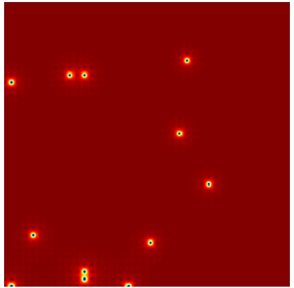
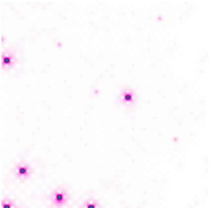
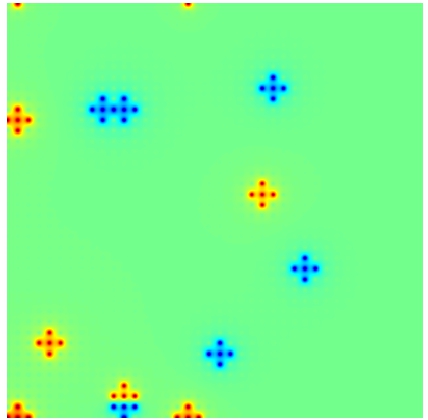
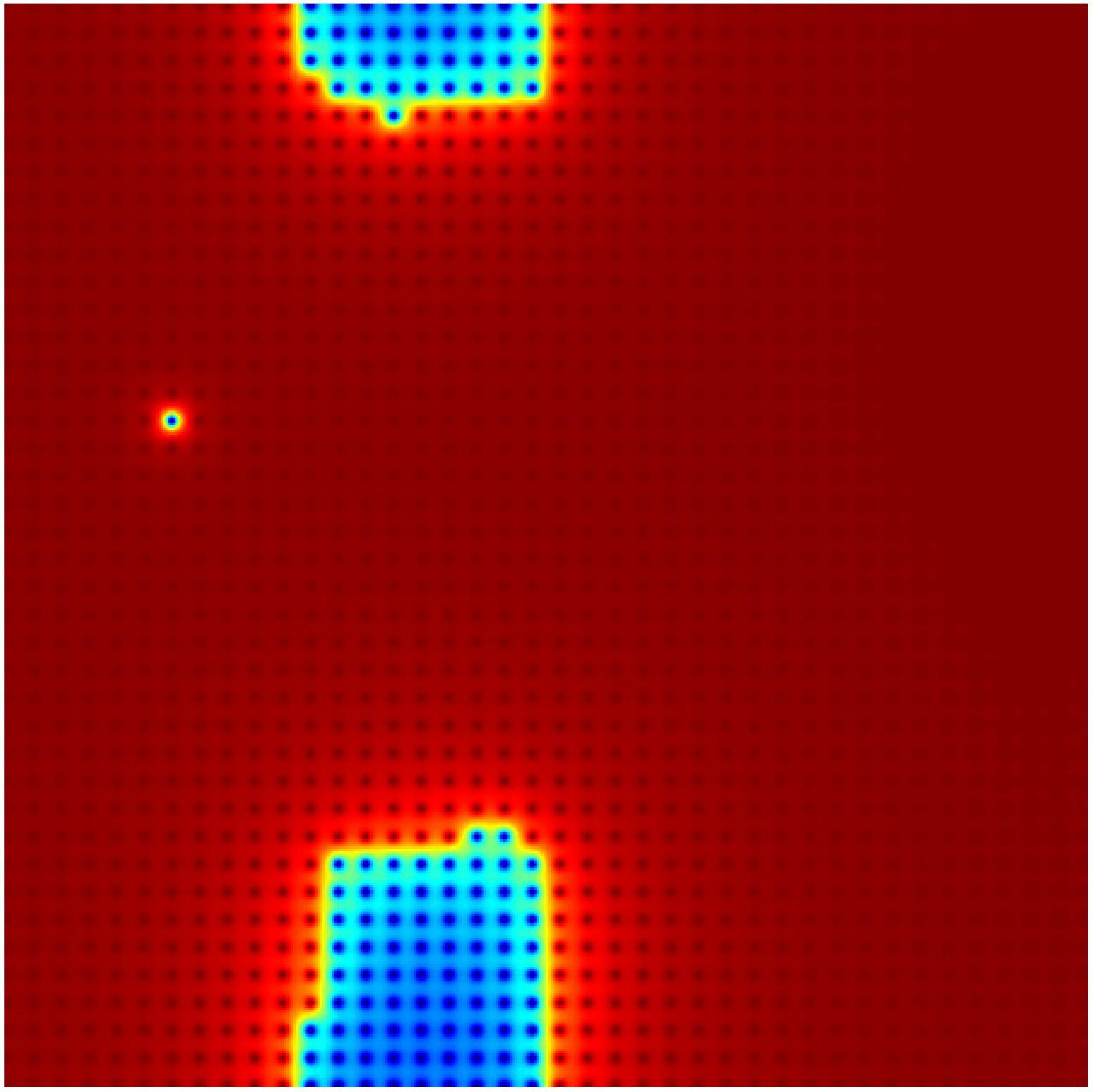
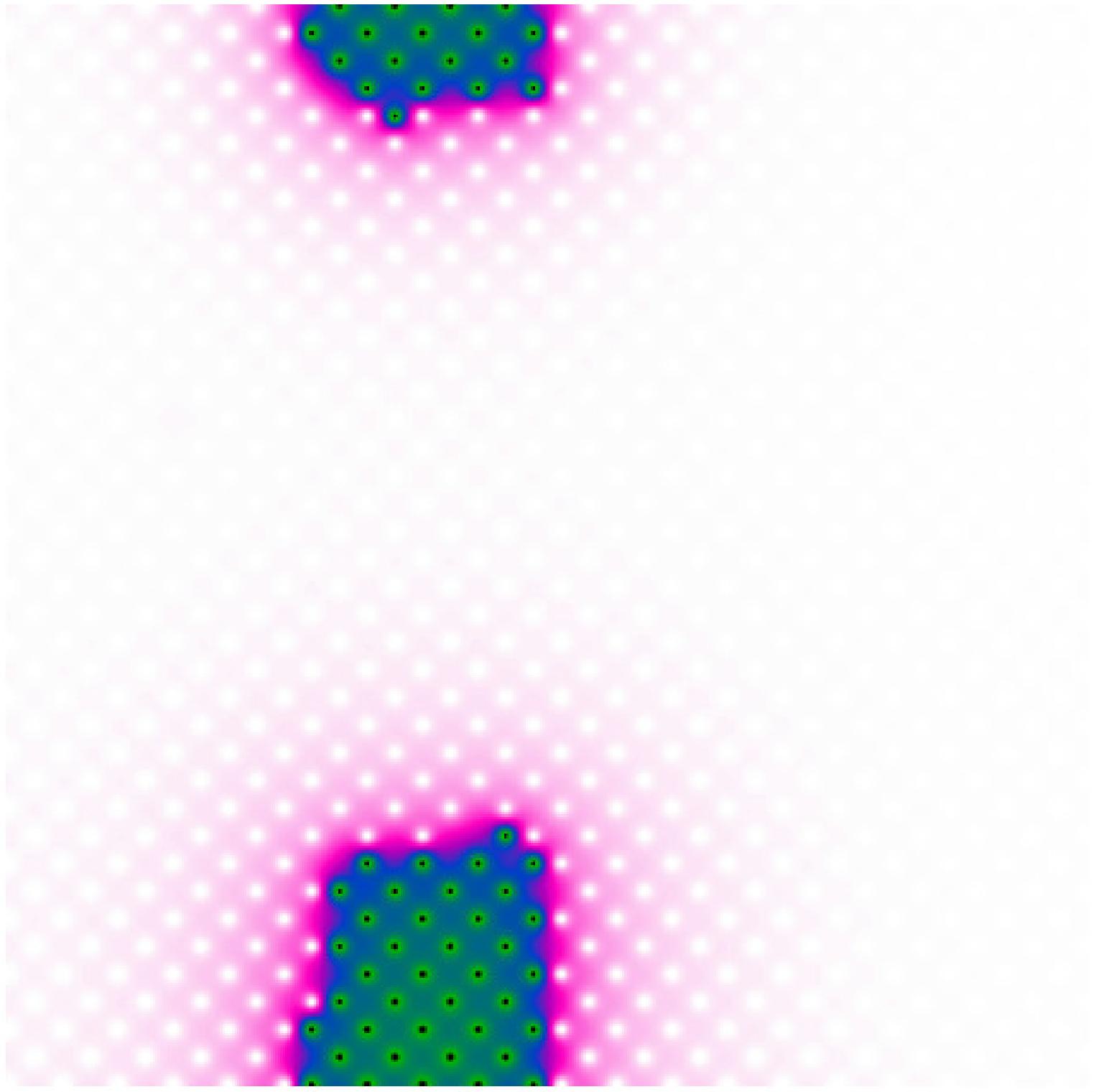
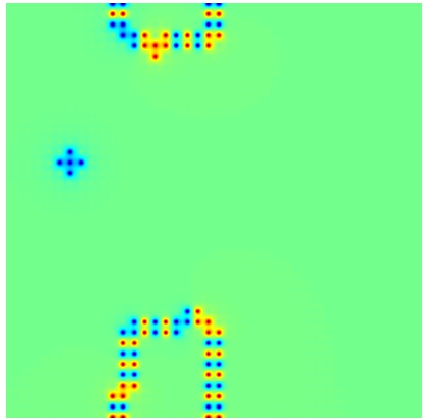
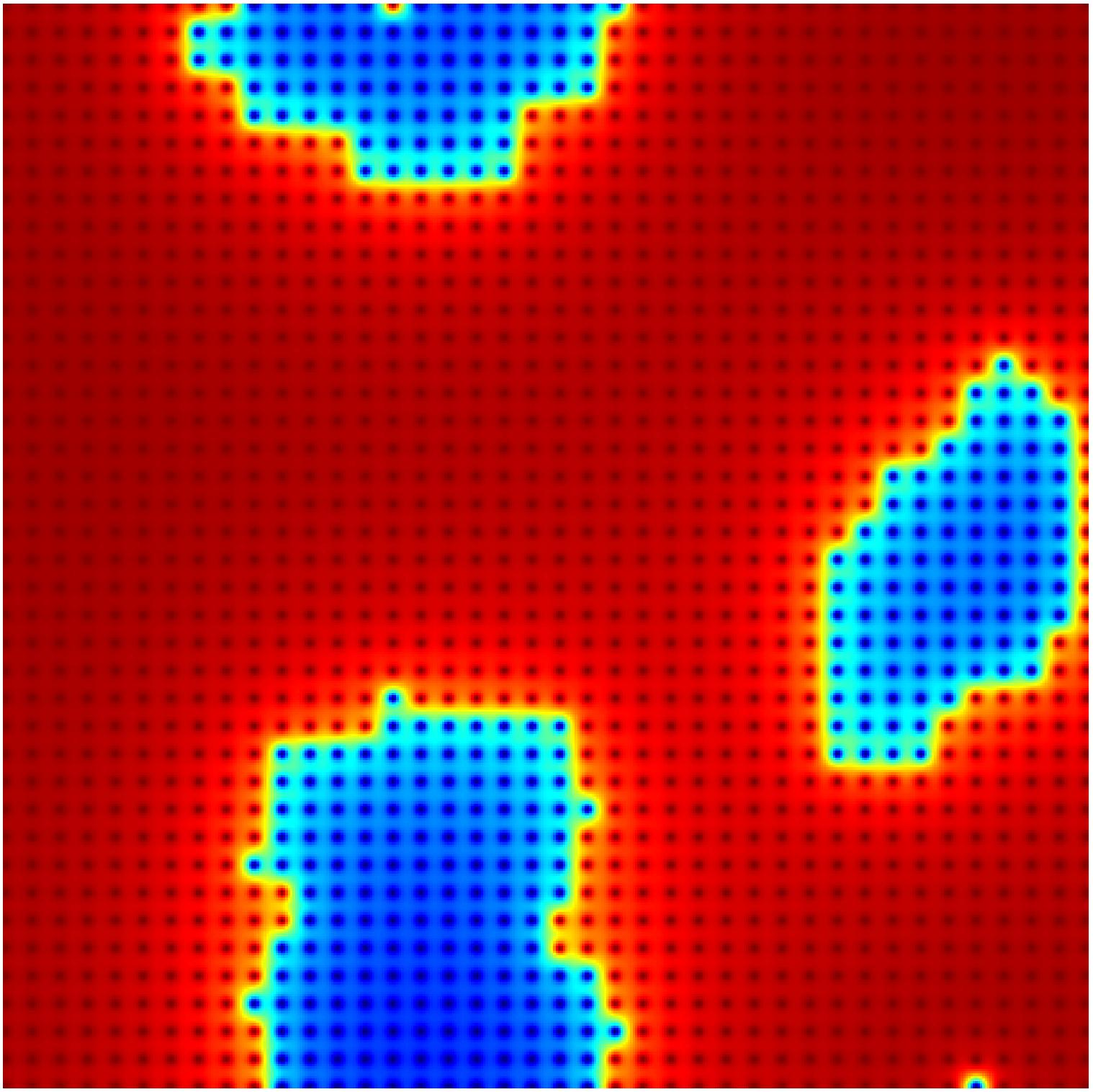
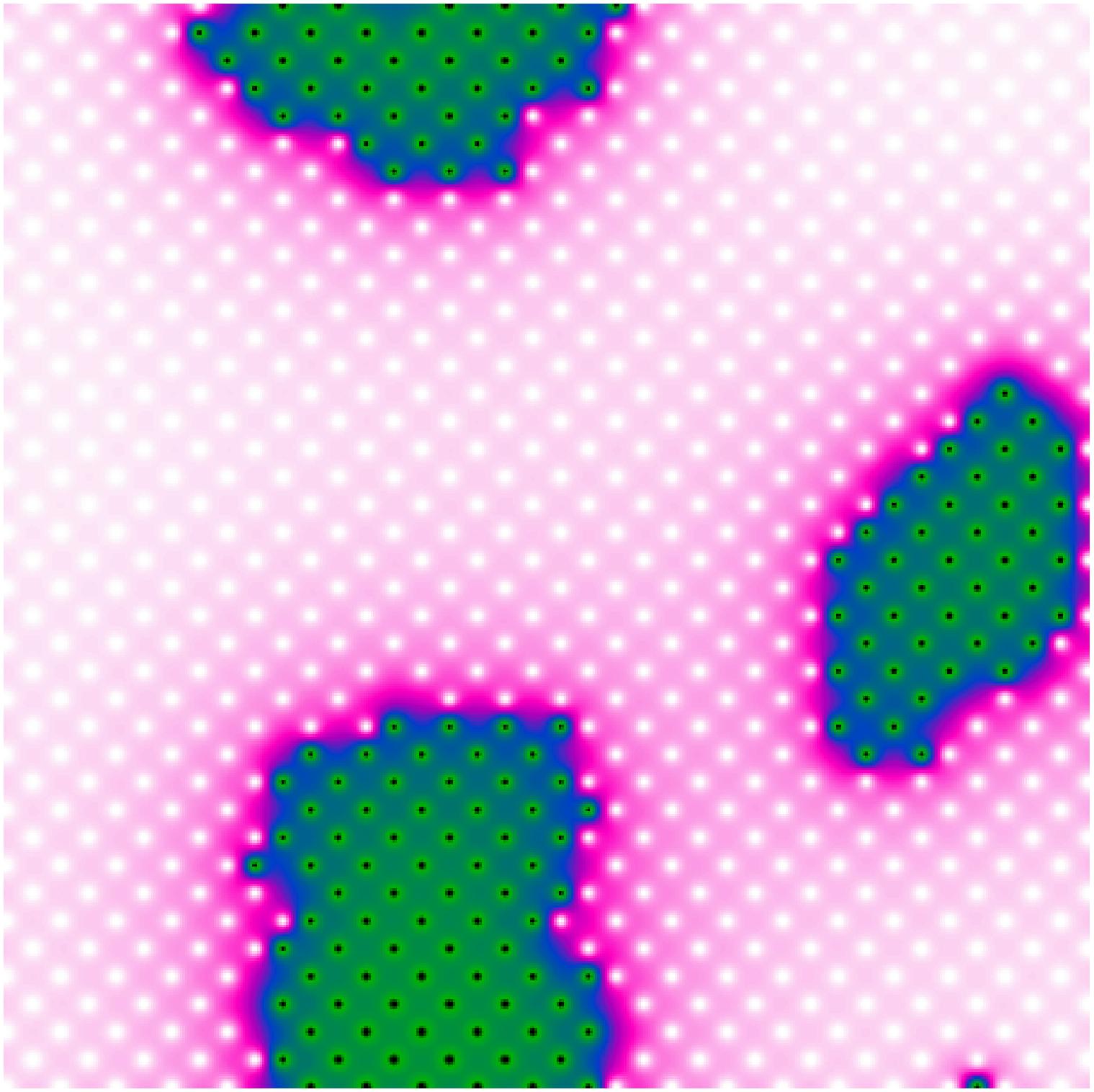
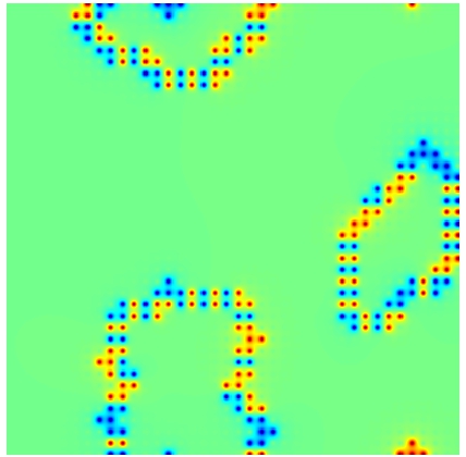
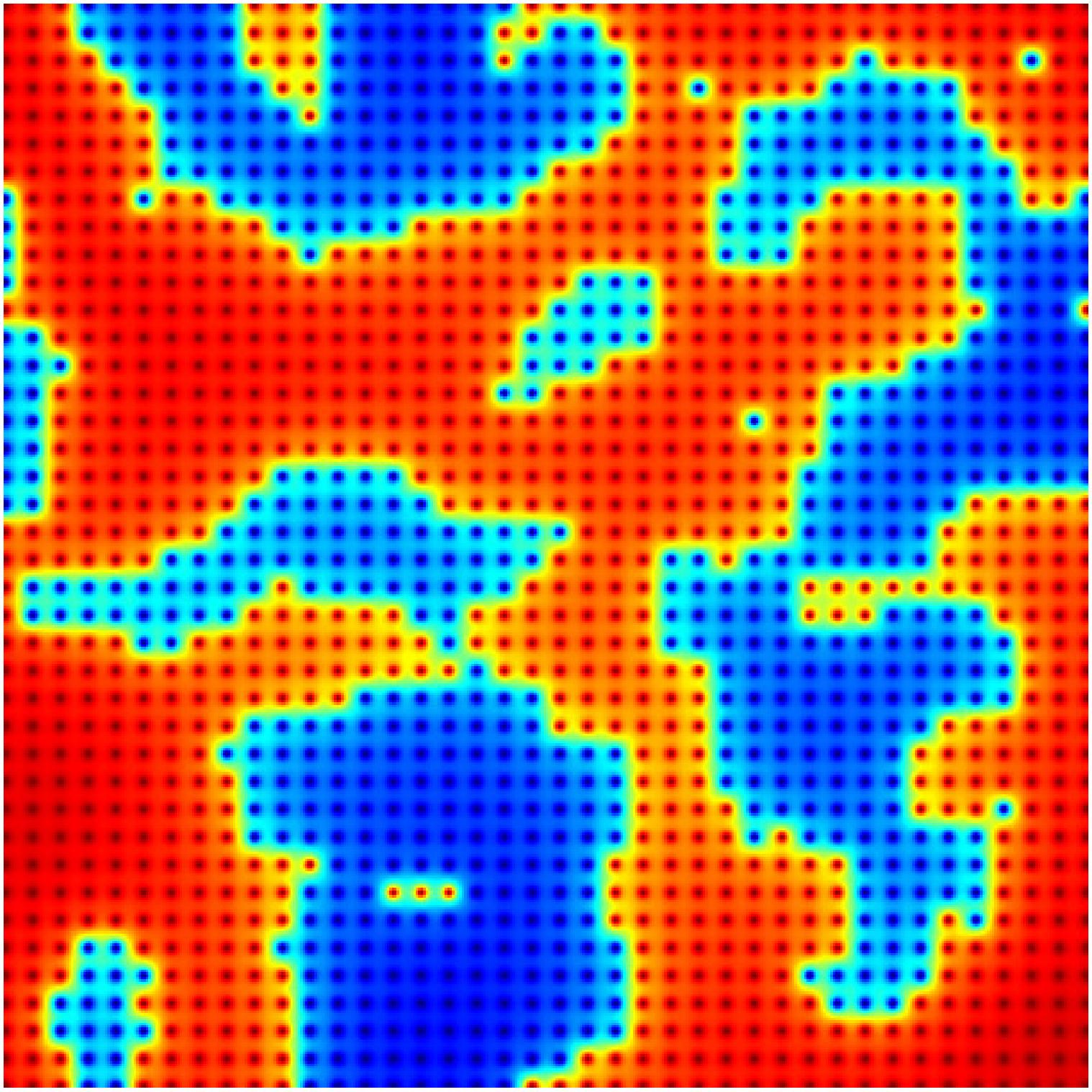
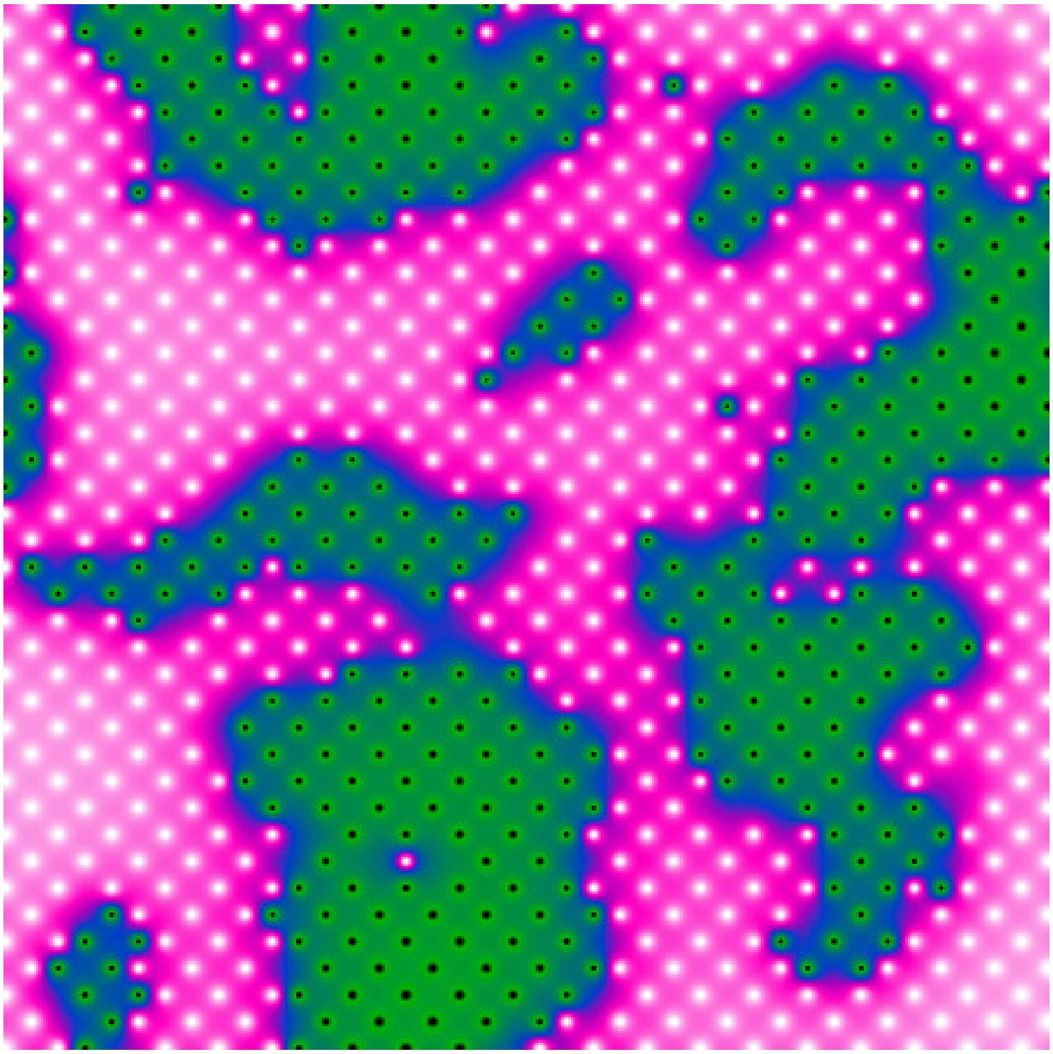
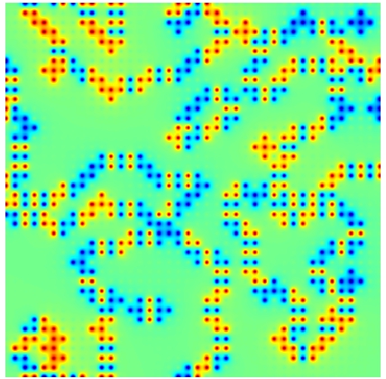
Figure 1: (Colour online) First column contains the structural motif for four disordered families with progressively increasing disorder (from top to bottom). We plot the $g(\bf{r_{i}})=(\eta_{i}-\frac{1}{2})e^{i\pi(x_{i}+y_{i})}$ . We denote the configurations as C1, C2, C3, C4 and the corresponding structural order parameter has values $S=0.98,~{}0.88,~{}0.59,~{}0.17$ from top to bottom. Second column shows the ground state spin overlap factor, $h_{i}=\bf{S_{0}}.\bf{S_{i}}$, where $\bf{S_{0}}$ is the left-lower-corner spin in the lattice. In the third column, we have shown the corresponding NN bond configurations. Here we have three different type of NN bonding present between B-B, B’-B’ and B-B’, represented by colours red, blue and green respectively in the plot. Lattice size is $40\times 40$.

Annealing the electron-spin system down to low temperature on a given structural motif leads to the magnetic ground states shown in the middle column of Fig.1. We plot the spin overlap factor, $h_{i}=\bf{S_{0}}.\bf{S_{i}}$, where $\bf{S_{0}}$ is the left-lower-corner spin in the lattice. The comparison of the first and second columns in Fig.1 indicate that the structural and magnetic domains coincide with each other. The third column of Fig.1 shows the NN structural partners. We have three possibilities: B-B, B’-B’ and B-B’, represented by colours red, blue and green respectively in the plot.

II.3 Effective Heisenberg Hamiltonian

Considering the difficulty in doing a spin-wave analysis on the full electronic-magnetic Hamiltonian (Eq. 1), we assume that the spin dynamics can be described by an $\it effective$ Heisenberg model

$$H_{eff}=\sum_{\{ij\}}J_{ij}\;{\bf S}_{i}.{\bf S}_{j}$$ (2)

where $\{\}$ represents the set of NN and next nearest neighbour (NNN) sites. $J_{ij}$ is the effective coupling (FM/AFM) between the local moments at ${\bf r}_{i}$ and ${\bf r}_{j}$ sites. In our two dimensional ASD configurations $J_{F}$ operates between two local moments when they are at the NNN position and $J_{AF}$ is active when the moments are at the NN position (a B-O-B arrangement). We have estimated the effective coupling $J_{F}$ and $J_{AF}$ as follows. For getting the FM coupling ($J_{F}$) we have considered the ordered double perovskite structure. We calculated the order parameter, i.e, the magnetic structure factor S($\bf{k}$) at ${\bf{k}}=(0,0)$, as a function of temperature for the full electronic Hamiltonian (Eq. 1) using Monte Carlo simulation. We then repeated the same procedure for the NNN FM Heisenberg Hamiltonian, defined on only the magnetic sites of the double perovskite. We found that for $J_{F}/t=-0.04$, two results matches very well.

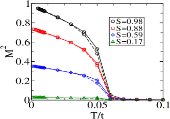
Figure 2: (Colour online) Comparison between the evolution of the spin structure factor S($\bf k$) at ${\bf k}=(0,0)$ with temperature for the spin configurations of various disorder families (from top to bottom) C1, C2, C3 and C4 obtained from the full electronic Hamiltonian with $J^{AF}S^{2}/t=0.08$ and the effective Heisenberg model with $J_{F}/t=-0.04$ and $J_{AF}/t=0.065$. Lattice size is $40\times 40$.

In order to get the AFM coupling we considered the ordered perovskite where both the B and B’ site carry a magnetic moment (mimicking SrFeO₃) and computed its AFM structure factor peak k=($\pi,\pi$). This model involves both electronic kinetic energy and Fe-Fe superexchange. We find that the result can be modelled via a Heisenberg model with $J_{AF}/t=0.065$.

Using the couplings inferred from these limiting cases, $J_{F}/t=-0.04$ and $J_{AF}/t=0.065$, we studied the bond disordered Heisenberg model for the antisite disordered DP magnet. We compared the FM structure factor peak S($\bf{k}$) at ${\bf k}$=(0,0) obtained from the disordered Heisenberg model with that from the full electronic Hamiltonian (Eq. 1). The Heisenberg result for the FM structure factor S(0,0) as a function of temperature matches very well, Fig.2, with the electronic Hamiltonian result for all ASD configurations. This gives us confidence in the usefulness of the Heisenberg model for spin dynamics.

III Spin dynamics

III.1 Spin-Wave Excitation

In this section we use the spin rotation technique fishmanJPCM21 to evaluate the spin-wave modes and dynamic structure factor at zero temperature. The effective Heisenberg model (Eq. 2) can be cast in a form useful for spin wave analysis by defining a local frame at each site so that the spins point along the $+z$ direction in the ground state. We can use ${\bar{\bf S}}_{i}=U_{i}{\bf S}_{i}$, where ${\bar{\bf S}}_{i}$ points along its local $z-$axis in the classical limit. The unitary rotation matrix $U_{i}$ for site ${\bf r}_{i}$ is given by

$$U_{i}=\left|\begin{array}[]{ccc}\cos(\theta_{i})\cos(\psi_{i})&\cos(\theta_{i})\sin(\psi_{i})&-\sin(\theta_{i})\\ -\sin(\psi_{i})&\cos(\psi_{i})&0\\ \sin(\theta_{i})\cos(\psi_{i})&\sin(\theta_{i})\sin(\psi_{i})&\cos(\theta_{i})\end{array}\right|,$$ (3)

where $\theta$ and $\psi$ are the Euler rotation angles. Now one can write the generalized Hamiltonian

$$H_{eff}=\sum_{\{ij\}}J_{ij}{\bar{\bf S}}_{i}.F_{ij}{\bar{\bf S}}_{j},$$ (4)

where $F_{ij}=U_{i}U_{j}$ is the overall rotation from one reference frame to another and its elements $F_{ij}^{\alpha\beta}$ can be obtained from Eq. (3).

Applying the approximate Holstein-Primakoff (HP) transformation in the large $S$ limit the spin operators in the local reference frame become: $\bar{S}_{i}^{+}=\sqrt{2S}\>b_{i}$, $\bar{S}_{i}^{-}=\sqrt{2S}\>b_{i}^{{\dagger}}$ and $\bar{S}_{i}^{z}=S-b_{i}^{{\dagger}}b_{i}$, where $b_{i}$ and $b_{i}^{{\dagger}}$ are the boson (magnon) annihilation and creation operators respectively. Only retaining the quadratic terms in $b$ and $b^{{\dagger}}$, which describe the dynamics of the non-interacting magnons and neglect magnon interaction terms of order $1/S$, the generalized Hamiltonian (Eq. 4) reduces to

$${\cal H}=\sum_{\{ij\}}[{\cal J}_{ij}(G_{ij}^{1}b_{i}^{{\dagger}}b_{j}+G_{ij}^{2}b_{i}b_{j}+h.c.)+f_{ij}(b_{i}^{{\dagger}}b_{i}+b_{j}^{{\dagger}}b_{j})],$$ (5)

where ${\cal J}_{ij}=SJ_{ij}/2$, $f_{ij}=-SJ_{ij}F_{ij}^{zz}$ and the rotation coefficients $G^{{}^{1}_{2}}=(F_{ij}^{xx}\pm F_{ij}^{yy})-i(F_{ij}^{xy}\mp F_{ij}^{yx})$. The Hamiltonian (5) is diagonalized by the transfermation

$$b_{i}=\sum_{n}(u_{n}^{i}c_{n}+v_{n}^{i^{*}}c_{n}^{{\dagger}}),$$ (6)

where $c^{{\dagger}}$ and $c$ are the quasiparticle operators. $u$ and $v$, which satisfy $\sum_{n}(u_{n}^{i}u_{n}^{j^{*}}-v_{n}^{i^{*}}v_{n}^{j})=\delta_{ij}$ ensuring the bosonic character of the quasiparticles are obtained from

$$\left(\begin{array}[]{cc}A_{ij}&B_{ij}^{*}\\ B_{ij}&A_{ij}^{*}\end{array}\right)\left(\begin{array}[]{c}u_{n}^{j}\\ v_{n}^{j}\end{array}\right)=\omega_{n}\left(\begin{array}[]{cc}\delta_{ij}&0\\ 0&-\delta_{ij}\end{array}\right)\left(\begin{array}[]{c}u_{n}^{j}\\ v_{n}^{j}\end{array}\right),$$ (7)

where $A_{ij}={\cal J}_{ij}(G_{ij}^{1}+G_{ji}^{1^{*}})+\epsilon_{i}\delta_{ij}$, $B_{ij}={\cal J}_{ij}(G_{ij}^{2}+G_{ji}^{2})$ and $\epsilon_{i}=\sum_{j}(f_{ij}+f_{ji})$. Now the spin-spin correlation function can be evaluated using the magnon energies and wavefunctions obtained from Eq. (7), where the excitation eigenvalues $\omega_{n}\geq 0$.

III.2 Dynamical Structure Factor

A neutron scattering experiment measures the spin-spin correlation function in Fourier and frequency space $S({\bf k},\omega)$ to describe the spin dynamics of the magnetic systems on an atomic scale. From ${\bf S}_{i}=U_{i}^{-1}{\bar{\bf S}}_{i}$ one can express $S_{i}^{\alpha}=\sum_{\mu}U_{i}^{{\mu\alpha}^{*}}{\bar{S}_{i}^{\mu}},$ where $\alpha$ and $\mu$ represents the $x$, $y$, and $z$ components. Now applying the approximate HP transformation to the rotated spins one can write

$$S_{i}^{\beta}=p_{i}^{\beta}b_{i}+q_{i}^{\beta}b_{i}^{{\dagger}}+r_{i}^{\beta}(S-b_{i}^{{\dagger}}b_{i}),$$ (8)

where $\beta=+$, $-$ and $z$, and $p,q$ and $r$ are the rotation coefficients (given in the Appendix).

Putting Eq. (6) in (8) the space time spin-spin correlation function can be written as

$$S_{i}^{\alpha}(t)S_{j}^{\beta}(0)=\sum_{mn}[A_{{}^{mn}_{ij}}^{\alpha\beta}c_{m}^{{\dagger}}(t)c_{n}(0)+B_{{}^{mn}_{ij}}^{\alpha\beta}c_{m}(t)c_{n}^{{\dagger}}(0)],$$ (9)

where the coefficients A and B are expressed in the Appendix. In Fourier and frequency space

$$S^{\alpha,\beta}({\bf k},\omega)=\frac{1}{N}\int dte^{-i\omega t}\sum_{ij}e^{i{\bf k}.({\bf r}_{i}-{\bf r}_{j})}\langle S_{i}^{\alpha}(t)S_{j}^{\beta}(0)\rangle.$$ (10)

and the total spin-spin correlation function

$$S({\bf k},\omega) = \frac{1}{2}[S^{+,-}({\bf k},\omega)+S^{-,+}({\bf k},\omega)]+S^{z,z}({\bf k},\omega)$$

$$= \sum_{l}W_{\bf k}^{l}\delta(\omega-\omega_{l}),$$

where the coefficient of the delta function

$$W_{\bf k}^{l}=\frac{1}{N}\sum_{ij}{\cal B}_{ij}^{l}e^{i{\bf k}.({\bf r}_{i}-{\bf r}_{j})}$$ (11)

is the SW weight with ${\cal B}_{ij}^{l}=\frac{1}{2}(B_{{}^{ll}_{ij}}^{+-}+B_{{}^{ll}_{ij}}^{-+})+B_{{}^{ll}_{ij}}^{zz}$. $W_{\bf k}^{l}$ is observed as the intensity of magnon spectrum in the neutron scattering experiment.

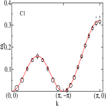
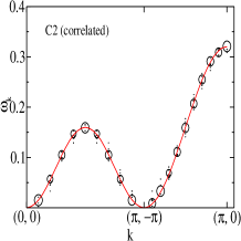
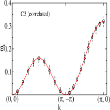
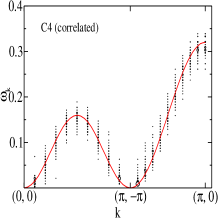
Figure 3: (Colour online) Spin-wave spectrum along main symmetry directions of the Brillouin zone for spin configurations C1, C2, C3 and C4 ($x$ = 0.01, 0.11, 0.21 and 0.41 respectively). shown in Fig.1 With increasing ASD from C1 to C4 the spectrum becomes broader for a fixed value of momentum ${\bf k}$. Here $J_{F}=-0.04$, $J_{AF}=0.065$, and lattice size is $40\times 40$.

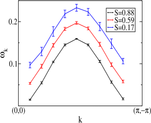
Figure 4: (Colour online) Mean spin wave energy ${\bar{\omega}}_{\bf k}$ (dots) and spin-wave width $\Delta\omega_{\bf k}$ (bars), defined in the text, for the correlated antisite configurations C2-C4. The curves are vertically shifted for clarity.

IV Results and Discussion

We start by presenting the results for magnons in the configurations C1-C4 shown in Fig.1 and then move to an analysis of the linewidth, the estimation of domain size, and the contrast with uncorrelated disorder.

IV.1 Results for AF coupled domains

Fig.3 shows the magnon spectra of C1-C4 with obtained from the Heisenberg model with the FM and AFM couplings discussed earlier. In a model with only FM couplings, i.e., no disorder, we would have obtained only the red curve, $\omega^{0}_{\bf k}$, for propagating magnons. The striking feature in all these panels is how closely the mean energy of the magnons follow $\omega^{0}_{\bf k}$ despite the large degree of mislocation in C2 and C3 and maximal disorder ($x\sim 0.5$) in C4 (refer to the spatial plots in Fig.1). The broadening, although noticeable in C4, does not obscure the basic dispersion.

Fig.4 quantifies the mean energy and broadening by computing:

$${\bar{\omega}}_{\bf k}=\int~{}S({\bf k},\omega)\omega d\omega$$

$$[{\Delta\omega_{\bf k}}]^{2}=[\int~{}S({\bf k},\omega)\omega^{2}d\omega]-{\bar{\omega}}^{2}_{\bf k}$$

We have shown these two quantities for the C2-C4 structures in Fig.1. The ${\bar{\omega}}_{\bf k}$ have been vertically shifted for clarity and the ${\Delta\omega_{\bf k}}$ are superposed as ‘error bars’ on these. It is clear that even in the most disordered sample (C4), where the mislocation $x\sim 0.4$, the broadening is only a small fraction of the magnon energy. This will be an indicator when we discuss spin waves in an uncorrelated disorder background.

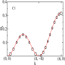
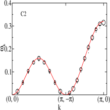
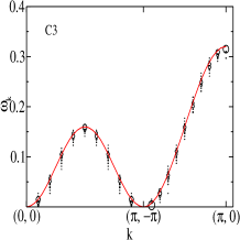
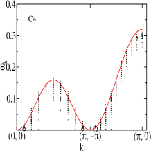
Figure 5: (Colour online) Spin-wave spectra along main symmetry directions of the Brillouin zone for spin configurations C1, C2, C3 and C4 shown in Fig.1 ($x$ = 0.01, 0.11, 0.21 and 0.41 respectively). Increasing fractional weakly coupled domain boundary spins from C1 to C4 enhances the SW softening near the ZB along $[\pi,0]$ and the spectrum also becomes broader for a given ${\bf k}$. Here $J_{F}=-0.04$, $J_{AF}=0$, and lattice size is $40\times 40$.

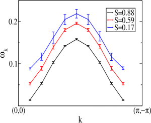
Figure 6: (Colour online) Mean spin wave energy ${\bar{\omega}}_{\bf k}$ (dots) and spin-wave width $\Delta\omega_{\bf k}$ (bars) for C2-C4 now with $J_{AF}=0$, i.e, decoupled domains. The curves are vertically shifted for clarity.

IV.2 Broadening: impact of domain size

There are two ingredients responsible for the spectrum that one observes in Fig.3, (i) the domain structure, and (ii) the AF coupling across the domains. To deconvolve these effects and have a strategy for inferring domain size from neutron data, we studied a situation where we set $J_{AF}=0$ in the Heisenberg model defined on the structures C1-C4. In that case we will have decoupled FM domains without any antiparallel spin orientation between them. We think this is a interesting scheme to explore since the AF bonds are limited to the domain boundaries and is not equal to the number of mislocated sites.

Fig.5 shows the overall magnon spectrum for this case, using the same convention as in Fig.3, while Fig.6 quantifies the mean energy and broadening in this ‘decoupled domain’ case. The absence of $J_{AF}$ does not seem to make a significant difference to the spectrum as a comparison of Fig.4 and Fig.6 reveal.

     

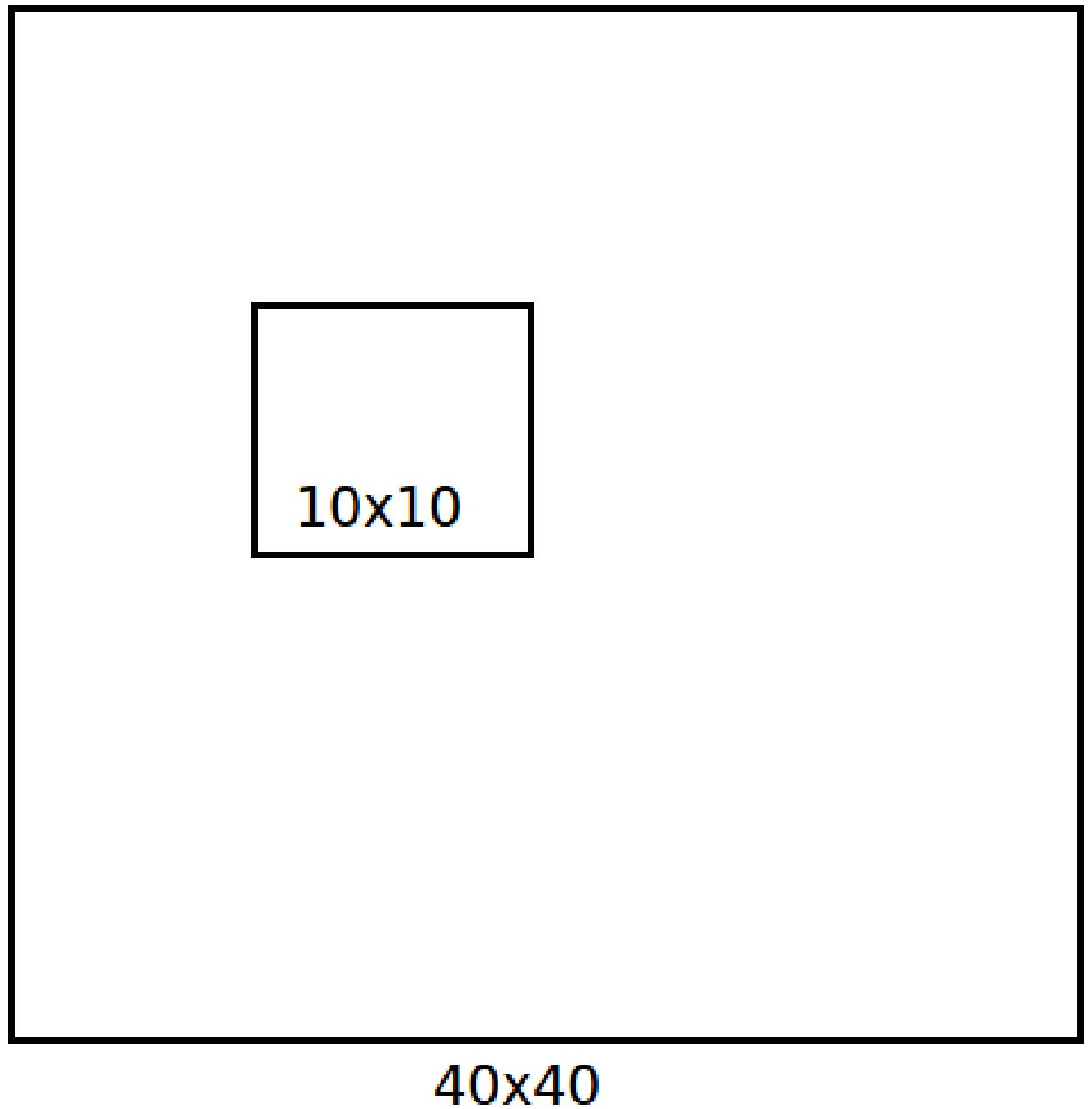
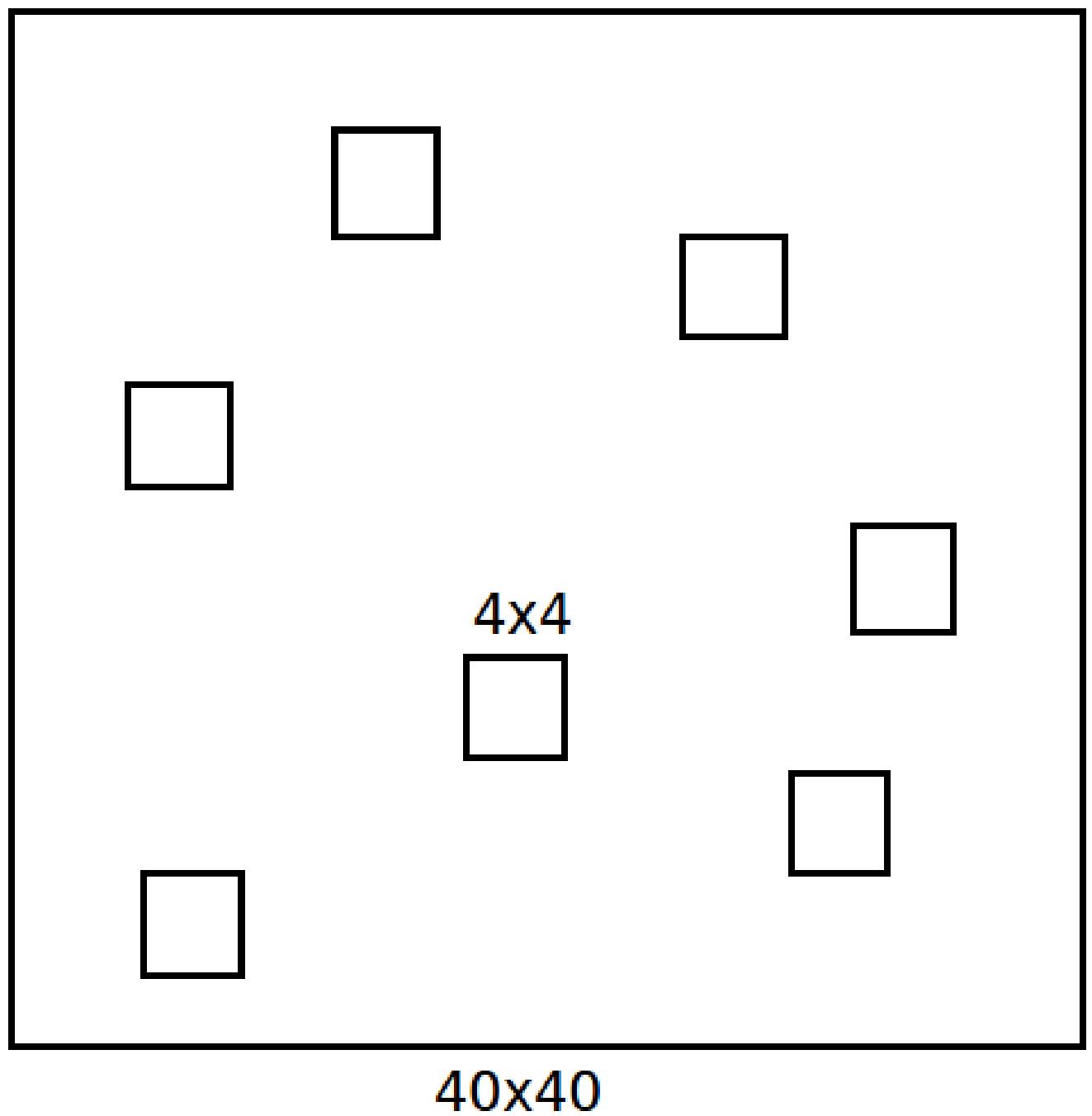
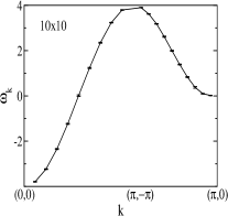
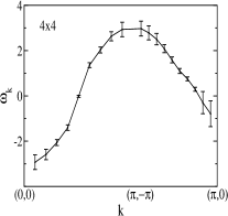
Figure 7: (Colour online) Modelling C2 in terms of a domain of size $10\times 10$ (left) and of seven domains of size $4\times 4$ (right). The corresponding mean energy and broadening are shown below.

This correspondence, valid even in C4, suggests the following: (i) most of the spectral features arise from the domain structure, and the associated confinement of spin waves, rather than the AF coupling, and (ii) we can proceed with a much simpler modelling of the spectrum and estimation of domain size without invoking the complicated BdG formulation that AFM coupling requires.

Essentially, much can be learnt from ‘tight binding’ models defined on appropriate stuctures, as happens for FM states, without having to invoke the ‘pairing’ terms that arise for AF coupling. A modelling of the full dispersion will require the AF terms as well, but the inference about presence of domains, and an estimate of their size, need not. We proceed with this next.

To make some progress in estimating the typical domain size we need a few assumptions; (i) the total degree of mislocation, $x$, should be known, based on the bulk magnetisation measurement. (ii) If the overall system size in $L\times L$ (or equivalent in a 3D model), the number of mislocated sites would be $xL^{2}$. (iii) If the domain size is $L_{d}$ then the number of domains within the $L\times L$ area is $N_{d}\sim xL^{2}/L_{d}^{2}$. In reality domains need not have one single size, as C2-C4 indicate, but we need the assumption to make some headway. (iv) We need to locate these $N_{d}$ domains randomly, in a non overlapping manner, within the $L\times L$ system, and average the spectrum obtained over different realisations of domain location.

This scheme, carried out for various $L_{d}$, can be compared to the full $S({\bf k},\omega)$ data to get a feel for the appropriate $L_{d}$. We show the result below for such a tight binding exploration for the C2 configuration, modelled in terms of different domain distributions that respect the same overall mislocation.

When we compare the ratio of mean broadening to bandwidth obtained at different values of $L_{d}$ (and so $N_{d}$) with that for the real data, Fig.4, it turns out that $L_{d}=10$ provides a best estimate. It also reasonably describes the broadening at stronger disorder, C3 and C4, where of course $N_{d}$ is larger. An analytic feel for these results can be obtained by considering the modes of a square size $L_{d}\times L_{d}$ under open boundary conditions.

IV.3 Contrast with uncorrelated antisites

In modelling the antisite disorder much of the earlier work in the field assume the defect locations to be random. We have followed the experimentally motivated path which suggests that the mislocated sites themselves form an ordered structure separated from the parent (or majority) by an antiphase boundary. The sources of scattering are the boundary between these domains rather than random point defects. Since much of double perovskite modelling has assumed the random antisite situation it is worth exploring the differences in the magnon spectrum between correlated and uncorrelated antisites.

We have already seen the results for correlated disorder for different degrees of mislocation, $x$. We generated uncorrelated antisite configurations with the same $x$ by starting with ordered configurations and randomly exchanging B and B’ till the desired degree of disorder is reached. These configurations naturally do not have any structural domains. Annealing the full electronic Hamiltonian on these configurations, call them $C^{\prime}_{1},~{}C^{\prime}_{2},..$, etc, down to low $T$, leads to the magnetic ground states. The ground states are disordered ferromagnets but without any domain pattern. We computed the magnon lineshape in these configurations, and, for illustration, show the results for $C^{\prime}_{2}$ and $C^{\prime}_{3}$ side by side with their correlated counterparts $C_{2}$ and $C_{3}$.

There is a striking increase in the magnon line width (or $\Delta{\omega}_{\bf k}$) in the uncorrelated case. There is almost nine fold increase in the magnon line width in $C_{2}$ and six fold in $C_{3}$ of the uncorrelated disorder with respect to the correlated disorder case.

      

      

  

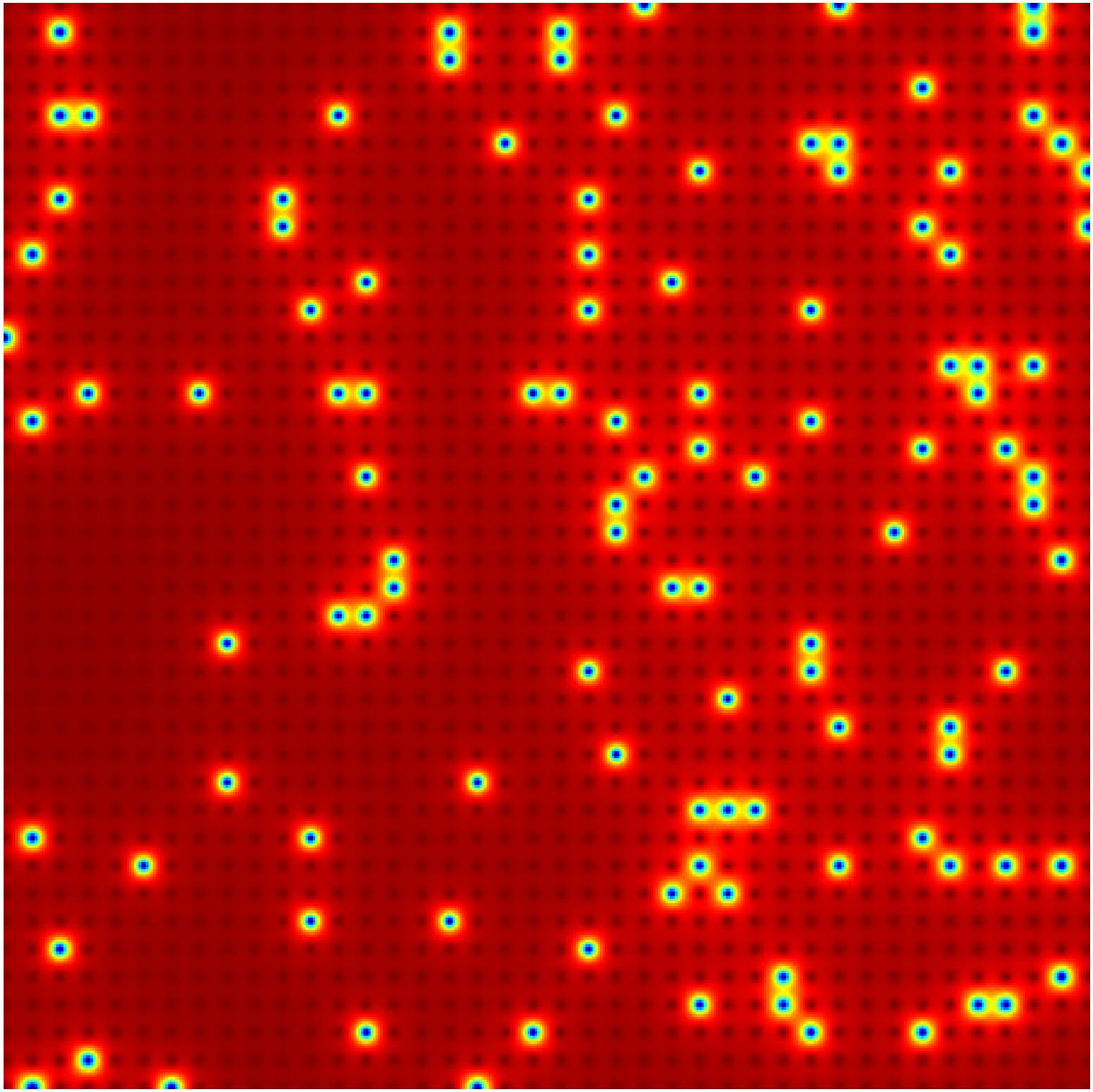
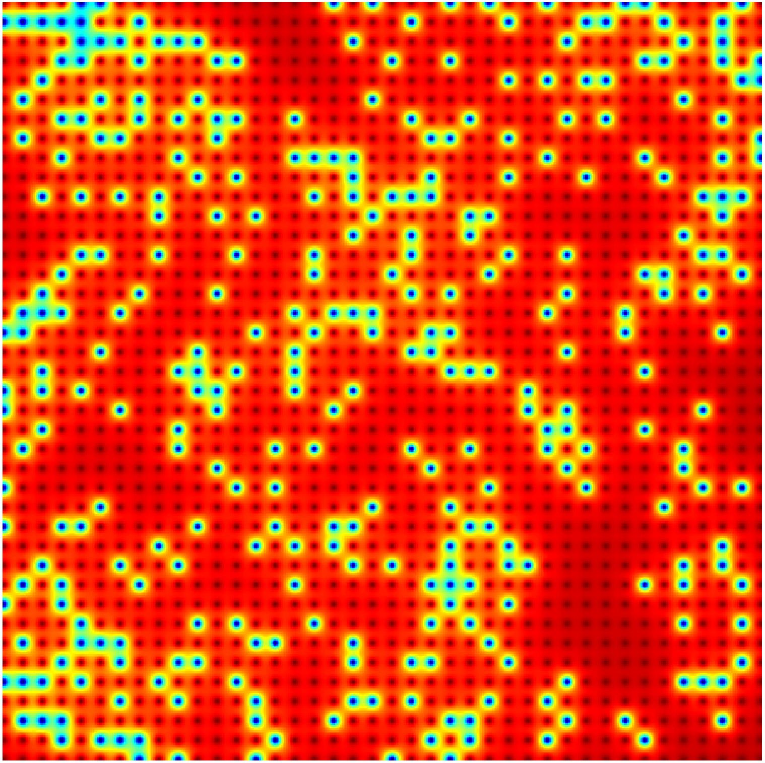
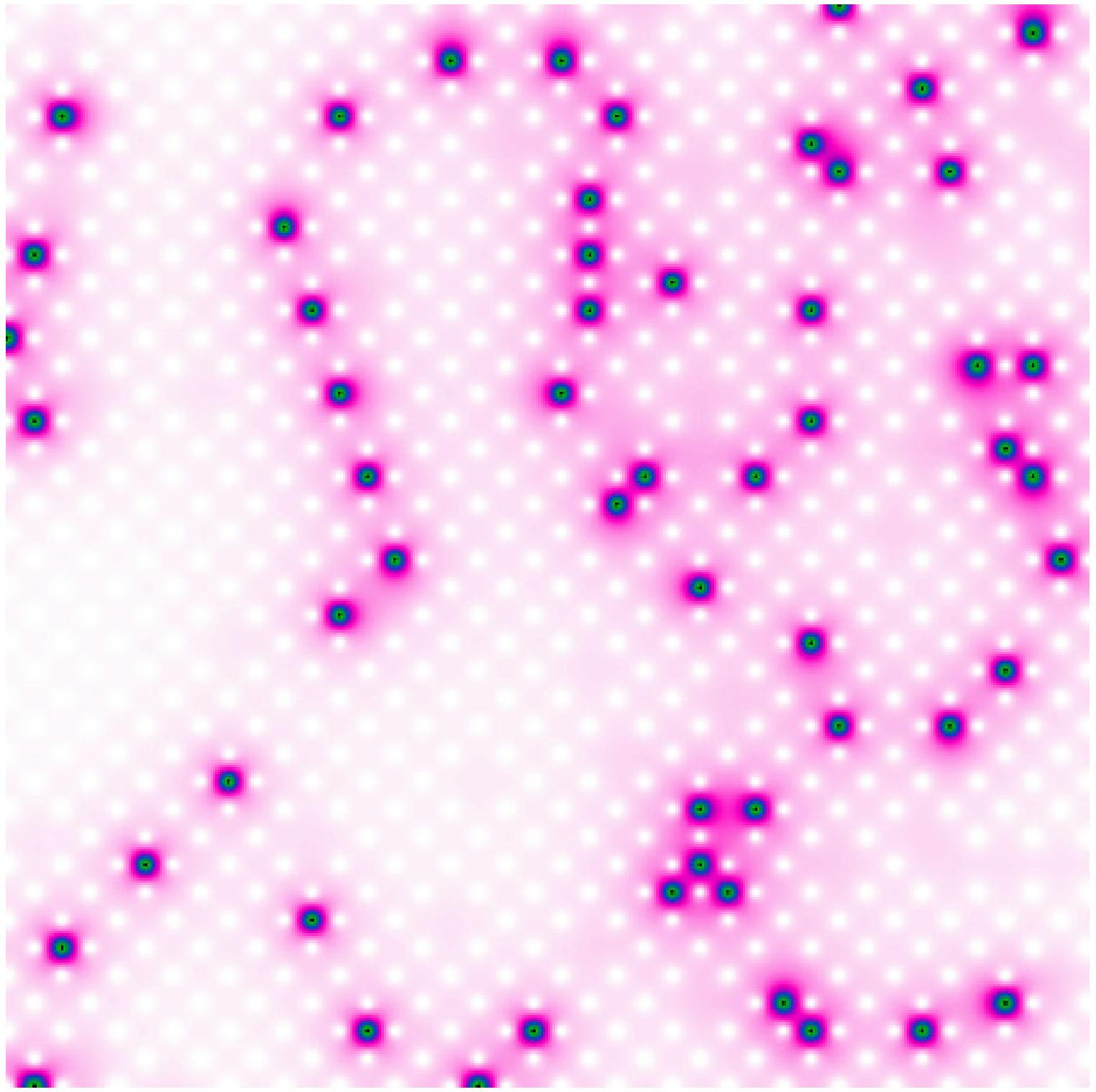
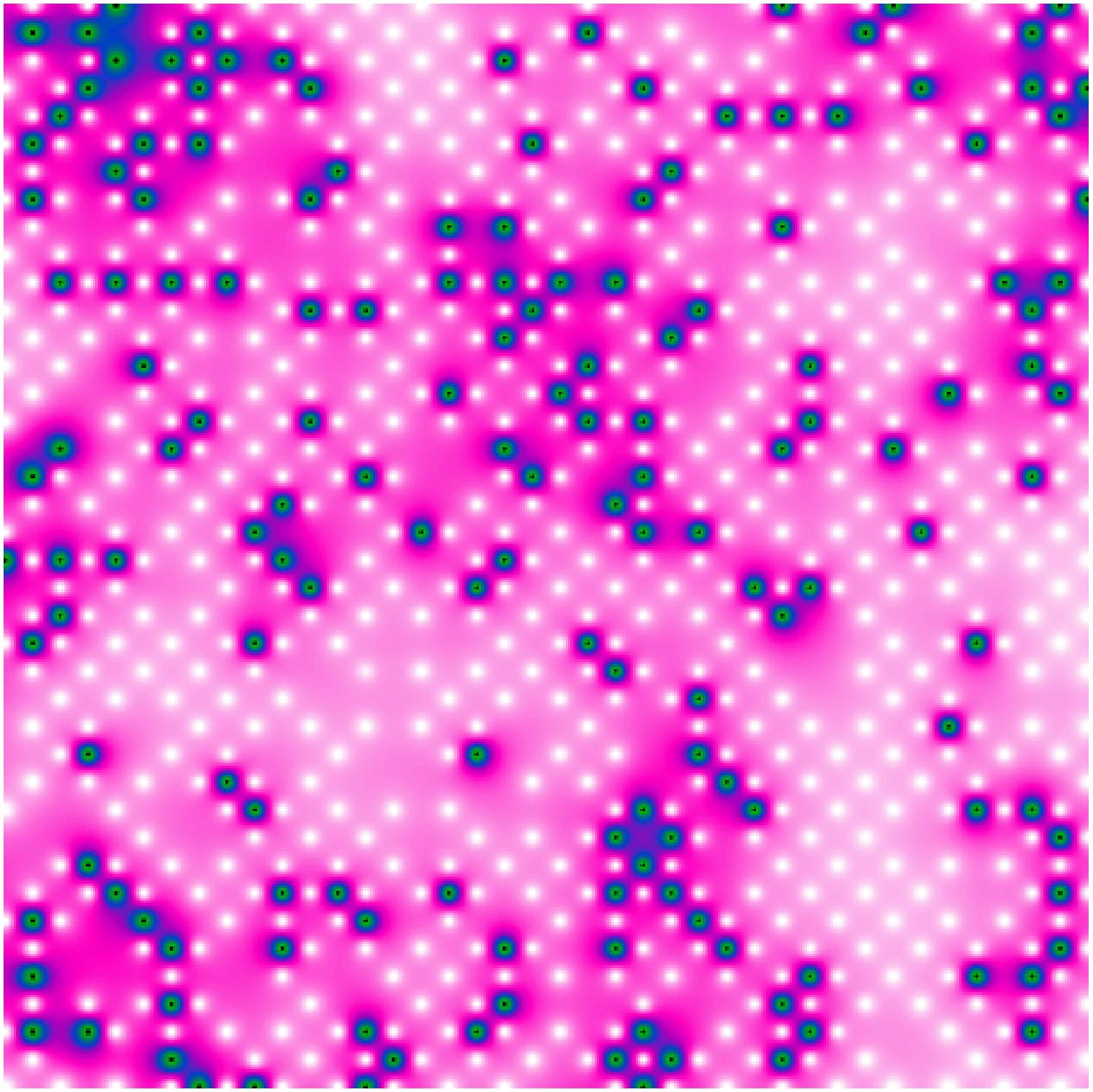
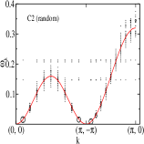
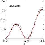
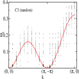
Figure 8: The left set of panels correspond to mislocation $x=0.11$ where we compare the magnon spectrum for uncorrelated disorder (left) with correlated disorder (C2) right. the top panels refer to the structural pattern, the middle to the magnetic ground state, and the bottom to the magnon response. The right set of panels refer to $x=0.21$, and the same indicators as for the left panels. Notice the remarkably broader lineshape for the uncorrelated disorder case where it is difficult to make much of a correspondence with the clean dispersion.

V Conclusion

We have studied the dynamical magnetic structure factor of a double perovskite system taking into account the basic ferromagnetic ordering tendency and the defect induced local antiferromagnetic correlations. We used structural motifs that correspond to correlated disorder, obtained from an annealing process. The results on magnon energy and broadening reveal that even at very large disorder, the existence of domain like structure ensures that the response has a strong similarity to the clean case. We tried out a scheme for inferring the domain size from the spin wave damping, so that experimenters can make an estimate of domains without having spatial data, and find it to be reasonably successful. We also highlight how the common assumption about random antisites, that is widely used in modelling these materials, would lead to a gross overestimate of magnon damping. In summary, dynamical neutron scattering can be a direct probe of the unusual ferromagnetic state in these materials and confirm the presence of correlated antisites.

VI Acknowledgement

We acknowledge use of the High Performance Computing facility at HRI. PM thanks the DAE-SRC Outstanding Research Investigator grant, and the DST India (Athena) for support.

VII appendix

The rotation coefficients are

$$\begin{array}[]{c}p_{i}^{\pm}=\sqrt{\frac{S}{2}}{(U_{i}^{xx}\pm U_{i}^{yy})-i(U_{i}^{yx}\mp U_{i}^{xy})}\\ q_{i}^{\pm}=\sqrt{\frac{S}{2}}{(U_{i}^{xx}\mp U_{i}^{yy})+i(U_{i}^{yx}\pm U_{i}^{xy})}\\ r_{i}^{\pm}=U_{i}^{zx}\pm iU_{i}^{zy}\\ p_{i}^{z}=U_{i}^{xz}-iU_{i}^{yz}\\ q_{i}^{z}=U_{i}^{xz}+iU_{i}^{yz}\\ r_{i}^{z}=U_{i}^{zz}.\end{array}$$ (12)

And the structure factor coefficients are

$$\begin{array}[]{c}A_{{}^{mn}_{ij}}^{\alpha\beta}=q_{i}^{\alpha}p_{j}^{\beta}u_{i}^{m^{*}}u_{j}^{n}+p_{i}^{\alpha}q_{j}^{\beta}v_{i}^{m^{*}}v_{j}^{n}+p_{i}^{\alpha}p_{j}^{\beta}v_{i}^{m^{*}}u_{j}^{n}\\ +q_{i}^{\alpha}q_{j}^{\beta}u_{i}^{m^{*}}v_{j}^{n}-S\times r_{i}^{\alpha}r_{j}^{\beta}(u_{i}^{m^{*}}u_{i}^{n}+u_{j}^{m^{*}}u_{j}^{n})\\ B_{{}^{mn}_{ij}}^{\alpha\beta}=q_{i}^{\alpha}p_{j}^{\beta}v_{i}^{m}v_{j}^{n^{*}}+p_{i}^{\alpha}q_{j}^{\beta}u_{i}^{m}u_{j}^{n^{*}}+p_{i}^{\alpha}p_{j}^{\beta}u_{i}^{m}v_{j}^{n^{*}}\\ +q_{i}^{\alpha}q_{j}^{\beta}v_{i}^{m}u_{j}^{n^{*}}-S\times r_{i}^{\alpha}r_{j}^{\beta}(v_{i}^{m}v_{i}^{n^{*}}+v_{j}^{m}v_{j}^{n^{*}}).\end{array}$$ (13)

References

- (1) For reviews, see D. D. Sarma, Current Op. Solid St. Mat. Sci.,5, 261 (2001), D. Serrate, J. M. de Teresa and M. R. Ibarra, J. Phys. Cond. Matt. 19, 023201 (2007).
- (2) K.-I. Kobayashi, T. Kimura, H. Sawada, K. Terakura and Y. Tokura, Nature 395, 677 (1998).
- (3) Y. Tomioka, T. Okuda, Y. Okimoto, R. Kumai, K.-I. Kobayashi, and Y. Tokura, Phys. Rev. B 61, 422 (2000).
- (4) T. Asaka, X. Z. Yu, Y. Tomioka, Y. Kaneko, T. Nagai, K. Kimoto, K. Ishizuka, Y. Tokura, and Y. Matsui, Phys Rev B 75, 184440 (2007).
- (5) C. Meneghini, Sugata Ray, F. Liscio, F. Bardelli, S. Mobilio, and D. D. Sarma, Phys. Rev. Lett. 103, 046403 (2009).
- (6) M. Hennion, et al, Phys. Rev. Lett. 94, 057006 (2005).
- (7) S. Petit, et al, Phys. Rev. Lett. 102, 207201 (2009).
- (8) V. N. Singh and P. Majumdar, Europhys. Lett. 94, 47004 (2011).
- (9) P. Sanyal, S. Tarat, and P. Majumdar, Eur. Phys. J. B 65, 39 (2008).
- (10) S. Kumar and P.Majumdar, Eur. Phys. J. B 50, 571-579 (2006).
- (11) R. S. Fishman, J. Phys. Cond. Mat. 21, 216001 (2009).
- (12) P. V. Hendriksen, S. Linderoth, and P.-A. Lindgård, J. Phys. Cond. Mat. 5, 5675 (1993), Phys. Rev. B 48, 7259 (1993).