Decoherence in two-dimensional quantum walks using four- and two-state particles

Abstract

We study the decoherence effects originating from state flipping and depolarization for two-dimensional discrete-time quantum walks using four-state and two-state particles. By quantifying the quantum correlations between the particle and position degree of freedom and between the two spatial ($x-y$) degrees of freedom using measurement induced disturbance (MID), we show that the two schemes using a two-state particle are more robust against decoherence than the Grover walk, which uses a four-state particle. We also show that the symmetries which hold for two-state quantum walks breakdown for the Grover walk, adding to the various other advantages of using two-state particles over four-state particles.

I Introduction

Quantum walks are a close quantum analog of classical random walks, in which the evolution of a particle is given by a series of superpositions in position space Ria58 ; Fey86 ; Par88 ; LP88 ; ADZ93 . Recently they have emerged as an efficient tool to carry out quantum algorithms Kem03 ; Amb03 and have been suggested as an explanation for wavelike energy transfer within photosynthetic systems ECR07 ; MRL08 . They have applications in the coherent control of atoms and Bose-Einstein condensates in optical lattices CL08 ; Cha11a , the creation of topological phases KRB10 , and the generation of entanglement GC10 . Quantum walks therefore have the potential to serve as a framework to simulate, control and understand the dynamics of a variety of physical and biological systems. Experimental implementations of quantum walks in last few years have included NMR DLX03 ; RLB05 ; LZZ10 , cold ions SMS09 ; ZKG10 , photons PLP08 ; PLM10 ; SCP10 ; BFL10 ; SCP11 ; SSV12 , and ultracold atoms KFC09 , which has drawn further interest of the wider scientific community to their study.

The two most commonly studied forms of quantum walks are the continuous-time FG98 and the discrete-time evolutions ADZ93 ; DM96 ; ABN01 ; NV01 ; Kon02 ; BCG04 ; CSL08 . In this work we will focus on the discrete-time quantum walk and just call it quantum walk for simplicity. If we consider a one-dimensional (1D) example of a two-state particle initially in the state

$$|\Psi_{\rm in}\rangle=\left(\cos(\delta/2)|0\rangle+e^{i\eta}\sin(\delta/2)|1\rangle\right)\otimes|\psi_{0}\rangle,$$ (1)

then the operators to implement the walk are defined on the coin (particle) Hilbert space $\mathcal{H}_{c}$ and the position Hilbert space $\mathcal{H}_{p}$ [$\mathcal{H}=\mathcal{H}_{c}\otimes\mathcal{H}_{p}$]. A full step is given by first using the the unitary quantum coin

$$\hat{B}(\theta)\equiv\begin{bmatrix}\cos(\theta)&~{}~{}\sin(\theta)\\ \sin(\theta)&-\cos(\theta)\end{bmatrix},$$ (2)

and then following it by a conditional shift operation

$$\hat{S}_{x}\equiv\sum_{x}\left[|0\rangle\langle 0|\otimes|\psi_{x-1}\rangle\langle\psi_{x}|+|1\rangle\langle 1|\otimes|\psi_{x+1}\rangle\langle\psi_{x}|\right].$$ (3)

The state after $t$ steps of evolution is therefore given by

$$|\Psi_{t}\rangle=[\hat{S}_{x}[\hat{B}(\theta)\otimes\hat{{\mathbbm{1}}}]]^{t}|\Psi_{\rm in}\rangle\;.$$ (4)

All experimental implementations of quantum walks reported by today have used effectively 1D dynamics. A natural extension of 1D quantum walks to higher dimension is to enlarge the Hilbert space of the particle with one basis state for each possible direction of evolution at the vertices. Therefore, the evolution has to be defined using an enlarged coin operation followed by an enlarged conditioned shift operation. For a two-dimensional (2D) rectangular lattice the dimension of the Hilbert space of the particle will be four and a four dimensional coin operation has to be used. Two examples of this are given by using either the degree four discrete Fourier operator (DFO) [Fourier walk] or the Grover diffusion operator (GDO) [Grover walk] as coin operations MBS02 ; TFM03 ; HGJ11 . An alternative extension to two and higher $(d)$ dimensions is to use $d$ coupled qubits as internal states to evolve the walk EMB05 ; OPD06 . Both these methods are experimentally demanding and beyond the capability of current experimental set ups. Surprisingly however, two alternative schemes to implement quantum walks on a 2D lattice were recently proposed which use only two-state particles. In one of these a single two-state particle is evolved in one dimension followed by the evolution in other dimension using a Hadamard coin operation FGB11 ; FGM11 . In the other, a two-state particle is evolved in one dimension followed by the evolution in the other using basis states of different Pauli operators as translational states CBS10 ; Cha12 .

In this work we expand the understanding of 2D quantum walks by studying the effects decoherence has on the four-state Grover walk and the two two-state walks mentioned above. The environmental effects are modeled using a state-flip and a depolarizing channel and we quantify the quantum correlations using a measure based on the disturbance induced by local measurements L08 . While in the absence of noise the probability distributions for all three schemes are identical, the quantum correlations built up during the evolutions differ significantly. However, due to the difference in the size of the particles Hilbert space for the Grover walk and the two-state walks, quantum correlations generated between the particle and the position space cannot be compared. The quantum correlations between the two spatial dimensions ($x-y$), obtained after tracing out the particle state, on the other hand, can be compared and we will show that they are larger for the walks using the two-state particles. When taking the environmental effects into account, we find that all three schemes lead to different probability distribution and decoherence is strongest for the Grover walk, therefore making the two-state walks more robust for maintaining quantum correlations. Interestingly, we also find that certain symmetries which hold for the two-state quantum walk in the presence of noise do not hold for a Grover walk. Together with the specific initial state and the coin operation required for the evolution of the Grover walk, this reduces the chances to identify an equivalence class of operations on a four-state particle to help experimentally implement the quantum walk in any physical system that allows to manipulate the four internal states of the coin.

This article is organized as follows : In Section II we define the three schemes for the 2D quantum walk used to study the decoherence and in Section III we define the measure we use to quantify the quantum correlations. In Section IV, the effect of decoherence in the presence of a state-flip noise channel and a depolarizing channel are presented and we compare the quantum correlations between the $x$ and $y$ directions for the three schemes. We finally show in Section  V that the state-flip and phase-flip symmetries, which hold for the two-state quantum walk, breakdown for the four-state walk and conclude in Section VI.

II Two-dimensional quantum walks

II.1 Grover walk

For a Grover walk of degree four the coin operation is given by MBS02 ; TFM03

$$\hat{G}=\frac{1}{2}\begin{bmatrix}-1&~{}~{}1&~{}~{}1&~{}~{}1\\ ~{}~{}1&-1&~{}~{}1&~{}~{}1\\ ~{}~{}1&~{}~{}1&-1&~{}~{}1\\ ~{}~{}1&~{}~{}1&~{}~{}1&-1\end{bmatrix},$$ (5)

and the shift operator is

$$\hat{S}_{(x,y)}\equiv \sum_{x,y}\Big{[}|0\rangle\langle 0|\otimes|\psi_{x-1,y-1}\rangle\langle\psi_{x,y}|$$

$$\;\;\;+|1\rangle\langle 1|\otimes|\psi_{x-1,y+1}\rangle\langle\psi_{x,y}|$$

$$\;\;\;+|2\rangle\langle 2|\otimes|\psi_{x+1,y-1}\rangle\langle\psi_{x,y}|$$

$$\;\;\;+|3\rangle\langle 3|\otimes|\psi_{x+1,y+1}\rangle\langle\psi_{x,y}|\Big{]},$$ (6)

where $|\psi_{x,y}\rangle=|\psi_{x}\rangle\otimes|\psi_{y}\rangle$. It is well known that the operation $[\hat{S}_{(x,y)}[\hat{G}\otimes\hat{{\mathbbm{1}}}]]^{t}$ results in maximal spread of the probability distribution only for the very specific initial state

$$|\Psi_{\rm in}^{4}\rangle=\frac{1}{2}\left(|0\rangle-|1\rangle-|2\rangle+|3\rangle\right)\otimes|\psi_{0,0}\rangle,$$ (7)

whereas the walk is localized at the origin for any other case IKN04 ; SKJ08 . Choosing $|\Psi_{\rm in}^{4}\rangle$ and evolving it for $t$ steps one finds

$$|\Psi^{4}(t)\rangle = \sum_{x=-t}^{t}\sum_{y=-t}^{t}[\mathcal{A}_{(x,y),t}|0\rangle+\mathcal{B}_{(x,y),t}|1\rangle$$ (8)

$$\;\;\;+\mathcal{C}_{(x,y),t}|2\rangle+\mathcal{D}_{(x,y),t}|3\rangle]\otimes|\psi_{(x,y)}\rangle$$

where $\mathcal{A}_{(x,y),t}$, $\mathcal{B}_{(x,y),t}$, $\mathcal{C}_{(x,y),t}$ and $\mathcal{D}_{(x,y),t}$ are given by the iterative relations

$$\mathcal{A}_{(x,y),t} = \frac{1}{2}[-\mathcal{A}_{(x+1,y+1),t-1}+\mathcal{B}_{(x+1,y+1),t-1}$$ (9a)

$$+\mathcal{C}_{(x+1,y+1),t-1}+\mathcal{D}_{(x+1,y+1),t-1}]$$

$$\mathcal{B}_{(x,y),t} = \frac{1}{2}[\mathcal{A}_{(x+1,y-1),t-1}-\mathcal{B}_{(x+1,y-1),t-1}$$ (9b)

$$+\mathcal{C}_{(x-1,y-1),t-1}+\mathcal{D}_{(x+1,y-1),t-1}]$$

$$\mathcal{C}_{(x,y),t} = \frac{1}{2}[\mathcal{A}_{(x-1,y+1),t-1}+\mathcal{B}_{(x-1,y+1),t-1}$$ (9c)

$$-\mathcal{C}_{(x-1,y+1),t-1}+\mathcal{D}_{(x-1,y+1),t-1}]$$

$$\mathcal{D}_{(x,y),t} = \frac{1}{2}[\mathcal{A}_{(x-1,y-1),t-1}+\mathcal{B}_{(x-1,y-1),t-1}$$ (9d)

$$+\mathcal{C}_{(x-1,y-1),t-1}-\mathcal{D}_{(x-1,y-1),t-1}].$$

This results in the probability distribution

$$P_{4s}=\sum_{x=-t}^{t}\sum_{y=-t}^{t}\Big{[}| \mathcal{A}_{(x,y),t}|^{2}+|\mathcal{B}_{(x,y),t}|^{2}$$

$$+|\mathcal{C}_{(x,y),t}|^{2}+|\mathcal{D}_{(x,y),t}|^{2}\Big{]}$$ (10)

which is shown in Fig. 1 for $t=25$.

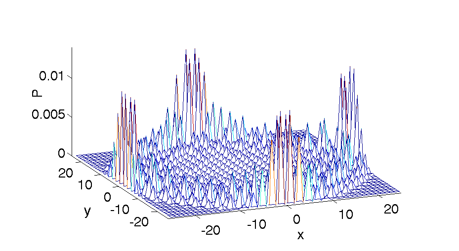
Figure 1: (Color online) Probability distribution for the Grover after 25 steps. An identical distribution using the two-state particle with the $\frac{|0\rangle+i|1\rangle}{\sqrt{2}}$ can be obtained using the alternate walk with the coin operation $B(\pi/4)$ and the Pauli walk after 25 steps.

II.2 Alternate walk

Very recently a 2D quantum walk was suggested which used only a two-state particle which walks first only along the $x$-axis followed by a step along the $y$-axis FGB11 . This walk can results in the same probability distribution as the Grover walk and its evolution is given by

$$|\Psi_{1}\rangle=(\hat{S}_{(0,y)}[\hat{B}(\theta)\otimes\hat{{\mathbbm{1}}}])(\hat{S}_{(x,0)}[\hat{B}(\theta)\otimes\hat{{\mathbbm{1}}}])|\Psi_{\rm in}\rangle,$$ (11)

where

$$\hat{S}_{(x,0)} \equiv \sum_{x,y}\big{[}|0\rangle\langle 0|\otimes|\psi_{x-1,y}\rangle\langle\psi_{x,y}|$$ (12a)

$$\;\;\;\;+|1\rangle\langle 1|\otimes|\psi_{x+1,y}\rangle\langle\psi_{x,y}|\big{]}$$

$$\hat{S}_{(0,y)} \equiv \sum_{x,y}\big{[}|0\rangle\langle 0|\otimes|\psi_{x,y-1}\rangle\langle\psi_{x,y}|$$ (12b)

$$\;\;\;\;+|1\rangle\langle 1|\otimes|\psi_{x,y+1}\rangle\langle\psi_{x,y}|\big{]}.$$

Using a coin operation with $\theta=\pi/4$, the state of the walk after $t$ steps can then be calculated as

$$|\Psi(t)\rangle = \hat{W}(\pi/4)^{t}|\Psi_{\rm in}\rangle$$

$$= \sum_{x=-t}^{t}\sum_{y=-t}^{t}\left[\mathcal{A}_{(x,y),t}|0\rangle+\mathcal{B}_{(x,y),t}|1\rangle\right]\otimes|\psi_{(x,y)}\rangle,$$

where $\hat{W}(\pi/4)=(\hat{S}_{(0,y)}[\hat{B}(\pi/4)\otimes\hat{{\mathbbm{1}}}])(\hat{S}_{(x,0)}[\hat{B}(\pi/4)\otimes\hat{{\mathbbm{1}}}])$, and $\mathcal{A}_{(x,y),t}$ and $\mathcal{B}_{(x,y),t}$ are given by the coupled iterative relations

$$\mathcal{A}_{(x,y),t}=\frac{1}{2}\Big{[} \mathcal{A}_{(x+1,y+1),t-1}+\mathcal{A}_{(x-1,y+1),t-1}$$

$$+\mathcal{B}_{(x+1,y+1),t-1}-\mathcal{B}_{(x-1,y+1),t-1}\Big{]}$$ (14a)

$$\mathcal{B}_{(x,y),t}=\frac{1}{2}\Big{[} \mathcal{A}_{(x+1,y-1),t-1}-\mathcal{A}_{(x-1,y-1),t-1}$$

$$+\mathcal{B}_{(x+1,y-1),t-1}+\mathcal{B}_{(x-1,y-1),t-1}\Big{]}.$$ (14b)

The resulting probability distribution is then

$$P_{2s}=\sum_{x=-t}^{t}\sum_{y=-t}^{t}\left[|\mathcal{A}_{(x,y),t}|^{2}+|\mathcal{B}_{(x,y),t}|^{2}\right],$$ (15)

which for the initial state $|\Psi_{\rm in}\rangle=\frac{1}{\sqrt{2}}(|0\rangle+i|1\rangle)\otimes|\psi_{0,0}\rangle$ gives the same probability distribution as the four-state Grover walk (see Fig. 1).

II.3 Pauli walk

A further scheme to implement a 2D quantum walk using only a two-state particle can be constructed using different Pauli basis states as translational states for the two axis. For convenience we can choose the eigenstates of the Pauli operator $\hat{\sigma}_{3}=\begin{bmatrix}1&~{}~{}0\\ 0&-1\end{bmatrix}$, $|0\rangle$ and $|1\rangle$ as basis states for $x-$axis and eigenstates of $\hat{\sigma}_{1}=\begin{bmatrix}0&1\\ 1&0\end{bmatrix}$, $|+\rangle=\frac{1}{\sqrt{2}}(|0\rangle+|1\rangle)$ and $|-\rangle=\frac{1}{\sqrt{2}}(|0\rangle-|1\rangle)$ as basis states for $y-$axis CBS10 , which also implies that $|0\rangle=\frac{1}{\sqrt{2}}(|+\rangle+|-\rangle)$ and $|1\rangle=\frac{1}{\sqrt{2}}(|+\rangle-|-\rangle)$. In this scheme a coin operation is not necessary and each step of the walk can be implemented by the operation

$$\hat{S}_{\sigma_{3}}\equiv\hat{S}_{(x,0)}$$ (16)

followed by the operation

$$\hat{S}_{\sigma_{1}}\equiv\sum_{x,y}\Big{[} |+\rangle\langle+|\otimes|\psi_{x,y-1}\rangle\langle\psi_{x,y}|$$

$$+|-\rangle\langle-|\otimes|\psi_{x,y+1}\rangle\langle\psi_{x,y}|\Big{]}.$$ (17)

The state after $t$ steps of quantum walk is then given by

$$|\Psi_{t}\rangle = [\hat{S}_{\sigma_{1}}\hat{S}_{\sigma_{3}}]^{t}|\Psi_{\rm in}\rangle$$

$$= \sum_{x=-t}^{t}\sum_{y=-t}^{t}\left[\mathcal{A}_{(x,y),t}|0\rangle+\mathcal{B}_{(x,y),t}|1\rangle\right]\otimes|\psi_{x,y}\rangle,$$

(18)

where $\mathcal{A}_{(x,y),t}$ and $\mathcal{B}_{(x,y),t}$ are given by the coupled iterative relations

$$\mathcal{A}_{(x,y),t}=\frac{1}{2}\Big{[} \mathcal{A}_{(x+1,y+1),t-1}+\mathcal{B}_{(x-1,y+1),t-1}$$

$$+\mathcal{A}_{(x+1,y-1),t-1}-\mathcal{B}_{(x-1,y-1),t-1}\Big{]}$$ (19a)

$$\mathcal{B}_{(x,y),t}=\frac{1}{2}\Big{[} \mathcal{B}_{(x-1,y+1),t-1}+\mathcal{A}_{(x+1,y+1),t-1}$$

$$+\mathcal{B}_{(x-1,y-1),t-1}-\mathcal{A}_{(x+1,y-1),t-1}\Big{]}.$$ (19b)

The probability distribution

$$P_{2s\sigma}=\sum_{x=-t}^{t}\sum_{y=-t}^{t}\left[|\mathcal{A}_{(x,y),t}|^{2}+|\mathcal{B}_{(x,y),t}|^{2}\right]$$ (20)

is again equivalent to the distribution obtained using the Grover walk and therefore also to the alternative walk for the initial state $|\Psi_{\rm in}\rangle=\frac{1}{\sqrt{2}}(|0\rangle+i|1\rangle)\otimes|\psi_{0,0}\rangle$ (see Fig. 1).

While the shift operator for the Grover walk is defined by a single operation, experimentally it has to be implemented as a two shift operations. For example, to shift the state $|0\rangle$ from $(x,y)$ to $(x-1,y-1)$, it has first to be shifted along one axis followed by the other, very similarly to the way it is done in the two-state quantum walk schemes. Therefore, a two-state quantum walk in 2D has many advantages over a four-state quantum walk. The two-state walk using different Pauli basis states for the different axes has the further advantage of not requiring a coin operation at all, making the experimental task even simpler in physical systems where access to different Pauli basis states as translational states is available. One can, of course, also consider including a coin operation in the Pauli walk, which would result in a different probability distributions Cha12 .

For general initial states, quantum walks in 2D with a coin operation $\in U(2)$ can result in a many non-localized probability distribution in position space. This is a further difference to the Grover walk which is very specific with respect to the initial state of the four-state particle and the coin operation.

III Measurement Induced Disturbance

Quantifying non-classical correlations inherent in a certain state is currently one of the most actively studied topics in physics (see for example MBC11 ). While many of the suggested methods involve optimization, making them computationally hard, Luo L08 recently proposed a computable measure that avoids this complication: if one considers a bipartite state $\rho$ living in the Hilbert space ${\cal H}_{A}\otimes{\cal H}_{B}$, one can define a reasonable measure of the total correlations between the systems $A$ and $B$ using the mutual information

$$I(\rho)=S(\rho_{A})+S(\rho_{B})-S(\rho),$$ (21)

where $S(\cdot)$ denotes von Neumann entropy and $\rho_{A}$ and $\rho_{B}$ are the respective reduced density matrices. If $\rho_{A}=\sum_{j}p_{A}^{j}\Pi_{A}^{j}$ and $\rho_{B}=\sum_{j}p_{B}^{j}\Pi_{B}^{j}$, then the measurement induced by the spectral components of the reduced states is

$$\Pi(\rho)\equiv\sum_{j,k}\Pi_{A}^{j}\otimes\Pi_{B}^{k}\rho\Pi_{A}^{j}\otimes\Pi_{B}^{k}.$$ (22)

Given that $I[\Pi(\rho)]$ is a good measure of classical correlations in $\rho$, one may consider a measure for quantum correlations defined by the so-called Measurement Induced Disturbance (MID) L08

$$Q(\rho)=I(\rho)-I[\Pi(\rho)].$$ (23)

MID does not involve any optimization over local measurements and can be seen as a loose upper bound on quantum discord OZ01 . At the same time it is known to capture most of the detailed trends in the behaviour of quantum correlations during quantum walks RSC11 . Therefore, we will use MID ($Q(\rho)$) in the following to quantify quantum correlations for the different 2D quantum walk evolutions.

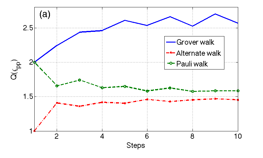
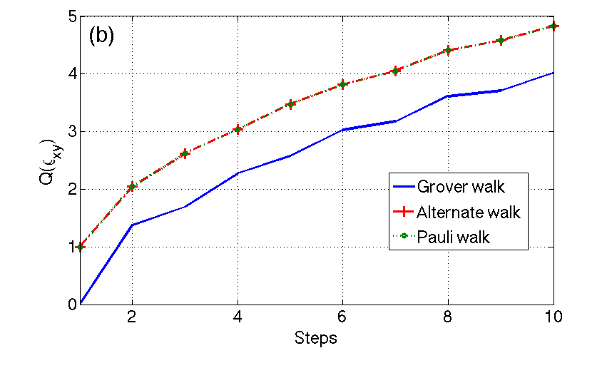
Figure 2: (Color online) Quantum correlations $Q(\rho_{pp})$ and $Q(\rho_{xy})$ for the different schemes in the absence of noise.

Despite having the same probability distributions in the absence of noise, the MIDs for the four-state walk and the two-state walks differ. In Fig. 2(a) we show the MID between the particle and the position degree of freedom, $Q(\rho_{pp})$ for all three walks and find that it is significantly higher for the Grover walk. Where $\rho_{pp}$ is $\tilde{\rho}_{4s}(t)$ for Grover walk, $\tilde{\rho}_{2s}(t)$ for alternate walk and $\tilde{\rho}_{2s\sigma}(t)$ for the Pauli walk. However, due to the difference in the size of the particles degree of freedom for the Grover and the two-state walks, a direct comparison of the quantum correlations $Q(\rho_{pp})$ does not make sense. Among the two-state schemes on the other hand, we see that the Pauli walk has a larger $Q(\rho_{pp})$ in comparison to the alternate walk.

A fair comparison between all systems can be made by looking at the quantum correlations generated between the two spatial dimensions $x$ and $y$, $Q(\rho_{xy})$ (see Fig. 2(b)). $\rho_{xy}$ is obtained by tracing out the particle degree of freedom from from complete density matrix [$\tilde{\rho}_{4s}(t)$, $\tilde{\rho}_{2s}(t)$ and $\tilde{\rho}_{2s\sigma}(t)$] comprising of the particle and the position space. We find that $Q(\rho_{xy})$ is identical for both two-state schemes and exceeding the Grover walk result. This behaviour is similar to the one described in Refs. FGB11 ; FGM11 , where the entanglement created during the Grover walk was compared with the alternate walk using the negativity of the partial transpose, in its generalization for higher-dimensional systems LCO03 ; LKS11 .

IV Decoherence

The effects of noise on 1D quantum walks has been widely studied Ken07 ; CSB07 ; BSC08 ; SBC10 ; RSC11 but the implications in 2D settings are less well known OPD06 ; GAM09 ; Amp12 . In particular no study has been done on either of the two-state schemes presented in the previous section and we therefore now compare their decoherence properties to the Grover walk, using a state-flip and a depolarizing channel as noise models. We show that this leads to differing probability distributions and has an effect on the amounts of quantum correlations as well.

IV.1 State flip noise

IV.1.1 Grover walk

For a two-state particle, state-flip noise simply induces a bit flip [$\sigma_{1}=\begin{bmatrix}0&1\\ 1&0\end{bmatrix}$] but for the Grover walk, the state-flip noise on the four basis states can change one state to 23 other possible permutations. Therefore, the density matrix after $t$ steps in the presence of a state-flip noise channel can be written as

$$\hat{\rho}_{4s}(t) = \frac{p}{k}\left[\sum_{i=1}^{k}\hat{f}_{i}\hat{S}_{4}\hat{\rho}_{4s}(t-1)\hat{S}_{4}{{}^{\dagger}}\hat{f}_{i}{{}^{\dagger}}\right]$$ (24)

$$+(1-p)[\hat{S}_{4}\hat{\rho}_{4s}(t-1)\hat{S}_{4}{{}^{\dagger}}],$$

where $p$ is the noise level, $S_{4}=\hat{S}_{(x,y)}[\hat{G}\otimes\hat{{\mathbbm{1}}}]$, and the $\hat{f}_{i}$ are the state-flip operations.

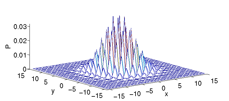
Figure 3: (Color online) Probability distribution of the Grover walk when subjected to a different state-flip noise level with $k=23$ after 15 steps. (a) and (b) are for noise levels, $p=0.1$ and $p=0.9$, respectively.

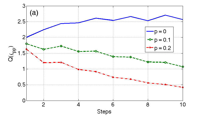
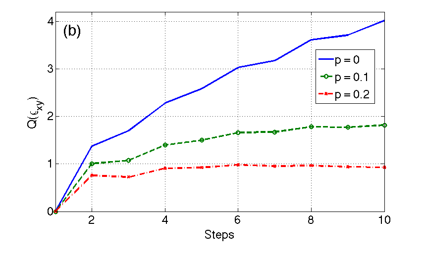
Figure 4: (Color online) Quantum correlations created by the Grover walk in the presence of a noise channel including all possible state flips ($k=23$).

For a noisy channel with all the 23 possible flips one has $k=23$ and in Figs. 3 and 3 we show the probability distribution of the Grover for weak ($p=0.1$) and strong ($p=0.9$) noise levels after 15 step. Compared to the distribution in the absence of noise (see Fig. 1) a progressive reduction in the quantum spread is clearly visible. Note that for $p=1$ the walk corresponds to a fully classical evolution.

In Fig. 4(a) we show the quantum correlations between the particle state with the position space, $Q(\rho_{pp})$, as a function of number of steps $t$. With increasing noise level, a decrease in $Q(\rho_{pp})$ is seen, whereas for the quantum correlations between the $x$ and $y$ spatial dimensions, $Q(\rho_{xy})$, the same amount of noise mainly leads to a decrease in the positive slope (see Fig. 4(b)).

IV.1.2 Two-state walks

The evolution of each step of the two-state quantum walk comprises of a move along one axis followed a move along the other. Therefore, the walk can be subjected to a noise channel after evolution along each axis or after each full step of the walk. In the first case, the noise level $p^{\prime}=\frac{p}{2}$ is applied two times during each step in oder to be equivalent to the application of a noise of strength $p$ in the second case. For the alternate walk the evolution of the density matrix with a bit-flip noise channel applied after evolution along each axis is then given by

$$\hat{\rho}_{2s}^{\prime}(t)= \frac{p}{2}\left[\hat{\sigma}_{1}\hat{S}_{x}\hat{\rho}_{2s}(t-1)\hat{S}_{x}^{\dagger}\hat{\sigma}_{1}^{\dagger}\right]$$

$$+\left(1-\frac{p}{2}\right)\left[\hat{S}_{x}\hat{\rho}_{2s}(t-1)\hat{S}_{x}^{\dagger}\right]$$ (25a)

$$\hat{\rho}_{2s}(t)= \frac{p}{2}\left[\hat{\sigma}_{1}\hat{S}_{y}\hat{\rho}_{2s}^{\prime}(t)\hat{S}_{y}^{\dagger}\hat{\sigma}_{1}^{\dagger}\right]$$

$$+\left(1-\frac{p}{2}\right)\left[\hat{S}_{y}\hat{\rho}_{2s}^{\prime}(t)\hat{S}_{y}^{\dagger}\right],$$ (25b)

where $\hat{\sigma}_{1}=\begin{bmatrix}0&1\\ 1&0\end{bmatrix}\otimes\hat{{\mathbbm{1}}}$, $\hat{S}_{y}=\hat{S}_{(0,y)}[\hat{B}(\theta)\otimes\hat{{\mathbbm{1}}}]$, and $\hat{S}_{x}=\hat{S}_{(x,0)}[\hat{B}(\theta)\otimes\hat{{\mathbbm{1}}}]$.

Similarly, the density matrix with a bit-flip noise applied after the evolution along each axis for the Pauli walk is given by

$$\hat{\rho}_{2s\sigma}^{\prime}(t)= \frac{p}{2}\left[\hat{\sigma}_{1}\hat{S}_{\sigma_{3}}\hat{\rho}_{2s\sigma}(t-1)\hat{S}_{\sigma_{3}}^{\dagger}\hat{\sigma}_{1}^{\dagger}\right]$$

$$+\left(1-\frac{p}{2}\right)\left[\hat{S}_{\sigma_{3}}\hat{\rho}_{2s\sigma}(t-1)\hat{S}_{\sigma_{3}}^{\dagger}\right]$$ (26a)

$$\hat{\rho}_{2s\sigma}(t)= \frac{p}{2}\left[\hat{\sigma}_{1}\hat{S}_{\sigma_{1}}\hat{\rho}_{2s\sigma}^{\prime}(t)\hat{S}_{\sigma_{1}}^{\dagger}\hat{\sigma}_{1}^{\dagger}\right]$$

$$+\left(1-\frac{p}{2}\right)\left[\hat{S}_{\sigma_{1}}\hat{\rho}_{2s\sigma}^{\prime}(t)\hat{S}_{\sigma_{1}}^{\dagger}\right].$$ (26b)

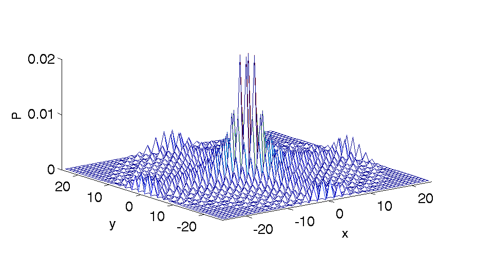
(a) Alternate walk

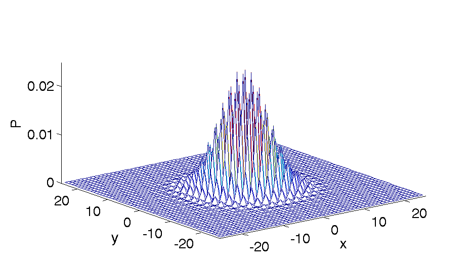
(b) Alternate walk

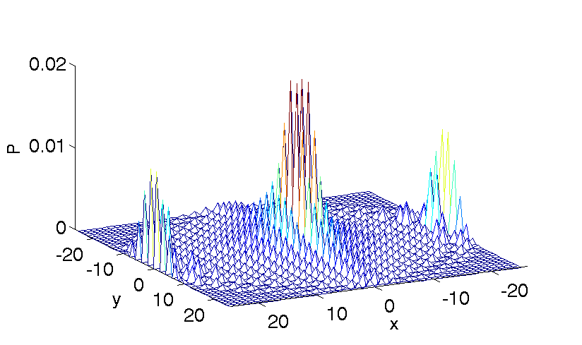
(c) Pauli walk

(d) Pauli walk

Figure 5: (Color online) Probability distributions of the two-state walk with the bit-flip noise applied after evolution in each direction. The strength of the noise is $p/2=0.05$ in (a) and (c) and $p/2=0.45$ in (c) and (d) and the evolution was carried out for 25 step each time.

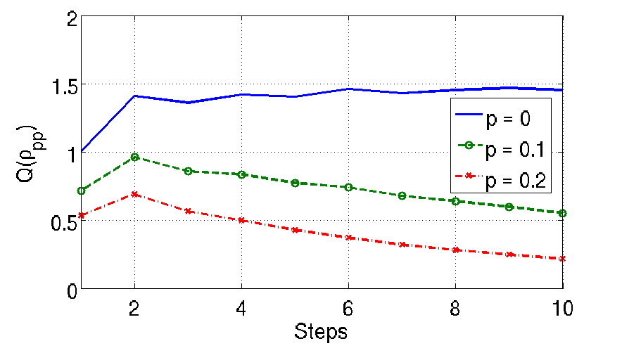
(a) Alternate walk

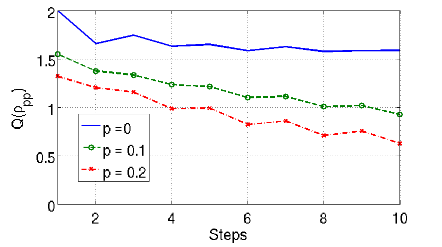
(b) Pauli Walk

Figure 6: (Color online) Particle-position quantum correlations created by the two-state walks for different bit-flip noise levels applied after evolution along each axis.

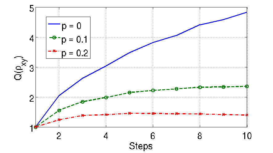
(a) Alternate walk

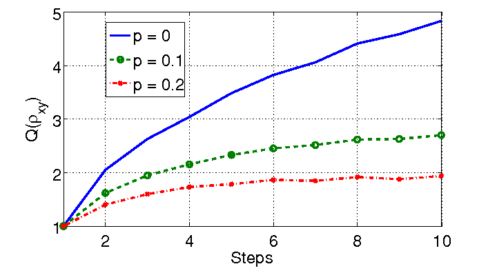
(b) Pauli walk

Figure 7: (Color online) Quantum correlations between the $x$ and $y$ spatial dimensions created by the two-state walks for different bit-flip noise levels applied after evolution along each axis

In Figs. 5(a) and 5(b) the probability distributions for the alternate walk after 25 steps of noisy evolution with $p=0.1$ and $p=0.9$ are shown and Figs. 5(c) and 5(d) show the same for the Pauli walk. It can be seen that the bit-flip noise channel acts symmetrically on both axes for the alternate walk, but asymmetrically on the Pauli walk. This is due to the fact that the bit-flip noise applied along the axis in which the $\sigma_{1}$ Pauli basis is used leaves the state unchanged. A completely classical evolution is recovered for $p=1$ ($p^{\prime}=0.5$) and an evolution with $p=2$ is equivalent to one with $p=0$.

Evolving the density matrix and calculating the MID for a noiseless evolution ($p=0$), one can see from Fig. 6 that the initial difference in $Q(\rho_{pp})$ between the Pauli walk and the alternate walk decreases during the evolution and eventually both values settle around 1.5. For a noisy evolution, however, the initial difference in $Q(\rho_{pp})$ does not decrease over time and we find a higher value for the Pauli walk compared to the alternate walk. Similarly, careful examination of Fig. 7 shows that the $Q(\rho_{xy})$ for the alternate walk and the Pauli walk are identical in the absence of noise, but differ for noisy evolution, with the alternate walk being affected stronger than the Pauli walk.

The density matrix for the second case, that is, with a noisy channel applied only once after one full step of walk evolution, for both two-state walks is given by

$$\hat{\rho}_{2s}(t) =p\left[\hat{\sigma}_{1}\hat{Q}(t-1)\hat{\sigma}_{1}^{\dagger}\right]+(1-p)\hat{Q}(t-1)$$ (27a)

$$\hat{\rho}_{2s\sigma}(t) =p\left[\hat{\sigma}_{1}\hat{Q}_{\sigma}(t-1)\hat{\sigma}_{1}^{\dagger}\right]+(1-p)\hat{Q}_{\sigma}(t-1)$$ (27b)

where

$$\hat{Q}(t-1) =\hat{S}_{y}\hat{S}_{x}\hat{\rho}_{2s}(t-1)\hat{S}_{x}^{\dagger}\hat{S}_{y}^{\dagger}$$ (28a)

$$\hat{Q}_{\sigma}(t-1) =\hat{S}_{\sigma_{1}}\hat{S}_{\sigma_{3}}\hat{\rho}_{2s\sigma}(t-1)\hat{S}_{\sigma_{3}}^{\dagger}\hat{S}_{\sigma_{1}}^{\dagger}.$$ (28b)

In this case maximum decoherence and a completely classical evolution is obtained for $p=0.5$ and the evolution with $p=1$ is equivalent to the one with $p=0$. The obtained probability distributions are almost identical for both walks and differ only slightly from the ones obtained for the alternate walk with noise applied after evolution along each axis (see Fig. 5(a) and 5(b)). The correlation functions $Q(\rho_{pp})$ and $Q(\rho_{xy})$ behave very similar for both walks (see Figs. 8 and 9) and we can conclude that the presence of bit-flip noise on both two-state walks when applied after a full step leads to equally strong decoherence.

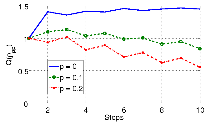
(a) Alternate walk

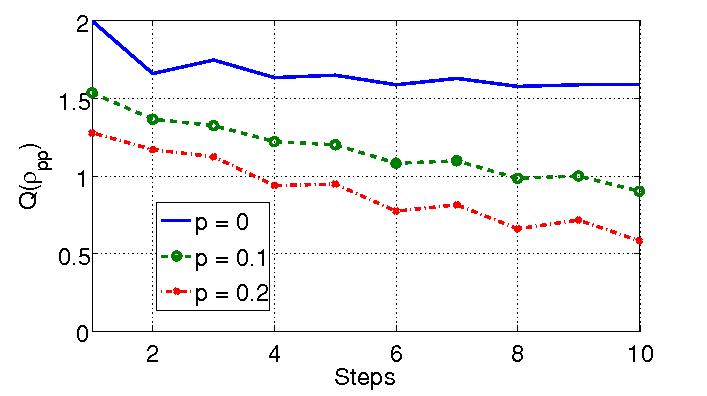
(b) Pauli walk

Figure 8: (Color online) Particle-position quantum correlations created by the two-state walks for different bit-flip noise levels applied after evolution of one complete step.

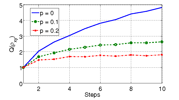
(a) Alternate walk

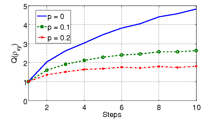
(b) Pauli walk

Figure 9: (Color online) Quantum correlations between the $x$ and $y$ spatial dimensions created by the two-state walks for different bit-flip noise levels applied after evolution of one complete step.

IV.2 Depolarizing channel

To describe depolarizing noise we use the standard model in which the density matrix of our two-state system is replaced by a linear combination of a completely mixed and an unchanged state,

$$\hat{\rho}=\frac{p}{3}\left(\hat{\sigma}_{1}\hat{\rho}\hat{\sigma}_{1}+\hat{\sigma}_{2}\hat{\rho}\hat{\sigma}_{2}+\hat{\sigma}_{3}\hat{\rho}\hat{\sigma}_{3}\right)+(1-p)\hat{\rho},$$ (29)

where $\hat{\sigma}_{1}$, $\hat{\sigma}_{2}$ and $\hat{\sigma}_{3}$ are the standard Pauli operators. To be able to compare the effects of the depolarizing channel on the Grover walk and the two-state walks we will apply the noise only once after each full step.

IV.2.1 Grover walk

For the four-state particle the depolarizing noise channel comprises of all possible state flips, phase flips and their combinations. State-flip noise alone leads to 23 possible changes in the four-state system and adding the phase-flip noise and all combinations of these two is unfortunately a task beyond current computational ability. Therefore let us first briefly investigate the possibility of approximating the state flip noise by restricting ourselves to only a subset of flips. One example would be a noisy channel with only 6 possible flips ($k=6$) between two of the four basis states

$$\hat{f}_{1}=\begin{bmatrix}0&1&0&0\\ 1&0&0&0\\ 0&0&1&0\\ 0&0&0&1\end{bmatrix}\otimes\hat{{\mathbbm{1}}}~{}~{};~{}~{}\hat{f}_{2}=\begin{bmatrix}0&0&1&0\\ 0&1&0&0\\ 1&0&0&0\\ 0&0&0&1\end{bmatrix}\otimes\hat{\mathbbm{1}}$$

$$\hat{f}_{3}=\begin{bmatrix}0&0&0&1\\ 0&1&0&0\\ 0&0&1&0\\ 1&0&0&0\end{bmatrix}\otimes\hat{\mathbbm{1}}~{}~{};~{}~{}\hat{f}_{4}=\begin{bmatrix}1&0&0&0\\ 0&0&1&0\\ 0&1&0&0\\ 0&0&0&1\end{bmatrix}\otimes\hat{\mathbbm{1}}$$

$$\hat{f}_{5}=\begin{bmatrix}1&0&0&0\\ 0&0&0&1\\ 0&0&1&0\\ 0&1&0&0\end{bmatrix}\otimes\hat{\mathbbm{1}}~{}~{};~{}~{}\hat{f}_{6}=\begin{bmatrix}1&0&0&0\\ 0&1&0&0\\ 0&0&0&1\\ 0&0&1&0\end{bmatrix}\otimes\hat{\mathbbm{1}}$$ (30)

and another a channel where only cyclic flips ($k=3$) of all the basis states can appear

$$\hat{f}_{1}=\hat{f}\otimes\hat{{\mathbbm{1}}}~{}~{};~{}~{}\hat{f}_{2}=\hat{f}^{2}\otimes\hat{{\mathbbm{1}}}~{}~{};~{}~{}\hat{f}_{3}=\hat{f}^{3}\otimes\hat{{\mathbbm{1}}}$$ (31)

with $\hat{f}=\begin{bmatrix}0&1&0&0\\ 0&0&1&0\\ 0&0&0&1\\ 1&0&0&0\end{bmatrix}$. The probability distributions for these two approximations are visually very similar to the situation where all possible state-flips are taken into account ($k=23$) and in Fig. 10 we compare the results obtained for the the $x-y$ spatial quantum correlations for a noise level of $p=0.1$.

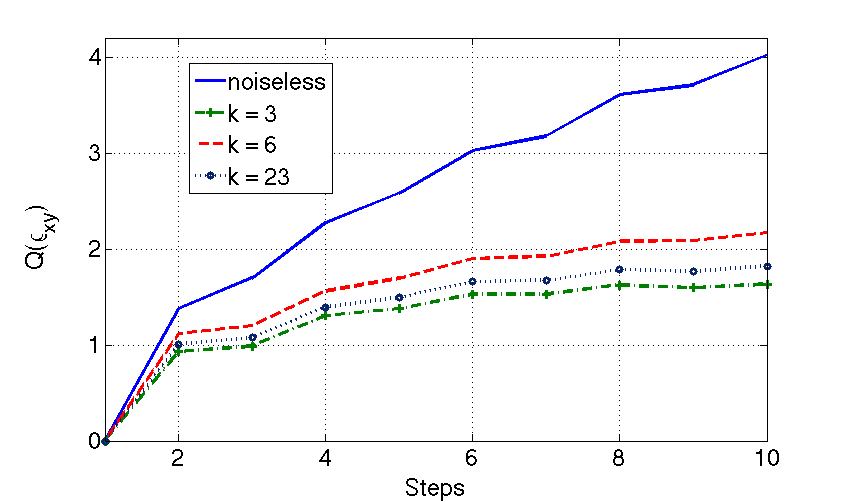
Figure 10: (Color online) Quantum correlations between the $x$ and $y$ spatial dimensions for the Grover walk in the presence of a state-flip noise channel with $p=0.1$. The noise is modelled as state-flips including all possible flips ($k=23$), flips between only two of the basis states ($k=6$) and cyclic flips of all the four basis state ($k=3$)

One can see that the spatial quantum correlations are affected stronger by the $k=3$ than by the full $k=23$ flip noise. This implies that the two- and three state flips included in $k=23$ acts as reversals of cyclic flips, thereby reducing the effect of noise. Since the trends for the decrease of the quantum correlation are functionally similar for $k=3,6$ and 23, we will use the model with $k=3$ cyclic flips as the state-flip noise channel for the Grover walk in this section. Similarly, taking into account the computational limitations and following the model adopted for the state-flip, we will use a cyclic phase-flips to model the phase-flip noise,

$$\hat{r}_{1}=\hat{r}\otimes\hat{\mathbbm{1}}~{}~{};~{}~{}\hat{r}_{2}=\hat{r}^{2}\otimes\hat{\mathbbm{1}}~{}~{};~{}~{}\hat{r}_{3}=\hat{r}^{3}\otimes\hat{\mathbbm{1}},$$ (32)

where $\hat{r}=\begin{bmatrix}1&0&0&0\\ 0&\omega&0&0\\ 0&0&\omega^{2}&0\\ 0&0&0&\omega^{3}\end{bmatrix}$ with $\omega=e^{\frac{2\pi i}{4}}$.

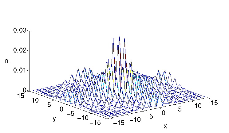
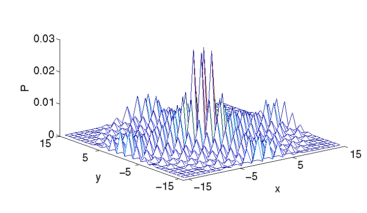
Figure 11: (Color online) Probability distribution of (a) the Grover walk and (b) the two-state walks when subjected to a depolarizing channel. For the Grover walk the channel is given by Eq. (33) and for all walks the noise level is $p=0.1$. The distribution is shown after 15 steps of evolution.

Both these approximations for state-flip and phase-flip noise will makes the complex depolarization noise manageable for numerically treatment. The density matrix of the Grover walk can then be written as

$$\hat{\rho}_{4s}(t) = \frac{p}{15}\left[\sum_{i=1}^{3}\hat{f}_{i}\hat{S}_{4}\hat{\rho}_{4s}(t-1)\hat{S}_{4}{{}^{\dagger}}\hat{f}_{i}{{}^{\dagger}}\right]$$ (33)

$$+ \frac{p}{15}\left[\sum_{j=1}^{3}\hat{r}_{j}\hat{S}_{4}\hat{\rho}_{4s}(t-1)\hat{S}_{4}{{}^{\dagger}}\hat{r}_{j}{{}^{\dagger}}\right]$$

$$+ \frac{p}{15}\left[\sum_{i=1}^{3}\sum_{j=1}^{3}\hat{r}_{j}\hat{f}_{i}\hat{S}_{4}\hat{\rho}_{4s}(t-1)\hat{S}_{4}{{}^{\dagger}}\hat{f}_{i}^{\dagger}\hat{r}_{j}{{}^{\dagger}}\right]$$

$$+(1-p)[\hat{S}_{4}\hat{\rho}_{4s}(t-1)\hat{S}_{4}{{}^{\dagger}}]$$

and the probability distribution for this walk is shown in Fig. 11 for $p=0.1$. The quantum correlations $Q(\rho_{pp})$ and $Q(\rho_{xy})$ are shown in Fig. 12. With increasing noise level, a decrease in $Q(\rho_{pp})$ is seen, whereas for the quantum correlations between the $x$ and $y$ spatial dimensions, $Q(\rho_{xy})$, the same amount of noise mainly leads to a decrease in the positive slope (see Fig. 12). From this we can conclude that the general trend in the quantum correlaltion due to state-flip noise (Fig. 4) and depolarizing noise is the same but the effect is slightly stronger when including the depolarizing channel.

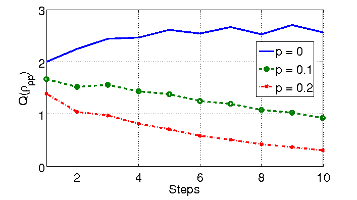
(a) Grover walk

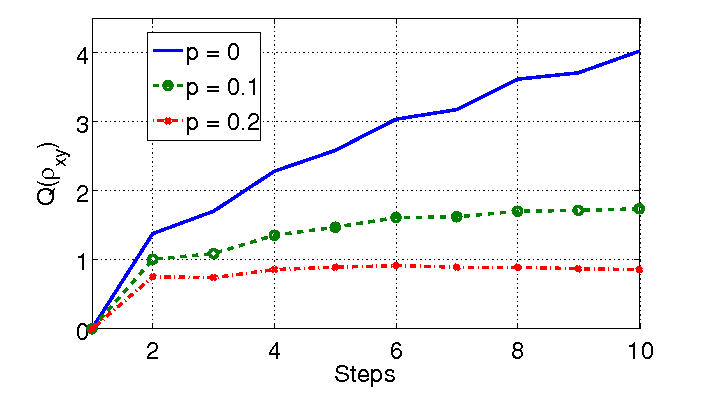
(b) Grover walk

Figure 12: (Color online) Quantum correlations created by the Grover walk for different depolarizing noise levels.

IV.2.2 Two-state walks

The depolarizing channels for the alternate walk and Pauli walk can be written as

$$\hat{\rho}_{2s}(t) =\frac{p}{3}\left[\sum_{i=1}^{3}\hat{\sigma}_{i}\hat{Q}(t-1)\hat{\sigma}_{i}^{\dagger}\right]+(1-p)\hat{Q}(t-1)$$ (34a)

$$\hat{\rho}_{2s\sigma}(t) =\frac{p}{3}\left[\sum_{i=1}^{3}\hat{\sigma}_{i}\hat{Q}_{\sigma}(t-1)\hat{\sigma}_{i}^{\dagger}\right]+(1-p)\hat{Q}_{\sigma}(t-1),$$ (34b)

where $\hat{\sigma}_{1}=\begin{bmatrix}0&1\\ 1&0\end{bmatrix}\otimes\hat{{\mathbbm{1}}}$, $\hat{\sigma}_{2}=\begin{bmatrix}0&-i\\ i&~{}~{}0\end{bmatrix}\otimes\hat{{\mathbbm{1}}}$, $\hat{\sigma}_{3}=\begin{bmatrix}1&~{}~{}0\\ 0&-1\end{bmatrix}\otimes\hat{{\mathbbm{1}}}$ and $\hat{Q}(t-1)$ and $\hat{Q}_{\sigma}(t-1)$ are given by Eqs. (28a) and (28b).

Similarly to the situation where we considered only state-flip noise after one complete step (see Figs. 8 and 9) we find again that the quantum correlations for both walks behave nearly identical and only differ slightly in strength compared to the case of state-flip noise alone (see Figs. 13 and 14).

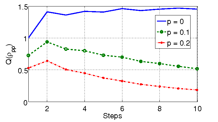
(a) Alternate walk

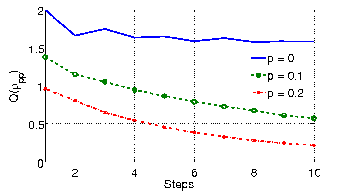
(b) Pauli walk

Figure 13: (Color online) Particle-position quantum correlations created by the two-state walks for different depolarizing noise levels.

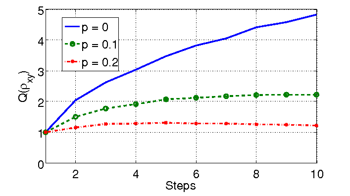
(a) Alternate walk

(b) Pauli walk

Figure 14: (Color online) Quantum correlations between the $x$ and $y$ spatial dimensions created by the two-state walks for different depolarizing noise levels.

IV.3 Robustness of two-state walk

From the preceding sections we note that the $x-y$ spatial correlations, $Q(\rho_{xy})$, have a larger absolute value for the two-state walks compared to the Grover walk and that the presence of noise affects all schemes in a similar manner. To quantify and better illustrate the effect the noise has we therefore calculate

$$R(\rho_{xy})=\frac{Q(\rho_{xy})\quad\text{for noisy walk}}{Q(\rho_{xy})\quad\text{for noiseless walk}},$$ (35)

as a function of number of steps, which gives the rate of decrease in the quantum correlations. In Figs. 15 and 16 we show this quantity in the presence of state-flip or depolarizing noise, respectively, for a noise level of $p=0.2$. One can clearly see that in both cases the two-state walks are more robust against the noise at any point during the evolution. Note that the Grover walk only produces correlations from step 2 on, which is the reason for its graph starting later.

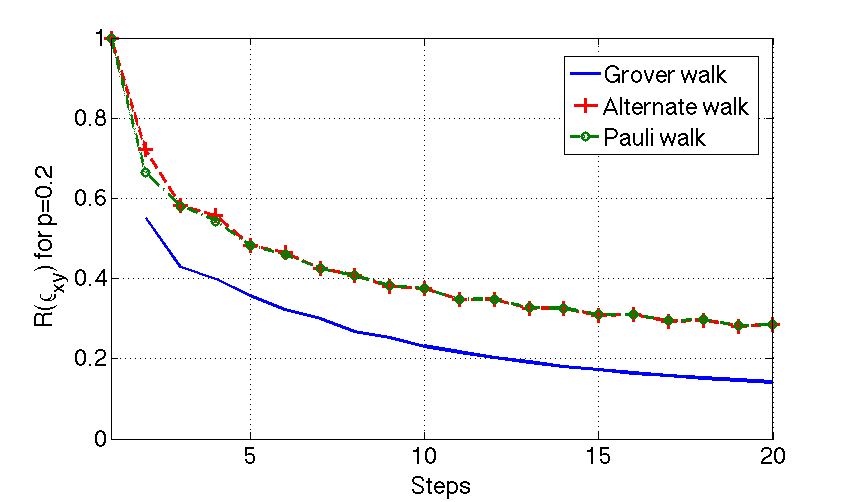
Figure 15: (Color online) Relative decay of the quantum correlations $Q(\rho_{xy})$ in the presence of a state-flip noise channel with $p=0.2$.

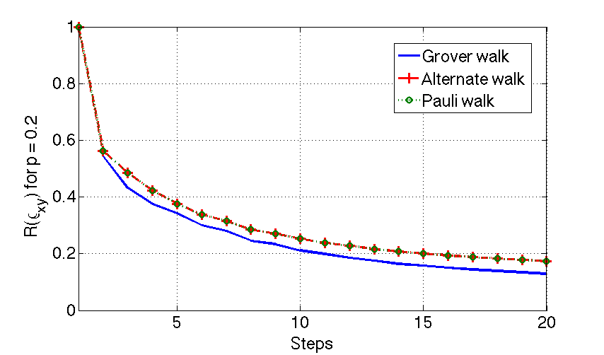
Figure 16: (Color online) Relative decay of the quantum correlations $Q(\rho_{xy})$ in the presence of a depolarizing noise channel with $p=0.2$.

V Breakdown of state-flip and phase-flip symmetries for four-state walks

The quantum walk of a two-state particle in 1D is known to remain unaltered in the presence of unitary operations which equally effect each step of the evolution. This is due to the existence of symmetries CSB07 ; BSC08 , which can help to identify different variants of the same quantum walk protocol and which can be useful in designing experimental implementation. For example, in a recent scheme used to implement a one-dimensional quantum walk using atoms in an optical lattice Cha06 , the conditional shift operator also flipped the state of the atom with every shift in position space. However, the existence of a bit-flip symmetry in the system allowed to implement the walk without the need for compensation of these bit-flips. In this section we look at possible symmetries in the walks discussed above and show that the bit-flip and phase-flip symmetries, which are present in the evolution of the two-state particle are absent in the evolution of the four-state particle.

The density matrix for a two-state quantum walk in the presence of a noisy channel will evolve through a linear combination of noisy operations on the state and the unaffected state itself. As an example we illustrate the symmetry due to bit-flip operations in the alternate walk with bit-flip noise after evolution of one complete step. The density matrix in this case is given by

$$\hat{\rho}_{2s}(t) = p\Big{[}\hat{\sigma}_{1}\hat{S}_{y}\hat{S}_{x}\hat{\rho}_{2s}(t-1)\hat{S}_{x}^{\dagger}\hat{S}_{y}^{\dagger}\hat{\sigma}^{\dagger}_{1}\Big{]}$$ (36)

$$+(1-p)\Big{[}\hat{S}_{y}\hat{S}_{x}\hat{\rho}_{2s}(t-1)\hat{S}^{\dagger}_{x}\hat{S}^{\dagger}_{y}\Big{]},$$

where $\hat{\sigma_{1}}=\begin{bmatrix}0&1\\ 1&0\end{bmatrix}\otimes\hat{{\mathbbm{1}}}$. When the noise level is $p=1$ this expression reduces to

$$\hat{\rho}_{2s}(t) = \Big{[}\hat{\sigma}_{1}\hat{S}_{y}\hat{S}_{x}\hat{\rho}_{2s}(t-1)\hat{S}_{x}^{\dagger}\hat{S}_{y}^{\dagger}\hat{\sigma}^{\dagger}_{1}\Big{]}$$ (37)

$$= \hat{S}^{\prime}_{y}\hat{S}_{x}\hat{\rho}_{2s}(t-1)\hat{S}_{x}^{\dagger}(\hat{S}_{y}^{\prime})^{\dagger}.$$

where in the second line the bit-flip operation has been absorbed into the evolution operator $\hat{S}^{\prime}_{y}$. This replaces $|0\rangle\langle 0|$ and $|1\rangle\langle 1|$ in $\hat{S}_{y}$ by $|1\rangle\langle 0|$ and $|0\rangle\langle 1|$, respectively. Similarly, for a phase-flip, $\hat{\sigma_{1}}$ in Eq. (37) is replaced by $\hat{\sigma_{3}}=\begin{bmatrix}1&0\\ 0&-1\end{bmatrix}\otimes\hat{{\mathbbm{1}}}$ leading to $|1\rangle\langle 1|$ in $\hat{S}_{y}$ being replaced by $-|1\rangle\langle 1|$ to construct $\hat{S}^{\prime}_{y}$.

An alternative way to look at this is to absorb the bit-flip or phase-flip operation into the coin operation. For a two-state walk using the Hadamard coin operation, the bit-flip operation after each steps corresponds to the coin operation taking the form,

$$\hat{H}^{\prime}=\frac{1}{\sqrt{2}}\begin{bmatrix}1&&-1\\ 1&&~{}~{}1\end{bmatrix}$$ (38)

and the phase-flip after each steps corresponds to the coin operation taking the form,

$$\hat{H}^{\prime\prime}=\frac{1}{\sqrt{2}}\begin{bmatrix}~{}~{}1&&1\\ -1&&1\end{bmatrix}.$$ (39)

For a bit-flip or phase-flip of noise level $p=1$ the Hadamard coin operation $\hat{H}$ can therefore be recast into a noiseless ($p=0$) quantum walk evolution using $\hat{H}^{\prime}$ and $\hat{H}^{\prime\prime}$ as coin operation. A noise level of $p=1$ then returns a probability distribution equivalent to the noiseless evolution and consequently the maximum bit-flip and phase-flip noise level for a two state walk corresponds to $p=0.5$. This is a symmetry within the alternate walk, which also holds for the Pauli walk.

A state-flip noise channel for the four-state walk, on the other hand, evolves the state into a linear combination of all possible flips between the four basis states and an unchanged state for all values of $p$ except for $p=0$ (see Eq. 24). That is, only when $p=0$, Eq. (24) reduces to

$$\hat{\rho}_{4s}(t)=\hat{S}_{4}\hat{\rho}_{4s}(t-1)\hat{S}_{4}{{}^{\dagger}},$$ (40)

whereas for any non-zero $p$ including $p=1$, Eq. (24) takes the form

$$\hat{\rho}_{4s}(t) = \frac{1}{k}\left[\sum_{i=1}^{k}\hat{f}_{i}\hat{S}_{4}\hat{\rho}_{4s}(t-1)\hat{S}_{4}{{}^{\dagger}}\hat{f}_{i}{{}^{\dagger}}\right],$$ (41)

Any attempt to absorb the noise operations $\hat{f}_{i}$ into the shift operator or the coin operation leads to $k$ different results, which have to be applied with probability $\frac{1}{k}$. Therefore, in contrast to the two-state evolution, a state flip noise level of $p=1$ does not result in a pure evolution equivalent to the situation for $p=0$. However, if the state-flip noise is restricted to one possible operation ($\hat{f}_{i}$), the density matrix is no longer a linear combination of noisy operations and the unchanged state. Thus, for $p=1$ in Eq. (24) a single noise operation can be absorbed into the GDO by changing the form of $G$ (see Eq. (5)).

This absence of a useful symmetry for the four-state quantum walk reduces the chances to find an equivalent class of four-state quantum walk evolutions. Furthermore, since the four-state quantum walk requires a specific form of coin operation to implement the walk, any possible absorption will not result in a quantum walk in 2D, which is a significant difference to the two-state walks.

VI Conclusion

In this work we have studied the decoherence properties of three different schemes that realize a quantum walk in two-dimensions, namely the Grover (four-state) walk, the alternate walk and the Pauli walk. The noise for two-state particle evolution was modeled using a bit-flip channel and depolarizing channel. For the four-state evolution, different possible state-flip channels were explored and we have shown a channel with 3 cyclic flips between all the four states can be used as a very good approximation to the full situation. Similarly, we presented a possible model for the depolarizing channel of the four-state quantum walk. Using MID as a measure for the quantum correlations within the state, our studies have shown that the two-state quantum walk evolution is in general more robust against decoherence from state-flip and depolarizing noise channels.

Following earlier studies on bit- and phase-flip symmetries in two-state quantum walks in 1D, we have shown that they also hold for two-state quantum walks in 2D, but break down for four-state 2D quantum walks.

With the larger robustness against decoherence, the existence of symmetries which allow freedom of choice with respect to the initial state and the coin operation and the much easier experimental control, we conclude that two-state particles can be conveniently used to implement quantum walks in 2D compared to schemes using higher dimensional coins. An other important point to be noted is the straightforward extendability of the both two-state schemes to higher dimensions by successively carrying out the evolution in each dimension.

Acknowledgement: We acknowledge support from Science Foundation Ireland under Grant No. 10/IN.1/I2979. We would like to thank Carlo Di Franco and Gianluca Giorgi for helpful discussions.

References

- (1) G. V. Riazanov, Sov. Phys. JETP 6 1107 (1958).
- (2) R. Feynman, Found. Phys. 16, 507 (1986).
- (3) K. R. Parthasarathy, Journal of Applied Probability, 25, 151-166 (1988).
- (4) J. M. Lindsay and K. R. Parthasarathy, Sankhy: The Indian Journal of Statistics, Series A, 50, 151-170 (1988).
- (5) Y. Aharonov, L. Davidovich and N. Zagury, Phys. Rev. A 48, 1687, (1993).
- (6) J. Kempe, Contemp. Phys. 44, 307 (2003).
- (7) A. Ambainis, Int. Journal of Quantum Information, 1, No.4, 507-518 (2003).
- (8) G. S. Engel, T. R. Calhoun, E. L. Read, T. Ahn, T. Manal, Y. Cheng, R. E. Blankenship, and G. R. Fleming, Nature 446, 782-786 (2007).
- (9) M. Mohseni, P. Rebentrost, S. Lloyd, A. Aspuru-Guzik, J. Chem. Phys. 129, 174106 (2008).
- (10) C. M. Chandrashekar and R. Laflamme, Phys. Rev. A 78, 022314 (2008).
- (11) C. M. Chandrashekar, Phys. Rev. A, 83, 022320 (2011).
- (12) T. Kitagawa, M. S. Rudner, E. Berg, and E. Demler, Phys. Rev. A 82, 033429 (2010).
- (13) S. K. Goyal, C. M. Chandrashekar, J. Phys. A: Math. Theor. 43, 235303 (2010).
- (14) J. Du, H. Li, X. Xu, M. Shi, J. Wu, X. Zhou, and R. Han, Phys. Rev. A 67, 042316 (2003).
- (15) C. A. Ryan, M. Laforest, J. C. Boileau, and R. Laflamme, Phys. Rev. A 72, 062317 (2005).
- (16) D. Lu, J. Zhu, P. Zou, X. Peng, Y. Yu, S. Zhang, Q. Chen, and J. Du, Phys. Rev. A 81, 022308 (2010).
- (17) H. Schmitz, R. Matjeschk, Ch. Schneider, J. Glueckert, M. Enderlein, T. Huber, and T. Schaetz, Phys. Rev. Lett. 103, 090504 (2009).
- (18) F. Zahringer, G. Kirchmair, R. Gerritsma, E. Solano, R. Blatt, and C. F. Roos, Phys. Rev. Lett. 104, 100503 (2010).
- (19) H. B. Perets, Y. Lahini, F. Pozzi, M. Sorel, R. Morandotti, and Y. Silberberg, Phys. Rev. Lett. 100, 170506 (2008).
- (20) A. Schreiber, K. N. Cassemiro, V. Potocek, A. Gabris, P. Mosley, E. Andersson, I. Jex, and Ch. Silberhorn, Phys. Rev. Lett., 104, 050502 (2010).
- (21) M. A. Broome, A. Fedrizzi, B. P. Lanyon, I. Kassal, A. Aspuru-Guzik, and A. G. White. Phys. Rev. Lett. 104, 153602 (2010).
- (22) A. Peruzzo, M. Lobino, J. C. F. Matthews, N. Matsuda, A. Politi, K. Poulios, X. Zhou, Y. Lahini, N. Ismail, K. Wörhoff, Y. Bromberg, Y. Silberberg, M. G. Thompson, and J. L. OBrien, Science 329, 1500 (2010).
- (23) A. Schreiber, K. N. Cassemiro, V. Potocek, A. Gabris, I. Jex, and Ch. Silberhorn, Phys. Rev. Lett. 106, 180403 (2011).
- (24) L. Sansoni, F. Sciarrino, G. Vallone, P. Mataloni, A. Crespi, R. Ramponi, and R. Osellame Phys. Rev. Lett. 108, 010502 (2012).
- (25) K. Karski, L. Foster, J.-M. Choi, A. Steffen, W. Alt, D. Meschede, and A. Widera, Science 325, 174 (2009).
- (26) E. Farhi and S. Gutmann, Phys.Rev. A 58, 915 (1998).
- (27) D. A. Meyer, J. Stat. Phys. 85, 551 (1996).
- (28) A. Ambainis, E. Bach, A. Nayak, A. Vishwanath and J. Watrous, Proceeding of the 33rd ACM Symposium on Theory of Computing (ACM Press, New York, 2001), p.60.
- (29) A. Nayak and A. Vishwanath, DIMACS Technical Report, No. 2000-43 (2001).
- (30) N. Konno, Quantum Information Processing, Vol.1, pp.345-354 (2002).
- (31) E. Bach, S. Coppersmith, M. P. Goldschen, R. Joynt, and J. Watrous, J. Comput. Syst. Sci., 69, 562 (2004).
- (32) C. M. Chandrashekar, R. Srikanth, and R. Laflamme, Phys. Rev. A 77, 032326 (2008).
- (33) T. D. Mackay, S. D. Bartlett, L. T. Stephenson, B. C. Sanders, J. Phys. A: Math. Gen. 35, 2745 (2002).
- (34) B. Tregenna, W. Flanagan, R. Maile, and V. Kendon, New Journal of Physics 5, 83 (2003).
- (35) C. S. Hamilton , A. Gabris , I. Jex, and S. M. Barnett, New Journal of Physics 13, 013015 (2011).
- (36) K. Eckert, J. Mompart, G. Birkl, and M. Lewenstein, Phys. Rev. A 72, 012327 (2005).
- (37) A. C. Oliveira and R. Portugal, and R. Donangelo, Phys. Rev. A 74, 012312 (2006).
- (38) C. Di Franco, M. Mc Gettrick, and Th. Busch, Phys. Rev. Lett. 106, 080502 (2011).
- (39) C. Di Franco, M. Mc Gettrick, T. Machida, and Th. Busch, Phys. Rev. A 84, 042337 (2011).
- (40) C. M. Chandrashekar, S. Banerjee, and R. Srikanth, Phys. Rev. A 81, 062340 (2010).
- (41) C.M. Chandrashekar, arXiv:1103.2704 (2011).
- (42) S. Luo, Phys. Rev. A 77 022301 (2008).
- (43) N. Inui, Y. Konishi, and N. Konno, Phys. Rev. A 69, 052323 (2004).
- (44) M. Stefanak, T. Kiss, and I. Jex, Phys. Rev. A 78, 032306 (2008).
- (45) K. Modi, A. Brodutch, H. Cable, T. Paterek, and V Vedral, arXiv:1112.6238.
- (46) H. Ollivier and W. H. Zurek , Phys. Rev. Lett. 88, 017901 (2001).
- (47) B. R. Rao, R. Srikanth, C. M. Chandrashekar and S. Banerjee, Phys. Rev. A, 83, 064302 (2011).
- (48) S. Lee, D. Chi, S. Oh, and J. Kim, Phys. Rev. A 68, 062304 (2003).
- (49) S. Lee, J. S. Kim, and B. C. Sanders, Phys. Lett. A 375, 411-414 (2011).
- (50) R. Srikanth, S. Banerjee, and C. M. Chandrashekar, Phys. Rev. A, 81, 062123 (2010).
- (51) V. Kendon, Math. Struct. Computer Science 17, 1169 (2007).
- (52) C. M. Chandrashekar, R. Srikanth, and S. Banerjee, Phys. Rev. A, 76, 022316 (2007).
- (53) S. Banerjee, R. Srikanth, C. M. Chandrashekar, and P. Rungta, Phys. Rev. A, 78, 052316 (2008).
- (54) M. Gonulol, E. Aydiner, O. E. Mustecaplioglu, Phys. Rev. A 80, 022336 (2009).
- (55) C. Ampadu, Communications in Theoretical Physics, 57, Number 1, pp 41-55 (2012).
- (56) C. M. Chandrashekar, Phys. Rev. A 74, 032307 (2006).