Suppressing nano-scale stick-slip motion by feedback

Abstract

When a micro cantilever with a nano-scale tip is manipulated on a substrate with atomic-scale roughness, the periodic lateral frictional force and stochastic fluctuations may induce stick-slip motion of the cantilever tip, which greatly decreases the precision of the nano manipulation. This unwanted motion cannot be reduced by open-loop control especially when there exist parameter uncertainties in the system model, and thus needs to introduce feedback control. However, real-time feedback cannot be realized by the existing virtual reality virtual feedback techniques based on the position sensing capacity of the atomic force microscopy (AFM). To solve this problem, we propose a new method to design real-time feedback control based on the force sensing approach to compensate for the disturbances and thus reduce the stick-slip motion of the cantilever tip. Theoretical analysis and numerical simulations show that the controlled motion of the cantilever tip tracks the desired trajectory with much higher precision. Further investigation shows that our proposal is robust under various parameter uncertainties. Our study opens up new perspectives of real-time nano manipulation.

I Introduction

One of the central problems in nano science and technology Feynman is the realization of high-precision nano manipulation, e.g., pushing, pulling, rotating, rolling, and cutting nano-scale objects. In the widely applied AFM experiments Binnig1 ; Binnig2 ; Junno ; Martin ; Guthold ; Sitti1 ; Sitti2 ; XiNing1 ; XiNing2 ; TianXiaoJun ; LiuLianQing ; ZhangYu , a large amount of frontier progresses have been achieved about nano manipulation. However, the theoretical analysis for such system is mainly focused on the static force analysis within a Newton-mechanical framework Junno ; Martin ; Guthold ; Sitti1 ; Sitti2 ; XiNing1 ; XiNing2 ; TianXiaoJun ; LiuLianQing ; ZhangYu that describes the macroscopic system. Recent experiments show that the force analysis in the nano scale is not the same as that at the macroscopic scale. Typically, nano-scale friction PerssonBook ; PerssonRMP is logarithmically dependent on the velocity Gnecco ; Riedo ; Tambe , which is quite different from the macroscopic sliding friction (the friction is independent on the velocity) and the traditional viscous-type friction (the friction is linearly proportional to the velocity). Additionally, the atomic scale periodic structure on the substrate has to be seriously considered in the friction analysis that is usually done with the continuous mechanics in macroscopic system Tshiprut ; Socoliuc1 .

The periodic lateral force induced by the atomic periodic structure on the surface of the substrate may lead to stick-slip motions Heslot ; Conley ; Braiman1 of the cantilever tip of the AFM, which deteriorates the precision of the nano manipulation. In the literature Tshiprut ; Socoliuc1 , the cantilever of the AFM is usually modelled as a soft spring, and the effective nano friction force is described by a sinusoidal lateral force. Temperature-dependent white noises are introduced to represent the stochastic fluctuations in the lateral force induced by the thermal motion of the substrate atoms. Such a dynamical model predicts a motion transition of the cantilever tip of the AFM from the continuous sliding to a stick-slip mode by varying the ratio between the amplitude of the sinusoidal lateral force and the stiffness of the cantilever tip.

To improve the precision in nano manipulation, many strategies Braiman2 ; Socoliuc2 ; Guerra ; Capozza ; Lizuka ; GuoY1 ; GuoY2 have been proposed to control the motions of the nano objects under nano frictions. For example, in the literature Braiman2 , the authors designed a non-Lipschitzion control function under which one can push the nano sample to asymptotically track the target velocity. This proposal is efficient and robust, but the natural fluctuation cannot be removed. To overcome this difficulty, more complex control function was designed based on the Lyapunov theory in Refs. GuoY1 ; GuoY2 . However, the control designs in these proposals require the knowledge of the exact position of the sample during the nano manipulation. Such schemes are uneasy to be realized with the present experimental techniques, e.g., the haptic sensing and the virtual reality visual feedback techniques XiNing1 ; XiNing2 ; Sitti3 , for the inability of simultaneous position sensing and manipulation processing by the AFM. In fact, in these techniques, one has to stop the nano manipulation process and scan the surface of the substrate by the cantilever tip of the AFM to position the sample on the substrate, after which the next step of nano manipulation can go on. To solve this problem, in this paper, we propose a feedback control strategy based on the real-time signal sampled from the force sensor of the AFM, which can be conditionally done without pending the nano manipulation. The signal is used to estimate the position of the cantilever tip of the AFM, with which we can design feedback control to reduce the stick-slip motion of the cantilever tip and thus improve the manipulation precision.

The paper is organized as follows. Section II describes the dynamical model, following which the stick-slip motions of the cantilever tip under open-loop control are presented in Sec. III. Section IV is devoted to the design of the real-time feedback control to reduce the stick-slip motion of the cantilever tip. Section V discusses the robustness of our method against various parameter uncertainties. Conclusions and forecast of the future work are given in Sec. VI.

II Modelling of the one-dimensional nano manipulation system

We first present the model used to describe the one-dimensional nano manipulations such as pushing a nano sample or etching the surface of the substrate to draw desired pattern. In this model, the cantilever of the AFM is taken as a spring with an effective stiffness $k_{c}$. Thus, according to the Hooke’s law, the lateral force imposed by the cantilever tip is:

$$F_{p}=k_{c}(u-x),$$ (1)

where $x$ and $u$ are the relative positions of the cantilever tip with and without deformation on the platform of the nano manipulation, respectively (see Fig. 1).

In our method, $u$ is the control parameter to be designed. The mechanism of control is shown in Fig. 1(a). As shown in Fig. 1(a), in the designed nano manipulation system, the cantilever of the AFM is fixed, while the platform of the nano manipulation moves. In such a system, the motion of the platform of the nano manipulation is controlled by a piezoelectric transducer (PZT). By adjusting the voltage $V_{\rm PZT}$ added on the PZT via a control circuit, the deformation of the PZT can be controlled, by which the relative position $u$ between the cantilever of the AFM and the platform is tunable. Typically, the functional relationship between the deformation of the PZT and the voltage $V_{\rm PZT}$ shows hysteresis, creep, and structural vibration behaviors and thus is nonlinear. However, such a nonlinear characteristic response of PZT can be compensated by auxiliary control devices. Our recent theoretical and experimental study HuangFQ shows that a linear functional relationship between $V_{\rm PZT}$ and $u$ can be obtained by introducing optimal design of feedforward controller by the Prandtl-Ishlinskii model Brokate . Based on this study, in order to simplify our discussions, we do not go into details about the relationship between $V_{\rm PZT}$ and $u$, but simply take the deformation of the PZT represented by $u$ as the control parameter. Additionally, in the moving frame of the platform, the control system shown in Fig. 1(a) is equivalent to that shown in Fig. 1(b), in which the platform is fixed and the cantilever moves.

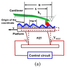
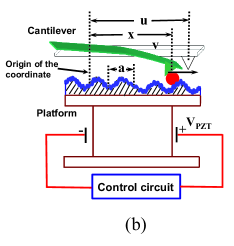
Figure 1: (color online) Schematic diagrams of the controlled nano manipulation system: (a) the control system in experiments in which the cantilever of the AFM is fixed and the platform moves; (b) the equivalent control system in which the platform is fixed while the cantilever moves. The two control systems (a) and (b) are equivalent if we fix the origin of the coordinate with the moving platform. “PZT” denotes the piezoelectric transducer. The deformation of the PZT is controlled by the voltage $V_{\rm PZT}$ added on the PZT. Thus, the relative position $u$ can be controlled as what we want by a control circuit.

When the cantilever tip moves on the substrate, the nano friction may occur on the contact area. In recent experiments Gnecco , the average frictional force is observed to be logarithmically dependent on the velocity of the cantilever tip $v=dx/dt$, i.e.,

$$\bar{F}_{f}=F_{f_{0}}+F_{f_{1}}\ln\left(\frac{v}{v_{1}}\right),$$ (2)

where $F_{f_{0}}$, $F_{f_{1}}$, $v_{1}$ are constant parameters. There also exists periodic lateral force induced by the surface potential of the substrate, and stochastic noises induced by the thermal motions of the substrate atoms. For simplicity, we only consider the fundamental-frequency component of the periodic lateral force, and omit the correlation effects of the thermal motions of the substrate atoms. Additionally, to simplify our discussions, the origin of coordinate is chosen such that the periodic lateral force is zero at the origin. Thus, the resulting modification of the lateral force can be expressed as:

$$\delta F_{f}=F_{f_{2}}\sin\left(2\pi\frac{x}{a}\right)-\xi(t),$$ (3)

where $F_{f_{2}}$ is the amplitude of the periodic lateral force; $a$ is the lattice constant of the substrate; and $\xi(t)$ is a white noise such that $E(\xi(t))=0$, $E(\xi(t)\xi(t^{\prime}))=D_{\xi}\delta(t-t^{\prime})$, with $D_{\xi}$ being the strength. $E\left(\cdot\right)$ denotes the ensemble average over the white noise.

From Eqs. (1), (2), and (3), the equations of the system can be expressed in the Ito notation as:

$$dx = vdt,$$

$$mdv = k_{c}(u-x)dt+\left[-F_{f_{0}}-F_{f_{1}}\ln\left(\frac{v}{v_{1}}\right)\right.$$ (4)

$$\left.-F_{f_{2}}\sin\left(2\pi\frac{x}{a}\right)\right]dt+\sqrt{D_{\xi}}dW,$$

where $m$ is the effective mass of the cantilever tip; and $dW=W\left(t+dt\right)-W\left(t\right)$ is the increment of the Wiener process $W\left(t\right)=\int_{0}^{t}\xi\left(\tau\right)d\tau$ satisfying:

$$E(dW)=0,\quad(dW)^{2}=dt.$$ (5)

III Stick-slip motion under open-loop control

In order to implement nano manipulation by the cantilever tip of the AFM with a constant velocity $v^{*}$, i.e., to control the position of the cantilever tip such that $x=v^{*}t$, a simple strategy is to set $u=v^{*}t$. However, this would be ineffective due to the existence of the periodic lateral force and the stochastic fluctuations especially when the roughness of the substrate is relatively large compared with the stiffness of the cantilever of the AFM. In such case, existing studies Tshiprut ; Socoliuc1 have predicted stick-slip motions of the cantilever tip, which greatly reduce the precision of the nano manipulation. The lateral pushing force imposed by the cantilever tip oscillates under the stick-slip motion, which can be so large that the fragile sample and substrate are damaged, or the cantilever tip of the AFM slide over them.

The drawbacks of the open-loop constant control can be seen from the following numerical examples. The system parameters are chosen as Tshiprut :

$$F_{f_{0}}=10\,\,{\rm nN},\quad F_{f_{1}}=1\,\,{\rm nN},\quad a=0.25\,\,{\rm nm},$$

$$v_{1}=1\,\,{\rm nm/s},\quad F_{f_{2}}=\,\,{\rm either}\,\,0.25\,\,{\rm nN}\,\,{\rm or}\,\,15\,\,{\rm nN},$$

$$v^{*}=3\,\,{\rm nm/s},\quad\sqrt{D_{\xi}}=0.1\,\,{\rm nN\cdot s^{-1/2}},$$

$$k_{c}=1\,\,{\rm N/m},\quad m=5\times 10^{-11}\,\,{\rm kg},$$ (6)

under which the simulation results of the position $x$, velocity $v$, and the lateral force $F_{p}$ imposed by the cantilever tip are shown in Fig. 2.

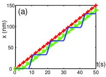
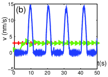
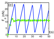
Figure 2: (color online) Plots of (a) the positions, (b) the velocities of the cantilever tip, and (c) the pushing forces imposed by the cantilever tip. The red curves with plus signs denote the ideal trajectories for which the cantilever tip moves with constant velocity $v=v^{*}=3$ nm/s; the green triangle (blue solid) curves represent the controlled trajectories under open-loop control $x=v^{*}t$, with the amplitudes of the periodic lateral force $F_{f_{2}}$ as $0.25$ nN ($15$ nN).

As shown in Fig. 2, when the amplitude of the periodic lateral force $F_{f_{2}}$ is relatively small such that $F_{f_{2}}/a$ is comparable with $k_{c}$ (the case with $F_{f_{2}}=0.25$ nN), which is the case when the cantilever tip moves on an incommensurate substrate PerssonBook , there exists no stick-slip motion and the cantilever tip moves with a constant velocity after a transient process (see the green triangle curves). However, when the amplitude of the periodic lateral force is relatively large such that $F_{f_{2}}/a\gg k_{c}$ (the case with $F_{f_{2}}=15$ nN), which may be valid when the cantilever tip moves on a commensurate substrate, stick-slip motions can be observed (see the blue solid curves). Such stick-slip motions can be explained by the elastic instability predicted by the Frenkel-Kontorova model PerssonBook . In this case, the cantilever tip moves only when the pushing force $F_{p}$ exceeds the critical value, i.e., the peak value of the sawtoothlike trajectory shown in Fig. 2(c). It is also shown in Fig. 2(a) that no matter whether the stick-slip motion occurs or not, there exist tracking errors between the controlled trajectories (the green triangle curve and the blue solid curve) and the ideal trajectory (the red curve with plus signs), which need to be compensated to improve the precision of the nano manipulation.

IV Reduction of the stick-slip motion by real-time feedback control

In this section, we introduce feedback control to reduce this unexpected stick-slip motion under open-loop control. The object of our method is to monitor the deformation of the cantilever and thus make the cantilever tip move with a given constant velocity.

To acquire feedback signals, there are two available sensing methods supported by the AFM-based nano manipulation systems: position sensing and force sensing. Position sensing is one of the basic functions of the AFM, by which one can easily obtain the tomography of a surface with nano-scale roughness. However, real-time position sensing is unavailable during the nano manipulation. Another sensing capacity of the AFM is the force sensing, which can be done by detecting the deformation of the cantilever of the AFM. In contrast with position sensing, force sensing can be done during the nano manipulation, which makes the real-time feedback control possible. The main idea of our feedback control method is to estimate the position of the cantilever tip by force sensing to adjust the control parameter $u$, and further control the motion of the tip. The control process thus can be divided into two steps, i.e., a filtering and estimation step and a feedback control step, which will be specified below.

IV.1 Position estimation by force sensing

By the force sensing capacity of the AFM, the pushing force measured can be expressed as:

$$F_{p}^{m}=k_{c}\left(u-x\right)+\eta(t),$$ (7)

where $\eta\left(t\right)$ is a white noise induced by the measurement apparatus. $\eta\left(t\right)$ satisfies

$$E\left(\eta\left(t\right)\right)=0,\quad E\left(\eta\left(t\right)\eta\left(t^{\prime}\right)\right)=D_{\eta}\delta\left(t-t^{\prime}\right),$$ (8)

where $D_{\eta}$ is the strength of the noise $\eta\left(t\right)$.

To reduce the measurement-induced disturbance of $\eta\left(t\right)$ in feedback control, we filter the measured signal $F_{p}^{m}$ by a low-pass filter over a time window $[t-T,t]$. The output signal can be expressed as (see, e.g., Refs. SarovarM ; Liuzhuo ):

$$\hat{F}_{p}^{m}\left(t\right)=\frac{1}{T}\int_{t-T}^{t}e^{-\gamma_{ft}\left(t-\tau\right)}F_{p}^{m}\left(\tau\right)d\tau,$$ (9)

where $\gamma_{ft}$ is the damping rate of the low-pass filter. Then, the position of the tip $x$ can be estimated from $\hat{F}_{p}^{m}$ by:

$$\hat{x}\left(t\right)=u(t)-\frac{1}{k_{c}}\hat{F}_{p}^{m}\left(t\right).$$ (10)

Under the filtering condition

$$\gamma_{ft}\ll 1/T,$$ (11)

it can be verified that

$$x\left(t\right)-\hat{x}\left(t\right)=e^{-\gamma_{ft}t}\left(x_{0}-\hat{x}_{0}\right),$$ (12)

where $x_{0}$ and $\hat{x}_{0}$ are the initial states of $x\left(t\right)$ and $\hat{x}\left(t\right)$ respectively (see the derivation in Appendix A). Thus, the estimated position $\hat{x}\left(t\right)$ exponentially converges to the position of the tip $x\left(t\right)$ with the convergence rate $\gamma_{ft}$, and thus $\hat{x}\left(t\right)$ can be taken as a good estimation of $x\left(t\right)$ when $t\gg 1/\gamma_{ft}$.

IV.2 Feedback control design based on the estimated position

Based on the estimated position $\hat{x}$ given in Eq. (10), we can design the position-based feedback control $u\left(\hat{x}\right)$ to reduce the stick-slip motion of the cantilever tip, which is given as follows:

$$u\left(\hat{x}\right) = \frac{1}{k_{c}}\left[k_{c}x^{*}+F_{f_{0}}+F_{f_{1}}\ln\left(\frac{v^{*}}{v_{1}}\right)+F_{f_{2}}\sin\left(2\pi\frac{\hat{x}}{a}\right)\right.$$ (13)

$$\left.-k_{x}\left(\hat{x}-x^{*}\right)-k_{I}\int_{0}^{t}\left(\hat{x}\left(\tau\right)-x^{*}\right)d\tau\right],$$

where $x^{*}=v^{*}t$ is the desired motion of the tip; and $k_{x},\,k_{I}>0$ are the control parameters to be determined. The term

$$k_{c}x^{*}+F_{f_{0}}+F_{f_{1}}{\rm ln}\left(v^{*}/v_{1}\right)+F_{f_{2}}\sin\left(2\pi\hat{x}/a\right)$$

in the control given by Eq. (13) is introduced to compensate the mean and the periodic friction forces. The proportional and integral feedback control terms $k_{x}\left(\hat{x}-x^{*}\right)$ and $k_{I}\int_{0}^{t}\left(\hat{x}-x^{*}\right)d\tau$ are introduced to speed up the convergence of the system dynamics to the stationary motion and reduce the static error.

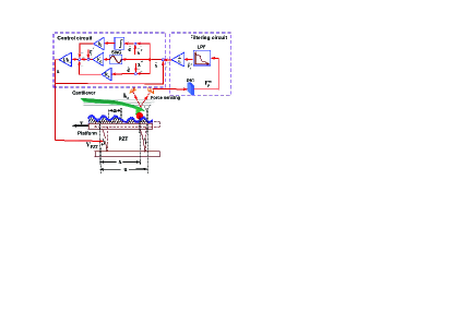
Figure 3: (color online) Schematic diagram of the feedback control loop, where $r^{*}=k_{c}x^{*}+F_{f_{0}}+F_{f_{1}}{\rm ln}\left(v^{*}/v_{1}\right)$ and $\hat{e}=\hat{x}-x^{*}$; “PZT”, “PEC”, “LPF”, and “SWG” are the piezoelectric transducer, the photonelectric convertor, the low-pass filter, and the sine-wave generator respectively. The feedback control circuit is divided into two parts, i.e., a filtering circuit and a control circuit The designed feedback control $u$ in Eq. (13) can be used to find the voltage $V_{\rm PZT}=V_{\rm PZT}\left(u\right)$ added on the PZT.

The schematic diagram of the feedback control proposed is given in Fig. 3. The deformation of the cantilever tip of the AFM is detected by an optical refracting system, and then converted into electric signals by a photonelectric convertor. The output signal masked by the measurement noise $\eta\left(t\right)$ is fed into a low-pass filter followed by a control circuit to generate the feedback control signal. The feedback electric signal is used to control the motion of the platform by adjusting the voltage $V_{\rm PZT}$ added on the piezoelectric transducer connected to the platform.

Under the filtering condition (11), the weak noise condition

$$D_{\xi}\ll 2F_{f_{1}}\left(k_{c}+k_{x}\right)a^{2}/v^{*},\,2F_{f_{1}}mv^{*},$$ (14)

and choosing the control parameters $k_{I}$ and $k_{x}$ such that

$$k_{I}<F_{f_{1}}\left(k_{c}+k_{x}\right)/mv^{*},$$ (15)

the controlled trajectory $x\left(t\right)$ tracks the desired trajectory $x^{*}=v^{*}t$ in average (see Appendix B), i.e.,

$$\lim_{t\rightarrow\infty}\left(E\left(x\left(t\right)\right)-x^{*}\right)=0,$$ (16)

where $E\left(\cdot\right)$ denotes the ensemble average of the stochastic signal. This result indicates that the stick-slip motion of the cantilever tip can be efficiently suppressed by the designed feedback control.

To evaluate the magnitude of the stochastic fluctuation, we further estimate the variances of the position $x$ and velocity $v$ of the cantilever tip, which are defined by:

$$V_{x}=E\left(\left(x-E\left(x\right)\right)^{2}\right),\quad V_{v}=E\left(\left(v-E(v)\right)^{2}\right).$$

With additional calculations, the stationary values of the variances $V_{x}$ and $V_{v}$ can be approximately estimated as (see the analysis in Appendix B):

$$V_{x}^{\infty}=\frac{D_{\xi}v^{*}}{2F_{f_{1}}\left(k_{c}+k_{x}\right)},\quad V_{v}^{\infty}=\frac{D_{\xi}v^{*}}{2F_{f_{1}}m}.$$ (17)

The effectiveness of our proposal can be demonstrated via numerical examples. Given the system parameters

$$F_{f_{0}}=10\,\,{\rm nN},\quad F_{f_{1}}=1\,\,{\rm nN},\quad a=0.25\,\,{\rm nm},$$

$$v_{1}=1\,\,{\rm nm/s},\quad F_{f_{2}}=15\,\,{\rm nN},$$

$$v^{*}=3\,\,{\rm nm/s},\quad\sqrt{D_{\xi}}=0.1\,\,{\rm nN\cdot s^{1/2}},$$

$$k_{c}=1\,\,{\rm N/m},\quad m=5\times 10^{-11}\,\,{\rm kg},\quad k_{I}=1\,\,{\rm N/\left(m\cdot s\right)},$$

$$k_{x}=5\,\,{\rm N/m},\quad T=0.1\,\,{\rm s},\quad\gamma_{ft}=1\,\,{\rm s}^{-1},$$ (18)

we compare the motions of the cantilever tip driven by the feedback control given in Eq. (13) and by the open-loop control $u=v^{*}t$. Each curve is obtained by averaging over $20$ sample (stochastic) trajectories. As shown in Fig. 4, the stick-slip motion observed under open-loop control (the green triangle curves) is greatly reduced by the proposed feedback control (the blue solid curves). To compare the stochastic fluctuations with the mean trajectories, we calculate the square roots of the variances $\sigma_{x}=V_{x}^{1/2}$ and $\sigma_{v}=V_{v}^{1/2}$. It can be obtained over $20$ stochastic trajectories that $\sigma_{x}^{\infty}=0.06$ nm and $\sigma_{v}^{\infty}=0.26$ nm/s, which are quite close to the estimated values $\sigma_{x}^{\infty}=0.05$ nm, $\sigma_{v}^{\infty}=0.38$ nm/s given by Eq. (17) and are negligible compared with the average motion ($E\left(x\right)$ is about tens of nm, and $E\left(v\right)$ is about $3$ nm/s).

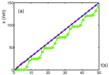
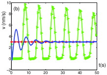
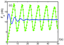
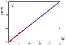
Figure 4: (color online) Plots of the motions of the cantilever tip with (a) the position $x$, (b) the velocity $v$, and (c) the lateral force $F_{p}$ imposed by the cantilever tip; (d) shows the trajectories in presence of parameter uncertainties given in Eq. (V). The red curves with plus signs are the ideal trajectories with $v=v^{*}=3$ nm/s; the green curves with triangle signs represent the trajectories driven by the open-loop control $u=v^{*}t$; and the blue solid curves denote the mean trajectories under the feedback control given in Eq. (13). The mean trajectories in the plot are obtained over $20$ stochastic trajectories.

V Robustness against parameter uncertainties

The system parameters involved in Eq. (IV.2) can be identified offline by, e.g., pre-designed nanofriction experiments. In practical experiments, we also need to consider the uncertainties in the system parameters which may deteriorate the performances of the nano manipulation. For example, the plastic deformation of the tip and the adhesion force between the tip and the substrate can lead to small deviation $\Delta k_{c}$ of the stiffness $k_{c}$ (typically $\Delta k_{c}/k_{c}<10\%$ in the literature Muller ). To reduce the effects of uncertainties, we add an integral control term $-k_{I}\int_{0}^{t}\left(\hat{x}-x^{*}\right)d\tau$ in Eq. (13) to reduce the static error induced by the uncertainties.

Denote the additive uncertainties in the system parameters $k_{c}$, $F_{f_{0}}$, $F_{f_{1}}$, $F_{f_{2}}$, $v_{1}$, and $a$ by $\Delta k_{c}$, $\Delta F_{f_{0}}$, $\Delta F_{f_{1}}$, $\Delta F_{f_{2}}$, $\Delta v_{1}$, $\Delta a$, and assume that there exists a phase offset $\Delta\phi$ in the sine function in Eq. (3). With the analysis given in Appendix C, the static tracking error can be controlled to zero, i.e., $\lim_{t\rightarrow\infty}\left(E\left(x\right)-x^{*}\right)=0$, if the uncertainties of the system parameters are not too large to satisfy

$$\Delta_{x}=\left|\Delta k_{c}\right|+2\pi\frac{F_{f_{2}}}{a^{2}}\left|\Delta a\right|+\frac{2\pi}{a}\left|\Delta F_{f_{2}}\right|<k_{c}+k_{x},$$

$$\left|\Delta F_{f_{1}}\right|<F_{f_{1}},$$ (19)

and the gain of the integrator $k_{I}$ is chosen such that

$$k_{I}<\left(F_{f_{1}}-\left|\Delta F_{f_{1}}\right|\right)\left(k_{c}+k_{x}-\Delta_{x}\right)/mv^{*}.$$ (20)

It can be seen that the proportional and integral feedback terms $k_{x}\left(\hat{x}-x^{*}\right)$, $k_{I}\int_{0}^{t}\left(\hat{x}-x^{*}\right)d\tau$ in the control (13) both contribute to the robustness of our method: (i) the integral term is used to reduce the static error; and (ii) the proportional term is used to increase the robustness of our method about the parameter uncertainty (the parameter regime given in Eqs. (V) and (20) is enlarged when we increase the control parameter $k_{x}$). Given the parameter uncertainties:

$$\Delta F_{f_{0}}=1\,\,{\rm nN},\,\,\,\Delta F_{f_{1}}=0.1\,\,{\rm nN},\,\,\,\Delta a=0.01\,\,{\rm nm},$$

$$\Delta F_{f_{2}}=0.1\,\,{\rm nN},\,\,\,\Delta k_{c}=0.1\,\,{\rm N/m},$$ (21)

Figure 4(d) shows that our method is still valid under the given parameter uncertainties (the controlled trajectory, i.e., the blue solid curve, matches very well with the ideal trajectory, i.e., the red curve with plus signs).

VI Conclusion

In summary, we propose a feedback control strategy to reduce the stick-slip motion of the cantilever tip in a AFM-based nano manipulation system. The feedback control is designed based on the position estimation of the cantilever tip obtained by the force sensing capacity of the AFM. Compared with open-loop control, our proposal can greatly reduce the stick-slip motion of the cantilever tip. Our method is robust against small uncertainties in the system parameters, e.g., the stiffness of the cantilever of the AFM, the lattice constant of the substrate, and the phase offset in the surface potential of the substrate.

Future study will be focused on extending the method to more practical cases. For example, as shown in our discussions, our designed feedback control is valid only under small uncertainties. More robust design should be developed for large uncertainties. Since the uncertainties in the model of the system can be reduced to a DC plus periodic disturbance, internal model principle is a good choice of the control design. Additionally, our control design can be naturally extended to the two-dimensional nano manipulation systems. More interesting results, such as the suppression of the S-shaped motion of the cantilever tip, are hopeful to be observed for the two-dimensional case.

Appendix A Derivation of Eq. (12)

From Eqs. (7) and (10), we have

$$u-x = \left(F_{p}^{m}-\eta\left(t\right)\right)/k_{c},$$ (22)

$$u-\hat{x} = \hat{F}_{p}^{m}/k_{c}.$$ (23)

It can be calculated from Eqs. (9) and (22) that

$$\frac{1}{T}\int_{t-T}^{t}e^{-\gamma_{ft}\left(t-\tau\right)}\left(u\left(\tau\right)-x\left(\tau\right)\right)d\tau$$ (24)

$$= \frac{1}{k_{c}}\left(\hat{F}_{p}^{m}-\frac{1}{T}\int_{t-T}^{t}e^{-\gamma_{ft}\left(t-\tau\right)}\eta\left(\tau\right)d\tau\right)$$

$$= \frac{1}{k_{c}}\left(\hat{F}_{p}^{m}-\frac{1}{T}\int_{0}^{T}e^{-\gamma_{ft}\tilde{\tau}}\eta\left(t-\tilde{\tau}\right)d\tilde{\tau}\right)$$

$$\approx \frac{1}{k_{c}}\left(\hat{F}_{p}^{m}-\frac{1}{T}\int_{0}^{T}\eta\left(t-\tilde{\tau}\right)d\tilde{\tau}\right)$$

$$= \frac{1}{k_{c}}\left(\hat{F}_{p}^{m}-\frac{1}{T}\int_{t-T}^{t}\eta\left(\tau\right)d\tau\right)$$

$$\approx \frac{1}{k_{c}}\hat{F}_{p}^{m}=u-\hat{x}.$$

Here, we have used the condition given in Eq. (11), i.e., $T\ll 1/\gamma_{ft}$, to obtain $e^{-\gamma_{ft}t}\approx 1$ when $t\in\left[0,T\right]$ and the ergodic property Peterse of the white noise $\eta\left(t\right)$ to replace the time average of $\eta\left(t\right)$ by its ensemble average, i.e.,

$$\frac{1}{T}\int_{t-T}^{t}\eta\left(\eta\right)d\tau\approx E\left(\eta\left(t\right)\right)=0.$$

Let us set

$$h\left(t\right) = u\left(t\right)-x\left(t\right),$$

$$\hat{h}\left(t\right) = u\left(t\right)-\hat{x}\left(t\right),$$

then from Eq. (24), i.e.,

$$\hat{h}\left(t\right)=\frac{1}{T}\int_{t-T}^{t}e^{-\gamma_{ft}\left(t-\tau\right)}h\left(\tau\right)d\tau,$$

we have

$$\frac{d}{dt}\hat{h}\left(t\right)=\frac{1}{T}\left(h\left(t\right)-e^{-\gamma_{ft}T}h\left(t-T\right)\right)-\gamma_{ft}h\left(t\right).$$ (25)

We assume that $g\left(T\right)=e^{\gamma_{ft}T}h\left(t+T\right)$, then we have

$$\frac{1}{T}\left(h\left(t\right)-e^{-\gamma_{ft}T}h\left(t-T\right)\right)=\frac{1}{T}\left(g\left(0\right)-g\left(-T\right)\right),$$

which can be replaced by

$$g^{\prime}\left(T\right)\left|{}_{T=0}\right.=\frac{d}{dt}h\left(t\right)+\gamma_{ft}h\left(t\right)$$

under the condition $T\ll 1/\gamma_{ft}$. Thus, Eq. (25) can be reexpressed as:

$$\frac{d}{dt}\left(\hat{h}-h\right)=-\gamma_{ft}\left(\hat{h}-h\right).$$ (26)

From the definition of $h$ and $\hat{h}$, we have

$$\frac{d}{dt}\left(\hat{x}-x\right)=-\gamma_{ft}\left(\hat{x}-x\right),$$ (27)

which means that $\hat{x}-x\rightarrow 0$ when $t\gg 1/\gamma_{ft}$, i.e., the estimated position of the cantilever tip $\hat{x}$ tracks the actual position $x$ in the long time limit.

Appendix B Derivation of Eqs. (16) and (17)

By substituting the feedback control law given in Eq. (13) into Eq. (II), we have

$$dx = vdt,$$

$$mdv = \left[-k_{c}\left(x-x^{*}\right)-k_{x}\left(\hat{x}-x^{*}\right)\right.$$

$$+F_{f_{2}}\sin\left(2\pi\frac{\hat{x}}{a}\right)-F_{f_{2}}\sin\left(2\pi\frac{x}{a}\right)$$

$$\left.-F_{f_{1}}\left({\rm ln}\frac{v}{v_{1}}-{\rm ln}\frac{v^{*}}{v_{1}}\right)-k_{I}q\right]dt+\sqrt{D_{\xi}}dW,$$

$$d\delta\hat{x} = -\gamma_{ft}\delta\hat{x}dt,\,\,\,dq=\left(\hat{x}-x^{*}\right)dt,$$ (28)

where $\delta\hat{x}=\hat{x}-x$ and $q=\int_{0}^{t}\left(\hat{x}-x^{*}\right)d\tau$.

By taking the ensemble average and denoting $\delta\bar{x}=E\left(x\right)-x^{*}$, $\delta\bar{v}=E\left(v\right)-v^{*}$, $\delta\bar{\hat{x}}=E\left(\delta\hat{x}\right)$, and $\bar{q}=E\left(q\right)$, we can expand the equation to the second-order quadratures to obtain:

$$\delta\dot{\bar{x}} = \delta\bar{v},$$

$$m\delta\dot{\bar{v}} = -\left(k_{c}+k_{x}\right)\delta\bar{x}+F_{f_{2}}\frac{2\pi}{a}\cos\left(2\pi\frac{x^{*}}{a}\right)\delta\bar{\hat{x}}$$

$$-k_{x}\delta\bar{\hat{x}}-\frac{F_{f_{1}}}{v^{*}}\delta\bar{v}+F_{f_{2}}\frac{8\pi^{3}}{a^{3}}V_{x}\cos\left(2\pi\frac{x^{*}}{a}\right)\delta\bar{\hat{x}}$$

$$+F_{f_{1}}\frac{V_{v}}{2v^{*2}}+O\left(\frac{\delta\bar{x}}{a}\frac{\delta\bar{\hat{x}}}{a}\right)+O\left(\frac{\delta\bar{v}^{2}}{v^{*2}}\right)$$

$$+O\left(\frac{V_{x}^{2}}{a^{4}}\frac{\delta\bar{\hat{x}}}{a}\right)+O\left(\frac{V_{v}^{2}}{v^{*4}}\right)-k_{I}\bar{q},$$

$$\delta\dot{\bar{\hat{x}}} = -\gamma_{ft}\delta\bar{\hat{x}},\,\,\,\dot{\bar{q}}=\delta\bar{x}+\delta\bar{\hat{x}},$$ (29)

where $V_{x}=E\left(x-E\left(x\right)\right)^{2}$ and $V_{v}=E\left(v-\left(v\right)\right)^{2}$ are the variances of $x$ and $v$; and $O\left(\cdot\right)$ denotes the higher-order terms. Since the nonlinear equation (B) is linearized near the origin $\left(0,0,0,0\right)^{T}$ in Eq. (B), we have introduced the Gaussian assumption to omit higher-order quadratures of $x$ and $v$. We can further omit the terms related to $V_{x}/a^{2}$ and $V_{v}/v^{*2}$ in Eq. (B). In fact, as shown in Eq. (17), we have $V_{x}^{\infty}\ll a^{2}$, $V_{v}^{\infty}\ll v^{*2}$ under the assumption (14). Thus, we have $V_{x}\ll a^{2}$ and $V_{v}\ll v^{*2}$ for sufficiently long time. Since we are just interested in the stationary behaviors of the system dynamics, we can omit the terms related to $V_{x}/a^{2}$ and $V_{v}/v^{*\,2}$.

With the above analysis, we can obtain the linearization equation of Eq. (B) in the neighborhood of $\left(\delta\bar{x},\delta\bar{v},\delta\bar{\hat{x}},\bar{q}\right)^{T}=\left(0,0,0,0\right)^{T}$. It can be easily verified that the characteristic equation of the coefficient matrix of the linearization equation is

$$\left(s+\gamma_{ft}\right)\left(s^{3}+\frac{F_{f_{1}}}{mv^{*}}s^{2}+\frac{\left(k_{c}+k_{x}\right)}{m}s+\frac{k_{I}}{m}\right)=0.$$

Since $k_{I}<F_{f_{1}}\left(k_{c}+k_{x}\right)/mv^{*}$ from Eq. (15), the real parts of the eigenvalues of the above equation are all negative. It means that the linearization equation is exponentially stable, and thus the original nonlinear equation (B) is asymptotically stable at the origin, which leads to the fact that $\lim_{t\rightarrow\infty}\left(E\left(x\right)-x^{*}\right)=0$.

To approximately estimate the stationary variances, we replace $\hat{x}$ by $x$, linearize Eq. (B), and omit higher-order correlation terms. It can be verified that $V_{x}$, $V_{v}$, and $C_{xv}$, i.e., the covariance between $x$ and $v$, satisfy the following equation

$$\left(\begin{array}[]{c}\dot{V}_{x}\\ \dot{V}_{v}\\ \dot{C}_{xv}\\ \end{array}\right) = \left(\begin{array}[]{ccc}0&0&2\\ 0&-\frac{2F_{f_{1}}}{mv^{*}}&-\frac{2\left(k_{c}+k_{x}\right)}{m}\\ -\frac{k_{c}+k_{x}}{m}&1&-\frac{F_{f_{1}}}{mv^{*}}\\ \end{array}\right)$$ (43)

$$\left(\begin{array}[]{c}V_{x}\\ V_{v}\\ C_{xv}\\ \end{array}\right)+\left(\begin{array}[]{c}0\\ \frac{D_{\xi}}{m^{2}}\\ 0\\ \end{array}\right).$$

To consider the stationary variances, the omission of the higher-order correlation terms to obtain Eq. (43) is reasonable, because $x-\hat{x}\rightarrow 0$ when $t\rightarrow\infty$, and higher-order correlation terms are small compared with $V_{x}$, $V_{v}$, and $C_{xv}$ under the weak noise assumption (14). From Eq. (43), we can calculate the stationary variances of $x$ and $v$ as:

$$V_{x}^{\infty}=\frac{D_{\xi}v^{*}}{2F_{f_{1}}\left(k_{c}+k_{x}\right)},\quad V_{v}^{\infty}=\frac{D_{\xi}v^{*}}{2F_{f_{1}}m}.$$

Appendix C Robustness analysis of our method

Let us replace the system parameters $k_{c}$, $F_{f_{0}}$, $F_{f_{1}}$, $F_{f_{2}}$, $v_{1}$, and $a$ in Eq. (B) by $k_{c}+\Delta k_{c}$, $F_{f_{0}}+\Delta F_{f_{0}}$, $F_{f_{1}}+\Delta F_{f_{1}}$, $F_{f_{2}}+\Delta F_{f_{2}}$, $v_{1}+\Delta v_{1}$, and $a+\Delta a$, and consider the phase offset $\Delta\phi$. We can expand the equation to the linear terms of the uncertainties $\Delta k_{c}$, $\Delta F_{f_{0}}$, $\Delta F_{f_{1}}$, $\Delta F_{f_{2}}$, $\Delta v_{1}$, $\Delta\phi$, and $\Delta a$. By neglecting the higher-order nonlinear terms, we can obtain

$$\delta\dot{\bar{x}} = \delta\bar{v},$$

$$m\delta\dot{\bar{v}} = -w_{x}\delta\bar{x}-w_{v}\delta\bar{v}-\left(k_{x}-F_{f_{2}}\frac{2\pi}{a}\cos\frac{x^{*}}{a}\right)\delta\bar{\hat{x}}$$

$$-k_{I}\bar{q}+w_{0},$$

$$\delta\dot{\bar{\hat{x}}} = -\gamma_{ft}\delta\bar{\hat{x}},\,\,\,\dot{\bar{q}}=\delta\bar{x}+\delta\bar{\hat{x}},$$ (44)

where

$$w_{x} = -\frac{2\pi}{a}\cos\left(2\pi\frac{x^{*}}{a}\right)\left(F_{f_{2}}\frac{\Delta a}{a}-\Delta F_{f_{2}}\right)$$

$$+\Delta k_{c}+k_{c}+k_{x},$$

$$w_{v} = \left(F_{f_{1}}+\Delta F_{f_{1}}\right)/v^{*},$$

$$w_{0} = \Delta F_{f_{0}}+{\rm ln}\left(\frac{v^{*}}{v_{1}}\right)\Delta F_{f_{1}}+\frac{F_{f_{1}}}{v_{1}}\Delta v_{1}$$

$$-\sin\left(2\pi\frac{x^{*}}{a}\right)\Delta F_{f_{2}}-F_{f_{2}}\cos\left(2\pi\frac{x^{*}}{a}\right)\Delta\phi.$$

The characteristic equation of the linear matrix of Eq. (C) can be expressed as:

$$\left(s+\gamma_{ft}\right)\left(s^{3}+w_{v}s^{2}+w_{x}s+k_{I}\right)=0.$$

It can be checked from Eqs. (V) and (20) that the real parts of the eigenvalues of the above equation are all negative. It means that there exists a stationary solution of the linearlization equation of Eq. (B), so does the original equation (B). Thus, we have $\dot{\bar{q}}=\delta\bar{x}+\delta\bar{\hat{x}}\rightarrow 0$ when $t\rightarrow\infty$. Furthermore, from $\delta\dot{\bar{\hat{x}}}=-\gamma_{ft}\delta\bar{\hat{x}}$, it can be verified that $\delta\bar{\hat{x}}\rightarrow 0$. Thus, we have $\lim_{t\rightarrow\infty}\delta\bar{x}=\lim_{t\rightarrow\infty}\left(E\left(x\right)-x^{*}\right)=0$.

References

- (1) R. P. Feynman, Engineering and Science magazine XXIII, 22 (1960).
- (2) G. Binnig, H. Rohrer, Ch. Gerber, and E. Weibel, Appl. Phys. Lett. 40, 178 (1982).
- (3) G. Binnig, C. F. Quate, and Ch. Gerber, Phys. Rev. Lett. 56, 930 (1986).
- (4) T. Junno, K. Deppert, L. Montelius, and L. Samuelson, Appl. Phys. Lett. 66, 3627 (1995).
- (5) M. Martin, L. Roschier, P. Hakonen, U. Parts, M. Paalanen, B. Schleicher, and E. I. Kauppinen, Appl. Phys. Lett. 73, 1505 (1998).
- (6) M. Guthold, M. R. Falvo, W. G. Matthews, S. Paulson, S. Washburn, D. A. Erie, R. Superfine, F. P. Brooks, and R. M. Taylor, IEEE/ASME Transactions on Mechatronics 5, 189 (2000).
- (7) M. Sitti and H. Hashimoto, IEEE/ASME Transactions on Mechatronics 5, 199 (2000).
- (8) M. Sitti and H. Hashimoto, IEEE/ASME Transactions on Mechatronics 8, 287 (2003).
- (9) G. Y. Li, N. Xi, M. M. Yu, and W. K. Fung, IEEE/ASME Transactions on Mechatronics 9, 358 (2004).
- (10) G. Y. Li, N. Xi, H. P. Chen, C. Pomeroy, and M. Prokos, IEEE/ASME Transactions on Mechatronics 4, 605 (2005).
- (11) X. J. Tian, N. Xi, Z. L. Dong, and Y. C. Wang, Ultramicroscopy 105, 336 (2005).
- (12) L. Q. Liu, Y. L. Luo, N. Xi, Y. C. Wang, J. B. Zhang, and G. Y. Li, IEEE/ASME Transactions on Mechatronics 13, 76 (2008).
- (13) Y. Zhang, L. Q. Liu, N. Xi, Y. C. Wang, Z. L. Dong, and U. C. Wejinya, J. Appl. Phys. 110, 114515 (2011).
- (14) B.N.J. Persson, Sliding Friction: Physical Prindiples and Applications (2nd ed.) (Springer-Verlag, Germany, 2000).
- (15) A. I. Volokitin and B.J.N. Persson, Rev. Mod. Phys. 79, 1291 (2007).
- (16) E. Gnecco, R. Bennewitz, T. Gyalog, Ch. Loppacher, M. Bammerlin, E. Meyer, and H.-J. Güntherodt, Phys. Rev. Lett. 84, 1172 (2000).
- (17) E. Riedo, E. Gnecco, R. Bennewitz, E. Meyer, and H. Brune, Phys. Rev. Lett. 91, 084502 (2003).
- (18) N. S. Tambe and B. Bhusham, Nanotecnology 16, 2309 (2005).
- (19) Z. Tshiprut, S. Zelner, and M. Urbakh, Phys. Rev. Lett. 102, 136102 (2009).
- (20) A. Socoliuc, R. Bennewitz, E. Gnecco, and E. Meyer, Phys. Rev. Lett. 92, 134301 (2004).
- (21) F. Heslot, T. Baumberger, B. Perrin, B. Caroli, and C. Caroli, Phys. Rev. E 49, 4973 (1994).
- (22) W. G. Conley, C. M. Krousgrill, and A. Raman, Tribology Letters 29, 23 (2008).
- (23) Y. Braiman, F. Family, and H.G.E. Hentschel, Phys. Rev. B 55, 5491 (1997).
- (24) Y. Braiman, J. Barhen, and V. Protopopescu, Phys. Rev. Lett. 90, 094301 (2003).
- (25) A. Socoliuc, E. Gnecco, S. Maier, O. Pfeiffer, A. Baratoff, R. Bennewitz, and E. Meyer, Science 313, 207 (2006).
- (26) R. Guerra, A. Vanossi, and M. Urbakh, Phys. Rev. E 78, 036110 (2008).
- (27) R. Capozza, A. Vanossi, A. Vezzani, and S. Zapperi, Phys. Rev. Lett. 103, 085502 (2009).
- (28) H. Iizuka, J. Nakamura, and A. Natori, Phys. Rev. B 80, 155449 (2009).
- (29) Y. Guo, Z. H. Qu, and Z. Y. Zhang, Phys. Rev. B 73, 094118 (2006).
- (30) Y. Guo and Z. H. Qu, Automatica 44, 2560 (2008).
-
(31)
M. Sitti, Teleoperated 2-D micro/nano manipulation using atomic force microscope (Ph.D. Thesis, 1999).
http://www.me.cmu.edu/faculty1/sitti/papers/main.pdf. - (32) F. Q. Huang, R. B. Wu, Z. Liu, L. Zhou, J. Zhang, and C. W. Li, Optimal design of feedforward controller for piezoelectric ceramic actuator based on Prandtl-Ishlinskii model, to be published.
- (33) M. Brokate, J. Sprekels, Hysteresis and Phase Transitions (Springer-verlag, Berlin, 1996).
- (34) M. Sarovar, H.-S. Goan, T. P. Spiller, and G. J. Milburn, Phys. Rev. A 72, 062327 (2005).
- (35) Z. Liu, L. L. Kuang, K. Hu, L. T. Xu, S. H. Wei, L. Z. Guo, X.-Q. Li, Phys. Rev. A 82, 032335 (2010).
- (36) M. K. Müller, R. H. Geiss, and D. C. Hurley, Ultramicroscopy 106, 466 (2006).
- (37) K. Petersen, Ergodic Theory (Cambridge Studies in Advanced Mathematics), (Cambridge University Press, Cambridge, 1990).