Symmetry-projected variational approach for ground and excited states of the two-dimensional Hubbard model

Abstract

We present a symmetry-projected configuration mixing scheme to describe ground and excited states, with well defined quantum numbers, of the two-dimensional Hubbard model with nearest-neighbor hopping and periodic boundary conditions. Results for the half-filled $2\times 4$, $4\times 4$, and $6\times 6$ lattices, as well as doped $4\times 4$ systems, compare well with available results, both exact and from other state-of-the-art approximations. We report spectral functions and density of states obtained from a well-controlled ansatz for the $(N_{e}\pm 1)$-electron system. Symmetry projected methods have been widely used for the many-body nuclear physics problem but have received little attention in the solid state community. Given their relatively low (mean-field) computational cost and the high quality of results here reported, we believe that they deserve further scrutiny.

I Introduction

Since the discovery of high-Tc superconductivity, HTCSC-1 there has been a growing interest in the properties of correlated two-dimensional (2D) electronic systems. Dagotto-review Within this context, the Hubbard model Hubbard-model_def1 has received a lot of attention since it is considered one of the simplest models still containing the relevant physics. Anderson-suggestion Renewed interest in the Hubbard Hamiltonian also comes from recent experiments optical-1 ; optical-2 with cold fermionic atoms in optical lattices which open the possibility for direct simulations of the model with lattice emulators. IBloch-revmodphys Hubbard-like models are also relevant to describe electronic properties within the active research field of graphene. CastroNeto-review

The repulsive Hubbard Hamiltonian is a very interesting model in theoretical physics. On the one hand, neither its hopping (one-body) nor its on-site interaction (two-body) terms favor any interesting magnetic ordering. On the other hand, when both of them combine into the full Hamiltonian a rich variety of interesting phenomena is displayed, for example, correlation-driven metal-insulator transitions, Gebhard-1 ferromagnetism, Nagaoka-theorem deviations from the standard Fermi-liquid results, Dagotto-Sch-nfl long-wavelength collective modes Chang-Shiwei and spatially inhomogeneous phases. ChiaChen-Shiwei The dimensionality of the model also challenges the theoretical tools at our disposal. Exact analytical solutions exist in the one-dimensional (1D) case text-Hubbard-1D whereas the present knowledge of the basic quantum mechanical properties of the 2D Hubbard Hamiltonian relies, to a large extent, on numerical techniques applied to the Hamiltonian itself or to its strong coupling approximations, i.e., the t-J, t-J^∗ and Heisenberg models. Dagotto-review ; Szczepanski ; Review-Heisenberg-model In particular, for the case of the full 2D Hubbard Hamiltonian, a very efficient Lanczos algorithm, Lanczos-Fano based on the classification of all the irreducible representations of the space group, has allowed systematic studies in the $4\times 4$ lattice.

Going beyond the present limits of exact diagonalization (ED) techniques requires a truncation strategy. A key issue is then how to truncate the model space while still being able to retain the most important degrees of freedom relevant for the description of a particular ground and/or excited state. Nowadays there are several methods at our disposal, some of them already heavily used to study 1D and 2D Hubbard models with variable degree of success. One that has been used with great success is the Quantum Monte Carlo Nightingale ; Raedt-MC ; Sorella-1 (QMC) approach. Another is the density matrix renormalization group DMRG-White ; Dukelsky-Pittel-RPP ; Scholl-RMP (DMRG) scheme that represents a very powerful and general decimation prescription. Currently, the DMRG algorithm is understood as an energy minimization within a class of low entanglement wavefunctions known as matrix product states Scholl-AP ; GChan (MPS) establishing an exciting link with quantum information perpectives. Cirac A very flexible entanglement encoding is also provided by the rapidly expanding research area of tensor network states TNPS-1 ; TNPS-2 ; TNPS-3 (TNS).

Variational principles also offer very powerful methods to study Hubbard-like models. For example, the dynamical variational principle, DVP-1 ; DVP-2 expressed in the language of Green’s functions and self-energies, Fetter-W provides us with the variational cluster approximation VCA-1 (VCA), the dynamical impurity approximation DIA-1 (DIA) and the dynamical mean field theory DMFT-1 (DMFT). Within this context, the self-energy-functional theory SFT-1 (SFT) has emerged as a conceptual framework in which the VCA, DIA and DMFT, as well as several extensions of them, can be specified by the choice of a reference system. In particular, the cluster extensions to DMFT have provided important insights into the physics of the 2D Hubbard model in aspects such as the Mott-Hubbard transition, the pseudogap in doped systems, and the phase diagram itself.maier2005 ; stanescu2006 DMFT and its cluster extensions are particularly valuable as they have been shown to be complementary to finite size simulations, maier2005 ; moukouri2001 ; huscroft2001 ; aryanpour2003 including ours. Here, we also refer the interested reader to recent work Zgid where a hierarchy of truncated configuration interaction (CI) expansions has been considered as a solver for quantum impurity models and DMFT.

In the present work, we explore an alternative avenue not only to describe ground state properties of the 2D Hubbard model but also to access excitation spectra which represent a basic fingerprint of quantum mechanical correlations in the considered lattices. A first step in this direction, based on symmetry-projected configuration mixing ideas originally employed in microscopic nuclear structure theory, Carlo-review was undertaken for the 1D Hubbard model Carlos-Hubbard-1D and is extended in the present work to the 2D Hubbard Hamiltonian with periodic boundary conditions (PBC).

For a given single-electron space, we construct the most general unitary Hartree-Fock (HF) transformation. rs ; Blaizot-Ripka Since this HF-transformation mixes all the spin and linear momentum quantum numbers of the single-electron basis states, the corresponding Slater determinant deliberately breaks the original spin and translational symmetries of the 2D Hubbard Hamiltonian. Therefore, as such, our symmetry-broken Slater determinant can be considered as a convenient mean-field starting point enlarging the space of trial wave functions. rs ; Blaizot-Ripka We restore the broken translational and spin symmetries with the help of linear and angular momentum projection operators. This symmetry restoration recovers the multi-determinantal character in our trial state keeping good spin and linear momentum quantum numbers. The Ritz variational principle rs ; Blaizot-Ripka is then applied to the projected energy, i.e., ours is a variation-after-projection (VAP) scheme. This procedure provides us with the optimal (variational) representation of a ground state, with well defined spin and linear momentum quantum numbers, via a single symmetry-projected configuration. Our VAP scheme is also very close in spirit to Projected Quasiparticle Theory PQT-reference-1 ; PQT-reference-2 (PQT) and is related to other variational approaches.Tomita-1 ; Tomita-2

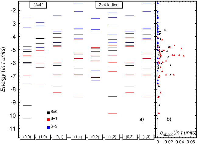
Figure 1: (Color online) The energy spectrum, obtained via Eq.(21), for the half-filled $2\times 4$ lattice at U=4t is shown in panel a). This spectrum can be hardly distinguished from the one obtained using an exact diagonalization (ED). Therefore, in panel b) the absolute errors are plotted for each of the predicted 120 solutions. For more details, see the main text.

In order to describe excited states with well defined quantum numbers, we construct a truncated basis consisting of a few (orthonormalized) symmetry-projected states throughout a chain of VAP calculations. This can be easily done, still with low computational cost, due to the simple structure of our projected wave functions. Finally, a further diagonalization of the 2D Hubbard Hamiltonian is performed within such a basis. With this configuration mixing procedure we may account, in a similar fashion, for additional correlations in both ground and excited states. In addition, our theoretical framework can be used to study important dynamical properties of the 2D Hubbard Hamiltonian like spectral functions. Dagotto-review ; Szczepanski ; Fetter-W

In this paper we have three main goals. First, we present the methodology of a VAP configuration mixing scheme, originally devised for the nuclear many-body problem, but not yet explored for the 2D Hubbard model. Therefore, in Sec. II we introduce our theoretical formalism. Symmetry restoration is described in Sec. II.1 while our configuration mixing scheme is outlined in Sec. II.2. For the reader’s convenience, the key ingredients of our approximations are stressed in these two sections while, to make our presentation self-contained, more technical details can be found in appendices A and B, respectively. Our second goal is to show how our theoretical framework can be used to access the spectral weight of states with different linear momentum quantum numbers. To this end, the computation of hole and particle spectral functions is briefly described in Sec. II.3 and more details are given in appendix C. Our third goal is to test the performance of our approximation for a selected set of illustrative examples. The results of our calculations for the half-filled $2\times 4$, $4\times 4$ and $6\times 6$ lattices are discussed in Sec. III. There, we pay attention to the properties of ground and excited states but also discuss hole and particle spectral functions as well as the corresponding density of states (DOS). In addition, in the case of the $4\times 4$ lattice, we consider doped systems with 14 and 15 electrons. Finally, Sec. IV is devoted to the concluding remarks and work perspectives.

II Theoretical Framework

In what follows, we describe the theoretical framework used in the present study. First, symmetry restoration and configuration mixing are presented in Secs. II.1 and II.2. The computation of spectral functions is briefly described in Sec. II.3.

II.1 Symmetry restoration for the 2D Hubbard model

We consider the following one-band version of the 2D Hubbard Hamiltonian Hubbard-model_def1

$$\hat{H}_{Hub} = -t\sum_{{\bf{j}}{\sigma}}\Big{(}\hat{c}_{{\bf{j}}+{\bf{x}}\sigma}^{\dagger}\hat{c}_{{\bf{j}}\sigma}+\hat{c}_{{\bf{j}}+{\bf{y}}\sigma}^{\dagger}\hat{c}_{{\bf{j}}\sigma}+h.c.\Big{)}$$ (1)

$$+ U\sum_{{\bf{j}}}\hat{c}_{{\bf{j}}\uparrow}^{\dagger}\hat{c}_{{\bf{j}}\downarrow}^{\dagger}\hat{c}_{{\bf{j}}\downarrow}\hat{c}_{{\bf{j}}\uparrow}$$

where the first term represents the nearest-neighbor hopping (t $>$ 0), with unit hopping vectors ${\bf{x}}=(1,0)$ and ${\bf{y}}=(0,1)$, and the second is the repulsive on-site interaction (U $>$ 0). The operators $\hat{c}_{{\bf{j}}\sigma}^{\dagger}$ and $\hat{c}_{{\bf{j}}\sigma}$ create and destroy a particle with spin-projection $\sigma=\pm 1/2$ (also denoted as $\sigma=\uparrow,\downarrow$) along an arbitrary chosen quantization axis on a lattice site ${\bf{j}}$=($j_{x},j_{y}$). They satisfy the usual anticommutation relations for fermion operators.Blaizot-Ripka Here, and in what follows, the lattice indices run as $j_{x}=1,\dots,N_{x}$ and $j_{y}=1,\dots,N_{y}$ with $N_{x}$ and $N_{y}$ being the number of sites along the x and y directions, respectively. The total number of sites is given by $N_{sites}=N_{x}\times N_{y}$. We assume PBC, i.e., the sites $N_{i}+1$ and 1, with i=x,y, are identical. Furthermore, we assume a lattice spacing $\Delta$=1.

Next, we apply the 2D Fourier transform

$$\hat{c}_{{\boldsymbol{\alpha}}\sigma}^{\dagger}=\frac{1}{\sqrt{N_{sites}}}\sum_{{\bf{j}}}e^{-i{\bf{k}}_{\alpha}{\bf{j}}}\hat{c}_{{\bf{j}}\sigma}^{\dagger}$$ (2)

to obtain operators with momentum ${\bf{k}}_{\alpha}=\left(k_{{\alpha}_{x}},k_{{\alpha}_{y}}\right)=\left(\frac{2\pi{\alpha}_{x}}{N_{x}},\frac{2\pi{\alpha}_{y}}{N_{y}}\right)$. The Hamiltonian (1) can be easily written in terms of these new operators. The quantum numbers ${\alpha}_{i}$, with i=x,y, take the allowed values

$${\alpha}_{i}=-\frac{N_{i}}{2}+1,\dots,\frac{N_{i}}{2}$$ (3)

inside the Brillouin zone (BZ). Ashcroft-Mermin-book Equivalently, they can take all integer values between 0 and $N_{i}-1$.

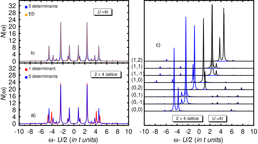
Figure 2: (Color online) The DOS ${\cal{N}}(\omega)$ [Eq.(30)] for the half-filled $2\times 4$ lattice at U=4t is plotted in panel a) as a function of the shifted excitation energy $\omega-U/2$ (in t units). Results have been obtained by approximating the ($N_{e}\pm 1$)-electron systems [Eqs. (23) and (27)] with $n_{T}=1$ (red) and $n_{T}=5$ (blue) Slater determinants out of Sec. II.1. As can be observed from panel b) the DOS obtained with exact diagonalization (ED) and the one obtained using $n_{T}=5$ HF-transformations can hardly be distinguished. The hole (blue) and particle (black) spectral functions, computed with $n_{T}=5$ HF-transformations, are plotted in panel c). A Lorentzian folding of width $\Gamma$=0.05t has been used.

In the HF-approximation, the ground state of an $N_{e}$-electron system is represented by a Slater determinant $|{\cal{D}}\rangle=\prod_{i=1}^{N_{e}}\hat{b}_{h}^{+}|0\rangle$ in which the energetically lowest $N_{e}$ single-electron states (hole states $h$, $h^{{}^{\prime}}$, …) are occupied while the remaining $2N_{sites}-N_{e}$ states (particle states $p$, $p^{{}^{\prime}}$, …) are empty. The HF-quasiparticle operators are given by

$$\hat{b}_{a}^{\dagger}=\sum_{{\boldsymbol{\alpha}}{\sigma}}{\cal{D}}_{{\boldsymbol{\alpha}}\sigma,a}^{*}\hat{c}_{{\boldsymbol{\alpha}}\sigma}^{\dagger}$$ (4)

where ${\cal{D}}$ is a general $2N_{sites}\times 2N_{sites}$ unitary transformation. rs ; Blaizot-Ripka In Eq. (4) $a$ is a shorthand notation for the set $(a_{x},a_{y},{\sigma}_{a})$. The transformation (4) mixes all the linear momentum quantum numbers as well as the spin projection of the states (2). As a consequence, $|{\cal{D}}\rangle$ deliberately breaks rotational (in spin space) and translational invariances. To restore the spin quantum numbers we explicitly use the projection operator

$$\hat{P}_{\Sigma{\Sigma}^{{}^{\prime}}}^{S}=\frac{2S+1}{8{\pi}^{2}}\int d\Omega{\cal{D}}_{\Sigma{\Sigma}^{{}^{\prime}}}^{S*}(\Omega)R_{S}(\Omega)$$ (5)

where $R_{S}(\Omega)=e^{-i\alpha\hat{S}_{z}}e^{-i\beta\hat{S}_{y}}e^{-i\gamma\hat{S}_{z}}$ is the rotation operator in spin space, $\Omega=\left(\alpha,\beta,\gamma\right)$ stands for the set of Euler angles and ${\cal{D}}_{\Sigma{\Sigma}^{{}^{\prime}}}^{S}(\Omega)$ are Wigner functions. Edmonds The form (5) has been frequently used for total angular momentum projection in nuclear physics. rs ; Carlo-review This form has also been adopted in the study of the 1D Hubbard model Carlos-Hubbard-1D and more recently within PQT in quantum chemistry. PQT-reference-1 ; PQT-reference-2

The linear momenta, $k_{{\xi}_{x}}$ and $k_{{\xi}_{y}}$, are restored with the projector

$$\hat{C}({\boldsymbol{\xi}})=\frac{1}{N_{sites}}\sum_{{\bf{j}}}e^{i\left(j_{x}+j_{y}\right)\hat{P}}e^{-i{\bf{k}}_{\xi}{\bf{j}}}$$ (6)

where $\hat{P}=\displaystyle\sum_{{\boldsymbol{\alpha}}\sigma}\left(k_{{\alpha}_{x}}+k_{{\alpha}_{y}}\right)\hat{c}_{{\boldsymbol{\alpha}}\sigma}^{\dagger}\hat{c}_{{\boldsymbol{\alpha}}\sigma}$ is the generator of the considered lattice translations. Note that this operator neither has vector character nor corresponds to the true linear momentum operator. It is associated with the quasi-momentum resulting from translational invariance of the lattice. We will refer to it, however, as linear momentum for simplicity. The projector (6) represents the 2D limit of the general operator restoring Galilei invariance. Carlo-review ; Rayner-Carlo-CM-1 ; Rayner-Carlo-CM-2 Note that, at variance with atomic nuclei, lattice systems can have solutions with linear momenta different from zero.

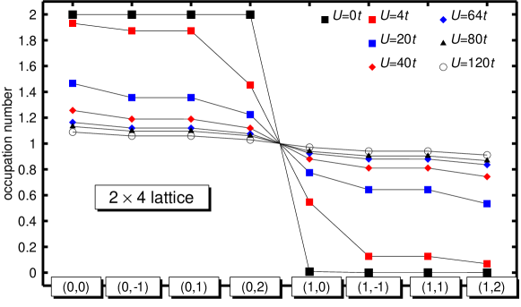
Figure 3: (Color online) Occupation numbers [Eq.(26)] of the basis states in the ground state of the half-filled $2\times 4$ lattice are plotted for various $U$ strengths.

In what follows, we introduce the shorthand notation $\Theta=(S,{\boldsymbol{\xi}})$ for the set of (symmetry) quantum numbers $(S,{\xi}_{x},{\xi}_{y})$, i.e., $\hat{P}_{\Sigma{\Sigma}^{{}^{\prime}}}^{S}\hat{C}({\boldsymbol{\xi}})=\hat{P}_{\Sigma{\Sigma}^{{}^{\prime}}}^{\Theta}$. We then use the following symmetry-projected wave function

$$|{\cal{D}};\Theta;\Sigma\rangle=\sum_{{\Sigma}^{{}^{\prime}}=-S}^{S}f_{{\Sigma}^{{}^{\prime}}}^{\Theta}\hat{P}_{\Sigma{\Sigma}^{{}^{\prime}}}^{\Theta}|{\cal{D}}\rangle$$ (7)

where $f_{{\Sigma}^{{}^{\prime}}}^{\Theta}$ are variational parameters. Note that, through the action of the projection operator $\hat{P}_{\Sigma{\Sigma}^{{}^{\prime}}}^{\Theta}$, the multi-determinantal character of the state characterized by the quantum numbers $\Theta$ and ${\Sigma}^{{}^{\prime}}$ is recovered and written in terms of the quantum numbers $\Theta$ and $\Sigma$. rs In practice, the integration over the set of Euler angles in Eq.(5) is discretized. For the integrals in $\alpha$ and $\gamma$ we have used 8 grid points whereas for the $\beta$-integration we have used 16 points. Therefore, the total number of grid points to be used for the projection operator $\hat{P}_{\Sigma{\Sigma}^{{}^{\prime}}}^{\Theta}$ is $1024\times N_{sites}$.

For a given symmetry $\Theta$, the energy (independent of $\Sigma$) associated with the state (7)

$$E^{\Theta}=\frac{f^{\Theta\dagger}{\cal{H}}^{\Theta}f^{\Theta}}{f^{\Theta\dagger}{\cal{N}}^{\Theta}f^{\Theta}}$$ (8)

is given in terms of the $(2S+1)\times(2S+1)$ Hamiltonian ${\cal{H}}_{{\Sigma}{\Sigma}^{{}^{\prime}}}^{\Theta}=\langle{\cal{D}}|\hat{H}_{Hub}\hat{P}_{\Sigma{\Sigma}^{{}^{\prime}}}^{\Theta}|{\cal{D}}\rangle$ and norm ${\cal{N}}_{{\Sigma}{\Sigma}^{{}^{\prime}}}^{\Theta}=\langle{\cal{D}}|\hat{P}_{\Sigma{\Sigma}^{{}^{\prime}}}^{\Theta}|{\cal{D}}\rangle$ matrices (see appendix A). It has to be minimized with respect to the coefficients $f^{\Theta}$ and the HF-transformation ${\cal{D}}$. The variation with respect to the mixing coefficients yields the following generalized eigenvalue equation

$$\left({\cal{H}}^{\Theta}-E^{\Theta}{\cal{N}}^{\Theta}\right)f^{\Theta}=0$$ (9)

with the constraint $f^{\Theta\dagger}{\cal{N}}^{\Theta}f^{\Theta}=1_{2S+1}$ ensuring the orthogonality of the solutions. The unrestricted minimization of the energy (8) with respect to the underlying HF-transformation ${\cal{D}}$ can be carried out via the Thouless theorem. rs ; Carlo-review The corresponding variational equations assume the form

$$M_{{\Theta}}^{-1\dagger}G^{\Theta}L_{\Theta}=0$$ (10)

with

$$G_{ph}^{\Theta}=\Big{[}f^{\Theta\dagger}\left({\cal{K}}^{\Theta}-E^{\Theta}{\cal{R}}^{\Theta}\right)f^{\Theta}\Big{]}_{ph}$$ (11)

Here, the $N_{e}\times N_{e}$ and $(2N_{sites}-N_{e})\times(2N_{sites}-N_{e})$ matrices $L_{{\Theta}}$ and $M_{{\Theta}}$ are obtained via the Cholesky decompositions. Carlo-review ; Rayner-Carlo-CM-1 The particle-hole kernels ${\cal{K}}_{\Sigma{\Sigma}^{{}^{\prime}}}^{\Theta;ph}=\langle{\cal{D}}|\hat{H}_{Hub}\hat{P}_{\Sigma{\Sigma}^{{}^{\prime}}}^{\Theta}{\hat{b}}^{\dagger}_{p}{\hat{b}}_{h}|{\cal{D}}\rangle$ and ${\cal{R}}_{\Sigma{\Sigma}^{{}^{\prime}}}^{\Theta;ph}=\langle{\cal{D}}|\hat{P}_{\Sigma{\Sigma}^{{}^{\prime}}}^{\Theta}{\hat{b}}^{\dagger}_{p}{\hat{b}}_{h}|{\cal{D}}\rangle$ are given in appendix B. It should be stressed that, for a given symmetry $\Theta$, we only retain the energetically lowest solution of Eqs.(9) and (10). Both the HF-transformation ${\cal{D}}$ and the mixing coefficients $f^{\Theta}$ are essentially complex, therefore one needs to minimize $n_{var}=2(2N_{sites}-N_{e})\times N_{e}+4S$ real variables. We use a quasi-Newton method for such a minimization. quasi-Newton-1 ; quasi-Newton-2 The variational procedure already described is known in nuclear structure physics as the VAMPIR (i.e., Variation After Mean field Projection In Realistic model spaces). Carlo-review Note, that particle number projection rs is not carried out in the present study since the considered Slater determinants conserve the number of electrons.

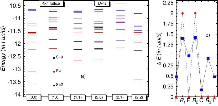
Figure 4: (Color online) The energy spectrum, obtained via Eq.(21), for the half-filled $4\times 4$ lattice at U=4t is shown in panel a). In panel b), the excitation energies from the ground state to the lowest-lying S=1 and S=2 states from panel a) are plotted as functions of the linear momentum quantum numbers $\Gamma=(0,0)$, $R_{1}=(1,0)$, $P=(2,0)$, $R_{2}=(2,1)$, $Q=(2,2)$, and $R_{3}=(1,1)$, respectively. In addition to U=4t (blue boxes), results for U=0t (red diamonds) are also included for comparison.

II.2 Symmetry-projected configuration mixing for the 2D Hubbard model

An accurate description of excited states in a many-fermion system is much more difficult even when one is usually interested in just a small fraction of the low-lying spectrum. Here, the main difficulty in the optimization of excited states is ensuring orthogonality among them and with respect to the ground state. For this, we simply use a Gram-Schmidt orthogonalization. Our goal in this section is to construct, throughout a chain of VAP calculations, a basis of a few (orthonormalized) states with well defined quantum numbers $\Theta$.

Suppose we have generated a ground state solution $|{\phi}^{1}\rangle=|{\cal{D}};\Theta;\Sigma\rangle$ out of Eqs. (9) and (10) in Sec. II.1. Then we write the first excited state wave function as

$$|{\varphi}_{2}\rangle={\beta}_{1}^{2}|{\phi}^{1}\rangle+{\beta}_{2}^{2}|{\phi}^{2}\rangle$$ (12)

where $|{\phi}^{2}\rangle$ has a form similar to Eq.(7) but with different coefficients $f^{2\Theta}$ and underlying HF-transformation ${\cal{D}}^{2}$. The label 2 distinguishes them from the ones (i.e., $f^{1\Theta}$ and ${\cal{D}}^{1}$) corresponding to the reference ground state we already have. Both ${\beta}_{1}^{2}$ and ${\beta}_{2}^{2}$ can be obtained by requiring that $\langle{\phi}^{1}|{\varphi}_{2}\rangle=0$ and $\langle{\varphi}_{2}|{\varphi}_{2}\rangle=1$. They are given in terms of the projector (i.e., $\hat{S}_{1}=\hat{S}_{1}^{2}$)

$$\hat{S}_{1}=\frac{|{\phi}^{1}\rangle\langle{\phi}^{1}|}{\langle{\phi}^{1}|{\phi}^{1}\rangle}$$ (13)

as follows

$${\beta}_{2}^{2} = \langle{\phi}^{2}|\left(1-\hat{S}_{1}\right)|{\phi}^{2}\rangle^{-1/2}$$

$${\beta}_{1}^{2} = -\frac{\langle{\phi}^{1}|{\phi}^{2}\rangle}{\langle{\phi}^{1}|{\phi}^{1}\rangle}{\beta}_{2}^{2}$$ (14)

The first excited state is obtained varying the energy functional for (12) with respect to $f^{2\Theta}$ and ${\cal{D}}^{2}$. For the second excited state, we introduce a new state $|{\phi}^{3}\rangle$, again with the same form as in Eq.(7), and write

$$|{\varphi}_{3}\rangle={\beta}_{1}^{3}|{\phi}^{1}\rangle+{\beta}_{2}^{3}|{\phi}^{2}\rangle+{\beta}_{3}^{3}|{\phi}^{3}\rangle$$ (15)

with coefficients ${\beta}_{1}^{3}$, ${\beta}_{2}^{3}$ and ${\beta}_{3}^{3}$ such that $|{\varphi}_{3}\rangle$ is orthogonal to the previous solutions $|{\varphi}_{1}\rangle=|{\phi}^{1}\rangle$ [Eq.(7)] and $|{\varphi}_{2}\rangle$ [Eq.(12)] as well as $\langle{\varphi}_{3}|{\varphi}_{3}\rangle=1$. The second excited state is obtained varying the energy functional for (15) with respect to $f^{3\Theta}$ and ${\cal{D}}^{3}$. Let us have a more general situation in which, by successive variation, $i=1,\dots,m-1$ orthonormalized solutions (for example, $|{\varphi}_{1}\rangle$ and $|{\varphi}_{2}\rangle$)

$$|{\varphi}_{i}\rangle=\sum_{j=1}^{i}|{\phi}^{j}\rangle{\beta}_{j}^{i}$$ (16)

are already at our disposal. Each of the states $|{\phi}^{j}\rangle$ in (16) has the same form as (7). One then writes the ansatz for the $m$th state wave function (for example, $|{\varphi}_{3}\rangle$) as

$$|{\varphi}_{m}\rangle=\sum_{j=1}^{m-1}|{\phi}^{j}\rangle{\beta}_{j}^{m}+|{\phi}^{m}\rangle{\beta}_{m}^{m}$$ (17)

with $|{\phi}^{m}\rangle$ having again the form (7). Requiring orthonormalization with respect to all the previous $m-1$ solutions (16) the coefficients ${\beta}_{m}^{m}$ and ${\beta}_{j}^{m}$ in Eq.(17) read

$${\beta}_{m}^{m} = \langle{\phi}^{m}|\left(1-\hat{S}_{m-1}\right)|{\phi}^{m}\rangle^{-1/2}$$

$${\beta}_{j}^{m} = -\sum_{k=1}^{m-1}\frac{\langle{\phi}^{k}|{\phi}^{m}\rangle}{\langle{\phi}^{j}|{\phi}^{k}\rangle}{\beta}_{m}^{m}$$ (18)

in terms of the projector (i.e., $\hat{S}_{m-1}=\hat{S}_{m-1}^{2}$)

$$\hat{S}_{m-1}=\sum_{j,k=1}^{m-1}\frac{|{\phi}^{j}\rangle\langle{\phi}^{k}|}{\langle{\phi}^{j}|{\phi}^{k}\rangle}$$ (19)

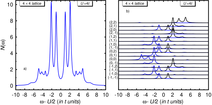
Figure 5: (Color online) The DOS ${\cal{N}}(\omega)$ [Eq.(30)] for the half-filled $4\times 4$ lattice at U=4t is plotted in panel a) as a function of the shifted excitation energy $\omega-U/2$ (in t units). Results have been obtained by approximating the ($N_{e}\pm 1$)-electron systems [Eqs. (23) and (27)] with $n_{T}=5$ HF-determinants. Hole (blue) and particle (black) spectral functions, are displayed in panel b). A Lorentzian folding of width $\Gamma$=0.2t has been used.

The energy for the state (17) takes the form

$$E^{m\Theta}=\frac{f^{m\Theta\dagger}{\cal{H}}^{m\Theta}f^{m\Theta}}{f^{m\Theta\dagger}{\cal{N}}^{m\Theta}f^{m\Theta}}$$ (20)

with kernels ${\cal{H}}_{\Sigma{\Sigma}^{{}^{\prime}}}^{m\Theta}$ and ${\cal{N}}_{\Sigma{\Sigma}^{{}^{\prime}}}^{m\Theta}$ accounting for the fact that $m$-1 linearly independent solutions have been removed from the variational space. Their expressions are slightly more involved Carlo-review than the ones required in Eq.(8) but still straightforward. They require the knowledge of the symmetry-projected matrix elements between two different Slater determinants $|{\cal{D}}^{i}\rangle$ and $|{\cal{D}}^{k}\rangle$ (see appendix A). The variation of the energy (20) with respect to $f^{m\Theta}$ yields an equation similar to (9) with the constraint $f^{m\Theta\dagger}{\cal{N}}^{m\Theta}f^{m\Theta}=1_{2S+1}$. The unrestricted minimization of the energy (20) with respect to ${\cal{D}}^{m}$, via the Thouless theorem, leads to variational equations similar to (10) but with kernels ${\cal{K}}_{\Sigma{\Sigma}^{{}^{\prime}}}^{m\Theta;ph}$ and ${\cal{R}}_{\Sigma{\Sigma}^{{}^{\prime}}}^{m\Theta;ph}$ that require symmetry-projected particle-hole matrix elements between two different Slater determinants $|{\cal{D}}^{i}\rangle$ and $|{\cal{D}}^{k}\rangle$ (see appendix B).

The procedure outlined in this section is known in nuclear structure physics as EXCITED VAMPIR. Carlo-review It provides a (truncated) basis of m (orthonormalized) states $|{\varphi}_{j}\rangle$, with a well defined symmetry $\Theta$, still keeping low computational cost. This is doable due to the simple structure of the projected states defining such a basis in combination with a fast minimization scheme. quasi-Newton-1 ; quasi-Newton-2 Our method can also be extended to use general Hartree-Fock-Bogoliubov (HFB) transformations. rs ; Carlo-review ; PQT-reference-1 However, this requires an additional projection of the particle number, which increases the numerical effort by about one order of magnitude and has hence not been used in the present paper.

It should be noticed that the ground state $|{\varphi}_{1}\rangle$ [Eq.(7)] is written as a projection operator acting on a single determinant, the first excited state $|{\varphi}_{2}\rangle$ [Eq.(12)] as a projection operator acting on two determinants, and so on. Because this allows excited state wave functions to be described at a higher level of quality than is the ground state wave function, our final step is to diagonalize the 2D Hubbard Hamiltonian in the basis of the states $|{\varphi}_{j}\rangle$.

$$\sum_{j=1}^{m}\Big{[}\langle{\varphi}_{i}|\hat{H}_{Hub}|{\varphi}_{j}\rangle-{\epsilon}_{\alpha}^{\Theta}{\delta}_{ij}\Big{]}C_{j\alpha}^{\Theta}=0$$ (21)

For ground and excited states, the resulting wave functions

$$|{\Omega}_{\alpha}^{\Theta}\rangle=\sum_{\alpha}C_{j\alpha}^{\Theta}|{\varphi}_{j}\rangle$$ (22)

may account for more correlations than the description based on a single symmetry-projected configuration discussed in Sec. II.1. In the present work, as a first step, we have restricted ourselves to test the performance of our approximation with $m$=5 (orthonormalized) states. As we will see, this turns out to be a reasonable starting point for, at least, a qualitative description of the considered lattices.

An interesting issue is the evolution of the energy of each state with the number $m$ of transformations included in the prescription described in this section. We observe that, for the lattices considered in the present study, the energy of the ground and the first couple of excited states remains unchanged when $m$ goes from 1 to 5 (the changes in the energy per site are of the order $10^{-4}$). This is partly because the main correlations have already been accounted for with a single symmetry-projected determinant. Therefore, the excited configurations obtained constitute reasonably good approximations to the true excited states of the considered system. We produce $m$=5 symmetry-projected determinants in order to obtain the low-lying spectrum. For the systems considered in this work, these states turn out to be weakly coupled through the Hamiltonian. However, this cannot be anticipated a priori and the diagonalization Eq.(21) should always be carried out. Preliminary results for larger square lattices (i.e., $8\times 8$ and $10\times 10$) as well as for other Hamiltonians (i.e., the $t-t^{{}^{\prime}}-U$ and $t-t^{{}^{\prime}}-t^{"}-U$ Hubbard models) indicate that there are cases in which the diagonalization Eq.(21) brings a sizeable amount of additional correlations.

II.3 Hole and particle spectral functions

Let us assume that for an even number $N_{e}$ of electrons we already have the ground state wave function $|{\cal{D}}^{1};{\Theta}^{0};\Sigma=0\rangle$, out of the calculations described in Sec. II.1. Since for all the considered lattices with an even number of electrons the ground state has spin S=0, but not neccessarily linear momenta zero, we write its quantum numbers as ${\Theta}^{0}=(0,{\boldsymbol{\xi}}^{0})$. Usually, spectral functions are computed within a Green’s function perspective. Fetter-W The key point is then to approximate the ground states of the $(N_{e}\pm 1)$-electron systems by a suitable ansatz. In the present study, we approximate Carlos-Hubbard-1D the ground state of the ($N_{e}$-1)-electron system, with the symmetry ${\Theta}^{-}=(S=1/2,{\boldsymbol{\xi}}^{-})$, by

$$|h_{1};{\Theta}^{-};\sigma\rangle = \sum_{ih{\sigma}^{{}^{\prime}}}f_{ih{\sigma}^{{}^{\prime}},h_{1}}^{{\Theta}^{-}}\hat{P}^{{\Theta}^{-}}_{\sigma{\sigma}^{{}^{\prime}}}\hat{b}_{h}({\cal{D}}^{i})|{\cal{D}}^{i}\rangle$$ (23)

where the index i runs as $i=1,\dots,n_{T}$, the hole index h as $h=1,\dots,N_{e}$ and ${\sigma}^{{}^{\prime}}=\pm 1/2$. In Eq.(23), we write $\hat{b}_{h}({\cal{D}}^{i})$ to explicitly indicate that holes are made on $n_{T}$ different Slater determinants. The determinants $|{\cal{D}}^{1}\rangle$ and $|{\cal{D}}^{i}\rangle$ correspond to the ground and lowest energy ($i=2,\dots,n_{T}$) states obtained for the $N_{e}$-electron system out of the calculations described in Sec. II.1. In the present study, we have restricted ourselves to a maximum of $n_{T}=5$ HF-transformations. The coefficients $f^{{\Theta}^{-}}$ in Eq.(23) are obtained by solving the equation

$$\left({\cal{H}}^{{\Theta}^{-}}-E_{h_{1}}^{{\Theta}^{-}}{\cal{N}}^{{\Theta}^{-}}\right)f^{{\Theta}^{-}}=0$$ (24)

that yields $2n_{T}N_{e}$ hole solutions $h_{1}$ with energies $E_{h_{1}}^{{\Theta}^{-}}$. With all the previous ingredients, one can compute Edmonds ; Rayner-Carlo-CM-1 ; Rayner-Carlo-CM-2 the hole spectral function as $S_{h_{1}}({\boldsymbol{\xi}}^{-},\delta\epsilon_{h_{1}})=|\langle h_{1};{\Theta}^{-}||{\hat{c}}_{{\boldsymbol{\xi}}^{0}-{\boldsymbol{\xi}}^{-}}||{\cal{D}}^{1};{\Theta}^{0}\rangle|^{2}$ in terms of the reduced matrix element

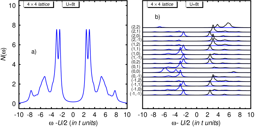
Figure 6: (Color online) The same as Fig.5 but for U=8t. The shapes of the DOS as well as the spectral functions for momenta $(\pi,0)$, $(\pi/2,0)$ and $(0,0)$ are qualitatively similar to the ones obtained using Lanczos calculations. Dagotto-RC-3184

$$\langle h_{1};{\Theta}^{-}||{\hat{c}}_{{\boldsymbol{\xi}}^{0}-{\boldsymbol{\xi}}^{-}}||{\cal{D}}^{1};{\Theta}^{0}\rangle=-\frac{1}{8{\pi}^{2}N_{sites}}\sqrt{\frac{2}{\langle{\cal{D}}^{1}|\hat{P}_{00}^{{\Theta}^{0}}|{\cal{D}}^{1}\rangle}}\times$$

$$\sum_{ihh^{{}^{\prime}}{\sigma}{\sigma}^{{}^{\prime}}}f_{ih{\sigma},h_{1}}^{{\Theta}^{-}*}\sum_{\boldsymbol{j}}e^{-i{\bf{k}}_{\xi}{\bf{j}}}\int d\Omega D_{\sigma{\sigma}^{{}^{\prime}}}^{1/2*}(\Omega)(-1)^{1/2-{\sigma}^{{}^{\prime}}}\times$$

$${\cal{D}}^{1*}_{{\boldsymbol{\xi}}^{0}-{\boldsymbol{\xi}}^{-}-{\sigma}^{{}^{\prime}},h^{{}^{\prime}}}\Big{[}{\cal{X}}_{h^{{}^{\prime}}h}^{i1}(\Omega,{\boldsymbol{j}})\Big{]}^{-1}n^{i1}(\Omega,{\boldsymbol{j}})$$ (25)

where ${\bf{k}}_{\xi}=\left(k_{{\xi}_{x}^{-}},k_{{\xi}_{y}^{-}}\right)=\left(\frac{2\pi{\xi}_{x}^{-}}{N_{x}},\frac{2\pi{\xi}_{y}^{-}}{N_{y}}\right)$. The indices i, $h,h^{{}^{\prime}}$ and $\sigma,{\sigma}^{{}^{\prime}}$ run as in (23), ${\xi}_{x}^{-}$ and ${\xi}_{y}^{-}$ run as in Eq.(3) and $\delta\epsilon_{h_{1}}=E^{{\Theta}^{0}}-E_{h_{1}}^{{\Theta}^{-}}$. Details for the computation of the kernels ${\cal{H}}^{{\Theta}^{-}}$ and ${\cal{N}}^{{\Theta}^{-}}$ in Eq.(24) as well as $\Big{[}{\cal{X}}_{h^{{}^{\prime}}h}^{i1}(\Omega,{\boldsymbol{j}})\Big{]}^{-1}$ and $n^{i1}(\Omega,{\boldsymbol{j}})$ in Eq.(II.3) can be found in appendices C and A, respectively. The occupation number $n({\boldsymbol{\xi}}^{-})$ of a basis state (2) in the $N_{e}$-electron ground state can be computed as

$$\sum_{h_{1}=1}^{2n_{T}N_{e}}S_{h_{1}}({\boldsymbol{\xi}}^{-},\delta\epsilon_{h_{1}})=n({\boldsymbol{\xi}}^{-})$$ (26)

The ($N_{e}$+1)-electron system, with the symmetry ${\Theta}^{+}=(S=1/2,{\boldsymbol{\xi}}^{+})$, is approximated by Carlos-Hubbard-1D

$$|p_{1};{\Theta}^{+};\sigma\rangle = \sum_{ip{\sigma}^{{}^{\prime}}}g_{ip{\sigma}^{{}^{\prime}},p_{1}}^{{\Theta}^{+}}\hat{P}^{{\Theta}^{+}}_{\sigma{\sigma}^{{}^{\prime}}}\hat{b}^{\dagger}_{p}({\cal{D}}^{i})|{\cal{D}}^{i}\rangle$$ (27)

where the index i runs again as in (23). The particle index p takes the values $p=N_{e}+1,\dots,2N_{sites}$ and ${\sigma}^{{}^{\prime}}=\pm 1/2$. In this case, the coefficients $g^{{\Theta}^{+}}$ are obtained by solving the equation

$$\left({\cal{H}}^{{\Theta}^{+}}-E_{p_{1}}^{{\Theta}^{+}}{\cal{N}}^{{\Theta}^{+}}\right)g^{{\Theta}^{+}}=0$$ (28)

that yields $2n_{T}(2N_{sites}-N_{e})$ particle solutions $p_{1}$ with energies $E_{p_{1}}^{{\Theta}^{+}}$. The particle spectral function is then written as $S_{p_{1}}({\boldsymbol{\xi}}^{+},\delta\epsilon_{p_{1}})=|\langle p_{1};{\Theta}^{+}||{\hat{c}}_{{\boldsymbol{\xi}}^{+}-{\boldsymbol{\xi}}^{0}}||{\cal{D}}^{1};{\Theta}^{0}\rangle|^{2}$ in terms of the reduced matrix element

$$\langle p_{1};{\Theta}^{+}||{\hat{c}}_{{\boldsymbol{\xi}}^{+}-{\boldsymbol{\xi}}^{0}}||{\cal{D}}^{1};{\Theta}^{0}\rangle=-\frac{1}{8{\pi}^{2}N_{sites}}\sqrt{\frac{2}{\langle{\cal{D}}^{1}|\hat{P}_{00}^{{\Theta}^{0}}|{\cal{D}}^{1}\rangle}}\times$$

$$\sum_{ipp^{{}^{\prime}}{\sigma}{\sigma}^{{}^{\prime}}}g_{ip\sigma,p_{1}}^{{\Theta}^{+}*}\sum_{\boldsymbol{j}}e^{-i{\bf{k}}_{\xi}{\bf{j}}}\int d\Omega D_{\sigma{\sigma}^{{}^{\prime}}}^{1/2*}(\Omega)n_{pp^{{}^{\prime}}}^{i1}(\Omega,{\boldsymbol{j}})\times$$

$${\cal{D}}^{1*}_{{\boldsymbol{\xi}}^{+}-{\boldsymbol{\xi}}^{0}{\sigma}^{{}^{\prime}},p^{{}^{\prime}}}n^{i1}(\Omega,{\boldsymbol{j}})$$ (29)

where, in this case, ${\bf{k}}_{\xi}=\left(k_{{\xi}_{x}^{+}},k_{{\xi}_{y}^{+}}\right)=\left(\frac{2\pi{\xi}_{x}^{+}}{N_{x}},\frac{2\pi{\xi}_{y}^{+}}{N_{y}}\right)$. The indices i, $p,p^{{}^{\prime}}$ and $\sigma$, ${\sigma}^{{}^{\prime}}$ run as in (27), ${\xi}_{x}^{+}$ and ${\xi}_{y}^{+}$ run as in Eq.(3) and $\delta\epsilon_{p_{1}}=E_{p_{1}}^{{\Theta}^{+}}-E^{{\Theta}^{0}}$. Details for the computation of the kernels ${\cal{H}}^{{\Theta}^{+}}$ and ${\cal{N}}^{{\Theta}^{+}}$ as well as $n_{pp^{{}^{\prime}}}^{i1}(\Omega,{\boldsymbol{j}})$ in Eq.(II.3) can be found in appendix C.

Finally, the DOS can be computed as

$${\cal{N}}(\omega)=\sum_{{\boldsymbol{\xi}}}\Big{[}S_{(h_{1})}({\boldsymbol{\xi}},\omega)+S_{(p_{1})}({\boldsymbol{\xi}},\omega)\Big{]}$$ (30)

where the indices $h_{1}$ and $p_{1}$ are absorbed into the continuous variable $\omega$. Due to the finite size of the system the spectral functions consist of a finite number of $\delta$ functions with different weights. Therefore, we introduce an artificial width $\Gamma$ for each state using a Lorentzian. In all cases our DOS is normalized to 2 $\times$ $N_{sites}$.

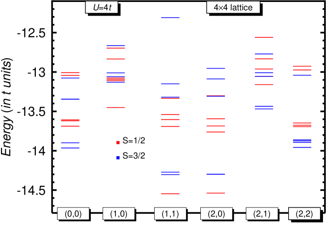
Figure 7: (Color online) Energy spectrum, obtained via Eq.(21), for the $4\times 4$ lattice with $N_{e}=15$ electrons at U=4t.

III Discussion of results

In this section, we discuss the results of our study. We have considered the $2\times 4$ half-filled lattice as a prototypical system where one can obtain the full spectrum by means of ED. This allows us to callibrate our approximation not only for ground state properties but also for excited states. Next, we have considered the well-studied half-filled $4\times 4$ lattice, which constitutes the largest square lattice for which exact ground state energies are available in the literature. Other approximation schemes have also been tested for this lattice in previous works. Results have already been published for doped systems with 14 and 15 electrons in this lattice, which motivated us to also perform calculations for them in the present study. Last, we consider the half-filled $6\times 6$ lattice as a prototype of a system where ED is no longer feasible. Many of the results to be discussed in what follows correspond to U=4t taken as a representative on-site repulsion for which studies are available. Nevertheless, let us stress that our formalism can be used for any 2D Hubbard hamiltonian of the form (1) with arbitrary U and/or t values.

III.1 The square $2\times 4$ lattice

Let us start by considering the rectangular $2\times 4$ lattice. The first five solutions obtained at half-filling via Eq.(21), for each of the linear momentum quantum numbers (0,0), (0,1), (0,2), (0,3), (1,0), (1,1), (1,2) and (1,3) and the spins S=0,1, and 2, are plotted in panel a) of Fig.1 for U=4t. The first excited state corresponds to a $\Theta=(1,1,2)$ configuration [with linear momenta $(\pi,\pi)$]. The energies ${\epsilon}_{\alpha}^{\Theta}$ of the 120 solutions shown in the figure, have been compared to the ones obtained using an ED. Albuquerque The comparison reveals that both spectra follow the same qualitative trend and can hardly be distinguished. Therefore in panel b) of the same figure, we have plotted the absolute errors $e_{absol.}=E_{exact}-E$ for each of the predicted 120 states. Our approximation fairly reproduces the exact ground state energy -10.2529t for this system. For all the 40 S=0 and S=1 solutions considered the absolute errors remain very small, the largest deviation being 0.047t for the second state with the symmetry $\Theta=(1,0,0)$. The previous results are encouraging if one takes into account that, even for this relatively small lattice, the number of variational parameters in our approximation $n_{var}$($S=0,{\xi}_{x},{\xi}_{y})=128$ and $n_{var}$($S=1,{\xi}_{x},{\xi}_{y})=132$ is about half of the dimensions $n_{RH}$($S=0,{\xi}_{x},{\xi}_{y})=221$ and $n_{RH}$($S=1,{\xi}_{x},{\xi}_{y})=294$ of the restricted Hilbert spaces. On the other hand, $n_{var}$($S=2,{\xi}_{x},{\xi}_{y})=136$ is larger than $n_{RH}$($S=2,{\xi}_{x},{\xi}_{y})=90$ and therefore our solutions reproduce the ED ones for S=2 states.

In panel a) of Fig. 2, we have plotted the DOS ${\cal{N}}(\omega)$ [Eq.(30)] for the half-filled $2\times 4$ lattice at U=4t. The calculations have been carried out by approximating the ($N_{e}$ $\pm$ 1)-electron systems [see Eqs. (23) and (27)] with $n_{T}$=1 (red curve) and $n_{T}$=5 (blue curve) HF-transformations along the lines described in Sec. II.3. We have introduced a shift equal to the chemical potential at half-filling (${\mu}_{0}=U/2$) so that the DOS in Fig.2 appears to be symmetric around $\omega$-U/2=0. This convention, i.e., to plot DOS and spectral functions vs. $\omega$-U/2 will be adopted in the rest of the paper. The DOS shows the Hubbard gap, $\Delta_{H}=U/2=2t$, characteristic of finite size lattices. We note, however, that previous studies within the framework of the dynamical cluster approximation (DCA) have shown that the gap is preserved at sufficiently low temperatures even in the thermodynamic limit (TDL). moukouri2001 ; huscroft2001 ; aryanpour2003 On the other hand, the nonperturbative study of Ref. 59 has concluded that for the half-filled Hubbard model the gap persists for any finite value of the on-site repulsion U, the only singular point being U=0t.

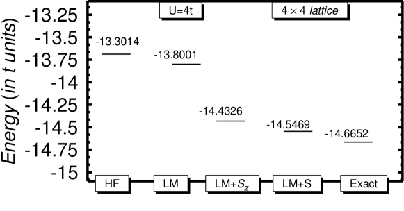
Figure 8: Ground state energy of the $4\times 4$ lattice with $N_{e}=15$ electrons at U=4t computed with various approaches. The different columns refer to the unprojected Hartree-Fock (HF) calculation, HF with linear momentum projection (LM), HF with projection of linear momentum and only the z-component of the total spin (LM+S_z) and HF with projection of linear momentum and full spin projection before the variation (LM+S). For all these methods we have used the approximation discussed in Sec. II.2 with five transformations. Note that the LM+S method corresponds to the symmetry-projected configuration mixing approach used throughout the paper. The predicted energies are compared with the exact (EXACT) one. Lanczos-Fano For details, see the main text.

From panel a) of Fig.2 one realizes that, even for this small lattice, the fine details of the energy distribution of ${\cal{N}}(\omega)$ can only be obtained using a larger number $n_{T}$=5 of HF-transformations to describe the ($N_{e}$ $\pm$ 1)-electron systems. Using $n_{T}$=5 transformations, Eqs.(24) and (28) provide us with 80 hole and particle solutions while only 16 solutions are obtained with $n_{T}$=1. Therefore, contributions to ${\cal{N}}(\omega)$ with a more collective nature can be better accounted for in the former case (i.e., $n_{T}$=5). This is further corroborated by comparing our DOS, computed with $n_{T}$=5 transformations, with the one obtained using an ED, performed with an in-house code, shown in panel b) of the figure. Note that we have intentionally used a small broadening $\Gamma$=0.05t to retain as much structure as possible in our DOS as well as to emphasize the differences with the ED one. As can be observed there is excellent agreement in the position and relative heights of all the prominent peaks. The hole (blue) and particle (black) spectral functions, computed with $n_{T}$=5 HF-transformations, are displayed in panel c) of the same figure. We have not included the ones provided by the ED since they are quite similar to ours. Their structure is dominated by a main peak but less prominent ones are also visible in the figure. The momenta $(0,\pi)$ and $(\pi,0)$, at the noninteracting Fermi surface $\epsilon({\bf{k}}_{\alpha})=0$ [see, Eq.(A) of appendix A], have the largest spectral weight near $\omega$-U/2=0. On the other hand, the momenta $(0,0)$ and $(0,\pm\pi/2)$ [$(\pi,\pm\pi/2)$ and $(\pi,\pi)$] inside (outside) the noninteracting Fermi surface contribute mostly to hole (particle) states.

In Fig. 3, we display the occupation numbers of the basis states [see Eq.(2)] in the ${\Theta}^{0}=(0,0,0)$ ground state of the half-filled $2\times 4$ lattice. Results are shown for the on-site repulsions U=4t, 20t, 40t, 64t, 80t and 120t. The calculations were performed using 80 hole solutions ${\overline{h}}$ (i.e., $n_{T}$=5 HF-transformations) in Eq.(26). The evolution of the occupations clearly depict the transition to the strong coupling regime where the Hubbard Hamiltonian Hubbard-model_def1 can be mapped into the AF Heisenberg model. text-Hubbard-1D In fact, for U $\geq$ 64t the results look very similar to the uniform distribution, with occupations $n({\boldsymbol{\xi}^{-}})=1$, expected in the limit U $\rightarrow\infty$.

III.2 The square $4\times 4$ lattice

In panel a) of Fig.4, we show the energies ${\epsilon}_{\alpha}^{\Theta}$ obtained, via Eq.(21), for the half-filled $4\times 4$ lattice at U=4t. Results are only shown for the six essentially different pairs of linear momentum quantum numbers (0,0), (1,0), (1,1), (2,0), (2,1) and (2,2). For each of them we have plotted the energies of the first five solutions with spins S=0,1, and 2. In this case, the number of variational parameters in our approximation is $n_{var}$($S=0,{\xi}_{x},{\xi}_{y}$)=512, $n_{var}$($S=1,{\xi}_{x},{\xi}_{y}$)=516 and $n_{var}$($S=2,{\xi}_{x},{\xi}_{y}$)=520 while the dimensions of the restricted Hilbert spaces are $n_{RH}(S=0,{\xi}_{x},{\xi}_{y})\approx 2\times 10^{6}$, $n_{RH}(S=1,{\xi}_{x},{\xi}_{y})\approx 4\times 10^{6}$ and $n_{RH}(S=2,{\xi}_{x},{\xi}_{y})\approx 3\times 10^{6}$, respectively.

The energy -13.5898t of our ${\Theta}^{0}=(0,0,0)$ ground state accounts for 99.76 $\%$ of the exact one, Neuscamman-2012 ; Lanczos-Fano -13.6219t. In order to put our result in perspective, the relative error 0.24 $\%$ in our ground state energy per site ${\epsilon}_{1}^{{\Theta}^{0}}/16$ at U=4t should be compared, for example, with the value 0.70 $\%$ recently reported Neuscamman-2012 within the framework of the variational MC (VMC) approximation using an ansatz, consisting of the product of a correlator product state tensor network and a Pfaffian wave function, with 524,784 variational parameters. Note, that the DMRG formalism in momentum space Xiang (kDMRG) predicts a relative error of 0.37$\%$. We have also studied our ground state energy per site ${\epsilon}_{1}^{{\Theta}^{0}}/16$ as a function of the interaction strength U=2t, 6t, 8t, 10t, 12t and 16t and found relative errors always smaller than 0.4 $\%$.

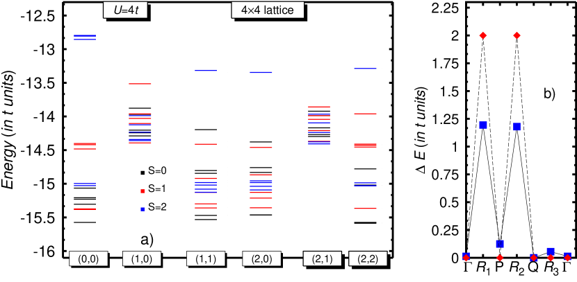
Figure 9: (Color online) The energy spectrum, obtained via Eq.(21), for the $4\times 4$ lattice with $N_{e}=14$ electrons at U=4t is shown in panel a). In panel b), the excitation energies from the ground state to the lowest-lying S=0,1, and S=2 states from panel a) are plotted as functions of the linear momentum quantum numbers $\Gamma=(0,0)$, $R_{1}=(1,0)$, $P=(2,0)$, $R_{2}=(2,1)$, $Q=(2,2)$, and $R_{3}=(1,1)$, respectively. In addition to U=4t (blue boxes), results for U=0t (red diamonds) are also included for comparison.

Coming back to the spectrum shown in panel a) of Fig.4, we note that the first excited state corresponds to a $\Theta=(1,2,2)$ configuration [with linear momenta $(\pi,\pi)$]. In fact, similar to the half-filled $2\times 4$ lattice, the first excited state for each combination $({\xi}_{x},{\xi}_{y})$ has spin S=1, exception made of $(0,0)$. The $2\times 4$ lattice displays a low-lying S=0 singlet (see Fig.1) while an S=2 quintet appears in the $4\times 4$ lattice. The excitation energies, referred to the ${\Theta}^{0}=(0,0,0)$ configuration, of these low-lying S=1 and S=2 states are shown in panel b) of Fig.4 as functions of the linear momentum quantum numbers. The shape of the curve does not fully agree with the one obtained with the spin-density wave (SDW) approximation Fawcett-sdw mainly due to the absence of degeneracy between the $\Gamma$=(0,0) and $Q$=(2,2) as well as the two peaks for the $R_{1}$=(1,0) and $R_{2}$=(2,1) points. Much of this discrepancy could, however, be due to finite size effects. Lanczos-Fano Note that the two peaks at $R_{1}$ and $R_{2}$, resulting from a kinetic-energy gap of 2t, are already visible for the Fermi gas (U=0t).

The DOS ${\cal{N}}(\omega)$ [Eq.(30)] for the half-filled $4\times 4$ lattice at U=4t is shown in panel a) of Fig.5. The calculations have been performed using $n_{T}$=5 HF-transformations along the lines described in Sec. II.3. In this case, Eqs.(24) and (28) provide us with 160 hole and particle solutions. A Lorentzian folding of width $\Gamma$=0.2t has been used. Similar to the case of the half-filled $2\times 4$ lattice, the Hubbard gap, $\Delta_{H}=U/2=2t$, remains present in this larger system. The hole (blue) and particle (black) spectral functions shown in panel b) of the figure show that the momenta $(\pm\pi/2,\pm\pi/2)$, $(0,\pi)$ and $(\pi,0)$ at the noninteracting Fermi surface have the largest spectral weight near $\omega$-U/2=0. Moreover, the spectral weight due to these momenta at the Fermi surface is particle-hole symmetric.

In panel a) of Fig.6, we have plotted the DOS ${\cal{N}}(\omega)$ [Eq.(30)] for the half-filled $4\times 4$ lattice at U=8t (i.e., an on-site repulsion equal to the noninteracting bandwidth W=8t) computed with $n_{T}$=5 HF-transformations. A Lorentzian folding of width $\Gamma$=0.2t has been used. The corresponding hole (blue) and particle (black) spectral functions are also displayed in panel b) of the figure. Our DOS and spectral functions [in particular, the ones corresponding to the linear momenta $(\pi,0)$, $(\pi/2,0)$ and $(0,0)$] can be compared with the ones, obtained using the Lanczos method, shown in Fig.2 of Ref. 57. As can be observed, the main qualitative features of the particle-hole symmetric DOS are well reproduced, namely the two prominent peaks at $\omega$-U/2 $\approx$ 2t and 3t (-2t and -3t) a lump peaked around $\omega$-U/2 $\approx$ 5t (-5t) and a smaller satellite peak in the neighborhood of $\omega$-U/2 $\approx$ 8t (-8t). In agreement with the results of Ref. 57, the upper and lower bands as well as the Hubbard gap are also clearly visible in Fig.6.

We have also studied the evolution of the DOS for the half-filled $4\times 4$ lattice as a function of U. To this end, in addition to the cases U=4t and 8t shown in Figs. 5 and 6, calculations have also been performed for U=2t, 12t and 20t. In good agreement with previous studies, Dagotto-RC-3184 ; moukouri2001 ; huscroft2001 ; aryanpour2003 ; stanescu2001 we observe that the Hubbard gap persists for increasing values of U. In our calculations, a pronounced suppression in the DOS around $\omega$-U/2=0 is observed with the DOS fully vanishing around U=8t (i.e., around the noninteracting bandwidth W=8t) which is precisely the region where a sizeable Hubbard gap is developed. Dagotto-RC-3184 ; Zgid ; stanescu2001

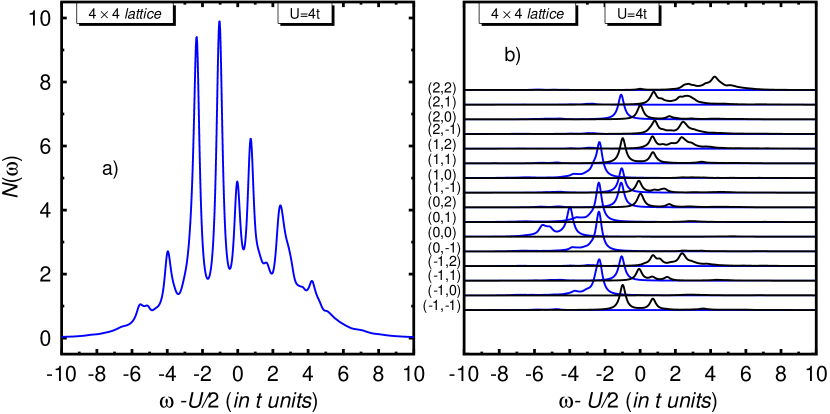
Figure 10: (Color online) The same as Fig.5 but for the $4\times 4$ lattice with $N_{e}$=14 electrons at U=4t.

Let us now consider two examples of a doped $4\times 4$ lattice. In Fig.7, we show the spectrum in the case of 15 electrons at U=4t. For each of the linear momentum quantum numbers (0,0), (1,0), (1,1), (2,0), (2,1) and (2,2), we plot the energies of the first five solutions of Eq.(21) for the spins S=1/2 and 3/2. The number of variational parameters in our approximation $n_{var}$($S=1/2,{\xi}_{x},{\xi}_{y})$=512 and $n_{var}$($S=3/2,{\xi}_{x},{\xi}_{y})$=516 should be compared with the dimensions $n_{RH}$($S=1/2,{\xi}_{x},{\xi}_{y})\approx$ 2 $\times 10^{6}$ and $n_{RH}$($S=3/2,{\xi}_{x},{\xi}_{y})\approx$ 2 $\times 10^{6}$ of the restricted Hilbert spaces. The first noticeable feature in Fig.7 is that the four-fold degenerate ${\Theta}^{-}=(1/2,1,1)$ ground state has non-zero linear momenta $(\pi/2,\pi/2)$. A finite linear momentum for the one-hole ground state has also been predicted in previous studies Dagotto-review using a variety of approximations for lattices of different sizes. Our numerical calculations also predict a two-fold degenerate (1/2,2,0) configuration whose energy is almost the same as the ground state one. For the noninteracting system (U=0t), the lowest-lying S=1/2 and S=3/2 states with linear momentum quantum numbers $\Gamma=(0,0)$, $P=(2,0)$, $Q=(2,2)$, and $R_{3}=(1,1)$ are degenerate and the same is also true for the configurations $R_{1}=(1,0)$ and $R_{2}=(2,1)$. Therefore, the huge degeneracy observed in the noninteracting case is already partially lifted at U=4t.

In Fig.8, we compare the ground state energy of the $4\times 4$ lattice with 15 electrons with the exact one Lanczos-Fano for U=4t. The energy -14.5469t predicted within our symmetry-projected configuration mixing approach, via Eq.(21), accounts for 99.19 $\%$ of the exact result. It is interesting to note that linear momentum plus $\hat{S}_{z}$ projection already accounts for 98.41 $\%$ of the exact solution. Nevertheless, full spin projection, while also recovering the total spin quantum number, still brings a sizeable amount of correlations.

The (shifted) differences ${\epsilon}_{1}^{{\Theta}^{0}}-{\epsilon}_{1}^{(1/2,{\xi}_{x},{\xi}_{y})}$-U/2, where ${\epsilon}_{1}^{{\Theta}^{0}}$ is the ground state energy of the half-filled lattice (Fig.4) and ${\epsilon}_{1}^{(1/2,{\xi}_{x},{\xi}_{y})}$ represents the energy of each of the lowest-lying S=1/2 states in Fig.7, compare very well with the position of the first prominent peak in the hole spectral functions shown in panel b) of Fig.5. For example, the variational approach predicts ${\epsilon}_{1}^{{\Theta}^{0}}-{\epsilon}_{1}^{(1/2,1,1)}$-U/2=-1.044t while the corresponding peak in the hole spectral function is predicted to be at $\omega$-U/2= -1.010t. The same is also true for the configuration with linear momenta ($\pi$,0) for which the variational approach predicts ${\epsilon}_{1}^{{\Theta}^{0}}-{\epsilon}_{1}^{(1/2,2,0)}$-U/2=-1.052t whereas the position of the corresponding peak in the hole spectral function is predicted to be at $\omega$-U/2= -1.012t. This leads to the conclusion that the lowest-lying S=1/2 states in the spectrum of Fig.7 are reasonably well described by a wave function of the form (23). This is remarkable, since no orbital relaxation is accounted for in this wave function, i.e., the determinants $|{\cal{D}}^{(i)}\rangle$ in Eq.(23) correspond to the ones obtained at half-filling.

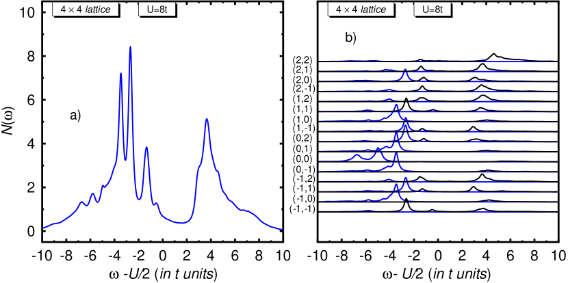
Figure 11: (Color online) The same as Fig.5 but for the $4\times 4$ lattice with $N_{e}$=14 electrons at U=8t. The shapes of the DOS as well as the spectral functions are qualitatively similar to the ones obtained using Lanczos calculations. Dagotto-RC-3184

The spectrum obtained, via Eq.(21), for 14 electrons at U=4t is displayed in Fig.9. The number of variational parameters in our approximation $n_{var}$($S=0,{\xi}_{x},{\xi}_{y})$=504, $n_{var}$($S=1,{\xi}_{x},{\xi}_{y})$=508 and $n_{var}$($S=2,{\xi}_{x},{\xi}_{y})$=512 should be compared with the dimensions $n_{RH}$($S=0,{\xi}_{x},{\xi}_{y})\approx 10^{6}$, $n_{RH}$($S=1,{\xi}_{x},{\xi}_{y})\approx 2\times 10^{6}$ and $n_{RH}$($S=2,{\xi}_{x},{\xi}_{y})\approx 10^{6}$ of the restricted Hilbert spaces. The ground state corresponds to the ${\Theta}^{0}$=(0,2,2) configuration [linear momenta ($\pi,\pi)$] with energy -15.5872t, while the exact one is -15.7446t. Lanczos-Fano On the other hand, the VMC approximation Ericprivate predicts a ground state energy of -15.5936t. Thus, both methods, ours and VMC, yield essentially the same relative error of around 1 $\%$ in the ground state energy per site. On the other hand, a relative error in the ground state energy per site of 0.45 $\%$ is obtained within the kDMRG approximation. Xiang

Our calculations also predict two other close-lying (0,2,2) solutions (with energies -15.5747t and -15.5777t) which cannot be distinguished in Fig.9 and therefore appear, together with the ground state, as a single thick black line. The energy -15.5743t of the ${\Theta}$=(0,0,0) configuration is also close to the actual ground state. As a result, the symmetry of the $\Gamma$ and $Q$ points is almost recovered in panel b) of Fig.9 where the energies of the lowest-lying S=0,1,2 states for each linear momentum combination are shown, referred to the ${\Theta}^{0}=(0,2,2)$ ground state for this system. Note that the configurations (0,1,1) and (0,2,0) (i.e., the points $R_{3}$ and $P$ in panel b) of Fig.9) have very small excitation energies, 0.0552t and 0.1242t, respectively. The two peaks at the points $R_{1}$ and $R_{2}$ are also present in the system with $N_{e}=14$ electrons at U=0t. The spectrum in panel a) of Fig.9 exhibits an increase in the density of energy levels, compared to the one at half-filling, pointing to its very correlated nature.

The DOS ${\cal{N}}(\omega)$ [Eq.(30)] for 14 electrons at U=4t is shown in panel a) of Fig.10. The calculations have been carried out by approximating the ($N_{e}$ $\pm$ 1)-electron systems with $n_{T}$=5 HF-transformations along the lines described in Sec. II.3. A Lorentzian folding of width $\Gamma$=0.2t has been used. The hole (blue) and particle (black) spectral functions are displayed in panel b) of the figure. In this case, Eqs.(24) and (28) provide us with 140 hole and 180 particle solutions. The chemical potential is now located around $\omega$-U/2=-1.2t. The comparison with panel b) of Fig.5 reveals that the structure of the hole states for $\omega$-U/2 $<$ -2t [i.e., those with linear momenta $(\pm\pi/2,0)$, $(0,\pm\pi/2)$ and $(0,0)$] remains to a large extent intact. On the other hand, a large fraction of the particle spectral weight observed at half-filling for 1t $<$ $\omega$-U/2 $<$ 3t is removed. This depletion occurs in favor of new states near $\omega$-U/2=0. The spectral decomposition of the DOS clearly shows that it is states around the Fermi surface that suffer the most pronounced changes with respect to half-filling. As a result, the particle-hole symmetry in the DOS, observed in Fig.5, is suppressed for this doped lattice and the original gap dissapears.

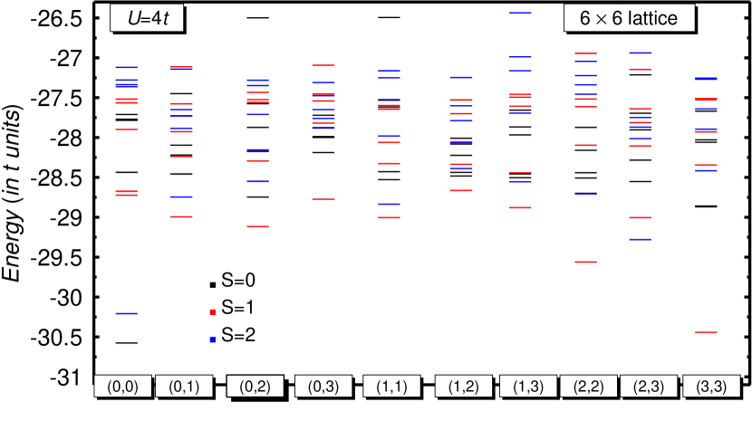
Figure 12: (Color online) The same as Fig.4 but for the half-filled $6\times 6$ lattice at U=4t.

In panel a) of Fig.11, we have plotted the DOS ${\cal{N}}(\omega)$ [Eq.(30)] for the $4\times 4$ lattice with 14 electrons at U=8t. The calculations were performed with $n_{T}$=5 HF-transformations and a folding $\Gamma$=0.2t has been used. The hole (blue) and particle (black) spectral functions are displayed in panel b) of the figure. Our DOS and spectral functions can be compared with the ones, obtained using the Lanczos method, shown in Figs.3 and 4 of Ref.57. The main qualitative features of the DOS are well reproduced, namely the prominent peaks around $\omega$-U/2=-4t, -3t, -2t and 4t. As can be noted from panel b) of Fig.11, the chemical potential is now located around $\omega$-U/2=-2.4t. One of the main features of the DOS is that it displays a pronounced pseudogap which, as can be seen from Figs. 6 and 11, results mainly from pulling particle strenghts into the (half-filling) gap combined with sizeable contributions of particle states around $\omega$-U/2=4t. We note, that the pseudogap problem in the doped 2D Hubbard model has also received attention within the framework of quantum cluster approaches. maier2005

We have also performed calculations for the $4\times 4$ lattice with 14 electrons at U=2t, 12t and 20t. From these calculations, and the results already discussed above for the cases U=4t and 8t, we conclude that upon dopping with two holes the original gap observed at half-filling dissapears for U=2t and 4t, a pseudogap is developed around the noninteracting bandwidth W=8t while for the larger interaction strengths U=12t and U=20t the gap is not filled. Similar conclusions have been obtained within the Lanczos framework. Dagotto-RC-3184

III.3 The square $6\times 6$ lattice

Finally, let us turn our attention to the half-filled $6\times 6$ lattice at U=4t. The dimensions $n_{RH}$($S=0,{\xi}_{x},{\xi}_{y})\approx 2\times 10^{17}$, $n_{RH}$($S=1,{\xi}_{x},{\xi}_{y})\approx 6\times 10^{17}$ and $n_{RH}$($S=2,{\xi}_{x},{\xi}_{y})\approx 6\times 10^{17}$ of the corresponding restricted Hilbert spaces are far too large for a brute force diagonalization to be feasible. Other approximate methods are then called for, not only to describe ground state properties but also to access the excitation spectrum in this relatively large lattice for which information is rather scarce. In this case, the number of variational parameters in our approximation is $n_{var}$($S=0,{\xi}_{x},{\xi}_{y})$=2592, $n_{var}$($S=1,{\xi}_{x},{\xi}_{y})$=2596 and $n_{var}$($S=2,{\xi}_{x},{\xi}_{y})$=2600, respectively. Therefore, the half-filled $6\times 6$ lattice represents a very challenging testing ground for our symmetry-projected configuration mixing approximation.

In Fig.12, we show the energies ${\epsilon}_{\alpha}^{\Theta}$ obtained, via Eq.(21), for the ten essentially different pairs of linear momentum quantum numbers (0,0), (0,1), (0,2), (0,3), (1,1), (1,2), (1,3), (2,2), (2,3) and (3,3). For each of them we have plotted the first five solutions with spins S=0,1, and 2. The ground state corresponds to the ${\Theta}^{0}$=(0,0,0) configuration with energy ${\epsilon}_{1}^{{\Theta}^{0}}$=-30.5766t. This can be compared with the energy obtained using state-of-the-art auxiliary-field MC, -30.89(1)t. Shiweiprivate

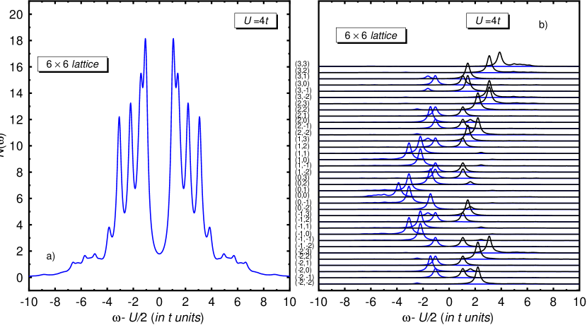
Figure 13: (Color online) The same as Fig.5 but for the half-filled $6\times 6$ lattice at U=4t.

From Fig.12, we realize that the first excited state corresponds to a $\Theta=(1,3,3)$ configuration [with linear momenta $(\pi,\pi)$]. The energy difference 0.1331t between this $(\pi,\pi)$-configuration and the ground state is smaller than the corresponding value 0.1651t for the half-filled $4\times 4$ system. On the other hand, similar to the half-filled $2\times 4$ and $4\times 4$ lattices, most of the first excited states for each combination $({\xi}_{x},{\xi}_{y})$ have spin S=1, exception made of $(0,0)$ and $(2,3)$ for which an S=2 quintet appears. Note that our calculations predict the lowest-lying (1,0,1), (1,1,1) and (1,2,3) solutions to be quite close in energy. As with the other half-filled lattices studied, we find only a handful of excited states within an energy window of t from the ground state.

The DOS ${\cal{N}}(\omega)$ [Eq.(30)] for the half-filled $6\times 6$ lattice at U=4t is shown in panel a) of Fig.13. The calculations have been carried out with $n_{T}$=5 HF-transformations along the lines described in Sec. II.3. In this case, Eqs.(24) and (28) provide us with 360 hole and particle solutions. A Lorentzian folding of width $\Gamma$=0.2t has been used. The DOS for this large lattice shows a clear Hubbard gap $\Delta_{H}=U/2=2t$. The fact that the gap remains intact in going, at half-filling, from the $4\times 4$ to the $6\times 6$ lattice is consistent with previous studies within the DCA which show that it is preserved even in the TDL. moukouri2001 ; huscroft2001 ; aryanpour2003 We note, that the DMFT (i.e., $N_{c}=1$) does not predict a gap for U=4t. It is only for a larger number $N_{c}$ of clusters that the gap starts to develop in these studies at the TDL. maier2005 Back to our DOS, we see again from the spectral decomposition, shown in panel b) of Fig.13, that it is states at [i.e., $(\pm 2\pi/3,\pm\pi/3)$, $(\pm\pi/3,\pm 2\pi/3)$, $(\pi,0)$ and $(0,\pi)$] or close to the noninteracting Fermi surface that contribute the largest spectral weight to the prominent hole and particle peaks around $\omega$-U/2=-t and $\omega$-U/2=t. In general, the DOS for this finite size lattice is still highly peaked, though features should smooth out as one approaches the TDL. Systematic studies for the $8\times 8$ and $10\times 10$ lattices are in progress and will be presented elsewhere.

IV Conclusions

How to accurately describe many-fermion systems with approximate methods, which truncate the complete expansion of the wave functions to a numerically feasible number of configurations, is a central question in nuclear structure theory, quantum chemistry, and condensed matter physics. To this end, in the present study we have explored an alternative avenue for the 2D Hubbard model. The main accomplishments of the present study are:

• We have presented a powerful methodology of a VAP configuration mixing scheme, originally devised for the nuclear many-body problem, but not yet used to study ground and excited states, with well defined quantum numbers, of the 2D Hubbard model with nearest-neighbor hopping and PBC.

Our scheme relies on the Ritz variational principle to construct, throughout a chain of VAP calculations, a truncated basis consisting of a few (orthonormalized) symmetry-projected HF states. The simple structure of the projected wave functions employed, combined with a fast minimization algorithm, allows to keep low computational cost in building our basis. A further diagonalization of the Hamiltonian within such a basis allows to account, in a similar fashion, for residual correlations in the ground and excited states.

• Due to the simple structure of the wave functions in our approximation, we can construct an ansatz [Eqs. (23 ) and (27)], whose flexibility is well-controlled by the number of HF-transformations included, to approximate the ground state of the $(N_{e}\pm 1)$-electron system. This allows us to determine one-electron affinities and ionization potentials as well as to access the spectral weight of states with different linear momentum quantum numbers in the calculation of spectral functions and the corresponding density of states.

• We have shown that our approximation gives accurate results, as compared with exact energies, for the $2\times 4$ and $4\times 4$ lattices. We have also provided the low-lying spectrum of the $6\times 6$ lattice which, to the best of our knowledge, has not been reported in the literature. Our ground state energy for this lattice compares well with results from state-of-the-art auxiliary-field Monte Carlo calculations.

Regarding the physics of the 2D Hubbard model, we have discussed the trends, in going from the $2\times 4$ to the $4\times 4$ and $6\times 6$ half-filled lattices, of both the low-lying spectra and the spectral functions as well as the corresponding density of states. We have found that the ground states correspond to configurations with spin zero and linear momenta (0,0). We have also found that most of the lowest-lying excited states display spin S=1. The doped systems with 14 and 15 electrons in the $4\times 4$ lattice have also been considered. The ground states of such systems correspond to configurations with linear momenta different from zero.

Special attention has been paid to the spectral weight of states with different linear momentum quantum numbers. We have compared the DOS predicted within our approximation with the one obtained using an exact diagonalization for the half-filled $2\times 4$ lattice and found an excellent agreement between the two. Our results for the half-filled $4\times 4$ lattice, at different on-site repulsions, agree qualitatively well with the ones obtained using the Lanczos method. Dagotto-RC-3184 For all the considered half-filled lattices, a Hubbard gap is predicted within our approximation. In particular, the fact that this gap persists in going from the $4\times 4$ to the $6\times 6$ system is consistent with previous studies within cluster extensions to dynamical mean field theory which show that it is preserved even in the thermodynamic limit. As opposed to the half-filled case, the particle-hole symmetry in the DOS is removed when doping is present in the system. From the calculations for 14 electrons in the $4\times 4$ lattice we conclude that for on-site repulsions smaller than the noninteracting bandwidth the (half-filling) gap dissapears, a pseudogap develops around U=8t while the gap is not filled for larger U values. These results agree well with similar conclusions extracted from Lanczos calculations. Dagotto-RC-3184 We have also found the remarkable result that all the lowest-lying S=1/2 states in the spectrum of the $4\times 4$ lattice with 15 electrons can be reasonably well described by a wave function of the form (23) in which no orbital relaxation is accounted for.

One important feature of the scheme presented in this study is that it leaves ample space for further improvements and research. First, the number of symmetry-projected configurations in our basis set can be easily increased. Second, we could still incorporate particle number symmetry breaking and restoration in our configuration mixing scheme to access even more correlations. Our methods could be useful even for more complicated lattices like the honeycomb one. An extension of the considered 2D t-U Hubbard Hamiltonian to the $t-t^{{}^{\prime}}-t^{{}^{\prime\prime}}-U$ case is also straightforward, allowing the study of several interesting issues like indications of spin-charge separation in 2D systems (see, for example, Ref. 65 and references therein). Last but not least, not only the configuration mixing scheme applied in the present work but also the full hierarchy of approximations discussed in Ref. 43 can be implemented for the molecular Hamiltonian in the realm of quantum chemistry, within the already successful PQT. PQT-reference-1 ; PQT-reference-2 Work along these avenues is in progress.

We would like to stress that the cost of the symmetry-projected calculations described in this work has the same scaling as mean-field methods. PQT-reference-1 ; PQT-reference-2 This statement is true as long as the number of grid points required in the symmetry restoration remains relatively constant (this is usually the case for spin and number projection). Note, however, that the restoration of translational symmetry in Hubbard lattices with PBC requires a number of grid points equal to $N_{sites}$. This makes the cost of our calculations ${\cal{O}}(N_{sites})$ more expensive than the Hartree-Fock method, which is still a very reasonable scaling. The computational effort is mainly concentrated in looping over grid points for the evaluation of matrix elements. This task is trivially parallelizable and one can thus easily reach clusters larger than the ones considered in this study. Preliminary calculations for the half-filled and doped $8\times 8$ and $10\times 10$ lattices are in progress.

A discussion of the limitations of our method is also in order here. Evidently, our method relies on the Hamiltonian having good symmetries. The lower the number of symmetries of a given Hamiltonian, the lower the correlations that can be accounted for by means of symmetry restoration. On the other hand, the most interesting quantum behavior is found in systems where symmetries are present. Second, it is known that the correlation energy per particle obtained with approaches based on a single symmetry-projected determinant PQT-reference-1 ; PQT-reference-2 decays as the lattice size increases. We observe that the error in the energy per site is larger in the case of the half-filled $6\times 6$ lattice than in the $4\times 4$ one, although in both cases we have restricted the present study to $m$=5 transformations. One can, however, increase the number of transformations to maintain the quality of our wave functions. In principle, if the number of transformations is equal to the size of the restricted Hilbert subspace the method becomes exact. In practice, one can only hope that the number of transformations needed to access the relevant physics of the considered lattices is relatively low.

Finally, we believe that the finite size calculations discussed in the present work are complementary to other approaches where impurity solvers play an important role. However, the symmetries to be broken and restored in the impurity-bath and bath Hamiltonians will depend on the details of the case considered. Zgid

Appendix A Symmetry-projected matrix elements between two Slater determinants $|{\cal{D}}^{i}\rangle$ and $|{\cal{D}}^{k}\rangle$

In this appendix, we present the expressions for the matrix elements ${\cal{H}}_{\Sigma{\Sigma}^{{}^{\prime}}}^{ik\Theta}=\langle{\cal{D}}^{i}|\hat{H}_{Hub}\hat{P}_{\Sigma{\Sigma}^{{}^{\prime}}}^{\Theta}|{\cal{D}}^{k}\rangle$ and ${\cal{N}}_{\Sigma{\Sigma}^{{}^{\prime}}}^{ik\Theta}=\langle{\cal{D}}^{i}|\hat{P}_{\Sigma{\Sigma}^{{}^{\prime}}}^{\Theta}|{\cal{D}}^{k}\rangle$ required to compute the kernels ${\cal{H}}_{\Sigma{\Sigma}^{{}^{\prime}}}^{m\Theta}$ and ${\cal{N}}_{\Sigma{\Sigma}^{{}^{\prime}}}^{m\Theta}$ in Eq.(20) of Sec. II.2. Note that the matrix elements required in Eq.(8) of Sec. II.1 are just a particular case where both Slater determinants are the same. Here, and in what follows, we keep our notation as close as possible to the one already used for the 1D Hubbard model. Carlos-Hubbard-1D Both ${\cal{H}}_{\Sigma{\Sigma}^{{}^{\prime}}}^{ik\Theta}$ and ${\cal{N}}_{\Sigma{\Sigma}^{{}^{\prime}}}^{ik\Theta}$ read

$${\cal{H}}_{\Sigma{\Sigma}^{{}^{\prime}}}^{ik\Theta} = \frac{2S+1}{8{\pi}^{2}N_{sites}}\sum_{{\bf{j}}}e^{-i{\bf{k}}_{\xi}{\bf{j}}}\int d\Omega D_{\Sigma{\Sigma}^{{}^{\prime}}}^{S*}(\Omega)h^{ik}(\Omega,{\bf{j}})n^{ik}(\Omega,{\bf{j}})$$

$${\cal{N}}_{\Sigma{\Sigma}^{{}^{\prime}}}^{ik\Theta} = \frac{2S+1}{8{\pi}^{2}N_{sites}}\sum_{{\bf{j}}}e^{-i\bf{k}_{\xi}\bf{j}}\int d\Omega D_{\Sigma{\Sigma}^{{}^{\prime}}}^{S*}(\Omega)n^{ik}(\Omega,{\bf{j}})$$ (31)

where, ${\bf{k}}_{\xi}=\left(k_{{\xi}_{x}},k_{{\xi}_{y}}\right)=\left(\frac{2\pi{\xi}_{x}}{N_{x}},\frac{2\pi{\xi}_{y}}{N_{y}}\right)$ and ${\bf{j}}=\left(j_{x},j_{y}\right)$, respectively. For the gauge-rotated norm

$$n^{ik}(\Omega,{\bf{j}})=det_{N_{e}}{\cal{X}}^{ik}(\Omega,{\bf{j}})$$ (32)

the determinant has to be taken over the $N_{e}\times N_{e}$ dimensional occupied part of the matrix

$${\cal{X}}_{ab}^{ik}(\Omega,{\bf{j}})=\left({\cal{D}}^{iT}{\cal{S}}(\Omega,{\bf{j}}){\cal{D}}^{k*}\right)_{ab}$$ (33)

with

$${\cal{S}}_{{\boldsymbol{\alpha}}\sigma{\sigma}^{{}^{\prime}}}(\Omega,{\bf{j}})={\cal{D}}_{\sigma{\sigma}^{{}^{\prime}}}^{1/2}(\Omega)e^{i{\bf{k}}_{\alpha}{\bf{j}}}$$ (34)

The gauge-rotated Hamiltonian takes the form

$$h^{ik}(\Omega,{\bf{j}})=\frac{1}{2}t^{ik}(\Omega,{\bf{j}})+\frac{1}{2}Tr\left({\Gamma}^{ik}(\Omega,{\bf{j}}){\rho}^{ki}(\Omega,{\bf{j}})\right)$$ (35)

with

$$t^{ik}(\Omega,{\bf{j}}) =\sum_{{\boldsymbol{\alpha}}{\sigma}}\epsilon({\bf{k}}_{\alpha}){\rho}_{{\boldsymbol{\alpha}}{\sigma},{\boldsymbol{\alpha}}{\sigma}}^{ki}(\Omega,{\bf{j}})$$

$$\epsilon({\bf{k}}_{\alpha}) =-2t\left(cosk_{{\alpha}_{x}}+cosk_{{\alpha}_{y}}\right)$$

$${\rho}_{{\boldsymbol{\gamma}}{\sigma}^{{}^{\prime}},{\boldsymbol{\alpha}}\sigma}^{ki}(\Omega,{\bf{j}}) =\sum_{{\sigma}^{"}hh^{{}^{\prime}}}{\cal{S}}_{{\boldsymbol{\gamma}}{\sigma}^{{}^{\prime}}{\sigma}^{"}}(\Omega,{\bf{j}}){\cal{D}}_{{\boldsymbol{\gamma}}{\sigma}^{"},h}^{k*}\Big{[}{\cal{X}}_{hh^{{}^{\prime}}}^{ik}(\Omega,{\bf{j}})\Big{]}^{-1}{\cal{D}}_{{\boldsymbol{\alpha}}\sigma,h^{{}^{\prime}}}^{i}$$

$${\Gamma}_{{\boldsymbol{\alpha}}\sigma,{\boldsymbol{\gamma}}{\sigma}^{{}^{\prime}}}^{ik}(\Omega,{\bf{j}}) ={\delta}_{\sigma{\sigma}^{{}^{\prime}}}{\delta}_{{\alpha}_{x}{\gamma}_{x}}{\delta}_{{\alpha}_{y}{\gamma}_{y}}\epsilon({\bf{k}}_{\alpha})+\frac{U}{N_{sites}}\sum_{{\boldsymbol{\beta}}{\boldsymbol{\delta}}}{\delta}_{{\alpha}_{x}+{\beta}_{x}-{\gamma}_{x}-{\delta}_{x}}^{0,\pm N_{x}}{\delta}_{{\alpha}_{y}+{\beta}_{y}-{\gamma}_{y}-{\delta}_{y}}^{0,\pm N_{y}}\times$$

$$\times\Big{[}{\delta}_{\sigma{\sigma}^{{}^{\prime}}}{\rho}_{{\boldsymbol{\delta}}-\sigma,{\boldsymbol{\beta}}-\sigma}^{ki}(\Omega,{\bf{j}})-\left(1-{\delta}_{\sigma{\sigma}^{{}^{\prime}}}\right){\rho}_{{\boldsymbol{\delta}}\sigma,{\boldsymbol{\beta}}-\sigma}^{ki}(\Omega,{\bf{j}})\Big{]}$$ (36)

where the product of generalized Kronecker deltas in ${\Gamma}^{ik}(\Omega,{\bf{j}})$ results from the transformation of the on-site interaction term in Eq.(1) to the momentum representation. As a consequence of the PBC, ${\delta}_{{\alpha}_{i}+{\beta}_{i}-{\gamma}_{i}-{\delta}_{i}}^{0;\pm N_{i}}$ is one if ${\alpha}_{i}+{\beta}_{i}-{\gamma}_{i}-{\delta}_{i}$ is either 0 or $\pm N_{i}$ and zero else.

Appendix B Symmetry-projected particle-hole matrix elements between two Slater determinants $|{\cal{D}}^{i}\rangle$ and $|{\cal{D}}^{k}\rangle$

In this appendix, we present the expressions for the matrix elements ${\cal{H}}_{\Sigma{\Sigma}^{{}^{\prime}}}^{ik\Theta;ph}=\langle{\cal{D}}^{i}|\hat{H}_{Hub}\hat{P}_{\Sigma{\Sigma}^{{}^{\prime}}}^{\Theta}{\hat{b}}^{\dagger}_{p}({\cal{D}}^{k}){\hat{b}}_{h}({\cal{D}}^{k})|{\cal{D}}^{k}\rangle$ and ${\cal{N}}_{\Sigma{\Sigma}^{{}^{\prime}}}^{ik\Theta;ph}=\langle{\cal{D}}^{i}|\hat{P}_{\Sigma{\Sigma}^{{}^{\prime}}}^{\Theta}{\hat{b}}^{\dagger}_{p}({\cal{D}}^{k}){\hat{b}}_{h}({\cal{D}}^{k})|{\cal{D}}^{k}\rangle$ required to compute the kernels ${\cal{K}}_{\Sigma{\Sigma}^{{}^{\prime}}}^{m\Theta;ph}$ and ${\cal{R}}_{\Sigma{\Sigma}^{{}^{\prime}}}^{m\Theta;ph}$ defining the variational equations discussed in Sec. II.2. Note that the matrix elements required in Eq.(10) of Sec. II.1 are just a particular case where both Slater determinants are the same. We obtain

$${\cal{H}}_{\Sigma{\Sigma}^{{}^{\prime}}}^{ik\Theta;ph} = \frac{2S+1}{8{\pi}^{2}N_{sites}}\sum_{{\bf{j}}}e^{-i{\bf{k}}_{\xi}{\bf{j}}}\int d\Omega D_{\Sigma{\Sigma}^{{}^{\prime}}}^{S*}(\Omega)n^{ik}(\Omega,{\bf{j}})h_{ph}^{ik}(\Omega,{\bf{j}})$$

$${\cal{N}}_{\Sigma{\Sigma}^{{}^{\prime}}}^{ik\Theta;ph} = \frac{2S+1}{8{\pi}^{2}N_{sites}}\sum_{{\bf{j}}}e^{-i{\bf{k}}_{\xi}{\bf{j}}}\int d\Omega D_{\Sigma{\Sigma}^{{}^{\prime}}}^{S*}(\Omega)n^{ik}(\Omega,{\bf{j}})n_{ph}^{ik}(\Omega,{\bf{j}})$$ (37)

where, as in appendix A, ${\bf{k}}_{\xi}=\left(k_{{\xi}_{x}},k_{{\xi}_{y}}\right)=\left(\frac{2\pi{\xi}_{x}}{N_{x}},\frac{2\pi{\xi}_{y}}{N_{y}}\right)$ and ${\bf{j}}=\left(j_{x},j_{y}\right)$, respectively. On the other hand,

$$n_{ph}^{ik}(\Omega,{\bf{j}})=\sum_{h{{}^{\prime}}\in{\cal{D}}^{(i)}}\Big{[}{\cal{X}}_{hh^{{}^{\prime}}}^{ik}(\Omega,{\bf{j}})\Big{]}^{-1}{\cal{X}}_{h^{{}^{\prime}}p}^{ik}(\Omega,{\bf{j}})$$ (38)

with the indices $h$ ($p$) running over all the occupied (unoccupied) states in $|{\cal{D}}^{k}\rangle$. The inverse $\Big{[}{\cal{X}}_{hh^{{}^{\prime}}}^{ik}(\Omega,{\bf{j}})\Big{]}^{-1}$ is taken over the occupied part of the matrix (33). Finally,

$$h_{ph}^{ik}(\Omega,{\bf{j}}) = n_{ph}^{ik}(\Omega,{\bf{j}})h^{ik}(\Omega,{\bf{j}})+\Big{[}{\cal{Y}}^{ki}(\Omega,{\bf{j}}){\Gamma}^{ik}(\Omega,{\bf{j}}){\overline{\cal{W}}}^{ki}(\Omega,{\bf{j}})\Big{]}_{hp}$$ (39)

with the functions ${\cal{Y}}(\Omega,{\bf{j}})$ and ${\overline{\cal{W}}}^{ki}(\Omega,{\bf{j}})$) defined, for all the occupied $h$ and unoccupied $p$ states in $|{\cal{D}}^{k}\rangle$, as

$${\cal{Y}}_{h,{\boldsymbol{\alpha}}\sigma}^{ki}(\Omega,{\bf{j}}) = \sum_{h^{{}^{\prime}}}\Big{[}{\cal{X}}_{hh^{{}^{\prime}}}^{ik}(\Omega,{\bf{j}})\Big{]}^{-1}{\cal{D}}_{{\boldsymbol{\alpha}}\sigma,h^{{}^{\prime}}}^{i}$$

$${\overline{\cal{W}}}_{{\boldsymbol{\gamma}}{\sigma}^{{}^{\prime}},p}^{ki}(\Omega,{\bf{j}}) = \sum_{{\boldsymbol{\delta}}{\sigma}^{"}{\sigma}^{{}^{\prime\prime\prime}}}\Big{[}1-{\rho}^{ki}(\Omega,{\bf{j}})\Big{]}_{{\boldsymbol{\gamma}}{\sigma}^{{}^{\prime}},{\boldsymbol{\delta}}{\sigma}^{"}}{\cal{S}}_{{\boldsymbol{\delta}}{\sigma}^{"}{\sigma}^{{}^{\prime\prime\prime}}}(\Omega,{\bf{j}}){\cal{D}}_{{\boldsymbol{\delta}}{\sigma}^{{}^{\prime\prime\prime}},p}^{k*}$$ (40)

Appendix C Symmetry-projected matrix elements between two Slater determinants $|{\cal{D}}^{i}\rangle$ and $|{\cal{D}}^{k}\rangle$ for spectral functions

In this appendix, we present the computation of the kernels ${\cal{H}}^{{\Theta}^{-}}$ and ${\cal{N}}^{{\Theta}^{-}}$ required in Eq.(24) as well as of the kernels ${\cal{H}}^{{\Theta}^{+}}$ and ${\cal{N}}^{{\Theta}^{+}}$ in Eq.(28). Both ${\cal{H}}^{{\Theta}^{-}}$ and ${\cal{N}}^{{\Theta}^{-}}$ read

$${\cal{N}}_{ih\sigma;kh^{{}^{\prime}}{\sigma}^{{}^{\prime}}}^{{\Theta}^{-}} = \frac{2}{8{\pi}^{2}N_{sites}}\sum_{{\bf{j}}}e^{-i{\bf{k}}_{\xi}{\bf{j}}}\int d\Omega D_{\sigma{\sigma}^{{}^{\prime}}}^{1/2*}(\Omega)n^{ik}(\Omega,{\bf{j}})n_{hh^{{}^{\prime}}}^{ik}(\Omega,{\bf{j}})$$

$${\cal{H}}_{ih\sigma;kh^{{}^{\prime}}{\sigma}^{{}^{\prime}}}^{{\Theta}^{-}} = \frac{2}{8{\pi}^{2}N_{sites}}\sum_{{\bf{j}}}e^{-i{\bf{k}}_{\xi}{\bf{j}}}\int d\Omega D_{\sigma{\sigma}^{{}^{\prime}}}^{1/2*}(\Omega)n^{ik}(\Omega,{\bf{j}})h_{hh^{{}^{\prime}}}^{ik}(\Omega,{\bf{j}})$$ (41)

with the vector ${\bf{k}}_{\xi}=\left(k_{{\xi}_{x}^{-}},k_{{\xi}_{y}^{-}}\right)=\left(\frac{2\pi{\xi}_{x}^{-}}{N_{x}},\frac{2\pi{\xi}_{y}^{-}}{N_{y}}\right)$ while i,k = 1, $\dots$ $n_{T}$, $h,h^{{}^{\prime}}=1,\dots N_{e}$ and $\sigma,{\sigma}^{{}^{\prime}}=\pm 1/2$. On the other hand

$$n_{hh^{{}^{\prime}}}^{ik}(\Omega,{\bf{j}})=\Big{[}{\cal{X}}_{h^{{}^{\prime}}h}^{ik}(\Omega,{\bf{j}})\Big{]}^{-1}$$ (42)

and

$$h_{hh^{{}^{\prime}}}^{ik}(\Omega,{\bf{j}})=\Big{[}{\cal{X}}_{h^{{}^{\prime}}h}^{ik}(\Omega,{\bf{j}})\Big{]}^{-1}h^{ik}(\Omega,{\bf{j}})-\Big{[}{\cal{Y}}^{ki}(\Omega,{\bf{j}}){\Gamma}^{ik}(\Omega,{\bf{j}}){\cal{Z}}^{ki}(\Omega,{\bf{j}})\Big{]}_{h^{{}^{\prime}}h}$$ (43)

respectively. The function ${\cal{Z}}_{{\boldsymbol{\gamma}}{\sigma}^{{}^{\prime}},h}^{ki}(\Omega,{\bf{j}})$ reads

$${\cal{Z}}_{{\boldsymbol{\gamma}}{\sigma}^{{}^{\prime}},h}^{ki}(\Omega,{\bf{j}})=\sum_{h^{"}\sigma^{"}}S_{{\boldsymbol{\gamma}}{\sigma}^{{}^{\prime}}{\sigma}^{"}}(\Omega,{\bf{j}})D_{{\boldsymbol{\gamma}}{\sigma}^{"},h^{"}}^{k*}\Big{[}{\cal{X}}_{h^{"}h}^{ik}(\Omega,{\bf{j}})\Big{]}^{-1}$$ (44)

while ${\cal{Y}}_{h^{{}^{\prime}},{\boldsymbol{\alpha}}\sigma}^{ki}(\Omega,{\bf{j}})$ is given in Eq.(B).

The norm and Hamiltonian overlaps in Eq.(28) read

$${\cal{N}}_{ip\sigma,kp^{{}^{\prime}}{\sigma}^{{}^{\prime}}}^{{\Theta}_{+}} = \frac{2}{8{\pi}^{2}N_{sites}}\sum_{{\bf{j}}}e^{-i{\bf{k}}_{\xi}{\bf{j}}}\int d\Omega D_{\sigma{\sigma}^{{}^{\prime}}}^{1/2*}(\Omega)n^{ik}(\Omega,{\bf{j}})n_{pp^{{}^{\prime}}}^{ik}(\Omega,{\bf{j}})$$

$${\cal{H}}_{ip\sigma,kp^{{}^{\prime}}{\sigma}^{{}^{\prime}}}^{{\Theta}_{+}} = \frac{2}{8{\pi}^{2}N_{sites}}\sum_{{\bf{j}}}e^{-i{\bf{k}}_{\xi}{\bf{j}}}\int d\Omega D_{\sigma{\sigma}^{{}^{\prime}}}^{1/2*}(\Omega)n^{ik}(\Omega,{\bf{j}})h_{pp^{{}^{\prime}}}^{ik}(\Omega,{\bf{j}})$$ (45)

with the vector ${\bf{k}}_{\xi}=\left(k_{{\xi}_{x}^{+}},k_{{\xi}_{y}^{+}}\right)=\left(\frac{2\pi{\xi}_{x}^{+}}{N_{x}},\frac{2\pi{\xi}_{y}^{+}}{N_{y}}\right)$ while i,k = 1, $\dots$ $n_{T}$, $p,p^{{}^{\prime}}=N_{e}+1,\dots 2N_{sites}$ and $\sigma,{\sigma}^{{}^{\prime}}=\pm 1/2$. On the other hand,

$$n_{pp^{{}^{\prime}}}^{ik}(\Omega,{\bf{j}})={\cal{X}}_{pp^{{}^{\prime}}}^{ik}(\Omega,{\bf{j}})-\sum_{hh^{{}^{\prime}}}{\cal{X}}_{ph}^{ik}(\Omega,{\bf{j}})\Big{[}{\cal{X}}_{hh^{{}^{\prime}}}^{ik}(\Omega,{\bf{j}})\Big{]}^{-1}{\cal{X}}_{h^{{}^{\prime}}p^{{}^{\prime}}}^{ik}(\Omega,{\bf{j}})$$ (46)

and

$$h_{pp^{{}^{\prime}}}^{ik}(\Omega,{\bf{j}}) = n_{pp^{{}^{\prime}}}^{ik}(\Omega,{\bf{j}})h^{ik}(\Omega,{\bf{j}})+\Big{[}{\cal{W}}^{ik}(\Omega,{\bf{j}}){\Gamma}^{ik}(\Omega,{\bf{j}}){\overline{\cal{W}}}^{ki}(\Omega,{\bf{j}})\Big{]}_{pp^{{}^{\prime}}}$$ (47)

respectively. The function ${\cal{W}}_{p,{\boldsymbol{\alpha}}\sigma}^{ik}(\Omega,{\bf{j}})$ is given by

$${\cal{W}}_{p,{\boldsymbol{\alpha}}\sigma}^{ik}(\Omega,{\bf{j}})=\sum_{{\boldsymbol{\beta}}{\sigma}^{{}^{\prime}}}{\cal{D}}^{i}_{{\boldsymbol{\beta}}{\sigma}^{{}^{\prime}},p}\Big{[}1-{\overline{\rho}}^{ki}(\Omega,{\bf{j}})\Big{]}_{{\boldsymbol{\beta}}{\sigma}^{{}^{\prime}},{\boldsymbol{\alpha}}\sigma}$$ (48)

while ${\overline{\cal{W}}}_{{\boldsymbol{\gamma}}{\sigma}^{{}^{\prime}},p^{{}^{\prime}}}^{ki}(\Omega,{\bf{j}})$ is defined in Eq.(B).

References

- (1) J. G. Bednorz and K. A. Müller, Z. Phys. B 64, 189 (1986).
- (2) E. Dagotto, Rev. Mod. Phys. 66, 763 (1994).
- (3) J. Hubbard, Proc. R. Soc. (London) A 276, 238 (1963).
- (4) P. W. Anderson, Science 235, 1196 (1987).
- (5) R. Jördens, N. Strohmaier, K. Günter, H. Moritz and T. Esslinger, Nature 455, 204 (2008).
- (6) U. Schneider, L. Hackermüller, S. Will, Th. Best, I. Bloch, T. A. Costi, R. W. Helmes, D. Rasch and A. Rosch, Science 322, 1520 (2008).
- (7) I. Bloch, J. Dalibard and W. Zwerger, Rev. Mod. Phys. 80, 885 (2008).
- (8) A. H. Castro Neto, F. Guinea, N. M. R. Peres, K., S. Novosolev and A. K. Geim, Rev. Mod. Phys. 81, 109 (2009).
- (9) F. Gebhard, The Mott Metal-Insulator Transition (Springer, Berlin, 1997).
- (10) Y. Nagaoka, Phys. Rev. 147, 392 (1967).
- (11) E. Dagotto and J. R. Schrieffer, Phys. Rev. B 43, 8705 (1991).
- (12) C. -C. Chang and S. Zhang, Phys. Rev. Lett. 104, 116402 (2010).
- (13) C. -C. Chang and S. Zhang, Phys. Rev. B 78, 165101 (2008).
- (14) F. H. L. Essler, H. Frahm, F. Göhmann, A. Klümper and V. E. Korepin, The One-Dimensional Hubbard Model (University Press, Cambridge, 2005).
- (15) K. J. von Szczepanski, P. Horsch, W. Stephan and M. Ziegler, Phys. Rev. B 41, 2017 (1990).
- (16) E. Manousakis, Rev. Mod. Phys. 63, 1 (1991).
- (17) G. Fano, F. Ortolani and A. Parola, Phys. Rev. B 46, 1048 (1992); 42, 6877 (1990).
- (18) Quantum Monte Carlo Methods in Physics and Chemistry edited by M. P. Nightingale and C. J. Umrigar, NATO Advanced Studies Institute, Series C: Mathematical and Physical Sciences (Kluwer, Dordrecht, 1999), Vol. 525.
- (19) H. De Raedt and W. von der Linden, The Monte Carlo Method in Condensed Matter Physics, edited by K. Binder (Springer-Verlag, Heidelberg, 1992).
- (20) S. Sorella, Phys. Rev. B 84, 241110 (2011).
- (21) S. R. White, Phys. Rev. Lett. 69, 2863 (1992).
- (22) J. Dukelsky and S. Pittel, Rep. Prog. Phys. 67, 513 (2004).
- (23) U. Schollwöck, Rev. Mod. Phys. 77, 259 (2005).
- (24) U. Schollwöck, Ann. Phys. 326, 96 (2011).
- (25) G. K. -L. Chan and S. Sharma, Ann. Rev. Phys. Chem. 62, 465 (2011).
- (26) F. Verstraete, V. Murg and J. I. Cirac, Adv. Phys. 57, 143 (2008).
- (27) L. Tagliacozzo, G. Evenbly and G. Vidal, Phys. Rev. B 80, 235127 (2009).
- (28) C. V. Kraus, N. Schuch, F. Verstraete and J. I. Cirac, Phys. Rev. A 81, 052338 (2010).
- (29) Z. Gu, preprint ArXiv/cond-mat.str-el: 1109.4470v1 (2011).
- (30) J. M. Luttinger and J. C. Ward, Phys. Rev. 118, 1417 (1960).
- (31) M. Potthoff, Eur. Phys. J. B 32, 429 (2003).
- (32) A. L. Fetter and J. D. Walecka, Quantum Theory of Many-Particle systems (McGraw-Hill, New York, 1971).
- (33) M. Balzer, W. Hanke and M. Potthoff, Phys. Rev. B 77, 045133 (2008).
- (34) M. Eckstein, M. Kollar, M. Potthoff and D. Vollhardt, Phys. Rev. B 75, 125103 (2007).
- (35) A. Georges, G. Kotliar, W. Krauth and M. J. Rozenberg, Rev. Mod. Phys. 68, 13 (1996).
- (36) M. Potthoff, AIP Conf. Proc. 1419, 199 (2011).
- (37) T. Maier, M. Jarrell, T. Pruschke and M. H. Hettler, Rev. Mod. Phys. 77, 1027 (2005).
- (38) T. D. Stanescu, M. Civelli, K. Haule and G. Kotliar, Ann. Phys. 321, 1682 (2006).
- (39) S. Moukouri and M. Jarrell, Phys. Rev. Lett. 87, 167010 (2001).
- (40) C. Huscroft, M. Jarrell, Th. Maier, S. Moukouri and A. N. Tahvildarzadeh, Phys. Rev. Lett. 86, 139 (2001).
- (41) K. Aryanpour, M. H. Hettler and M. Jarrell, Phys. Rev. B 67, 085101 (2003).
- (42) D. Zgid, E. Gull and G. Chan, preprint ArXiv/cond-mat.str-el: 1203.1914v1 (2012).
- (43) K. W. Schmid, Prog. Part. Nucl. Phys. 52, 565 (2004).
- (44) K. W. Schmid, T. Dahm, J. Margueron and H. Müther, Phys. Rev. B 72, 085116 (2005).
- (45) P. Ring and P. Schuck, The Nuclear Many-Body Problem (Springer, Berlin, 1980).
- (46) J. -P. Blaizot and G. Ripka, Quantum Theory of Finite Fermi Systems (The MIT Press, Cambridge, MA, 1985).
- (47) G. E. Scuseria, C. A. Jiménez-Hoyos, T. M. Henderson, K. Samanta and J. K. Ellis, J. Chem. Phys. 135, 124108 (2011).
- (48) C. A. Jiménez-Hoyos, T. M. Henderson, T. Tsuchimochi and G. E. Scuseria, J. Chem. Phys. 136, 164109 (2012).
- (49) N. Tomita, Phys. Rev. B 69, 045110 (2004).
- (50) N. Tomita and S. Watanabe, Phys. Rev. Lett. 103, 116401 (2009).
- (51) N. W. Ashcroft and N.D. Mermin, Solid State Physics (Brooks/Cole, Belmont, CA, 1976).
- (52) A. R. Edmonds, Angular Momentum in Quantum Mechanics, Princenton Univ. Press, Princenton (1957).
- (53) R. R. Rodríguez-Guzmán and K.W.Schmid, Eur. Phys. J. A 19, 45 (2004).
- (54) R. R. Rodríguez-Guzmán and K.W.Schmid, Eur. Phys. J. A 19, 61 (2004).
- (55) K. W. Brodie, The State of the Art in Numerical Analysis, edited by D. Jacobs (Academic, New York, 1977).
- (56) W. H. Press, B. P. Flannery, S. A. Teukolsky and T. Vetterling, Numerical Recipes (Cambridge University Press, Cambridge, UK, 1992).
- (57) E. Dagotto, F. Ortolani and D. Scalapino, Phys. Rev. B 46, 3183 (1992).
- (58) A. F. Albuquerque et al., J. of Magn. and Magn. Materials 310, 1187 (2007).
- (59) T. D. Stanescu and P. Phillips, Phys. Rev. B 64, 235117 (2001).
- (60) E. Neuscamman, C. J. Umrigar and G. K. -L. Chan, Phys. Rev. B 85, 045103 (2012).
- (61) T. Xiang, Phys. Rev. B 53, 10445 (1996).
- (62) E. Fawcett, Rev. Mod. Phys. 60, 209 (1988).
- (63) E. Neuscamman, Private Communication.
- (64) S. Zhang, Private Communication.
- (65) G. B. Martins, R. Eder and E. Dagotto, Phys. Rev. B 60, 3716 (1999).