The young stellar cluster [DBS2003] 157 associated with the H ii region GAL 331.31-00.34

Abstract

We report a study of the stellar content of the Near-infrared cluster [DBS2003] 157 embedded in the extended H ii region GAL 331.31-00.34, which is associated with the IRAS source 16085-5138. $JHK$ photometry was carried out in order to identify potential ionizing candidates, and the follow-up NIR spectroscopy allowed the spectral classification of some sources, including two O-type stars. A combination of NIR photometry and spectroscopy data was used to obtain the distance of these two stars, with the method of spectroscopic parallax: IRS 298 (O6 V, $3.35\pm 0.61$ kpc) and IRS 339 (O9 V, $3.24\pm 0.56$ kpc). Adopting the average distance of $3.29\pm 0.58$ kpc and comparing the Lyman continuum luminosity of these stars with that required to account for the radio continuum flux of the H ii region, we conclude that these two stars are the ionizing sources of GAL 331.31-00.34. Young stellar objects (YSOs) were searched by using our NIR photometry and MIR data from the GLIMPSE survey. The analysis of NIR and MIR colour-colour diagrams resulted in 47 YSO candidates.

The GLIMPSE counterpart of IRAS 16085-5138, which presents IRAS colour indices compatible with an ultra-compact H ii region, has been identified. The analysis of its spectral energy distribution between $2$ and $100\,\mu$m revealed that this source shows a spectral index $\alpha=3.6$ between $2$ and $25\,\mu$m, which is typical of a YSO immersed in a protostellar envelope. Lower limits to the bolometric luminosity and the mass of the embedded protostar have been estimated as $L=7.7\times 10^{3}L_{\sun}$ and $M=10\,M_{\sun}$, respectively, which corresponds to a B0–B1 V ZAMS star.

1 Introduction

The study of the stellar content and the determination of the distances of H ii regions and star-forming complexes associated with massive molecular clouds are fundamental for the determination of the spiral structure and the rotation curve of the Galaxy. Also, the assessment of Galactic gradients of chemical abundances and electron temperatures have strong dependence on the accuracy of the distance estimates. The Norma region is a very interesting sector of the Galaxy for this investigation, since the line of sight intersects three spiral arms (Sagittarius-Carina, Scutum-Crux, and Norma). In addition to the tens of optical H ii regions identified by Rodgers et al. (1960), radio observations (e.g. Caswell & Haynes, 1987) have revealed many other H ii regions heavily obscured by interstellar dust. The ionizing stellar clusters of some of these objects have been studied in detail in the last decade (Roman-Lopes et al., 2003; Roman-Lopes & Abraham, 2004; Russeil et al., 2005; Skinner et al., 2009; Chavarría et al., 2010). However, the ionizing stars of many of the H ii regions in the area have not been identified yet, and therefore their distances remain unknown.

The 2$\aas@@fstack{\prime}$5 $\times$ 2$\aas@@fstack{\prime}$5 radio H ii region GAL 331.31-00.34 (Caswell & Haynes, 1987) is one of the interesting and unexplored objects located in Norma. It is associated with the IRAS source 16085-5138 and with the $2\aas@@fstack{\prime}1\times 1\aas@@fstack{\prime}5$ infrared cluster [DBS2003] 157 centred at $\mathrm{RA}({\rm J2000.0})=16^{\mathrm{h}}12^{\mathrm{m}}20^{\mathrm{s}}$, $\mathrm{Dec.}({\rm J2000.0})=-51\degr 46\arcmin 14\arcsec$, which was identified by Dutra et al. (2003) using data from the 2MASS survey. Methanol (Ellingsen et al., 1996; Kuchar & Clark, 1997; Walsh et al., 1998; Caswell et al., 2000) and hydroxyl (Caswell et al., 1980) maser emission indicates the existence of a massive star-forming region (Walsh et al., 1997). This is corroborated by the detection of CS(2-1) and SiO molecular lines (Bronfman et al., 1996; Harju et al., 1998, respectively) which require H₂ densities higher than $10^{4}$ cm^-3.

GAL 331.31-00.34 is located at the east part of a large ($1^{\circ}$) complex of H ii regions, which includes eight bright extended radio sources (Amaral & Abraham, 1991). A high-energy gamma-ray source, HESS J1614-518, was discovered at the edge of this complex (Aharonian et al., 2006). No counterpart has been found for this source among the most plausible classes of objects, like pulsar wind nebulae, supernova remnants, X-ray binaries, or active galactic nuclei. The superbubbles produced by the strong wind activity of OB associations could power high-energy gamma-ray sources (Parizot et al., 2004). Some other extended high-energy sources have also been found associated with young stellar clusters (Aharonian et al., 2007). To figure out the energetics of these phenomena, it is essential to obtain the physical characteristics of the associated stellar population as well as an accurate estimate of its distance.

In this work, we present $JHK$ photometry of the stellar cluster [DBS2003] 157 and near-infrared (NIR) spectrophotometry of nine selected candidate stellar members. We aim to identify the ionizing sources of the associated H ii region GAL 331.31-00.34 and to estimate its distance using the spectroscopic parallax method. In addition to that, $JHK$ photometry and mid-infrared (MIR) data from the GLIMPSE survey carried out with the Spitzer Space Telescope (Benjamin et al., 2003) are used to identify young stellar objects in the area.

2 Observations and data reduction

2.1 Imaging photometry

$JHK$ photometric observations were performed at the Observatório Pico dos Dias (OPD), Brazil, in April 2010. We used the NIR Camera CamIV attached to the 0.6-m Boller & Chivens telescope to obtain frames with a field of view of $8\arcmin\times 8\arcmin$ and spatial scale of $0\aas@@fstack{\prime\prime}48$ pixel^-1. A Hawaii CCD detector of $1024\times 1024$ pixels and a set of $J$, $H$, $K_{\rm s}$ filters were used. The $K_{\rm s}$ narrow band filter C1 (${\rm FWHM}\sim 0.023$ $\mu$m), centred at 2.138 $\mu$m, was chosen to avoid the contamination by Brackett-$\gamma$ nebular emission (see Roman-Lopes & Abraham, 2006a). To prevent saturation of the brightest stars in the $J$ and $H$ bands and to minimize the high thermal noise in the $K_{\rm s}$-band, multiple short exposures were taken in each filter. The total integration times were 1260 s, 1575 s and 5250 s in the $J$-, $H$-, and C1-bands, respectively. In order to subtract the background emission, images were obtained at five different positions: the centre and its four adjacent positions, displaced between $90\arcsec$ to $120\arcsec$. These large displacements were necessary to build a sky image uncontaminated by nebular emission. For each band, the final sky image represents the median value of each pixel taken over the five dithering positions. This technique allows the subtraction of the background and at the same time preserves the nebular emission in the final images. The typical seeing ranged from $1\aas@@fstack{\prime\prime}1$ to $1\aas@@fstack{\prime\prime}5$. Dark exposures and dome flat-fields were also taken both at the beginning and at the end of each night.

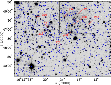
Figure 1: CamIV $H$-band image of the cluster [DBS2003] 157. The $\sim\!2\arcmin\times 2\arcmin$ black square surrounds the cluster as indicated in DBS2003. Blue marks denote all the sources found in the field by the daofind IRAF routine with a detection threshold of $4\sigma$ above the local background. The stars selected for the follow-up spectroscopy are numbered in red.

Figure 2: Top: Propagated photometric errors versus the $J$, $H$, and $K_{\rm s}$ magnitudes. Bottom: 2MASS versus CamIV magnitudes.

Standard procedures for NIR stellar CCD photometry in relatively crowded fields were performed with the IRAF software. All frames were individually dark-subtracted and flattened, and the background contribution subtracted. Eventually, they were aligned and trimmed, to finally generate J-, H- and K-band images by median-combining all frames of each filter. By choosing the median-filter, we diminished the influence of bad pixels and cosmic rays on the final image. This procedure resulted in $J$, $H$, and $K_{\rm s}$ “final” frames centred at $\mathrm{RA}({\rm J2000})=16^{\mathrm{h}}12^{\mathrm{m}}24^{\mathrm{s}}$, $\mathrm{Dec.}({\rm J2000})=-51\degr 47\arcmin 27\arcsec$, covering an area in the sky of $\sim\!5\arcmin\times 4\arcmin$. Figure 1 shows one of these frames ($H$-band). The daofind IRAF routine was used in the determination of the physical coordinates of the stars in each frame, adopting an object detection threshold (in counts) of $4\sigma$ above the local background.

The instrumental magnitudes were computed using the daophot IRAF routines. Since some parts of the cluster are too crowded for aperture photometry, the point spread functions (PSFs) were obtained using the psf routine. Simultaneous PSF-fits for all the stars listed by daofind were performed with the allstar routine. A fitting radius of about $1\times\langle FWHM\rangle$ and a PSF radius of $\sim 3.5$ times this value was assumed for all stars.

The photometric calibration was performed using data from the 2MASS survey. For this task, seventy-three no-blended stars in both 2MASS and CamIV frames were chosen outside the $\sim\!2\arcmin\times 2\arcmin$ rectangular region (see Fig. 1) centred at the coordinates of [DBS2003] 157. Using the least squares method, we adjusted linear transformation equations for converting the instrumental magnitudes to the 2MASS system. The standard deviations of these transformations, defined as

$$\sigma^{2}=\frac{1}{n-2}\,\sum_{i}{\left[m_{\rm 2MASS}^{(i)}-\beta_{0}-\beta_{1}\,m_{\rm CamIV}^{(i)}\right]^{2}}\,,$$ (1)

were 0.034, 0.026, and 0.036 for the $J$, $H$, and $K_{\rm s}$ (C1) filters, respectively. The final photometric errors were obtained as the quadratic sum of the transformation errors and of the individual error in the instrumental magnitudes given by the allstar task. No significant $(J-H)$ and $(H-K)$ colour-dependence between 2MASS and CamIV photometric systems has been found (Roman-Lopes & Abraham, 2006b). Figure 2 shows the linear relation observed between the 2MASS and CamIV magnitudes and the dependence of the errors on the photometric magnitude for all stars detected. By analysing the magnitude histograms, $\log(N)$ vs. $m$, we estimate the completeness limits of the photometry as $J=15.5$ mag, $H=15.2$ mag, and $K_{\rm s}=13.5$ mag, defined as the point where the $\log(N)$ vs. $m$ plot deviates from a straight line. These values are similar to the 2MASS limits on the $J$ and $H$ bands ($15.8$ and $15.1$ mag, respectively), but the $K_{\rm s}$ completeness limit of the CamIV data is $0.8$ mag lower.

Table 5 presents the results of the photometry. Columns 1 lists our identification of the star; columns 2 and 3 provide the equatorial coordinates obtained with the ccmap IRAF routine applied to pixel-coordinates listed by the daofind; columns 4, 5 and 6 list the $J$, $H$, and $K_{\rm s}$ photometric magnitudes and errors.

At a spatial resolution twice as better as the 2MASS survey, we to identified many sources that were previously unresolved in the 2MASS data, which in turn improves significantly the photometric accuracy, especially for stars situated in the crowded areas.

2.2 Spectroscopy

NIR spectroscopic data of nine stars in the GAL 331.31-00.34 region were acquired with the Ohio State Infrared Imager/Spectrometer (OSIRIS) coupled to the 4.1-m telescope of the Southern Observatory for Astrophysical Research (SOAR), located at Cerro Pachon, Chilean Andes. Spectra in $J$-, $H$-, and $K_{\rm s}$-band were taken with OSIRIS in the low-resolution (R $\simeq$ 1200) multi-order cross-dispersed (XD) mode. In this mode, the instrument operates with a f/2.8 camera and a short (27″$\times$ 1″) slit, covering the three bands simultaneously, in adjacent orders. The raw spectra were acquired using the standard AB nodding technique. Multiple short exposures were taken at each nod position, totalling 8-to-20 individual frames, giving a “final” exposure time of 8-to-40 minutes. Table LABEL:List_of_spectroscopic_targets presents a journal of the spectroscopic observations. It lists our identification of the star, as defined in Table 5, the identification in the 2MASS catalogue, the number and the duration of the individual exposures, and the observation dates. All the target stars were OB candidates selected from our photometry, with one exception: IRS 339, observed in 2008 and selected from an initial analysis based on the 2MASS data.

Table 1: Journal of spectroscopic observations

ID		Indiv. exp.	No of	Date
This work	2MASS	time (s)	exp.
IRS 339	J16122002-5146262	120	16	2008/07/10
IRS 298	J16122053-5146460	75	12	2011/05/08
IRS 287	J16122911-5146503	75	12	2011/05/08
IRS 497	J16122925-5147004	120	12	2011/06/02
IRS 355	J16123324-5146173	100	08	2011/06/02
IRS 176	J16122445-5147492	120	12	2011/06/03
IRS 444	J16122071-5147075	90	08	2011/06/03
IRS 289	J16121561-5146504	75	20	2011/06/12
IRS 452	J16122326-5146188	120	20	2011/06/12

A- and G-type spectroscopic standard stars were observed immediately before and after the “science” targets at similar air masses in order to remove telluric atmospheric absorption effects from the “science” spectra. These raw spectra were reduced using the CIRRED package and usual IRAF tasks. Two-dimensional frames were sky-subtracted for each pair of images taken at the two nod positions A and B, followed by dividing of the resultant image by a master flat. Thereafter, wavelength calibration was applied using sky lines; the typical error (1 $\sigma$) for this calibration is estimate as $\sim$12 Å. The multiple exposures were combined and one-dimensional spectra were generated.

Telluric atmospheric correction using the spectroscopic standard stars completed the reduction process. In this last step, we divided each “science” spectrum by the spectrum of the A0 V spectroscopic standard star free of photospheric features, carefully removed by interpolating across their wings using the continuum points on both sides of the line. In the case of the $H$-band, the subtraction of the hydrogen absorption lines could not be successfully done by this method because of the small separation between the multiple lines of the Brackett series and some strong telluric features. Therefore we proceeded to remove the hydrogen lines from the A0 V $H$-band spectrum using the technique used by Blum et al. (1997). Basically, one obtains a spectrum composed of only the profiles of hydrogen lines dividing the spectrum of a A-type standard star by a spectrum of a G-type star, whose H i intrinsic lines (fairly weaker than in A0 V line spectra) and other features of G-type spectra were previously removed by hand, using as template the NOAO solar atlas of Livingston & Wallace (1991). After that, these profiles are used to correct the A0 V spectrum, generating an $H$-band spectrum free of the hydrogen Brackett lines. Finally, telluric bands were removed using the IRAF task telluric. This algorithm interactively minimizes the RMS in specific regions of the sample by adjusting the wavelength shifts and intensity scales between the standard and “science” spectrum before performing the division. The wavelenght shifting corrects possible errors in the dispersion zero-points, whereas the intensity scaling equalizes airmass differences and variations in the abundance of the telluric species. Typical values of the shifts varied around $\sim$2 Å, while the scaling factors were smaller than 10%.

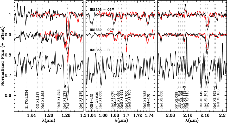
Figure 3: Spectra of the hot stars identified in the field of GAL 331.31-00.34 (in black) and the comparison spectra for a O6 V star (HD 101190) and a O9 V star (HD 93028) (in red).

3 Results

3.1 Spectral classification

He i optical absorption lines are well-known spectral features of OB stars (cf. Walborn & Fitzpatrick, 1990). If He ii absorption lines are also present, there is a substantial indicative of an O-type star. Since such features are also found in NIR spectra (Hanson et al., 1996), the presence of these lines must still be the primary criterion to be observed when classifying hot star spectra in this band. H i Brackett series could also be used. However, it would require special attention since these lines are highly contaminated by nebular emission (Bik et al., 2005).

Figure 4: Equivalent width $W_{\lambda}$ of He-lines versus the spectral type of dwarf stars (filled symbols) and a comparison with the values of $W_{\lambda}$ measured for IRS 298 and IRS 339 (open symbols, plotted at the spectral types O6 and O9, respectively).

The spectra of six of the stars listed in Table LABEL:List_of_spectroscopic_targets were found to correspond to late-type objects. They were classified visually by comparison with the 0.8-5 $\micron$ spectral library of cool stars by Rayner et al. (2009) and are displayed in Fig. 11 (Appendix). They are probably field stars and will not be included in our discussion on the region. The other three spectra correspond to early-type stars (Figure 3).

The detection of He ii lines at 1.692 $\mu$m and 2.188 $\mu$m in the spectra of IRS 298 and IRS 339 restricts the spectral types of both of these stars to O9 or earlier. On the other hand, the relative strength of these lines compared with the He i features at 1.279 $\mu$m, 1.700 $\mu$m and 2.112 $\mu$m indicates that IRS 339 is a late-O, whereas IRS 298 is an early-O star. The detection of the N iii line at 2.115 $\mu$m in emission, together with the broad profile of the H i lines, indicates that these two objects are dwarf stars, even though we do not discard that IRS 339 may be a supergiant. The distinction between the various luminosity classes can be doubtful in the NIR because of the paucity of lines suitable for this purpose and the large uncertainties of their equivalent widths (Hanson et al., 1996, 2005).

Figure 4 presents a comparison between the equivalent widths ($W_{\lambda}$) of four selected He lines of dwarf stars, ranging from O6 to O9.5 spectral types, along with the values measured for IRS 339 and IRS 298. In this comparison, we included only lines with equivalent widths reasonably well determined and discarded H i lines, whose profiles are highly dependent on the reduction process (see Sec. 2.2). Based on this scheme, the arguments presented above, and a visual comparison with other dwarf O-star spectra obtained with the same instrumental configuration and the spectra of the atlases by Hanson et al. (1996, 2005) and Bik et al. (2005), we classified IRS 298 as O6 V and IRS 339 as O9 V.

The third stellar spectrum displayed in Fig. 3 is too noisy to be accurately classified. However, the strength of its He i lines and the tentative detection of Si, C, N, O suggest that IRS 335 is an O9-to-B1 type star.

3.2 Spectroscopic parallax distance

The distances of the classified stars IRS 298 and IRS 339 have been calculated from their apparent $J$ and $H$ magnitudes listed in Table 5 using the method of spectroscopic parallax. The IR extinction curve by Stead & Hoare (2009), which results in $E_{J-H}/E_{H-K}=1.91$, was adopted for the reddening corrections. As intrinsic stellar parameters, we used the absolute magnitudes for the various spectral types compilated by Vacca et al. (1996) and the non-reddened colour indices by Koornneef (1983), both transformed into the 2MASS photometric system using the relations given by Carpenter (2001). According to this method, we obtained a heliocentric distance of $d=3.24\pm 0.56$ kpc ($A_{J}=3.03,A_{V}=10.44$) for IRS 339 and $d=3.35\pm 0.61$ kpc for IRS 298 ($A_{J}=3.51,A_{V}=12.10$). Based on the average distance of these two stars, we estimate the heliocentric distance for the H ii region GAL 331.31-00.34 of $d=3.29\pm 0.58$ kpc and a visual extinction of $\langle A_{V}\rangle\sim 11$ mag.

Caswell & Haynes (1987) obtained the radial velocity of $V_{\mathrm{LSR}}=-64$ km s^-1 for GAL 331.31-00.34, based on radio recombination lines. According to the model of Brand & Blitz (1993) for the rotation curve of the Galaxy, this figure corresponds to the near and far kinematic distances of $4.2$ kpc and $10.7$ kpc, respectively. Thus this Hii region is definitely at the near kinematic distance.

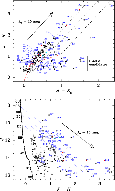
Figure 5: Top: $JHK$ colour-colour diagram. The solid red line depicts the main and the giant sequences (only from G3III-type on), the dashed red line represents a classical T-Tauri star, and the dotted, dashed, and dot-dashed black lines show the reddening lines for M-type, O-type dwarf stars, and classical T-Tauri, respectively (References in section 3.3). Bottom: colour-magnitude diagram. The black line represents the main sequence for the distance of 3.29 kpc. In both diagrams, the filled circles refer to the stars in the black square shown in Fig. 1, whereas the open circles refer to the other stars on the frame. The spectroscopically classified stars are indicated by blue (early-type) or red circles (late-type). Reddening lines for the 5 potential ionizing stars are also indicated.

3.3 Inventory of the ionizing stars and the Lyman continuum luminosity

In order to search other potential ionizing stars besides those confirmed spectroscopically, we reanalysed the NIR colour-colour (CC) and colour-magnitude (CM) diagrams (Figs. 5), assuming the distance of 3.29 kpc obtained in section 3.2. The intrinsic colours assumed are given by Koornneef (1983), while the absolute magnitudes in $J$-band are from Vacca et al. (1996) for O-stars and from Wegner (2007) for the other spectral types, all of them transformed into the 2MASS photometric system by the relations given by Carpenter (2001). The classical T-Tauri star locus shown in the CC diagram is taken from Meyer et al. (1997), while the locus of the Herbig Ae/Be candidates is indicated in accordance with Lada & Adams (1992). According to the CC diagram, we suspect that IRS 114 and IRS 446 are stars with spectral types between B0 V and B1 V. However, they are heavily obscured by dust ($A_{V}>18$ mag) and, in this region of the diagram, the classification is highly dependent on the slope adopted for the reddening vector. Nishiyama et al. (2006) and Stead & Hoare (2009) showed that this slope depends on the direction of observation and, for large reddening, the scattering around the reddening vector might be very high. In these cases, a purely-photometric classification may not be very accurate. Thus, it could not be discarded that IRS 114 and IRS 446 actually are pre-main sequence stars.

An inventory of our search for hot stars in the field is presented in Table 2, which lists the five stars identified as potential ionizing sources of GAL 331.31-00.34 along with their photometric and spectroscopic spectral classifications.

Table 2: Ionizing stars identified in GAL 331.31-00.34

Star ID			Classifications
This work	2MASS		Photometrical	Spectral
IRS 298	J16122053-5146460		mid-O	O6 V
IRS 339	J16122002-5146262		late-O	O9 V
IRS 355	J16123324-5146173		B0:	B0:
IRS 114	J16123539-5148304		B1:	$\cdots$
IRS 446	J16120863-5146482		B0:	$\cdots$

To test the completeness of the set of ionizing stars found associated with this Hii region, we compare the Lyman continuum photon luminosity $N_{\rm Ly}$ (photon s^-1) emitted by these stars with that needed to supply the radio continuum flux. Adopting the Lyman luminosity by Hanson et al. (1997), these five stars would amount to a total of $N_{\rm Ly}=10^{49.07}$ photons s^-1. In fact, this total is strongly dominated by the contribution of the two O-type stars. On the other hand, a Lyman continuum luminosity of $N_{\rm Ly}=10^{48.74}$ photons s^-1 is inferred from the radio continuum flux density $S_{\!\nu}$ at $22$ GHz measured by Amaral & Abraham (1991), using the expression: (see Rubin, 1968)

$$N_{\rm Ly}=\frac{5.59\times 10^{48}}{1+f_{i}\langle{\rm He^{+}/(H^{+}+He^{+})}\rangle}\left(\frac{\nu}{5\,{\rm GHz}}\right)^{0.1}T_{\mathrm{e}}^{-0.45}S_{\!\nu}d^{2},$$ (2)

where we assume the abundance ratio of ${\rm He}^{+}/{\rm H}^{+}=0.5$, a typical electron temperature $T_{\mathrm{e}}=8000$ K, and $f_{i}=0.65$ for the fraction of He-recombination photons energetic enough to ionize the H. Using the flux densities at 5 GHz measured by Caswell & Haynes (1987) and Kuchar & Clark (1997) almost identical results are found. Thus, we conclude that the O-type stars IRS 298 and IRS 339 can cope with the ionization of this nebula. The three stars photometrically classified as B0-to-B1 V type and other cooler stars would not contribute significantly to the ionization of the nebula.

3.4 YSO candidates

The intrinsic IR excess found in some stellar objects is an evidence of accreting disks or infalling envelopes. The identification of a group of objects with these properties indicates the existence of intense and recent star formation, which makes these regions interesting places to search for pre-main-sequence stellar objects (PMS), for example. The analysis of NIR and MIR colour-colour diagrams allows us to identify PMS stars and infer their nature based on their photometric properties. For example, according to Allen et al. (2004), objects with accreting disks, named Class II YSO, occupy the locus of reddened classical T-Tauri in NIR colour-colour diagrams, whereas objects whose emission is dominated by infalling envelopes, named Class I, have more reddened colours. YSOs with weak or no IR-excess are named Class III, and are not discriminated in CC diagrams, since they are found along with ZAMS stars.

Figure 6: MIR colour-colour diagram of stars in a region with $2\aas@@fstack{\prime}5$ of radius and centre matching with $H$-band frame presented in Fig. 1. YSOs with MIR colour excesses lie rightward of the dotted line. Class III YSOs and back/foreground objects must fall in the clump around the $(0,0)$ point.

Table 3: Young Stellar Objects candidates from the NIR photometry

Identifier			Class.
This work	2MASS	GLIMPSE
IRS 42	J16123385-5149269	G331.3195-00.3979	H AeBe
IRS 94	J16122500-5148459	$\cdots$	H AeBe
IRS 114	J16123539-5148304	G331.3330-00.3892	T Tau†
IRS 133	J16121385-5148204	G331.2944-00.3491	H AeBe
IRS 138	J16122037-5148157	G331.3076-00.3597	H AeBe
IRS 150	J16123309-5148076	G331.3331-00.3806	T Tau
IRS 172	J16120964-5147550	$\cdots$	T Tau
IRS 178	J16123437-5147487	G331.3391-00.3790	H AeBe
IRS 184	J16121891-5147434	G331.3110-00.3506	H AeBe
IRS 197	J16121395-5147382	G331.3025-00.3409	H AeBe
IRS 224	J16121561-5147255	$\cdots$	H AeBe
IRS 246	J16121386-5147139	G331.3071-00.3357	H AeBe
IRS 256	J16122966-5147088	$\cdots$	H AeBe
IRS 283	J16123053-5146525	$\cdots$	H AeBe
IRS 330	J16122692-5146314	$\cdots$	H AeBe
IRS 337	$\cdots$	$\cdots$	H AeBe
IRS 344	J16122121-5146255	$\cdots$	H AeBe
IRS 362	J16122064-5146136	$\cdots$	H AeBe
IRS 376	J16121207-5146026	$\cdots$	H AeBe
IRS 383	J16121868-5145597	$\cdots$	H AeBe
IRS 390	J16123848-5145538	G331.3687-00.3630	T Tau
IRS 402	J16123964-5145474	$\cdots$	H AeBe
IRS 445	J16122483-5146507	$\cdots$	H AeBe
IRS 446	J16120863-5146482	G331.3022-00.3213	T Tau†
IRS 454	J16122704-5146168	G331.3427-00.3474	T Tau
IRS 478	J16122996-5148154	G331.3258-00.3766	H AeBe
IRS 481	J16122752-5148042	G331.3232-00.3700	T Tau
IRS 483	J16121153-5147565	G331.2947-00.3402	H AeBe
IRS 484	J16122607-5147546	G331.3223-00.3655	H AeBe
IRS 487	J16122611-5147500	G331.3232-00.3646	T Tau
IRS 488	J16120772-5147483	G331.2891-00.3319	H AeBe
IRS 510	J16122112-5146395	G331.3274-00.3416	T Tau
IRS 511	J16120732-5146382	$\cdots$	H AeBe
IRS 524	J16123883-5148207	G331.3413-00.3932	H AeBe
IRS 531	J16120752-5146336	G331.3028-00.3164	H AeBe
IRS 533	$\cdots$	$\cdots$	H AeBe
$\dagger$See Section 3.3.

Table 4: Identifiers of the YSOs candidates from the MIR GLIMPSE photometry

This work			Surveys
MIR	NIR		GLIMPSE	2MASS
CE 1	$\cdots$		G331.2999-00.3784	J16122314-5149240
CE 2	$\cdots$		G331.3093-00.3762	J16122521-5148551
CE 3	$\cdots$		G331.3205-00.3817	$\cdots$
CE 4	IRS 552		G331.3131-00.3653	J16122341-5148167
CE 5	IRS 168		G331.3298-00.3735	J16123029-5147575
CE 6	IRS 176		G331.3203-00.3615	J16122445-5147492
CE 7	$\cdots$		G331.3341-00.3619	J16122844-5147163
CE 8	IRS 645		G331.3541-00.3664	J16123527-5146387
CE 9	IRS 355		G331.3543-00.3585	J16123324-5146173
CE 10	$\cdots$		G331.3416-00.3464	J16122648-5146177
CE 11	$\cdots$		G331.3497-00.3497	$\cdots$

Figure 7: Spectral energy distributions (between 1.25 and 10 $\mu$m) of objects with MIR colour excess. Photometric data extracted from the 2MASS and GLIMPSE surveys.

Figure 8: Spectral energy distribution (between 1.25 and 100 $\mu$m) of the source CE 10 based on data extracted from the 2MASS, GLIMPSE, and IRAS surveys. The dotted line (with spectral index of $\alpha\approx 3.6$) represents the fitting of the SED between $2$ and $25\,\mu$m.

The analysis of the NIR colour-colour diagram presented in Fig. 5 indicates a total of 36 YSO candidates, which are listed in Table 3 together with their tentative classification between T-Tauri (T Tau) or Herbig Ae/Be (H AeBe) stars. In this list, IRS 446 and IRS 114 could also be main sequence stars very obscured by dust. IRS 150 is the most reddened object detected in this work, with $A_{V}\ga 20$ mag. Considering the error bars of the photometry and extinction laws, IRS 150 has colours of a very reddened T-Tauri star. Redwards in the CC NIR diagram, IRS 478 presents typical colours of a very embedded YSO in an early stage of formation. A third group of stars appears below the T-Tauri locus, showing $(H-K_{s})\ga 0.4$ mag. In this region, Herbig Ae/Be stars, which are PMS stars more massive than T-Tauri, can be confused with Class I sources (Lada & Adams, 1992), galaxies or other background objects, making a classification based only on photometric data unreliable.

Figure 6 presents a MIR colour-colour diagram made with data from the GLIMPSE survey. This diagram is used to identify and classify objects with MIR colour excess (hereafter denoted as CE). Within a region of $2\aas@@fstack{\prime}5$ radius centred at the NIR $H$-frame (see Fig. 1), a total of 58 sources were simultaneously detected in the four GLIMPSE/IRAC-bands. We identify 11 MIR sources with colour excesses, which are listed in Table LABEL:MidIR_YSOs. Some of them are so obscured by dust that they have not been detected in the NIR bands.

Low-mass objects with MIR colour excess can be classified according to scheme by Allen et al. (2004). Class III objects, along with back/foreground objects, have the MIR colours $[3.6]-[4.5]\approx 0$ and $[5.8]-[8.0]\approx 0$, Class II have colours within $0\la[3.6]-[4.5]\la 0.8$ and $0.4\la[5.8]-[8.0]\la 1.1$, whereas Class I objects are expected to present colours $[3.6]-[4.5]\ga 0.7$ and $[5.8]-[8.0]\ga 1.0$. However, from the MIR photometry alone, we are not able to decide whether or not these objects are low-mass YSOs.

Figure 7 presents the spectral energy distributions (SEDs) of the MIR sources classified as YSOs, obtained by combining their NIR and MIR magnitudes. Sources CE 1 and CE 10 present a high spectral index $\alpha\equiv d\log{(\lambda F_{\lambda})}/d\log{\lambda}$ near $\lambda\sim 2\,\mu$m, which is characteristic of protostars in an early stage of evolution (Lada, 1987).

3.5 The nature of IRAS 16085-5138

IRAS 16085-5138 is the only IRAS source in the field. According to the classification scheme of Wood & Churchwell (1989), its IRAS colours are compatible with an ultra-compact H ii region. Methanol and hydroxyl masers have been detected at its vicinity (e.g. Caswell et al., 1980, 2000). We identify this source with CE 10, which presents the highest spectral index among all the CE-objects identified in this work, and is the only one detected inside the IRAS position error ellipse. Using photometric data from the 2MASS, GLIMPSE, and IRAS surveys, we obtained the 2–100 $\mu$m SED of this source (Fig. 8). According to Lada (1987), a spectral energy distribution rising longward of $\lambda=2\,\mu$m, such as that shown by this object, is characteristic of Class I objects. We evaluated the spectral index between $2$ and $25\,\mu$m (the dotted line in Fig. 8), and found $\alpha\approx 3.6$, typical of YSO immersed in a dense protostellar envelope, which is also in accordance with the classification drawn from the MIR colour-colour diagram.

Since most of the energy of this object is emitted in the infrared, the bolometric luminosity of the embedded protostar can be approximated by integrating the SED between $2$ and $100\,\mu$m. Adopting the distance of 3.29 kpc and $A_{V}=10$ mag, we obtain a luminosity of $L=7.7\times 10^{3}L_{\sun}$. Since pre-main-sequence models (e.g. Iben, 1965) indicate that early-type stars evolve at constant luminosity from the Hayashi track up to the main sequence, this result implies that the lower limit for this stellar mass is $M\ga 10\,M_{\sun}$. This mass value corresponds to a B0–B1 ZAMS star (cf. Hanson et al., 1997).

3.6 MIR shell structure

Figure 9 presents a RGB combination of $8.0\,\mu$m (R), $5.8\,\mu$m (G), and $3.6\,\mu$m (B) GLIMPSE images that show a broken shell-like structure with a diameter of $\approx\!4\arcmin$ associated with GAL 331.31-00.34. At the distance of 3.29 kpc, this shell would have a diameter of $\approx\!3.8$ parsec. This shell, identified as [CPA2006] S62 in the SIMBAD database, is named S 62 in the catalogue by Churchwell et al. (2006), which contains over 300 MIR arcs. The authors interpreted the arcs as the projection on the sky of three-dimensional bubbles, and found that only one quarter of them would be associated with H ii regions. In these cases, the bubbles would be expanding driven by the stellar wind and the radiation pressure from young massive stars. These stars would also power the bubbles, which are traced by the polycyclic aromatic hydrocarbon (PAH) emission produced in the photodissociation regions located at the edge of the H ii regions. According to Deharveng et al. (2010), most of the bubbles are in fact associated with H ii regions, and more than a quarter of them could be triggering the formation of a new generation of stars, as seems to be the case of RCW 120 (Deharveng et al., 2009).

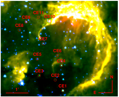
Figure 9: RGB combination of $8.0\,\mu$m (R), $5.8\,\mu$m (G), and $3.6\,\mu$m (B) GLIMPSE images. The red circles indicate the objects showing MIR colour excess listed in Table LABEL:MidIR_YSOs. In these three MIR bands, the peak emission coincides with the source CE 10, which we identified as the GLIMPSE counterpart of IRAS 16085-5138.

In the case of GAL 331.31-00.34, the IRAS source 16085-5138 and the methanol and hydroxyl masers (Ellingsen et al., 1996; Kuchar & Clark, 1997; Walsh et al., 1998; Caswell et al., 2000, 1980), typical tracers of ongoing massive star formation, are located at the bright northern border of the shell. At these positions, CS(2-1) and SiO molecular emission, which require densities higher than $10^{4}$ cm^-3, were detected by Bronfman et al. (1996) and Harju et al. (1998), respectively, who carried out radio surveys towards IRAS sources with colours of UC-HII regions. This possibly indicates that the expansion of the northern part of the bubble has been hampered by a dense molecular environment. The same phenomenon may also occur in other parts of the bubble, but additional observations of CS and NH₃, which are good tracers of dense molecular regions, are still lacking.

We also find that the T Tauri and the Herbig Ae/Be candidates found from the NIR photometry are found preferentially towards the bubble, while the YSO candidates found from the MIR data are located in a limited north-south band crossing the openings of the broken shell.

4 Summary

We carried out $JHK$ photometry in the direction of the Galactic H ii region GAL 331.31-00.34. We classified spectroscopically the main ionizing sources and estimated their distance. As a result, we identified other potential ionizing stars and performed their respective photometric classifications. Data from the 2MASS, GLIMPSE, and IRAS surveys were also explored. Our main findings are:

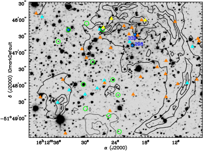
Figure 10: Contour levels of the IRAC $8.0\,\mu$m image superimposed on $H$-band image. The yellow triangles show the positions of the methanol and hydroxyl maser sources. The cyan and orange triangles locate the low-mass and high-mass YSO candidates (possible reddened T-Tauri and the Herbig Ae/Be stars, respectively) classified according to the NIR photometry and listed in Table 3. The green circles indicate the objects showing MIR colour excess listed in Table LABEL:MidIR_YSOs. The blue dots point to the hot stars spectroscopically identified.

1. We identified, classified spectroscopically, and estimated the spectroscopic parallax distances of two O-type stars associated with this Hii region: IRS 298 (O6 V, $d=3.35\pm 0.61$ kpc) and IRS 339 (O9 V, $d=3.24\pm 0.56$ kpc). Adopting the average distance of $3.29\pm 0.58$ kpc and comparing the Lyman continuum luminosity of these stars with that required to ionize the nebula, obtained from radio continuum observations, we concluded that these two stars are the ionizing sources of GAL 331.31-00.34.

2. By analysing the NIR colour-colour diagram, 36 pre-main sequence (PMS) objects could be identified and classified: 9 T-Tauri and 27 Herbig Ae/Be candidates. From the GLIMPSE data, 11 objects with MIR colour excesses have been found.

3. The MIR counterpart of the IRAS source 16085-5138 was identified and its spectral energy distribution between $2$ and $100\,\mu$m was analysed. We concluded that IRAS 16085-5138 is a massive YSO in an early stage of formation, with luminosity $L\geq 7.7\times 10^{3}L_{\sun}$ and mass $M>10\,M_{\sun}$.

High spatial resolution observations in radio frequency of the ionized and molecular gas are necessary for deeper studies of the dynamics and evolution of star formation in the field of GAL 331.31-00.34. Likewise, the possible connection between the diffuse high energy gamma-ray emission HESS J1614-518 and powerful winds and radiation fields of OB stars in the region should be subject of future hydrodynamic studies.

Appendix A

Figure 11: Cold stars in the field of GAL 331.31-00.34.

Table 5: $JHK$ photometry

IRS	$\alpha$(J2000)	$\delta$(J2000)	$J$	$H$	$K_{\rm s}$
3	16:12:33.028	-51:49:23.11	16.166$\pm$0.070	13.485$\pm$0.018	12.246$\pm$0.066
41	16:12:26.166	-51:49:27.27	13.479$\pm$0.028	11.951$\pm$0.016	11.199$\pm$0.037
42	16:12:33.848	-51:49:26.83	13.792$\pm$0.031	13.405$\pm$0.014	13.046$\pm$0.112
79	16:12:14.127	-51:49:03.79	11.658$\pm$0.029	9.809 $\pm$0.015	9.021 $\pm$0.015
87	16:12:37.336	-51:48:57.01	13.042$\pm$0.025	11.841$\pm$0.012	11.447$\pm$0.039
94	16:12:24.999	-51:48:45.83	14.965$\pm$0.031	14.212$\pm$0.014	13.090$\pm$0.231
98	16:12:39.840	-51:48:41.18	9.475 $\pm$0.032	8.185 $\pm$0.013	7.682 $\pm$0.014
102	16:12:23.151	-51:48:40.40	9.738 $\pm$0.028	9.044 $\pm$0.008	8.824 $\pm$0.015
108	16:12:34.752	-51:48:33.93	15.580$\pm$0.039	13.894$\pm$0.017	12.969$\pm$0.085
113	16:12:31.255	-51:48:30.62	12.930$\pm$0.028	11.270$\pm$0.009	10.601$\pm$0.018
114	16:12:35.383	-51:48:30.43	15.455$\pm$0.038	13.179$\pm$0.018	11.801$\pm$0.046
117	16:12:28.621	-51:48:29.84	12.435$\pm$0.029	11.468$\pm$0.014	11.163$\pm$0.022
133	16:12:13.855	-51:48:20.25	14.057$\pm$0.028	13.593$\pm$0.022	13.071$\pm$0.112
135	16:12:38.748	-51:48:16.20	10.923$\pm$0.029	10.217$\pm$0.013	9.954 $\pm$0.014
138	16:12:20.382	-51:48:15.79	14.586$\pm$0.025	14.140$\pm$0.024	13.745$\pm$0.196
150	16:12:33.097	-51:48:07.67	15.624$\pm$0.063	12.155$\pm$0.015	9.842 $\pm$0.013
164	16:12:13.044	-51:47:59.20	13.887$\pm$0.029	12.279$\pm$0.016	11.643$\pm$0.028
168	16:12:30.291	-51:47:57.57	11.302$\pm$0.026	10.720$\pm$0.015	10.448$\pm$0.013
169	16:12:31.902	-51:47:57.47	10.657$\pm$0.028	9.965 $\pm$0.013	9.775 $\pm$0.016
172	16:12:09.642	-51:47:54.88	15.896$\pm$0.060	14.828$\pm$0.042	13.973$\pm$0.360
176	16:12:24.451	-51:47:49.26	14.321$\pm$0.026	12.807$\pm$0.015	12.347$\pm$0.081
178	16:12:34.366	-51:47:48.61	13.576$\pm$0.029	13.295$\pm$0.010	12.752$\pm$0.131
184	16:12:18.908	-51:47:43.46	14.291$\pm$0.026	13.787$\pm$0.014	13.393$\pm$0.197
196	16:12:40.637	-51:47:37.13	11.914$\pm$0.032	10.663$\pm$0.012	10.148$\pm$0.015
197	16:12:13.960	-51:47:38.10	13.890$\pm$0.030	13.448$\pm$0.024	12.800$\pm$0.116
206	16:12:36.513	-51:47:32.56	12.382$\pm$0.027	11.490$\pm$0.016	11.162$\pm$0.021
217	16:12:19.360	-51:47:28.72	9.105 $\pm$0.025	8.155 $\pm$0.011	7.927 $\pm$0.014
224	16:12:15.607	-51:47:25.57	15.415$\pm$0.037	14.917$\pm$0.029	13.909$\pm$0.273
230	16:12:29.728	-51:47:19.69	14.678$\pm$0.036	11.831$\pm$0.016	10.561$\pm$0.018
234	16:12:12.487	-51:47:18.36	11.570$\pm$0.023	10.803$\pm$0.006	10.559$\pm$0.023
241	16:12:36.660	-51:47:15.40	15.811$\pm$0.061	13.884$\pm$0.022	12.786$\pm$0.115
246	16:12:13.859	-51:47:14.03	15.552$\pm$0.033	14.650$\pm$0.016	13.643$\pm$0.275
255	16:12:11.494	-51:47:09.36	15.466$\pm$0.080	14.015$\pm$0.028	13.145$\pm$0.090
256	16:12:29.659	-51:47:08.77	15.042$\pm$0.057	14.215$\pm$0.043	12.710$\pm$0.094
258	16:12:37.134	-51:47:07.52	11.005$\pm$0.029	10.247$\pm$0.009	9.977 $\pm$0.019
262	16:12:32.924	-51:47:05.09	12.240$\pm$0.026	11.318$\pm$0.010	10.978$\pm$0.021
264	16:12:28.519	-51:47:04.38	11.391$\pm$0.026	11.089$\pm$0.012	11.095$\pm$0.025
268	16:12:30.324	-51:47:01.98	11.528$\pm$0.024	10.457$\pm$0.014	10.035$\pm$0.016
277	16:12:26.742	-51:46:57.38	11.536$\pm$0.026	11.224$\pm$0.016	11.200$\pm$0.031
278	16:12:34.600	-51:46:56.74	10.497$\pm$0.027	9.805 $\pm$0.013	9.514 $\pm$0.017
283	16:12:30.538	-51:46:52.68	16.162$\pm$0.085	15.411$\pm$0.050	14.346$\pm$0.311
285	16:12:27.736	-51:46:50.82	15.592$\pm$0.056	13.071$\pm$0.010	12.046$\pm$0.043
286	16:12:19.625	-51:46:51.10	15.052$\pm$0.025	12.684$\pm$0.015	11.686$\pm$0.041
287	16:12:29.116	-51:46:50.29	11.203$\pm$0.025	10.169$\pm$0.009	9.736 $\pm$0.012
289	16:12:15.621	-51:46:50.44	14.330$\pm$0.021	11.136$\pm$0.012	9.643 $\pm$0.013
295	16:12:32.209	-51:46:46.38	15.284$\pm$0.037	11.904$\pm$0.011	10.302$\pm$0.013
298	16:12:20.539	-51:46:46.07	11.674$\pm$0.024	10.288$\pm$0.008	9.593 $\pm$0.018
319	16:12:27.952	-51:46:35.74	10.950$\pm$0.024	9.707 $\pm$0.012	9.216 $\pm$0.013
323	16:12:40.287	-51:46:34.17	14.192$\pm$0.026	12.371$\pm$0.017	11.540$\pm$0.034
324	16:12:09.102	-51:46:35.02	11.319$\pm$0.024	10.520$\pm$0.009	10.206$\pm$0.013
330	16:12:26.925	-51:46:31.44	14.564$\pm$0.025	13.945$\pm$0.017	13.499$\pm$0.192
337	16:12:19.501	-51:46:27.59	14.966$\pm$0.078	14.479$\pm$0.083	13.684$\pm$0.216
339	16:12:20.031	-51:46:26.20	11.784$\pm$0.024	10.596$\pm$0.007	10.001$\pm$0.016
344	16:12:21.212	-51:46:25.36	15.906$\pm$0.059	15.476$\pm$0.065	14.138$\pm$0.355
355	16:12:33.242	-51:46:17.41	11.728$\pm$0.022	10.691$\pm$0.015	10.184$\pm$0.015
362	16:12:20.653	-51:46:13.75	14.693$\pm$0.033	14.312$\pm$0.023	13.494$\pm$0.192
363	16:12:32.580	-51:46:13.00	12.597$\pm$0.026	11.052$\pm$0.014	10.408$\pm$0.018
369	16:12:36.212	-51:46:08.58	11.911$\pm$0.029	10.730$\pm$0.013	10.264$\pm$0.018
374	16:12:37.823	-51:46:03.37	14.042$\pm$0.026	12.130$\pm$0.012	11.320$\pm$0.031
375	16:12:35.031	-51:46:02.14	11.553$\pm$0.022	10.814$\pm$0.014	10.576$\pm$0.016
376	16:12:12.069	-51:46:02.71	14.307$\pm$0.026	14.016$\pm$0.018	13.579$\pm$0.240
383	16:12:18.702	-51:45:59.64	15.204$\pm$0.042	14.690$\pm$0.032	14.178$\pm$0.361
390	16:12:38.478	-51:45:53.96	13.809$\pm$0.027	12.774$\pm$0.017	12.078$\pm$0.047
391	16:12:27.182	-51:45:53.34	13.145$\pm$0.023	11.842$\pm$0.014	11.218$\pm$0.027
402	16:12:39.647	-51:45:47.38	15.766$\pm$0.057	15.167$\pm$0.039	14.322$\pm$0.353
410	16:12:35.158	-51:45:44.50	15.733$\pm$0.046	12.333$\pm$0.009	10.799$\pm$0.022
415	16:12:32.059	-51:45:39.79	11.884$\pm$0.025	11.189$\pm$0.014	10.925$\pm$0.020
416	16:12:23.793	-51:45:40.10	11.733$\pm$0.023	11.057$\pm$0.012	10.795$\pm$0.023
425	16:12:10.706	-51:48:53.63	13.672$\pm$0.026	12.021$\pm$0.013	11.346$\pm$0.031
440	16:12:07.291	-51:47:22.36	12.806$\pm$0.019	11.696$\pm$0.008	11.330$\pm$0.017
444	16:12:20.717	-51:47:07.66	11.615$\pm$0.035	10.535$\pm$0.052	10.144$\pm$0.050
445	16:12:24.838	-51:46:50.62	14.336$\pm$0.032	13.563$\pm$0.053	12.820$\pm$0.143
446	16:12:08.634	-51:46:48.29	15.899$\pm$0.085	13.180$\pm$0.019	11.566$\pm$0.033
452	16:12:23.287	-51:46:18.82	14.254$\pm$0.045	11.793$\pm$0.016	10.657$\pm$0.017
454	16:12:27.046	-51:46:16.80	14.315$\pm$0.033	13.110$\pm$0.019	12.295$\pm$0.066
478	16:12:29.948	-51:48:15.55	15.810$\pm$0.100	13.961$\pm$0.075	12.172$\pm$0.056
481	16:12:27.537	-51:48:04.28	15.985$\pm$0.101	14.350$\pm$0.055	13.074$\pm$0.134
483	16:12:11.536	-51:47:56.37	13.732$\pm$0.024	13.260$\pm$0.014	12.797$\pm$0.098
484	16:12:26.066	-51:47:54.60	15.870$\pm$0.068	15.093$\pm$0.097	13.571$\pm$0.221
487	16:12:26.122	-51:47:50.07	15.091$\pm$0.033	13.783$\pm$0.022	12.938$\pm$0.117
488	16:12:07.740	-51:47:48.32	14.966$\pm$0.058	14.385$\pm$0.053	13.608$\pm$0.199
493	16:12:28.866	-51:47:21.05	16.241$\pm$0.162	14.295$\pm$0.154	13.235$\pm$0.137
494	16:12:12.964	-51:47:13.43	12.650$\pm$0.023	11.589$\pm$0.011	11.183$\pm$0.021
497	16:12:29.250	-51:47:00.40	13.407$\pm$0.047	11.917$\pm$0.043	11.351$\pm$0.052
510	16:12:21.101	-51:46:39.48	16.272$\pm$0.160	14.472$\pm$0.032	13.269$\pm$0.110
511	16:12:07.325	-51:46:38.31	15.433$\pm$0.053	14.657$\pm$0.054	13.508$\pm$0.143
515	16:12:19.293	-51:46:07.20	12.907$\pm$0.028	11.880$\pm$0.022	11.509$\pm$0.035
524	16:12:38.811	-51:48:20.72	13.964$\pm$0.139	13.450$\pm$0.127	12.917$\pm$0.109
530	16:12:27.472	-51:46:54.64	15.507$\pm$0.163	13.005$\pm$0.045	12.004$\pm$0.061
531	16:12:07.529	-51:46:33.57	14.011$\pm$0.018	13.496$\pm$0.019	13.037$\pm$0.135
533	16:12:22.212	-51:46:10.27	15.790$\pm$0.058	15.166$\pm$0.026	14.192$\pm$0.242

References

- Allen et al. (2004) Allen, L. E., et al., 2004, ApJS, 154, 363
- Aharonian et al. (2006) Aharonian, F., et al., 2006, ApJ, 636, 777
- Aharonian et al. (2007) Aharonian F., et al., 2007, A&A, 467, 1075
- Amaral & Abraham (1991) Amaral, L. H., Abraham, Z., 1991, A&A, 251, 259
- Benjamin et al. (2003) Benjamin R. A., et al., 2003, PASP, 115, 953
- Bik et al. (2005) Bik, A., Kaper, L., Hanson, M. M., Smits, M., 2005, A&A, 440, 121
- Blum et al. (1997) Blum, R. D., Ramond, T. M., Conti, P. S., Figer, D. F., Sellgren, K., 1997, AJ, 113, 1855
- Brand & Blitz (1993) Brand, J., Blitz, L., 1993, A&A, 275, 67
- Bronfman et al. (1996) Bronfman, L., Nyman, L. A., May, J., 1996, A&AS, 115, 81
- Carpenter (2001) Carpenter, J. M., 2001, AJ, 121, 2851
- Caswell et al. (1980) Caswell, J. L., Haynes, R. F., Goss, W. M., 1980, Australian Journal of Physics, 33, 639
- Caswell & Haynes (1987) Caswell, J. L., Haynes, R. F., 1987, A&A, 171, 261
- Caswell et al. (2000) Caswell, J. L., Yi, J., Booth, R. S., Cragg, D. M., 2000, MNRAS, 313, 599
- Chavarría et al. (2010) Chavarría, L., Mardones, D., Garay, G., Escala, A., Bronfman, L., Lizano, S., 2010, ApJ, 710, 583
- Churchwell et al. (2006) Churchwell E., et al., 2006, ApJ, 649, 759
- Deharveng et al. (2009) Deharveng L., Zavagno A., Schuller F., Caplan J., Pomarès M., De Breuck C., 2009, A&A, 496, 177
- Deharveng et al. (2010) Deharveng L., et al., 2010, A&A, 523, A6
- Dutra et al. (2003) Dutra, C. M., Bica, E., Soares, J., Barbuy, B., 2003, A&A, 400, 533
- Ellingsen et al. (1996) Ellingsen, S. P., von Bibra, M. L., McCulloch, P. M., Norris, R. P., Deshpande, A. A., Phillips, C. J., 1996, MNRAS, 280, 378
- Hanson et al. (1996) Hanson, M. M., Conti, P. S., Rieke, M. J., 1996, ApJS, 107, 281
- Hanson et al. (1997) Hanson, M. M., Howarth, I. D., Conti, P. S., 1997, ApJ, 489, 698
- Hanson et al. (2005) Hanson, M. M., Kudritzki, R. P., Kenworthy, M. A., Puls, J., Tokunaga, A. T., 2005, ApJS, 161, 154
- Harju et al. (1998) Harju, J., Lehtinen, K., Booth, R. S., Zinchenko, I., 1998, A&AS, 132, 211
- Iben (1965) Iben, I., Jr., 1965, ApJ, 142, 421
- Koornneef (1983) Koornneef, J., 1983, A&A, 128, 84
- Kuchar & Clark (1997) Kuchar, T. A., Clark, F. O., 1997, ApJ, 488, 224
- Lada (1987) Lada, C. J., 1987, Star Forming Regions, 115, 1
- Lada & Adams (1992) Lada, C. J., Adams, F. C., 1992, ApJ, 393, 278
- Livingston & Wallace (1991) Livingston W., Wallace L., 1991, An atlas of the solar spectrum in the infrared from 1850 to 9000 cm-1 (1.1 to 5.4 micrometer). NSO Technical Report, Tucson: National Solar Observatory, National Optical Astronomy Observatory, 1991
- Meyer et al. (1997) Meyer, M. R., Calvet, N., Hillenbrand, L. A., 1997, AJ, 114, 288
- Nishiyama et al. (2006) Nishiyama, S., Nagata, T., Kusakabe, N., et al., 2006, ApJ, 638, 839
- Parizot et al. (2004) Parizot, E., Marcowith, A., van der Swaluw, E., Bykov, A. M., Tatischeff, V., 2004, A&A, 424, 747
- Rayner et al. (2009) Rayner, J. T., Cushing, M. C., Vacca, W. D., 2009, ApJS, 185, 289
- Rodgers et al. (1960) Rodgers, A. W., Campbell, C. T., Whiteoak, J. B., 1960, MNRAS, 121, 103
- Roman-Lopes et al. (2003) Roman-Lopes, A., Abraham, Z., Lépine, J. R. D., 2003, AJ, 126, 1896
- Roman-Lopes & Abraham (2004) Roman-Lopes, A., Abraham, Z., 2004, AJ, 127, 2817
- Roman-Lopes & Abraham (2006a) Roman-Lopes, A., Abraham, Z., 2006, AJ, 131, 951
- Roman-Lopes & Abraham (2006b) Roman-Lopes, A., Abraham, Z., 2006, AJ, 131, 2223
- Rubin (1968) Rubin, R. H., 1968, ApJ, 154, 391
- Russeil et al. (2005) Russeil, D., Adami, C., Amram, P., Le Coarer, E., Georgelin, Y. M., Marcelin, M., Parker, Q., 2005, A&A, 429, 497
- Skinner et al. (2009) Skinner, S. L., Sokal, K. R., Megeath, S. T., Güdel, M., Audard, M., Flaherty, K. M., Meyer, M. R., Damineli, A., 2009, ApJ, 701, 710
- Stead & Hoare (2009) Stead, J. J., Hoare, M. G., 2009, MNRAS, 400, 731
- Vacca et al. (1996) Vacca, W. D., Garmany, C. D., Shull, J. M., 1996, ApJ, 460, 914
- Walborn & Fitzpatrick (1990) Walborn, N. R., Fitzpatrick, E. L., 1990, PASP, 102, 379
- Walsh et al. (1997) Walsh, A. J., Hyland, A. R., Robinson, G., Burton, M. G., 1997, MNRAS, 291, 261
- Walsh et al. (1998) Walsh, A. J., Burton, M. G., Hyland, A. R., Robinson, G., 1998, MNRAS, 301, 640
- Wegner (2007) Wegner, W., 2007, MNRAS, 374, 1549
- Wood & Churchwell (1989) Wood, D. O. S., Churchwell, E., 1989, ApJ, 340, 265