The topological system with a twisting edge band: position-dependent Hall resistance

Abstract

We study a $\nu=1$ topological system with one twisting edge-state band and one normal edge-state band. For the twisting edge-state band, Fermi energy goes through the band three times, thus, having three edge states on one side of the sample; while the normal edge band contributes only one edge state on the other side of the sample. In such a system, we show that it consists of both topologically protected and unprotected edge states, and as a consequence, its Hall resistance depends on the location where the Hall measurement is done even for a translationally invariant system. This unique property is absent in a normal topological insulator.

Introduction: The topological system has attracted much attention in recent years rv1 ; rv2 . About twenty years ago, by proposing the quantum anomalous Hall effect (QAHE) in graphene haldane , Haldane gave a simple two-band model to study a topological system. Recently, the topological insulator material is first predicted and then experimentally observed in some two-dimensional (2D) systems addref1 ; 2Dth ; 2Dex . The three-dimension topological materials are also discovered soon after 3D .

In research of the robustness of topological system, the analysis of edge states is to be an effective approach edgestates . The helical edge states for 2D topological systems are shown to have the topological protection of $Z_{2}$ hedge , and the scattering between them is prohibited without breaking time reversal symmetry. While with edge bands distortion, they may cross the Fermi surface more than one time, which may also give rise to some extra edge states rv1 . However, these extra edge states can not bring new topological phases, and are not protected by the topology fu2007 . They are thought easy to be affected and are treated as unimportant in the earlier studies.

In this Letter, we show a nontrivial effect from the topological unprotected edge states. While a system is with both the topological protected and unprotected edge states, the Hall conductance depends on the measurement location even for a translationally invariant system. This novel property survives at a finite disorder, however, it is absent in both topological trivial systems and normal topological systems. Thus, this unique property is the hallmark of a topological system with a twisting edge band.

Model and Hamiltonian: The band structure of our system is shown in Fig.1(A). Below we provide one example of how to achieve this band structure. Without loss of generality, we take the simple $\nu=1$ topological system as an example, which consists of one pair of topological protected edge states. The AB-stacked square lattice QAHE system liu2011 is chosen, in which the two type of atoms are needed. As shown in Fig. 1(C), we can assume atom $A$ at $s$ level and atom $B$ at the lowest $p$ level wu2010 . Generally, this $p$-orbital may not along the direction of lattice structure, here we choose it along $\pm\vec{e}_{1}$-direction. The check board magnetic field is also applied by the Peierls phase $\phi_{0}=\pi/2$ when an electron jumps from $A$ to $B$ along $\pm\vec{e}_{y}$-direction. Supposing the on-site energy of $A$ and $B$ are the same, set to be the zero energy point. The tight-binding Hamiltonian can thus be written as $H=H_{1}+H_{2}$, with $H_{1}$ ($H_{2}$) the nearest (next-nearest) hopping Hamiltonian:

$$H_{1} = -t_{ab}\sum_{\mathbf{i}}\left[b_{\mathbf{i}+\delta x}^{{\dagger}}a_{\mathbf{i}}+{\mathrm{e}}^{{\mathrm{i}}\phi_{0}}b_{\mathbf{i}+\delta y}^{{\dagger}}a_{\mathbf{i}}+h.c.\right]$$ (1)

$$+t_{ab}\sum_{\mathbf{i}}\left[a_{\mathbf{i}+\delta x}^{{\dagger}}b_{\mathbf{i}}+{\mathrm{e}}^{-{\mathrm{i}}\phi_{0}}a_{\mathbf{i}+\delta y}^{{\dagger}}b_{\mathbf{i}}+h.c.\right]$$

$$H_{2} = -\sum_{\mathbf{i}}\left[t_{a1}a_{\mathbf{i}+\delta e1}^{{\dagger}}a_{\mathbf{i}}+t_{a2}a_{\mathbf{i}+\delta e2}^{{\dagger}}a_{\mathbf{i}}+h.c.\right]$$ (2)

$$-\sum_{\mathbf{i}}\left[t_{b1}b_{\mathbf{i}+\delta e1}^{{\dagger}}b_{\mathbf{i}}+t_{b2}b_{\mathbf{i}+\delta e2}^{{\dagger}}b_{\mathbf{i}}+h.c.\right]$$

Here $t_{ab}$ is the hopping term from $A$ to $B$ along the $+x$ and $+y$-directions, set to be positive; while the hopping from $B$ to $A$ along the same direction get a negative sign. $t_{a1}$ and $t_{a2}$ are the next nearest neighbor hopping at $A$ sublattice along $\vec{e}_{1}$ and $\vec{e}_{2}$, respectively. $t_{b1}$ and $t_{b2}$ are the counterparts for the $B$ sublattice. One can check $t_{a1},t_{a2},t_{b2}>0$ and $t_{b1}<0$ from Fig. 1(C). Besides, we also have $t_{a1}=t_{a2}$ and $|t_{b1}|\neq|t_{b2}|$, due to the anisotropy of the $p$ level.

It is easy to discuss this tight-binding Hamiltonian in $\mathbf{k}$-space. Because the system is translationally invariant, we have $\mathcal{H}(\mathbf{k})=h_{0}(\mathbf{k})+\mathbf{\sigma}\cdot\mathbf{p}(\mathbf{k})$. Here $p_{x}(\mathbf{k})=2t_{ab}\sin(k_{y}a_{0})$, $p_{y}(\mathbf{k})=-2t_{ab}\sin(k_{x}a_{0})$. The next nearest hopping gives $p_{z}(\mathbf{k})=-[(t_{a1}-t_{b1})\cos(k_{x}a_{0}+k_{y}a_{0})+(t_{a2}-t_{b2})\cos(k_{x}a_{0}-k_{y}a_{0})]$ and a nonconstant $h_{0}(\mathbf{k})=-[(t_{a1}+t_{b1})\cos(k_{x}a_{0}+k_{y}a_{0})+(t_{a2}+t_{b2})\cos(k_{x}a_{0}-k_{y}a_{0})]$. Here $a_{0}$ is the distance between the nearest neighbor atoms $A$ and $B$. The Chern number of the system can be calculated in $\mathbf{k}$-space rv1 ; TKNN by $\nu=\int d^{2}\mathbf{k}\mathcal{F}/2\pi$. For our system, when there exists a real gap, the Chern number of the lower band gives $\nu=1$.

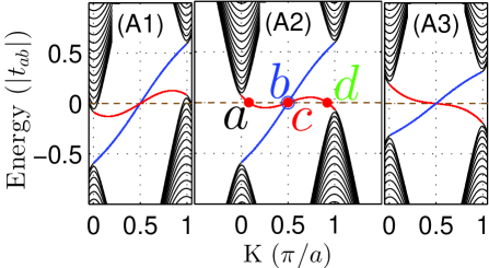
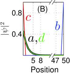
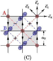
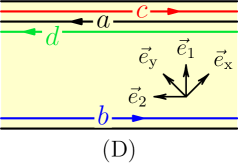
Figure 1: (Color online) (A) The energy band structures of zigzag-edge ribbon of topological system, with the ribbon width $W=50a$ and $a=\sqrt{2}a_{0}$. We choose the parameters $t_{ab}=10$ and $t_{a1}=t_{a2}=t_{c}+0.1$, $t_{b1}=-t_{c}-t_{s}$, $t_{b2}=t_{c}$ for all the subplots. (A1) indirect semi-metal with $t_{c}=1.4$ and $t_{s}=-0.4$, (A2) the twisting edge band system with $t_{c}=1.4$ and $t_{s}=0.4$, and (A3) the normal topological system with $t_{c}=0.7$ and $t_{s}=1$. (B) The distribution $|\psi|^{2}$ of the four edge states of (A2). (C) The lattice structure of the system. (D) The schematic diagram of the four edge states of (A2). (E) The twisting edge band of (A2) can be treated as mix of the topological protected and unprotected systems.

Twisting edge band: The coexistence of distorted edge band and normal edge band originates from the symmetry breaking of the eigenvalue $\lambda_{\pm}=h_{0}\pm|\mathbf{p}|$. These two eigenvalue correspond separately to the upper and down bands. Because of the next nearest hopping, the symmetry of $\lambda_{\pm}$ reduces from $C_{4}$ to $C_{2}$. The Dirac points at $(0,0)$ and $(\pm\pi,\pm\pi)$ have different energy values as the Dirac points at $(0,\pm\pi)$ and $(\pm\pi,0)$. If the system is constrained at $\vec{e}_{x}$ or $\vec{e}_{y}$ direction, each projected Dirac point in fact contains two type of Dirac points, so the projected Dirac points remains the same. However, if the system is constrained at $\vec{e}_{1}$-direction [see Fig.1(C)], i.e., if with the zigzag edge, each projected Dirac point contains only one type of Dirac point, the two projected Dirac points are different with each other, as shown in Fig.1(A). Consequently, the two edge bands may have different group velocities $|\partial\varepsilon(\mathbf{k})/\partial\mathbf{k}|$. In this way, the edge bands are distorted.

To get a twisting edge band, we need a little more effort. Define $A_{t}=(t_{a1}+t_{a2})$ and $B_{t}=(t_{b1}+t_{b2})$, we can get the bulk gap of the system as $\Delta=2(|A_{t}-B_{t}|-|A_{t}+B_{t}|)$. While $A_{t}B_{t}>0$ gives an indirect negative gap $\Delta$. In this case, although the system has a twisting edge band [see red curve in Fig.1(A1)], but it is without a bulk gap, which creates an indirect semi-metal. The bulk insulator needs $\Delta>0$ thus $A_{t}B_{t}<0$. When gap $\Delta$ is large, the system may only have a distorted edge band but no twisting edge band [see Fig.1(A3)], which is the normal 2D topological insulator. When gap $\Delta$ is positive but small, we may have a twisting edge band [Fig.1(A2)]. We also have another bigger ‘gap’ $\Delta_{2}=2(|A_{t}-B_{t}|+|A_{t}+B_{t}|)$, corresponding to the normal edge band [see the blue curve in Fig.1(A)]. In our system $A_{t}>0$, and it’s no harm to set $A_{t}>|B_{t}|$, then we can get $\Delta=-4B_{t}$ and $\Delta_{2}=4A_{t}$. This means that the twisting and normal edge bands are independently determined by $B_{t}$ and $A_{t}$, respectively. If we choose $t_{b1}=-t_{c}-t_{s}$, $t_{b2}=t_{c}$ with $t_{c},t_{s}>0$, the gap $\Delta$ is simplified to $\Delta=4t_{s}$.

Due to the edge band being twisted, it can cross Fermi surface $E_{F}$ three times, marked by $a$, $c$ and $d$ [see Fig.1(A2)]. The other normal edge band meets Fermi surface at $b$. Fig.1(B) shows the distribution $|\psi|^{2}$ v.s. location for these four states. We can see that, all four states are localized on the edges of the sample, the distribution is almost zero inside the bulk. Among them, the three states $a,c$ and $d$ are localized on the upper edge, while state $b$ is localized on the lower edge [see also Fig.1(D)]. As the Chern number of the system is $\nu=1$, only one pair of the edge states are protected by the topology, while another two are not protected. There is no doubt that $b$ is protected by topology since it is the only one edge state on the lower edge. The other topology protected state is a mixture of these three degenerated edge states $a,c$ and $d$ on the upper edge. Here we notice that the present system can be treated as the combination of the normal topological system plus a topological trivial system with one pair of unprotected edge states, as shown in Fig.1(E).

The translational invariance symmetry breaking of the Hall resistance. Now, let us study the transport property of the system using the $6$-lead set-up. As shown in Fig.2(c), lead-1 and lead-4 are made by the same materials of the sample, which can support the well-defined edge states inside the gap of sample. The vertical leads $2,3,5,6$ are made of a metal, which can afford as much modes as possible. A small longitudinal voltage gradient is applied by setting the lead-1 at $V/2$ and the lead-4 at $-V/2$, providing the longitudinal current $I_{1}$. We use the zero temperature Landauer-B$\ddot{u}$ttiker formula $I_{p}=\frac{e^{2}}{h}\sum_{q\neq p}(V_{p}-V_{q})T_{p,q}$, with $T_{p,q}$ the transmission coefficient from the lead $q$ to $p$ addref2 . The vertical voltage $V_{p}$ can thus be obtained by using the open boundary condition, i.e. by letting the corresponding leads to have zero current: $I_{p}=0$ with $p=2,3,5,6$. Finally, the Hall and longitudinal resistances can be obtained from $R_{p,q}\equiv(V_{p}-V_{q})/I_{1}$.

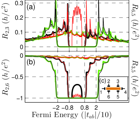
Figure 2: (Color online) For the three sets of parameters used in Fig.1(A), the corresponding resistances of the system v.s. the Fermi energy: (a) the longitudinal resistances and (b) the Hall resistances. The wide lines are for $R_{6,5}$ and $R_{2,6}$, the narrow lines are for $R_{2,3}$ and $R_{3,5}$. In both figures, the pair of lines with the broadest quantized plateau ($-2\sim 2$) are for Fig.1(A3); the pair of lines only have plateau within $-0.8\sim 0.8$ are for Fig.1(A2); for Fig.1(A1), the pair of lines have no plateau. Other parameters used for the calculation: the ribbon width $W=50a$, the distance between vertical leads $L=20a$. (c) is the schematic diagram of the $6$-lead measurement we used for (a) and (b).

For the three sets of parameters used in Fig.1(A), by changing the Fermi energy, in Fig.2(b) we plot the Hall resistance $R_{2,6}$, measured on the left side of the sample, and $R_{3,5}$, on the right side. We also draw in Fig.2(a) the longitudinal resistance $R_{2,3}$ for the upper edge, and $R_{6,5}$ for the bottom edge. For the parameters used in Fig.1(A1) with an indirect negative gap, the coexistence of twisting edge band and bulk band does not directly show a topological property. Two Hall (longitudinal) resistances are very small and almost equal, because that the system is translationally invariant. For the parameters used in Fig.1(A3), though the edge band is already somewhat distorted with two edge currents having different speeds, the measurement can give no new information other than the normal topological insulator. The Hall (longitudinal) resistances measured at different place (edge) are the same. Within the gap, the Hall resistances give a quantized plateau ($h/e^{2}$) characterized by the topological number $\nu=1$, and two longitudinal resistances are zero, because of the absence of back scattering.

For the parameters used in Fig.1(A2), the twisting edge band case, the results are very different and interesting. When the Fermi energy $E_{F}$ is within the gap but out of the range of the twisting of edge band, all measurements still show normal topological property by giving the plateau. When the Fermi energy goes within the twisting area, the situation is totally changed. Let us first look at the longitudinal resistance. We still have $R_{6,5}=0$, because there is only one edge state $b$ on the bottom edge of the sample, no back scattering is allowed there, the voltage drop is zero with $V_{6}=V_{5}$. However, on the upper edge, $R_{2,3}$ is nonzero and it is about $0.25h/e^{2}$. This is because we have three edge states on the upper edge, two of them move to the right and the other one moves to the left. As one pair of them moves in the opposite directions, not topologically protected, the back scattering is allowed. Thus, the voltage may drop, $V_{2}\neq V_{3}$ to give a nonzero resistance $R_{2,3}$ on the upper edge. Specifically, as lead-2 is on the left side of the lead-3, we have $V/2=V_{1}>V_{2}>V_{3}>V_{4}=-V/2$. The two Hall resistances also change and they are no longer equal to the value $h/\nu e^{2}$, although the Chern number of the system is still $\nu=1$. In particular, as $V_{2}\neq V_{3}$ and $V_{6}=V_{5}$, we can see that the left side Hall resistance $R_{2,6}=(V_{2}-V_{6})/I_{1}$ is no longer same as the right side Hall resistance $R_{3,5}=(V_{3}-V_{5})/I_{1}$: $|R_{2,6}|$ is decreased to about $0.7h/e^{2}$ within the twisting-edge-band region but $|R_{3,5}|$ is larger than $0.9h/e^{2}$. It should be emphasized again that the present system is translationally invariant. However, from the results above, the Hall resistance does break the translational invariance. This novel phenomenon, the breaking of the translational invariance of the Hall resistance in a translationally invariant system, origins from the twisting edge band and the combination of the topological protected and unprotected edge states. This property is unique to the topological system with a twisting edge band and can not be observed in either normal topological insulators or non-topological systems. In addition, we also witnessed the oscillation of $R_{3,5}$ and $R_{2,3}$ for the parameters used in Fig.1(A2). This is because of the Fabry-Perot interference between the lead-2 and lead-3. The number of oscillation are determined by the distance between them.

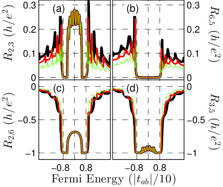
Figure 3: (Color online) For the parameters used in Fig.1(A2), the resistances v.s. Fermi energy for sample widthes $W=50a$ (the broadest black line), $60a$ (the red line), and $80a$ (the thinnest green line).

In order to confirm that the breaking of the translational invariance of Hall resistance is due to the edge states, we show the Hall and longitudinal resistances versus the width of the sample in Fig.3. The change of width only has the effect on the bulk bands and should not affect the edge bands when the sample is wide enough. From Fig.3, it can be seen that outside the gap, all the four resistances are changed when the width changes. However, within the gap, the resistances maintain the same for different widthes. It clearly shows that the breaking of the translational invariance of the Hall resistance does come from the twisting edge band.

One may argue that the 6-lead measurement itself already breaks the translational invariance, as the left Hall bar is close to the higher voltage side and the right Hall bar is close to the lower voltage side addref3 . Following we consider the 4-lead set-up of Hall resistance [see the inset in Fig.4(A)] and vary the measurement position. In addition, disorder effect is also studied. Let us suppose the system having a uniform distributed Anderson disorder, that does not break the translational invariance. In the presence of disorder, the Hall resistance $|R_{2^{\prime},4^{\prime}}|$ increases with the measure position moving from the left to the right [see Fig.4(A)]. This clearly implies that the Hall resistance depends on the measure position, breaking the translational invariance. In addition, on the left edge of the sample, the Hall resistance is almost not affected by the disorder. When the sample is long enough, the Hall resistance measured on the right edge is close to $|R_{2^{\prime},4^{\prime}}|=h/\nu e^{2}$, quantized by the topological number $\nu=1$.

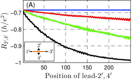
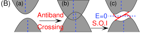
Figure 4: (Color online) (A). For the parameters used in Fig.1(A2), the 4-lead measurement of Hall resistances v.s. the position to measure at $E_{F}=0$. From top to bottom, the blue, red, green, and black lines are for the disorder strength $Dis=0$, $\Delta/8$, $\Delta/4$, and $\Delta/2$, respectively. Here the gap is $\Delta=0.16|t_{ab}|$. The results are calculated with the width of sample $W=70a$, by the average of 700 disorder configurations. (B). The schematic diagram of another method to realize twisting edge bands.

Finally, we should point out that though our results are obtained from an ideal model, the twisting edge bands can be found in some real systems. For example, supposing we initially have the two band system as shown in Fig.4(B-a), whose symmetry axis of upper band is shifted from that of the lower band. Then with the anti-band crossing [Fig.4(B-b)], the pseudo spin-orbital interaction may open a gap and leads to a twisting edge band [Fig.4(B-c)].

In conclusion, we have shown that, with a twisting edge bands, the system has both the topological protected and unprotected edge states. In such a system, the Hall resistance is not determined by the topological number alone. In particular, the Hall resistance depends the measure position even for a translationally invariant system.

Acknowledgments: This work was financially supported by NBRP of China (2012CB921303 and 2009CB929100), NSF-China under Grants Nos. 10821403, 10974236, and 11074174, and US-DOE under Grants No. DE-FG02- 04ER46124.

References

- (1) M. Z. Hasan and C. L. Kane, Rev. Mod. Phys. 82, 3045 (2010).
- (2) X. L. Qi and S. C. Zhang, Rev. Mod. Phys. 83, 1057 (2011).
- (3) F. D. M. Haldane, Phys. Rev. Lett. 61, 2015(1988).
- (4) C. L. Kane and E. J. Mele, Phys. Rev. Lett. 95, 226801 (2005); 95, 146802 (2005).
- (5) B. A. Bernevig, T. A. Hughes, and S. C. Zhang, Science 314, 1757 (2006);
- (6) M. Knig, S. Wiedmann, C. Brne, A. Roth, H. Buhmann, L. Molenkamp, X.-L. Qi, and S.-C. Zhang, Science 318, 766 (2007).
- (7) L. Fu, and C. L. Kane, Phys. Rev. B 76, 045302 (2007); D. Hsieh, D. Qian, L. Wray, Y. Xia, Y. S. Hor, R. J. Cava, and M. Z. Hasan, Nature (London) 452, 970 (2008); Y. Xia, D. Qian, D. Hsieh, L. Wray, A. Pal, H. Lin, A. Bansil, D. Grauer, Y. S. Hor, R. J. Cava, and M. Z. Hasan, Nat. Phys. 5, 398 (2009).
- (8) B. Zhou, H.-Z. Lu, R.-L. Chu, S.-Q. Shen, and Q. Niu, Phys. Rev. Lett. 101, 246807 (2008); M. Knig, H. Buhmann, L.W. Molenkamp, T. L. Hughes, C.-X.Liu, X. L. Qi, and S. C. Zhang, J. Phys. Soc. Jpn. 77, 031007 (2008); J. Linder, T. Yokoyama, and A. Sudb, Phys. Rev. B 80, 205401 (2009); Lu, H. Z., W.Y. Shan, W. Yao, Q. Niu, and S. Q. Shen, Phys. Rev. B 81, 115407 (2010).
- (9) C. Wu, B. A. Bernevig, and S. C. Zhang, Phys. Rev. Lett. 96, 106401 (2006); C. Xu, and J. E. Moore, Phys. Rev. B 73, 045322 (2006).
- (10) L. Fu, C. L. Kane, and E. J. Mele, Phys. Rev. Lett. 98, 106803 (2007).
- (11) Xuele Liu, Ziqiang Wang, X. C. Xie, and Yue Yu, Phys. Rev. B 83, 125105 (2011).
- (12) X. J. Liu, X. Liu, C. Wu, and J. Sinova, Phys. Rev. A 81, 033622 (2010).
- (13) D. J. Thouless, M. Kohmoto, M. P. Nightingale, and M. den. Nijs, Phys. Rev. Lett. 49, 405 (1982).
- (14) In the calculation of the transmission coefficients , we use the same method as in some references, e.g. W. Long, Q.-F. Sun, and J. Wang, Phys. Rev. Lett. 101, 166806 (2008); H. Jiang, S. Cheng, Q.-F. Sun, and X. C. Xie, Phys. Rev. Lett. 103, 036803 (2009).
- (15) Notice that this argument is not supported by the measurement for both the topological trivial system and normal topological system.