Kondo effect of an adatom in graphene and its scanning tunneling spectroscopy

Abstract

We study the Kondo effect of a single magnetic adatom on the surface of graphene. It was shown that the unique linear dispersion relation near the Dirac points in graphene makes it more easy to form the local magnetic moment, which simply means that the Kondo resonance can be observed in a more wider parameter region than in the metallic host. The result indicates that the Kondo resonance indeed can form ranged from the Kondo regime, to the mixed valence, even to the empty orbital regime. While the Kondo resonance displays as a sharp peak in the first regime, it has a peak-dip structure and/or an anti-resonance in the remaining two regimes, which result from the Fano resonance due to the significant background leaded by dramatically broadening of the impurity level in graphene. We also study the scanning tunneling microscopy (STM) spectra of the adatom and they show obvious particle-hole asymmetry when the chemical potential is tuned by the gate voltages applied to the graphene. Finally, we explore the influence of the direct tunneling channel between the STM tip and the graphene on the Kondo resonance and find that the lineshape of the Kondo resonance is unaffected, which can be attributed to unusual large asymmetry factor in graphene. Our study indicates that the graphene is an ideal platform to study systematically the Kondo physics and these results are useful to further stimulate the relevant experimental studies on the system.

I Introduction

The experimental realization of graphene Novoselov2004 ; Novoselov2005 composed of a monolayer of carbon atoms trigged a new wave to study the carbon-based materials, both from fundamental physics and applications. Beenakker2008 ; Neto2009 ; Peres2010 The graphene possesses perfect two-dimensional massless Dirac fermion behaviors, and the valence and conduction bands touch at two inequivalent Dirac points $K_{-}$ and $K_{+}$ at the corner of the Brillouin zone. Around the Dirac points the low-energy excitations are linear and the unique electronic structure leads to a number of unusual electronic correlation and transport properties of graphene. Beenakker2008 ; Neto2009 ; Peres2010 ; Peres2006 ; Ziegler2006 ; Nomura2007 ; Zhuang2009 ; Kotov2010 ; Jacob2010

For example, the localized magnetic moment on adatom with inner shell electrons in graphene behaves quite different to that in metals, a conventional Fermi liquid with a constant density of states near the Fermi surface. Anderson showed that in such a host the strongly interacting impurity ion can be in a magnetic state if the on-site interaction $U$ is sufficiently large and/or the hybridization $V$ between the impurity ion and the conduction electrons is sufficiently small. Anderson1961 Explicitly, it is required that the energy of the single occupancy states $\varepsilon_{d}$ is below the Fermi level $\mu$ but the energy of the double occupancy states, namely, $\varepsilon_{d}+U$, should be larger than $\mu$. Moreover, the magnetic regime was found to be symmetric around $y=(\mu-\varepsilon_{d})/U=0.5$. For details one can refer to the phase diagram given by the well-known Ref. [Anderson1961, ]. In contrast, when the host is graphene, the situation is dramatically different due to the linear density of states near the Dirac points. Uchoa2008 ; Cornaglia2009 ; Hu2011 Firstly, the magnetic phase diagram is not symmetric, it depends on that the impurity level $\varepsilon_{d}$ is above or below the Dirac points. Secondly and also most important difference is that the phase boundary is not symmetric around $y=0.5$ in both cases. When $\varepsilon_{d}$ is above the Dirac points, the magnetic state extends to $y<0$, which means that even the impurity level is located above the Fermi energy, it is possible that the localized magnetic moment exists. This is quite different to that in usual metallic host. In the other case that $\varepsilon_{d}$ is below the Dirac points, the phase boundary extends to $y>1$, which means that even the impurity is in the double occupancy state, it can be magnetized. It was realized that all these unusual features are due to the linear dispersion of the graphene around the Dirac points, and the impurity level is broadened dramatically by hybridization to cross the Fermi level. Uchoa2008

A direct consequence of the much wide magnetic regime is that the Kondo effect in graphene Sengupta2008 may exist in a more wide parameter regime than that in the usual metallic host in which the Kondo effect only exists in the Kondo regime, namely, $\epsilon_{d}/\Gamma\ll-0.5$, Goldhaber-Gordon1998 where $\Gamma$ is the effective tunneling coupling between the impurity and conduction electrons. Moreover, it is also interesting to explore what effect the dramatic broadening of the impurity level on the Kondo physics. This motivates us to study the Kondo effect of an adatom on the surface of the graphene sheet in a systematic way.

In this work the system we are interested in consists of the adatom, the graphene, and the tip on the top of the adatom, as shown in Fig. 1. As the first step, we explore the intrinsic equilibrium Kondo effect of the adatom as the conduction sea of electrons is limited to the graphene. The Kondo physics of the adatom generally depends on its explicit positions on the surface of the graphene. When the adatom is absorbed on the top of carbon atom, the situation is quite simple since the orbital degree of freedom is not involved in the case. However, when the adatom is located at the center of the honeycomb, a high symmetry position, the adatom hybridizes with the carbon atoms in both sublattices, Uchoa2009 ; Saha2010 ; Wehling2010a ; Wehling2010b ; Jacob2010 ; Uchoa2011 thus the orbital degree of freedom is involved which complicates the Kondo physics. For simplify, here we only focus on the first case and leave the latter one for the future study. When the Fermi energy is near the Dirac points, the Kondo effect is absent since a critical coupling strength must be satisfied for developing Kondo effect. Sengupta2008 ; Zhuang2009 ; Vojta2010 Once the Fermi energy is tuned to be away from the Dirac points, despite it is below or above the Dirac points, the Kondo resonance is found to exist in a wide parameter regime ranged from the Kondo regime to the mixed valence regime, even to the empty orbital regime. This is consistent with our intuition since the localized magnetic moment exists in a very wide parameter regime. When the system is in the Kondo regime, the Kondo resonance manifests as a sharp peak. This peak appears weaker and weaker when the impurity level becomes deeper and deeper. This is understandable since the broadening of the impurity level becomes weak due to the low density of states of the graphene near the Dirac points. When the system is in the mixed valence or empty orbital regimes, the Kondo resonance develops, however, it does not show a sharp peak but a peak-dip structure, even an anti-resonance, which is a typical Fano resonance behavior. Fano1961 ; Luo2004

In the next step, we consider a normal tip on the top of the adatom and the aim is to study the scanning tunneling microscopy (STM) spectra of the Kondo resonance of the adatom in graphene. We first turn off the direct tunneling between the tip and the graphene. The Kondo resonance shows asymmetric behaviors that depends on the position of the Fermi energy, namely, it is above or below the Dirac points. Moreover, the Kondo temperature strongly but asymmetrically depends on the explicit position of the Fermi energy which is in agreement with reported in the literature. Vojta2010 ; Zhu2011 Subsequently, we turn on the direct tunneling between the tip and the graphene to study its influence on the lineshape of the Kondo resonance, which also is more realistic case. It is somehow surprising that the lineshape is almost unaffect by the additional direct channel. This result in fact originates from the unusual large asymmetry factor in graphene.

The paper is organized as follows. In Sec. II we take the single-impurity Anderson model to describe the adatom on the surface of the graphene and derive transport formula by Keldysh nonequilibrium Green’s function theory. In Sec. III we solve numerically the equations obtained in a self-consistent way and discuss explicitly the Kondo effect in various situations including the cases of (i) the adatom plus the graphene, (ii) the adatom plus the graphene plus the tip, and (iii) the STM spectra with the direct channel between the tip and the graphene. Finally, a brief summary is devoted to Sec. IV.

II Model and Formalism

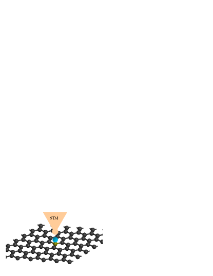
Figure 1: Schematic diagram of the STM measurement of a magnetic adatom absorbed on the top of a carbon atom site.

The Hamiltonian of a magnetic adatom on graphene with an STM tip consists of the following terms

$$H=H_{d}+H_{g}+H_{dg}+H_{t}+H_{dt}+H_{tg},$$ (1)

where

$$H_{d}=\sum_{\sigma}\varepsilon_{d}d_{\sigma}^{{\dagger}}d_{\sigma}+U\,d_{\sigma}^{{\dagger}}d_{\sigma}d_{\bar{\sigma}}^{{\dagger}}d_{\bar{\sigma}},$$ (2)

describes the magnetic adatom with the impurity level $\varepsilon_{d}$ and the on-site interaction $U$. Anderson1961 Here $d_{\sigma}^{{\dagger}}\left(d_{\sigma}\right)$ is a creation (annihilation) operator of localized electrons on magnetic adatom with spin $\sigma\left(=\uparrow,\downarrow\right)$ and $\bar{\sigma}=-\sigma$. The second term in Eq. (1) is the tight-banding Hamiltonian describing graphene, which can be written as in momentum space

$$H_{g}=-t\sum_{k\sigma}\left(\eta_{k}a_{k\sigma}^{\dagger}b_{k\sigma}+H.c.\right),$$ (3)

$a_{k\sigma}^{\dagger}\left(a_{k\sigma}\right)$ and $b_{k\sigma}^{\dagger}\left(b_{k\sigma}\right)$ are creation (annihilation) operators of electrons in sublattice A and B, respectively. $t$ is the hopping energy between the nearest-neighbor carbon atoms, $\eta_{k}=\sum_{{}_{i=1}}^{3}e^{i\vec{k}\cdot\vec{r}_{i}}\$ with $\vec{r}_{1}=a\vec{x},$ $\vec{r}_{2}=-\frac{a}{2}\vec{x}+\frac{\sqrt{3}a}{2}\vec{y}$, $\vec{r}_{3}=-\frac{a}{2}\vec{x}-\frac{\sqrt{3}a}{2}\vec{y}$, and $a\approx 1.42$ Å is the carbon-carbon spacing. Neto2009 The low-energy transport properties of graphene are mostly determined by the nature of spectrum around Dirac points $K_{\pm}$ at the corners of Brillouin zone, where the dispersion is $\varepsilon_{k}\approx\pm\upsilon_{F}|k|$, the sign $+\left(-\right)$ corresponds to the conduction (valence) band, and $\upsilon_{F}=3ta/2$ ($\approx 10^{6}$ m/s) is the Fermi velocity of Dirac electrons. The tip Hamiltonian is described by a normal metal

$$H_{t}=\sum_{k\sigma}\xi_{k}t_{k\sigma}^{{\dagger}}t_{k\sigma},$$ (4)

where $t_{k\sigma}^{{\dagger}}\left(t_{k\sigma}\right)$ represents the creation (annihilation) of an electron with energy $\xi_{k}$ on tip. The Hamiltonian

$$H_{dg}=\sum_{k\sigma}\left(V_{ka\sigma}a_{k\sigma}^{\dagger}+V_{kb\sigma}b_{k\sigma}^{\dagger}\right)d_{\sigma}+H.c.,$$ (5)

and

$$H_{dt}=\sum_{k\sigma}\left(V_{kt\sigma}t_{k\sigma}^{{\dagger}}d_{\sigma}+H.c.\right),$$ (6)

represent electrons tunneling from magnetic adatom to graphene and to STM tip, respectively. $V_{ka\sigma}$ $\left(V_{kb\sigma}\right)$ is the electron tunneling amplitude between magnetic adatom and sublattice A (B), and $V_{kt\sigma}$ is the tunneling amplitude between magnetic adatom and STM tip. If the adatom is adsorbed above the carbon atom in the sublattice A, thus $V_{ka\sigma}=V_{kg\sigma}$ and $V_{kb\sigma}=0$ or in the sublattice B, thus $V_{ka\sigma}=0$ and $V_{kb\sigma}=V_{kg\sigma}$. The direct tunneling Hamiltonian between graphene and the STM tip is described by

$$H_{tg}=\sum_{kk^{\prime}\sigma}T_{tg}\left(t_{k\sigma}^{\dagger}b_{k^{\prime}\sigma}+t_{k\sigma}^{\dagger}a_{k^{\prime}\sigma}\right)+H.c.,$$ (7)

where $T_{tg}$ is the hopping amplitude between the STM tip and graphene sheet.

In steady state, the current from the STM tip to the graphene sheet can be calculated by time-dependent occupancy number

$$I =-\frac{e}{2}\left(\left\langle\dot{N}_{t}\right\rangle-\left\langle\dot{N}_{g}\right\rangle\right)=-\frac{ie}{2\hbar}\left\langle\left[H,\left(N_{t}-N_{g}\right)\right]\right\rangle$$ (8)

$$=-\frac{e}{\hbar}\text{Re}\sum_{k\sigma}\left(V_{kg\sigma}^{\ast}G_{\sigma,gk\sigma}^{<}\left(t,t^{\prime}\right)-V_{kt\sigma}^{\ast}G_{\sigma,tk\sigma}^{<}\left(t,t^{\prime}\right)\right)$$

$$\hskip 28.45274pt-\frac{2e}{\hbar}\text{Re}\sum_{kk^{\prime}\sigma}T_{tg}^{\ast}G_{tk\sigma,gk^{\prime}\sigma}^{<}\left(t,t^{\prime}\right),$$

where $N_{t}=\sum_{k\sigma}t_{k\sigma}^{{\dagger}}t_{k\sigma}$ and $N_{g}=\sum_{k\sigma}c_{k\sigma}^{{\dagger}}c_{k\sigma}$. Here we use $c_{k\sigma}^{\dagger}$($c_{k\sigma}$) to denote the electron creation (annihilation) operator in the graphene sheet. The current is related to the lesser Green’s functions defined as $G_{\sigma,tk\sigma}^{<}\left(t,t^{\prime}\right)=i\left\langle t_{k\sigma}^{{\dagger}}\left(t^{\prime}\right)d_{\sigma}\left(t\right)\right\rangle,$ $G_{\sigma,gk\sigma}^{<}\left(t,t^{\prime}\right)=i\left\langle c_{k\sigma}^{\dagger}\left(t^{\prime}\right)d_{\sigma}\left(t\right)\right\rangle$ and $G_{tk\sigma,gk^{\prime}\sigma}^{<}\left(t,t^{\prime}\right)=i\left\langle c_{k^{\prime}\sigma}^{\dagger}\left(t^{\prime}\right)t_{k\sigma}\left(t\right)\right\rangle$. These Green’s functions can be calculated by the equations of motion (EOM) approach based on nonequilibrium Green’s functions theory. For a detail one can refer to Ref. [Jauho1994, ]. For simplify, we assume that the tunneling amplitudes $V_{kg\sigma}=V_{g}$ and $V_{kt\sigma}=V_{t}$ are independent on energy and spin. After some straightforward derivations, one can obtain the current formula

$$I =\frac{ie}{h}\sum_{\sigma}\int\left\{\left(G_{\sigma}^{r}\left(\varepsilon\right)-G_{\sigma}^{a}\left(\varepsilon\right)\right)[\Gamma_{t}\left(\varepsilon\right)f_{t}\left(\varepsilon\right)-\Gamma_{g}\left(\varepsilon\right)f_{g}\left(\varepsilon\right)]+\left(\Gamma_{t}\left(\varepsilon\right)-\Gamma_{g}\left(\varepsilon\right)\right)G_{\sigma}^{<}\left(\varepsilon\right)\right\}d\varepsilon$$ (9)

$$\hskip 28.45274pt+\frac{2e}{h}\int\left(f_{t}\left(\varepsilon\right)-f_{g}\left(\varepsilon\right)\right)\left[\Pi\left(\varepsilon\right)-\Phi\left(\varepsilon\right)\sum_{\sigma}\text{Im}(G_{\sigma}^{r}\left(\varepsilon\right))\right]d\varepsilon,$$

where $G_{\sigma}^{<,r,a}\left(\varepsilon\right)$ is the Fourier transformation of time-order Green’s function $G_{\sigma}^{<,r,a}\left(t,t^{\prime}\right)$ defined by $G_{\sigma}^{<}\left(t,t^{\prime}\right)=i\left\langle d_{\sigma}^{{\dagger}}\left(t^{\prime}\right)d_{\sigma}\left(t\right)\right\rangle$, $G_{\sigma}^{r\left(a\right)}\left(t,t^{\prime}\right)=\mp i\theta\left(\pm t\mp t^{\prime}\right)\left\langle\{d_{\sigma}\left(t\right),d_{\sigma}^{{\dagger}}\left(t^{\prime}\right)\}\right\rangle.$ $\Gamma_{g}\left(\varepsilon\right)=\pi\left|V_{g}\right|^{2}\rho_{g}\left(\varepsilon\right)$ and $\Gamma_{t}\left(\varepsilon\right)=\pi\left|V_{t}\right|^{2}\rho_{t}\left(\varepsilon\right)$ are the couplings between the magnetic adatom to the graphene and to the tip, respectively. $\Pi\left(\varepsilon\right)=\pi\left|T_{tg}\right|^{2}\rho_{t}\left(\varepsilon\right)\rho_{g}\left(\varepsilon\right)$ corresponds to hopping from the tip to graphene and vice versa. $\Phi\left(\varepsilon\right)=\sqrt{\pi\Pi\left(\varepsilon\right)\Gamma_{g}\left(\varepsilon\right)\Gamma_{t}\left(\varepsilon\right)}$ is related to the interference between the different tunneling channels. $\rho_{g}\left(\varepsilon\right)$ and $\rho_{t}\left(\varepsilon\right)$ are the density of states of graphene and STM tip, respectively. The density of states for tip is simplified with a constant $\rho_{t}\left(\varepsilon\right)=1/2D$, and the density of states for graphene can be evaluated with $\rho_{g}\left(\varepsilon\right)=\Theta(D-|\varepsilon|)|\varepsilon|/D^{2}$. Wehling2010b Here $D$ is the half-width of conduction band. For convenience, we take $\Gamma_{g}(\varepsilon)=\Gamma_{0}|\varepsilon|/{D}$ where $\Gamma_{0}=\pi|V_{g}|^{2}/D$. $f_{g}\left(\varepsilon\right)$ and $f_{t}\left(\varepsilon\right)$ are the Fermi distribution functions of graphene and the STM tip. The nonequilibrium Kondo effect can be discussed by differential conductance near the Fermi level. Thus, our final task to calculate the current is to solve the Green’s functions involved.

The equations for the retarded Green’s functions and the lesser Green’s functions can be derived by the Schwinger-Keldysh perturbation formalism Mahan1993 ; Niu1999 ; Swirkowicz2003 ; Krawiec2004 which are given by, respectively,

$$G_{\sigma}^{r}\left(\varepsilon\right)=g_{d}^{r}(\varepsilon)\left(1+\left\langle\left\langle\left[d_{\sigma},H_{I}\right];d_{\sigma}^{\dagger}\right\rangle\right\rangle_{\varepsilon}^{r}\right),$$ (10)

$$G_{\sigma}^{<}\left(\varepsilon\right)=g_{d}^{<}(\varepsilon)\left(1+\left\langle\left\langle\left[d_{\sigma},H_{I}\right];d_{\sigma}^{\dagger}\right\rangle\right\rangle_{\varepsilon}^{a}\right)$$

$$\hskip 56.9055pt+g_{d}^{r}\left(\varepsilon\right)\left\langle\left\langle\left[d_{\sigma},H_{I}\right];d_{\sigma}^{\dagger}\right\rangle\right\rangle_{\varepsilon}^{<},$$ (11)

where $g_{d}^{r}(\varepsilon)=1/\left(\varepsilon-\varepsilon_{d}+i0^{+}\right)$ and $g_{d}^{<}\left(\varepsilon\right)=i\pi f(\varepsilon)\delta(\varepsilon-\varepsilon_{d})$ are the noninteracting retarded and lesser Green’s functions for the isolated magnetic adatom. In the above expressions the $H_{I}=Ud_{\sigma}^{{\dagger}}d_{\sigma}d_{\bar{\sigma}}^{{\dagger}}d_{\bar{\sigma}}+H_{dg}+H_{dt}$ includes the on-site Coulomb repulsion term on the adatom and the tunneling terms. While the first term will lead to higher-order Green’s functions contained into $\left\langle\left\langle\left[d_{\sigma},H_{I}\right];d_{\sigma}^{\dagger}\right\rangle\right\rangle_{\varepsilon}^{r(a,<)}$ by using Zubarev notations, Zubarev1960 the remaining two terms only lead to the hybridization effect. Furthermore, the derivation of the EOM of the higher-order Green’s function will also introduce more higher-order Green’s functions, which have to be truncated in order to close the hierarchy of the EOM of the successive Green’s functions. Here we truncate this hierarchy of EOM by using Lacroix’s scheme, Lacroix1981 which is shown to be enough to capture the Kondo resonance, even at zero temperature. Lacroix1981 ; Luo1999 Since the derivation is standard we directly write down the Green’s functions in the infinite-U limit as follows

$$G_{\sigma}^{r}\left(\varepsilon\right)=\frac{1-\left\langle n_{\bar{\sigma}}\right\rangle-A_{\bar{\sigma}}\left(\varepsilon\right)}{\varepsilon-\varepsilon_{d}-\Sigma\left(\varepsilon\right)\left(1-A_{\bar{\sigma}}\left(\varepsilon\right)\right)-B_{\bar{\sigma}}\left(\varepsilon\right)},$$ (12)

and

$$G_{\sigma}^{<}\left(\varepsilon\right)=G_{\sigma}^{r}\left(\varepsilon\right)\frac{\Sigma^{<}\left(\varepsilon\right)\left(1-A_{\bar{\sigma}}\left(\varepsilon\right)\right)+B_{\bar{\sigma}}^{<}\left(\varepsilon\right)-A_{\bar{\sigma}}^{<}\left(\varepsilon\right)\left(G_{\sigma}^{a}\left(\varepsilon\right)^{-1}+\Sigma\left(\varepsilon\right)\right)}{1-\left\langle n_{\bar{\sigma}}\right\rangle-A_{\bar{\sigma}}\left(\varepsilon\right)}G_{\sigma}^{a}\left(\varepsilon\right).$$ (13)

Here the self-energy $\Sigma\left(\varepsilon\right)=\frac{-i\Gamma\left(\varepsilon\right)-\Phi\left(\varepsilon\right)-\left(\Phi\left(\varepsilon\right)\right)^{\ast}}{1+\pi\Pi\left(\varepsilon\right)},$ $\Gamma\left(\varepsilon\right)=\Gamma_{g}\left(\varepsilon\right)+\Gamma_{t}\left(\varepsilon\right)$ and $\Sigma^{<}\left(\varepsilon\right)=\frac{i\Xi_{1}\left(\varepsilon\right)+\Omega\left(\varepsilon\right)}{1+\pi\Pi\left(\varepsilon\right)}$, the average of occupation $\left\langle n_{\bar{\sigma}}\right\rangle=-\frac{1}{\pi}\int\frac{\Xi_{1}\left(\varepsilon\right)}{\Gamma\left(\varepsilon\right)}\text{Im}(G_{\bar{\sigma}}^{r}\left(\varepsilon\right))d\varepsilon,$ and

$$A_{\bar{\sigma}}\left(\varepsilon\right)=\frac{1}{\pi}\int\frac{g\left(\varepsilon,\varepsilon^{\prime}\right)\left(\Xi_{1}\left(\varepsilon^{\prime}\right)+i\Omega\left(\varepsilon^{\prime}\right)\right)(G_{\bar{\sigma}}^{r}\left(\varepsilon^{\prime}\right))^{\ast}}{1+\pi\Pi\left(\varepsilon^{\prime}\right)}d\varepsilon^{\prime},$$ (14)

$$B_{\bar{\sigma}}\left(\varepsilon\right) = \frac{1}{\pi}\int g\left(\varepsilon,\varepsilon^{\prime}\right)\Xi_{1}\left(\varepsilon^{\prime}\right)d\varepsilon^{\prime}+$$ (15)

$$\frac{i}{\pi}\int g\left(\varepsilon,\varepsilon^{\prime}\right)\left(\Xi_{2}\left(\varepsilon^{\prime}\right)+\Xi_{3}\left(\varepsilon^{\prime}\right)\right)(G_{\bar{\sigma}}^{r}\left(\varepsilon^{\prime}\right))^{\ast}d\varepsilon^{\prime}$$

$$+\frac{1}{\pi}\int\frac{g\left(\varepsilon,\varepsilon^{\prime}\right)\Xi_{1}\left(\varepsilon^{\prime}\right)\Phi\left(\varepsilon^{\prime}\right)(G_{\bar{\sigma}}^{r}\left(\varepsilon^{\prime}\right))^{\ast}}{1+\pi\Pi\left(\varepsilon^{\prime}\right)}d\varepsilon^{\prime},$$

$$A_{\bar{\sigma}}^{<}\left(\varepsilon\right)=\frac{i\Xi_{1}\left(\varepsilon\right)\text{Re}\left(G_{\bar{\sigma}}^{r}\left(\varepsilon\right)\right)+i\Omega\left(\varepsilon\right)\text{Im}\left(G_{\bar{\sigma}}^{r}\left(\varepsilon\right)\right)}{1+\pi\Pi\left(\varepsilon\right)},$$ (16)

$$B_{\bar{\sigma}}^{<}\left(\varepsilon\right) = i\Xi_{1}\left(\varepsilon\right)+i\left(\Xi_{2}\left(\varepsilon\right)+\Xi_{3}\left(\varepsilon\right)\right)\text{Im}\left(G_{\bar{\sigma}}^{r}\left(\varepsilon\right)\right)$$ (17)

$$-i\Xi_{1}\left(\varepsilon\right)\frac{\Phi\left(\varepsilon\right)\text{Im}\left(G_{\bar{\sigma}}^{r}\left(\varepsilon\right)\right)}{1+\pi\Pi\left(\varepsilon\right)},$$

where $g\left(\varepsilon,\varepsilon^{\prime}\right)=1/\left(\varepsilon-\varepsilon^{\prime}+i0^{+}\right)$, $\Omega\left(\varepsilon\right)=\Phi\left(\varepsilon\right)f_{g}\left(\varepsilon\right)+\left(\Phi\left(\varepsilon\right)\right)^{\ast}f_{t}\left(\varepsilon\right),$ $\Xi_{1}\left(\varepsilon\right)=f_{g}\left(\varepsilon\right)\Gamma_{g}\left(\varepsilon\right)+f_{t}\left(\varepsilon\right)\Gamma_{t}\left(\varepsilon\right),$ $\Xi_{2}\left(\varepsilon\right)=f_{g}\left(\varepsilon\right)\Gamma_{g}\left(\varepsilon\right)\Gamma_{g}\left(\varepsilon\right)+f_{t}\left(\varepsilon\right)\Gamma_{t}\left(\varepsilon\right)\Gamma_{t}\left(\varepsilon\right),$ $\Xi_{3}\left(\varepsilon\right)=\Gamma_{g}\left(\varepsilon\right)\Gamma_{t}\left(\varepsilon\right)\left(f_{gt}\left(\varepsilon\right)+f_{tg}\left(\varepsilon\right)\right)$ with $f_{gt}\left(\varepsilon\right)=f_{g}\left(\varepsilon\right)\left(1-f_{t}\left(\varepsilon\right)\right)$. At the hand of the above expressions, we can calculate numerically the Green’s function $G_{\sigma}^{r}\left(\varepsilon\right)$ and $G_{\sigma}^{a}\left(\varepsilon\right)=\left(G_{\sigma}^{r}\left(\varepsilon\right)\right)^{\ast}$ in a self-consistent way, and further the lesser Green function $G_{\sigma}^{<}\left(\varepsilon\right)$. Finally, we obtain the current $I$ by Eq. (9).

III Numerical results and discussions

In the following numerical calculation, several input parameters are tuned in order to study the system in different physical situations. The atomic level $\epsilon_{d}$ is changed to study the different regimes ranged from the Kondo regime, to the mixed valence regime, even to the empty orbital regime. Goldhaber-Gordon1998 The chemical potential of graphene $\mu$ can be tuned by gate-voltage, which makes the Fermi level is located at ($\mu=0$), above ($\mu>0$) or below ($\mu<0$) the Dirac points. The different chemical potential will lead to quite different physics, as shown below. The voltage bias $V_{sd}$ is also applied between STM tip and graphene sheet to calculate the differential conductance. For convenience, we take $\Gamma_{0}$ as the units of energy in the calculations. As a systematic study, we first to calculate the Kondo effect of the adatom plus the graphene when the STM tip is omitted. The aim is to explore the influence of the linear dispersion around the Dirac points to the Kondo effect and compare it with the adatom on normal metal surface. Subsequently, we consider the influence of the STM tip and explore the Kondo resonance when both the normal metal and the graphene are coupled to the adatom. Finally, we turn on the direct channel between the STM tip and the Graphene and check its effect in the tunneling spectroscopy, which is more closely related to the experiment.

III.1 Kondo effect of the adatom without the STM tip

Figure 2: The Kondo resonance of the magnetic adatom on graphene with different atomic levels ranged from the empty orbital regime to the Kondo regime. From (a) to (f) the atomic level is $\epsilon_{d}=2.5\Gamma_{0}$, $1.5\Gamma_{0}$, $0.5\Gamma_{0}$, 0, $-0.5\Gamma_{0}$, $-1.5\Gamma_{0}$. The inset in each panel is enlarged view around the Kondo resonance. The chemical potential is $\mu=0.5\Gamma_{0}$, the temperature $T=0.00005\Gamma_{0}$, and the half-bandwidth $D=5\Gamma_{0}$.

Figure 3: The same as Fig. 2 but for $\mu=-0.5\Gamma_{0}$. From (a) to (f) the atomic level is $\varepsilon_{d}=1.5\Gamma_{0}$, $0.5\Gamma_{0}$, 0, $-0.5\Gamma_{0}$, $-1.5\Gamma_{0}$, $-2.5\Gamma_{0}$.

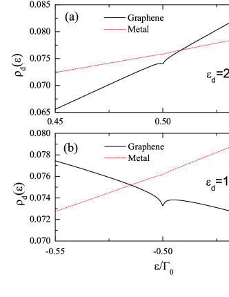
Figure 4: Comparison between the density of states around the Fermi level in the empty orbital regime for the metallic (red dashed lines) and the graphene (solid lines) hosts. (a) $\mu=0.5\Gamma_{0}$, $\varepsilon_{d}=2.5\Gamma_{0}$, and (b) $\mu=-0.5\Gamma_{0}$, $\varepsilon_{d}=1.5\Gamma_{0}$.

In order to explore the effect of the linear dispersion around the Dirac points, we first the system composed of the magnetic adatom plus the graphene and omit the STM tip. As pointed out by Uchoa et al., Uchoa2008 it is more easier to form the local moment for the magnetic impurity on the surface of the graphene than in the normal metal host. This conclusion has a direct consequence that one can observe the Kondo resonance in a more wider parameter region for the former than the latter one. This is really true as shown in Figs. 2 and 3 where we show the local density of states of the adatom given by $\rho_{d}(\varepsilon)=-\frac{1}{\pi}\text{Im}G^{r}_{\sigma}(\varepsilon)$. In Fig. 2 we consider $\mu=0.5\Gamma_{0}$, namely, the Fermi level is above the Dirac points. We change the atomic level from the empty orbital regime, as shown in Fig. 2(a) to the Kondo regime [see Fig. 2(f)], around the Fermi level the local density of states show special feature, i.e., the Kondo resonance, although their shapes are quite different. In the Kondo regimes, the Kondo resonance exhibits as a sharp peak around the Fermi level but one should notice that with increasing the atom level the peak becomes gradually asymmetric, which is quite obvious in Fig. 2(d) for $\varepsilon_{d}=0$. Continuing to change the atomic level to $\varepsilon_{d}=0.5\Gamma_{0}$, the Kondo resonance has a typical peak-dip structure. Finally, we move the atomic level to the empty orbital regimes, the Kondo effect manifests as an anti-resonance, which is clearly seen from the inset of Fig. 2(a) and (b). These features are nothing but the Kondo resonance. They can be understood based on our previous work. Luo2004 In such a system, the Kondo resonance results from the coherent supposition between the Kondo peak and the broadening of the impurity level due to the hybridization with the conduction electron. In the Kondo regime, the broadening of the impurity level is quite weak around the Fermi level so the Kondo resonance shows as a sharp peak. When the system approaches to the mixed valence regime, the broadening of the impurity level becomes more and more sizeable and as a result, the Kondo peak distorts gradually due to the interference, and finally it becomes an anti-resonance when the system is in the empty orbital regime since in this case the Fermi level is located at the left-hand side of the broadening impurity level. The essential reason that the Kondo effect can exist in a wide parameter region is the impurity level is broadened extensively due to the linear density of states of the graphene around the Dirac points. Therefore, the adatom on the surface of the graphene provides an idea system to study the Kondo effect in various parameter spaces. The same physics has been observed when the Fermi level is below the Dirac points, as shown in Fig. 3(a)-(f).

To confirm above observation, we compare the local density of states around the Fermi level for the adatom on graphene and on metal surface in the empty orbital regime, as show in Fig. 4. For metal host, one cannot observe any feature, which is in contrast to that in the graphene, where an obvious anti-resonance exists. The results are true either the chemical potential is above or below the Dirac points.

III.2 Kondo Effect of the adatom with the STM tip

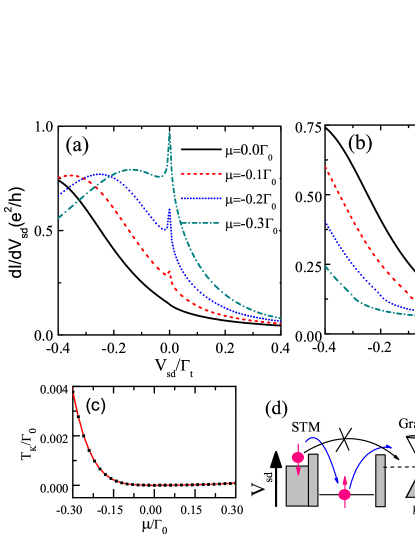
Figure 5: The Kondo resonance around the zero bias varies with the chemical potential (a) $\mu<0$ and (b) $\mu>0$. (c) The Kondo temperature $T_{k}$ versus the chemical potential $\mu$. The other parameters used are $\epsilon_{d}=-\Gamma_{0}$ where $\Gamma_{t}=0.1\Gamma_{0}$, $T_{tg}=0$ and $D=5\Gamma_{0}$. (d) shows schematically the cotunneling processes with the chemical potential $\mu<0$ and $\mu>0$, respectively.

When the STM tip is considered, the adatom couples with two baths, one is the STM tip which is a normal metal with a constant density of states, as studied in the conventional Kondo physics. The other is the graphene which has a linear density of states around the Dirac points. We first study the nonequilibrium Kondo effect in this case. Therefore, we omit the direct channel between the STM tip and the graphene. In the calculations, the coupling between the adatom and tip is taken with $\Gamma_{t}=0.1\Gamma_{0}$. Fig. 5 shows the differential conductance around the zero bias. When the chemical potential $\mu$ is tuned to meet the Dirac points, the curve at the zero bias shows a kink but no visible Kondo peak, which is a consequence of the zero density of states at the Dirac points. When the chemical potential $\mu$ is tuned to be away from the Dirac points, either above or below the Dirac points, the zero bias peak occurs, which shows the Kondo effect. When the chemical potential below the Dirac points, the more larger $|\mu|$ is, the more wider the peak is. This is easy to understand since the larger $\mu$ means the larger density of states at the side of graphene. When $\mu$ is above the Dirac points, the width of the Kondo resonance keeps almost unchange (see Fig. 5(c)), which also can be obtained from the chemical potential dependent Kondo temperature.Zhu2011 However, when $\mu$ is below the Dirac points, the Kondo temperature $T_{K}$ shows obvious dependence on $\mu$. As a result, the Kondo temperature is obvious asymmetric, which is consistent with that reported in the literature. Vojta2010 ; Zhu2011 This is due to the fact of the particle-hole asymmetry in graphene. In addition, one also notes that in both cases the curves show a kink when the bias scans through the Dirac points.

III.3 Scanning tunneling spectroscopy with direct channel

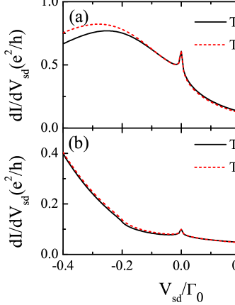
Figure 6: The Kondo resonance around the zero bias with and without the direct tunneling $T_{tg}$ channel for two cases (a) $\mu=-0.2\Gamma_{0}$ and (b) $\mu=0.2\Gamma_{0}$. We take $\varepsilon_{d}=-\Gamma_{0}$ and $T_{tg}=0.2\Gamma_{0}$. The other parameters used are the same as Fig. 5.

In this subsection we discuss the scanning tunneling spectroscopy of the adatom on the surface of graphene by switching on the direct tunneling channel between the STM tip and graphene, a more realistic case in experiments. Due to the additional direct channel, one may expect that the STM spectroscopy should be changed dramatically leaded by the interference between the direct and the indirect channels, as usually observed in a system with the adatom on the surface of the normal metals. Madhavan1998 However, the result is somehow surprising, as shown in Fig. 6. In comparison to the spectroscopy without the direct channel, except for the amplitudes, the shape almost keeps unchanged for both $\mu>0$ and $\mu<0$. To check the underlying physics of this result, let us recall the Fano resonance theory. Fano1961 In the STM case, due to the adatom scattering and its interference with the direction channel, the differential conductance of the conduction electron can be written as Luo2004

$$\frac{dI}{dV}\propto(q^{2}-1)\text{Im}\,G(\varepsilon)-2q\text{Re}\,G(\varepsilon),$$ (18)

where $G(\varepsilon)$ denotes the adatom Green’s function and $q\approx-\text{Re}\,g(\varepsilon)/\text{Im}\,g(\varepsilon)$ is the Fano asymmetry factor. Here $g(\varepsilon)$ is the graphene Green’s function with $\text{Re}\,g(\varepsilon)=(\varepsilon/D^{2})\ln|\varepsilon^{2}/(D^{2}-\varepsilon^{2})|$ and $\text{Im}\,g(\varepsilon)=-\pi|\varepsilon|/D^{2}\Theta(D-|\varepsilon|)$. Thus the $q$ factor is $2\,\text{sgn}(\mu)/\pi\ln|\mu|/D$ near the Fermi level. Wehling2010b For graphene, $D\sim 6\text{eV}$ (Ref. [Wehling2007, ]) and if $|\mu|$ maximally is in the order of $0.1\text{eV}$, so $|q|\gtrsim 6$. That means that the first term in Eq. (18) dominates the second term, as a result, the $dI/dV$ has the almost same profile as $\text{Im}G(\varepsilon)$, the local density of states of the adatom. This is the reason that the shapes of the Kondo resonance around the zero bias is almost same despite the direct channel is switched on or off.

IV Summary

In summary, we study systematically the Kondo effect of a magnetic adatom on the surface of graphene and its STM spectra. The main conclusion is that the Kondo resonance can exist in a much wide parameter region ranged from the Kondo regime, to the mixed valence regime, even to the empty orbital regime. In the mixed valence or the empty orbital regimes the Kondo resonance show specially lineshape due to the Fano resonance since in these regimes the broadening of the impurity level provides a significant background. The STM spectra have a particle-hole asymmetry when the chemical potential in graphene is tuned by the gate voltages. Furthermore, it is found that the direct tunneling channel between the STM tip and graphene has no obvious effect on the lineshape of the Kondo resonance around the zero bias, which is a consequence of the unusual large asymmetry factor in graphene host. The rich behaviors of the Kondo resonance obtained indicate that the graphene is an ideal platform to study the Kondo physics and these results are useful to further stimulate the relevant experimental works in this system.

V Acknowledgement

Supported from CMMM of Lanzhou University, the NSF, the national program for basic research and the fundamental research funds for the central universities of China is acknowledged.

References

- (1) K. S. Novoselov, A. K. Geim, S. V. Morozov, D. Jiang, Y. Zhang, S. V. Dubonos, I. V. Grigorieva, and A. A. Firsov, Science 306, 666 (2004).
- (2) K. S. Novoselov, A. K. Geim, S. V. Morozov, D. Jiang, M. I. Katsnelson, I. V. Grigorieva, S. V. Dubonos, and A. A. Firsov, Nature 438, 197 (2005).
- (3) Beenakker, C. W. J. Colloquium: Andreev reflection and Klein tunneling in graphene. Rev. Mod. Phys. 80, 1337 (2008).
- (4) A. H. Castro Neto, F. Guinea, N. M. R. Peres, K. S. Novoselov, and A. K. Geim, Rev. Mod. Phys. 81, 109 (2009).
- (5) N. M. R. Peres, Rev. Mod. Phys. 82, 2673 (2010).
- (6) N. M. R. Peres, F. Guinea, and A. H. Castro Neto, Phys. Rev. B 73, 125411 (2006).
- (7) K. Ziegler, Phys. Rev. Lett. 97, 266802 (2006).
- (8) K. Nomura and A. H. MacDonald, Phys. Rev. Lett. 98, 076602 (2007).
- (9) H.-B. Zhuang, Q.-f Sun, and X. C. Xie, EPL 86, 58004 (2009).
- (10) V. N. Kotov, B. Uchoa, V. M. Pereira, A. H. C. Neto, and F. Guinea, arxiv:1012.3484 (2010).
- (11) D. Jacob and G. Kotliar, Phys. Rev. B 82, 085423 (2010).
- (12) P. W. Anderson, Phys. Rev. 124, 41 (1961).
- (13) B. Uchoa, V. N. Kotov, N. M. R. Peres, and A. H. Castro Neto, Phys. Rev. Lett. 101, 026805 (2008).
- (14) P. S. Cornaglia, G. Usaj, and C. A. Balseiro, Phys. Rev. Lett. 102, 046801 (2009).
- (15) F. M. Hu, Tianxing Ma, Hai-Qing Lin, and J. E. Gubernatis, Phys. Rev. B 84, 075414 (2011).
- (16) K. Sengupta and G. Baskaran, Phys. Rev. B 77, 045417 (2008).
- (17) D. Goldhaber-Gordon, J. Göres, M. A. Kastner, H. Shtrikman, D. Mahalu, and U. Meirav, Phys. Rev. Lett. 81, 5225 (1998).
- (18) B. Uchoa, L. Yang, S. W. Tsai, N. M. R. Peres, and A. H. Castro Neto, Phys. Rev. Lett. 103, 206804 (2009).
- (19) K. Saha, I. Paul, and K. Sengupta, Phys. Rev. B 81, 165446 (2010).
- (20) T. O. Wehling, A. V. Balatsky, M. I. Katsnelson, A. I. Lichtenstein, and A. Rosch, Phys. Rev. B 81, 115427 (2010).
- (21) T. O. Wehling, H. P. Dahal, A. I. Lichtenstein, M. I. Katsnelson, H. C. Manoharan, and A. V. Balatsky, Phys. Rev. B 81, 085413 (2010).
- (22) B. Uchoa, T. G. Rappoport, and A. H. Castro Neto, Phys. Rev. Lett. 106, 016801 (2011).
- (23) M. Vojta, L. Fritz, and R. Bulla, EPL 90, 27006 (2010).
- (24) U. Fano, Phys. Rev. 124, 1866 (1961).
- (25) H. G. Luo, T. Xiang, X. Q. Wang, Z. B. Su, and L. Yu, Phys. Rev. Lett. 92, 256602 (2004); 96, 019702 (2006).
- (26) Z.-G. Zhu, and J. Berakdar, Phys. Rev. B 84, 165105 (2011).
- (27) A. P. Jauho, N. S. Wingreen and Y. Meir, Phys. Rev. B 50, 5528 (1994).
- (28) G. D. Mahan, Many-Particle Systems, 2nd ed. (Plenum Press, New York, 1993).
- (29) C. Niu, D.L. Lin, and T.H. Lin, J. Phys.: Condens. Matter 11, 1511 (1999).
- (30) R. Świrkowicz, J. Barnaś, and M. Wilczyński, Phys. Rev. B 68, 195318 (2003).
- (31) M. Krawiec and K. I. Wysokiński, Supercond. Sci. Technol. 17, 103-112 (2004).
- (32) D. N. Zubarev, Usp. Fiz. Nauk 71, 71 (1960) [Sov. Phys. Usp. 3, 320 (1960)].
- (33) C. Lacroix, J. Phys. F 11, 2389 (1981).
- (34) H.-G. Luo, Z.-J. Ying and S.-J. Wang, Phys. Rev. B 59, 9710 (1999).
- (35) V. Madhavan, W. Chen, T. Jamneala, M. F. Crommie, and N. S. Wingreen, Science 280, 567 (1998).
- (36) T. O. Wehling, A. V. Balatsky, M. I. Katsnelson, A. I. Lichtenstein, K. Scharnberg, and R. Wiesendanger, Phys. Rev. B 75, 125425 (2007).