Target Identification Using Dictionary Matching of Generalized Polarization Tensors

Abstract

The aim of this paper is to provide a fast and efficient procedure for (real-time) target identification in imaging based on matching on a dictionary of precomputed generalized polarization tensors (GPTs). The approach is based on some important properties of the GPTs and new invariants. A new shape representation is given and numerically tested in the presence of measurement noise. The stability and resolution of the proposed identification algorithm is numerically quantified.

Mathematics Subject Classification (MSC2000): 35R30, 35B30

Keywords: generalized polarization tensors, target identification, shape representation, stability analysis

1 Introduction

With each domain and material parameter, an infinite number of tensors, called the Generalized Polarization Tensors (GPTs), is associated. The concept of GPTs was introduced in [8, 6]. The GPTs contain significant information on the shape of the domain [9]. It occurs in several interesting contexts, in particular, in low-frequency scattering [17, 6], asymptotic models of dilute composites (see [21] and [13]), in invisibility cloaking in the quasi-static regime [10] and in potential theory related to certain questions arising in hydrodynamics [22].

Another important use of this concept is for imaging diametrically small inclusions from boundary measurements. In fact, the GPTs are the basic building blocks for the asymptotic expansions of the boundary voltage perturbations due to the presence of small conductivity inclusions inside a conductor [18, 16, 8]. Based on this expansion, efficient algorithms to determine the location and some geometric features of the inclusions were proposed. We refer to [6, 7] and the references therein for recent developments of this theory.

In [11], a recursive optimal control scheme to recover fine shape details of a given domain using GPTs is proposed. In [4], it is shown that high-frequency oscillations of the boundary of a domain are only contained in its high-order GPTs. Moreover, by developing a level set version of the recursive optimization scheme, it is also shown that the GPTs can capture the topology of the domain. An efficient algorithm for computing the GPTs has been presented in [15].

The aim of this paper is to show that the GPTs can be used for target identification from imaging data. In fact, the GPTs can be accurately obtained from multistatic measurements by solving a linear system. Based on this, we design a fast algorithm which identifies a target using a dictionary of precomputed GPTs data. We first provide a stability analysis for the reconstruction of the GPTs in the presence of measurement noise which quantifies the ill-posedness of the imaging problem. Then, suppose that we have a dictionary which is a collection of standard shapes (for example alphabetic letters or flowers). Our aim is to identify from imaging data a shape which is obtained from one element of the dictionary after some rotation, scaling and translation. We design a dictionary matching procedure which operates directly in the GPTs data. Our procedure is based on some important properties of the GPTs and new invariants. We test the robustness of our procedure with respect to a measurement noise in the imaging data. Our approach is quite natural since it uses geometric quantities obtained from the imaging data by simply inverting a linear system. Moreover, there is an infinite number of invariants associated with the GPTs. Furthermore, for a given dictionary, the GPT-based representation may lead to better distinguishibility between the dictionary elements.

Over the last decades, a considerable amount of work has been devoted to nonlinear optimization techniques for solving the imaging problem; see, for instance, [19, 23, 25] and the references therein. More recently, new regularized optimal control formulations for target imaging have been proposed in [1, 3]. As far as we know, our approach in this paper provides for the first time an alternative approach to solving the full inverse problem for target identification and characterization. It opens a way for real-time target identification and tracking algorithms in wave imaging.

The paper is organized as follows. In section 2, we introduce a particular linear combination of the GPTs to obtain what we call the contracted GPTs (CGPTs) [10]. In Section 3, we investigate the reconstruction of contracted GPTs, defined in (2.14)–(2.17) below, from the multistatic response matrix of a conductivity problem. We also consider the effect of the presence of measurement noise in the MSR on the reconstruction of the CGPTs. Given a signal-to-noise ratio, we determine the statistical stability in the reconstruction of the CGPTs, and show that such inverse problem is exponentially unstable. This is the well-known ill-posedness of the inverse conductivity problem. In section 4 it is shown that the CGPTs have some nice properties, such as simple rotation and translation formulas, simple relation with shape symmetry, etc. More importantly, we derive new invariants for the CGPTs. One of the matching algorithms presented in section 5 is based on those invariants. Section 6 presents a variety of numerical results for the target identification problem and shows the viability of the proposed procedure.

2 Structure of the Multistatic Response Matrix

The first part of this paper is to reconstruct CGPTs from the multistatic response (MSR) matrix, which measures the change in potential field due to a conductivity inclusion. In this section, we present the mathematical model for MSR and write it in terms of the CGPTs associated to the conductivity inclusion.

We consider a two dimensional conductivity medium with uniform conductivity equal to one, except in an inclusion where the conductivity is $\kappa>1$; we denote by $\lambda$ the contrast of this inclusion, that is, $\lambda=(\kappa+1)/(2(\kappa-1))$. Let $D=z+\delta B=\{x=z+\delta y~{}|~{}y\in B\}$ model the conductivity inclusion. Here, $B$ is some $\mathcal{C}^{2}$ and bounded domain in $\mathbb{R}^{2}$ whose typical length scale is of order one; $z$ is a point in $\mathbb{R}^{2}$ and is taken here to be an estimation of the location of the inclusion; $\delta$ is the typical length scale of the inclusion. We refer to [14, 6] for efficient location search algorithms and to [2] for correcting the effect of measurement noise on the localization procedure.

The MSR matrix is constructed as follows. Let $\{x_{r}\}_{r=1}^{N_{r}}$ and $\{x_{s}\}_{s=1}^{N_{s}}$ model a set of electric potential point detectors and electric point sources. We assume in this paper that the two sets of locations coincide and $N_{r}=N_{s}=N$. The MSR matrix $\mathbf{V}$ is an $N$-by-$N$ matrix whose $rs$-element is the difference of electric potentials with and without the conductivity inclusions:

$$V_{rs}=u_{s}(x_{r})-\Gamma_{s}(x_{r}),\quad r,s=1,\ldots,N.$$ (2.1)

Here, $\Gamma_{s}(x)=\Gamma(x-x_{s})$ and $\Gamma(x)=\frac{1}{2\pi}\log|x|$ is the fundamental solution of the Laplace equation in $\mathbb{R}^{2}$, and $u_{s}(x)$ is the solution to the transmission problem

$$\left\{\begin{aligned} \nabla\cdot(1+(\kappa-1)\chi_{D})\nabla u_{s}(x)&=\delta_{x_{s}}(x),&&x\in\mathbb{R}^{2}\backslash\partial D,\\ u_{s}(x)\big{|}_{+}&=u_{s}(x)\big{|}_{-},&&x\in\partial D,\\ \nu_{x}\cdot(\nabla u_{s})\big{|}_{+}&=\kappa\nu_{x}\cdot(\nabla u_{s})\big{|}_{-},&&x\in\partial D,\\ u_{s}(x)-\Gamma_{s}(x)&=\mathcal{O}(|x|^{-1}),&&|x-x_{s}|\to\infty.\end{aligned}\right.$$ (2.2)

In the second and third equations above, the notation $\phi\big{|}_{\pm}(x)$ denotes the limit $\lim_{t\downarrow 0}\phi(x\pm t\nu_{x})$, where $x\in\partial D$ and $\nu_{x}$ is the outward unit normal of $\partial D$ at $x$.

2.1 The asymptotic expansion of the perturbed potential field

As modeled above, the MSR matrix characterizes the perturbed potential field $u_{s}(x_{r})-\Gamma_{s}(x_{r})$. In this section we recall, from [6], the asymptotic expansion of this perturbation and some key notions along the way.

Let $\mathcal{S}_{D}$ be the single layer potential associated with $D$, that is,

$$\mathcal{S}_{D}[\phi](x):=\int_{\partial D}\Gamma(x-y)\phi(y)ds(y),\quad x\in\mathbb{R}^{2},$$ (2.3)

and let $\mathcal{K}_{D}:L^{2}(\partial D)\to L^{2}(\partial D)$ denote the Poincaré-Neumann operator

$$\mathcal{K}_{D}[\phi](x):=\frac{1}{2\pi}\int_{\partial D}\frac{\langle y-x,\nu_{y}\rangle}{|x-y|^{2}}\phi(y)ds(y),\quad x\in\partial D.$$ (2.4)

Here, $\langle,\rangle$ denotes the scalar product in $\mathbb{R}^{2}$ and $\nu_{y}$ is the unit normal vector along the boundary at $y$. It is well known that the single layer potential $\mathcal{S}_{D}[\phi]$ is a harmonic function satisfying $\mathcal{S}_{D}[\phi]\big{|}_{-}=\mathcal{S}_{D}[\phi]\big{|}_{+}$ and the jump condition

$$\frac{\partial}{\partial\nu}\mathcal{S}_{D}[\phi]\Big{|}_{\pm}=\left(\pm\frac{1}{2}I+\mathcal{K}_{D}^{*}\right)[\phi],$$ (2.5)

where $\mathcal{K}_{D}^{*}$ is the adjoint operator of $\mathcal{K}_{D}$ and it has a similar expression as (2.4) with the numerator of the integrand replaced by $\langle x-y,\nu_{x}\rangle$. Using (2.5), we verify that $\Gamma_{s}(x)+\mathcal{S}_{D}[\phi_{s}]$ with $\phi_{s}\in L^{2}(\partial D)$ solving

$$\left(\lambda I-\mathcal{K}_{D}^{*}\right)[\phi_{s}]=\frac{\partial\Gamma_{s}}{\partial\nu}\Big{|}_{\partial D},$$ (2.6)

is a solution to the transmission problem (2.2). In fact, this solution is unique and we conclude that

$$u_{s}(x)-\Gamma_{s}(x)=\mathcal{S}_{D}[\phi_{s}]=\int_{\partial D}\Gamma(x-y)(\lambda I-\mathcal{K}_{D}^{*})^{-1}\bigg{[}\frac{\partial\Gamma_{s}}{\partial\nu}\Big{|}_{\partial D}\bigg{]}(y)ds(y).$$ (2.7)

To verify the formal derivation above, we refer the reader to Section 2.4 of [6].

We assume that the inclusion $D$ and the point $z$ is away from the sources. As a result, the functions $\Gamma(x_{r}-y)$ and $\Gamma_{s}(y)$ are smooth for $y\in\overline{D}$, and the perturbed field (2.7) is well defined. For $y\in\partial D$ and $z$ away from $x$, the $K$-th order Taylor expansion formula with remainder $e_{K}$ states

$$\Gamma(x-y)=\Gamma(x-z-(y-z))=\sum_{|\alpha|=0}^{K}\frac{(-1)^{|\alpha|}}{\alpha!}\partial^{\alpha}\Gamma(x-z)(y-z)^{\alpha}+e_{K}.$$ (2.8)

Throughout this section, we use Greek letters to denote double indices: $\alpha=(\alpha_{1},\alpha_{2})\in\mathbb{N}^{2}$, $\alpha!=\alpha_{1}!\alpha_{2}!$ and $|\alpha|=\alpha_{1}+\alpha_{2}$. Substitution of this expansion into (2.7) yields the following expansion of $V_{rs}$ plus an error term denoted by $E_{rs}$:

$$V_{rs}=\sum_{|\alpha|,|\beta|=1}^{K}\frac{(-1)^{|\alpha|}}{\alpha!\beta!}\partial^{\alpha}\Gamma(x_{r}-z)Q_{\alpha\beta}(z)\partial^{\beta}\Gamma(z-x_{s})+E_{rs},$$

with

$$Q_{\alpha\beta}(z)=\int_{\partial D}(y-z)^{\alpha}(\lambda I-\mathcal{K}_{D}^{*})^{-1}\bigg{[}\frac{\partial}{\partial\nu}(\cdot-z)^{\beta}\bigg{]}(y)ds(y).$$

The zeroth order term with $\beta=0$ vanishes because the differentiation $\partial/\partial\nu$; the zeroth order term corresponding to $\alpha=0$ vanishes because $(\lambda I-\mathcal{K}^{*}_{D})^{-1}$ maps a zero mean value function on $\partial D$ to another zero mean value function.

For a generic conductivity inclusion $D$ with the contrast factor $\lambda$, the GPT of order $\alpha\beta$ associated with the inclusion is defined by

$$M_{\alpha\beta}(\lambda,D):=\int_{\partial D}y^{\beta}(\lambda I-\mathcal{K}_{D}^{*})^{-1}[\frac{\partial}{\partial\nu}y^{\alpha}]\,ds(y).$$ (2.9)

Using the change of variable $y-z\mapsto\tilde{y}$, the integral term $Q_{\alpha\beta}(z)$ inside the expansion of $V_{rs}$ above can be written as

$$Q_{\alpha\beta}(z)=\int_{\partial(\delta B)}\tilde{y}^{\alpha}(\lambda I-\mathcal{K}_{\delta B}^{*})^{-1}[\frac{\partial}{\partial\nu}\tilde{y}^{\beta}]\,ds(\tilde{y}),$$ (2.10)

which is independant of $z$. Moreover, by the definition of GPT, this term is $M_{\beta\alpha}(\lambda,\delta B)$. As a result, we have

$$V_{rs}=\sum_{|\alpha|,|\beta|=1}^{K}\frac{1}{\alpha!\beta!}\partial^{\alpha}\Gamma(z-x_{s})M_{\alpha\beta}(\lambda,\delta B)\partial^{\beta}\Gamma(z-x_{r})+E_{rs},$$ (2.11)

where $E_{rs}$ is the truncation error resulted from the finite expansion. Note also that we have switched the indices $\alpha$ and $\beta$.

The MSR matrix $\mathbf{V}$ consisting of $u_{s}(x_{r})-\Gamma_{s}(x_{r})$ depends only on the inclusion $(\lambda,D)$. However, the GPTs involved in the representation (2.11) depend on the (non-unique) characterization $(z,\delta B)$ of $D$. We note that the remainder $e_{K}$ and the truncation error $E_{rs}$ can be evaluated; see Appendix A.1. Moreover, since the sensors and the receivers coincide, the MSR matrix is symmetric; see (A.2).

2.2 Expansion for MSR using contracted GPT

In this section, we further simplify the expression of MSR using the notion of contracted GPT (CGPT), which has been introduced in [10]. Using CGPT, we can write the MSR matrix $\mathbf{V}$ as a product of a CGPT matrix with coefficient matrices, which is a very convenient form for inversion.

Let $P_{m}(x)$ be the complex valued polynomial

$$P_{m}(x)=(x_{1}+ix_{2})^{m}:=\sum_{|\alpha|=m}a^{m}_{\alpha}x^{\alpha}+i\sum_{|\beta|=m}b^{m}_{\beta}x^{\beta}.$$ (2.12)

Using polar coordinate $x=re^{i\theta}$, the above coefficients $a^{m}_{\alpha}$ and $b^{m}_{\beta}$ can also be characterized by

$$\sum_{|\alpha|=m}a^{m}_{\alpha}x^{\alpha}=r^{m}\cos m\theta,\text{ and }\sum_{|\alpha|=m}b^{m}_{\alpha}x^{\beta}=r^{m}\sin m\theta.$$ (2.13)

For a generic conductivity inclusion $D$ with contrast $\lambda$, the associated GPT $M_{\alpha\beta}(\lambda,D)$ is defined as in (2.9). The associated CGPT is the following combination of GPTs using the coefficients in (2.12):

$$M^{cc}_{mn}=\sum_{|\alpha|=m}\sum_{|\beta|=n}a^{m}_{\alpha}a^{n}_{\beta}M_{\alpha\beta},$$ (2.14)

$$M^{cs}_{mn}=\sum_{|\alpha|=m}\sum_{|\beta|=n}a^{m}_{\alpha}b^{n}_{\beta}M_{\alpha\beta},$$ (2.15)

$$M^{sc}_{mn}=\sum_{|\alpha|=m}\sum_{|\beta|=n}b^{m}_{\alpha}a^{n}_{\beta}M_{\alpha\beta},$$ (2.16)

$$M^{ss}_{mn}=\sum_{|\alpha|=m}\sum_{|\beta|=n}b^{m}_{\alpha}b^{n}_{\beta}M_{\alpha\beta}.$$ (2.17)

Using the complex coordinate $x=r_{x}e^{i\theta_{x}}$, we have (see Appendix A.2) that

$$\frac{(-1)^{|\alpha|}}{\alpha!}\partial^{\alpha}\Gamma(x)=\frac{-1}{2\pi|\alpha|}\left[a^{|\alpha|}_{\alpha}\frac{\cos|\alpha|\theta_{x}}{r^{|\alpha|}_{x}}+b^{|\alpha|}_{\alpha}\frac{\sin|\alpha|\theta_{x}}{r^{|\alpha|}_{x}}\right].$$ (2.18)

Recall that $\{x_{r}\}_{r=1}^{N}$ and $\{x_{s}\}_{s=1}^{N}$ denote the locations of the receivers and electric sources. Define $R_{r}$ and $\theta_{r}$ so that the complex representation of $x_{r}-z$ is $R_{r}e^{i\theta_{r}}$ with $z$ being the location of the target. Similarly define $R_{s}$ and $\theta_{s}$. Substituting formula (2.18) into the expression (2.11) of the MSR, we get

$$V_{rs} =\sum_{|\alpha|=1,|\beta|=1}^{K}\frac{a^{|\alpha|}_{\alpha}\cos|\alpha|\theta_{s}+b^{|\alpha|}_{\alpha}\sin|\alpha|\theta_{s}}{2\pi|\alpha|R_{s}^{|\alpha|}}M_{\alpha\beta}(\lambda,\delta B)\frac{a^{|\beta|}_{\beta}\cos|\beta|\theta_{r}+b^{|\beta|}_{\beta}\sin|\beta|\theta_{r}}{2\pi|\beta|R_{r}^{|\beta|}}+E_{rs}$$ (2.19)

$$=\sum_{m,n=1}^{K}\underbrace{\begin{pmatrix}\displaystyle\frac{\cos m\theta_{s}}{2\pi mR_{s}^{m}}&\displaystyle\frac{\sin m\theta_{s}}{2\pi mR_{s}^{m}}\end{pmatrix}}_{\mathbf{A}_{sm}}\underbrace{\begin{pmatrix}M^{cc}_{mn}&M^{cs}_{mn}\\ M^{sc}_{mn}&M^{ss}_{mn}\end{pmatrix}}_{\mathbf{M}_{mn}}\underbrace{\begin{pmatrix}\cos n\theta_{r}\\ \sin n\theta_{r}\end{pmatrix}\frac{1}{2\pi nR_{r}^{n}}}_{(\mathbf{A}_{rn})^{t}}+E_{rs}.$$

Here, the short-hand notations $\mathbf{M}_{mn}$ and $\mathbf{A}_{sm}$ represent the two-by-two and one-by-two matrices respectively, and $(\mathbf{A}_{rn})^{t}$ is the transpose. As $m,n$ run from one to $K$, which is the truncation order of CGPT, and $r,s$ run from one to $N$, which is the number of receivers (sources), these matrices build up the $2K\times 2K$ CGPT block matrix $\mathbf{M}$ and the $N\times 2K$ coefficient matrix $\mathbf{A}$ as follows:

$$\mathbf{M}=\begin{pmatrix}\mathbf{M}_{11}&\mathbf{M}_{12}&\cdots&\mathbf{M}_{1K}\\ \mathbf{M}_{21}&\mathbf{M}_{22}&\cdots&\mathbf{M}_{2K}\\ \cdots&\cdots&\ddots&\cdots\\ \mathbf{M}_{K1}&\mathbf{M}_{K2}&\cdots&\mathbf{M}_{KK}\end{pmatrix};\mathbf{A}=\begin{pmatrix}\mathbf{A}_{11}&\mathbf{A}_{12}&\cdots&\mathbf{A}_{1K}\\ \mathbf{A}_{21}&\mathbf{A}_{22}&\cdots&\mathbf{A}_{2K}\\ \cdots&\cdots&\ddots&\cdots\\ \mathbf{A}_{N1}&\mathbf{A}_{N2}&\cdots&\mathbf{A}_{NK}\end{pmatrix}.$$ (2.20)

Using these notations, the MSR matrix $\mathbf{V}$ can be written as

$$\mathbf{V}=\mathbf{A}\mathbf{M}\mathbf{A}^{t}+\mathbf{E},$$ (2.21)

where $\mathbf{A}^{t}$ denotes the transpose of $\mathbf{A}$ and the matrix $\mathbf{E}=(E_{rs})$ represents the truncation error. We precise again that the CGPT above is for the “shifted” inclusion $\delta B$. We note also that the dimension of $\mathbf{V}$ depends on the number of sources/receivers but does not depend on the expansion order $K$ in (2.11).

Due to the symmetry of harmonic combination of GPTs [7], the matrix $\mathbf{M}$ is symmetric. Since $\mathbf{V}$ is symmetric as shown in (A.2), the truncation error $\mathbf{E}$ is also symmetric.

3 Reconstruction of CGPTs and Stability Analysis

The first step in the target identification procedure is to reconstruct CGPTs from the MSR matrix $\mathbf{V}$, which has expression (2.21). Define the linear operator $L:\mathbb{R}^{2K\times 2K}\to\mathbb{R}^{N\times N}$ by

$$L(\mathbf{M}):=\mathbf{A}\mathbf{M}\mathbf{A}^{t}.$$ (3.1)

We reconstruct CGPTs as the least squares solution of the above linear system, i.e.,

$$\mathbf{M}^{\mathrm{est}}=\min_{\mathbf{M}^{\mathrm{test}}\perp\mathrm{ker}(L)}\|\mathbf{V}-L(\mathbf{M}^{\mathrm{test}})\|_{F},$$ (3.2)

where $\mathrm{ker}(L)$ denotes the kernel of $L$ and $\|\cdot\|_{F}$ denotes the Frobenius norm of matrices [20]. In general we take $N$ large enough so that $2K<N$. When $\mathbf{A}$ has full rank $2K$, $L$ is rank preserving and $\mathrm{ker}(L)$ is trivial; in that case, the admissible set above can be replaced by $\mathbb{R}^{2K\times 2K}$ and

$$\mathbf{M}=(\mathbf{A}^{t}\mathbf{A})^{-1}\mathbf{A}^{t}\mathbf{V}\mathbf{A}(\mathbf{A}^{t}\mathbf{A})^{-1}.$$

From the structure of the matrix $\mathbf{A}$ in (2.20) and the expression of the MSR matrix, we observe that the contribution of a CGPT decays as its order grows. Consequently, one does not expect the inverse procedure to be stable for higher order CGPTs. The remainder of this section is devoted to such stability analysis.

3.1 Analytical formula in the concentric setting

To simplify the analysis, we assume that the receivers (sources) are evenly distributed along a circle of radius $R$ centered at $z$. That is, $\theta_{r}=2\pi r/N$, $r=1,2,\ldots,N$, and $R_{r}=R$. In this setting, we have $\mathbf{A}=\mathbf{C}\mathbf{D}$, where $\mathbf{C}$ is an $N\times 2K$ matrix constructed from the block $\mathbf{C}_{rm}=(\cos m\theta_{r}\ \sin m\theta_{r})$ and $\mathbf{D}$ is $2K\times 2K$ diagonal matrix:

$$\mathbf{C}=\begin{pmatrix}\mathbf{C}_{11}&\mathbf{C}_{12}&\cdots&\mathbf{C}_{1K}\\ \mathbf{C}_{21}&\mathbf{C}_{22}&\cdots&\mathbf{C}_{2K}\\ \cdots&\cdots&\ddots&\cdots\\ \mathbf{C}_{N1}&\mathbf{C}_{N2}&\cdots&\mathbf{C}_{NK}\end{pmatrix};\mathbf{D}=\frac{1}{2\pi}\begin{pmatrix}\mathbf{I}_{2}/R&&&\\ &\mathbf{I}_{2}/(2R^{2})&&\\ &&\ddots&\\ &&&\mathbf{I}_{2}/(KR^{K})\end{pmatrix}.$$

Here $\mathbf{I}_{2}$ is the $2\times 2$ identity matrix. We note that $\mathbf{C}$ and $\mathbf{D}$ account for the angular and radial coefficients in the expansion of MSR, respectively. The matrix $\mathbf{C}$ satisfies the following important property; see Appendix A.3.

Proposition 3.1.

Suppose that $2K<N$ holds. Then

$$\mathbf{C}^{t}\mathbf{C}=\frac{N}{2}\mathbf{I}_{2K}.$$ (3.3)

Henceforth, we assume that the number of receivers is large enough so that $2K<N$. In this setting, the least squares problem (3.2) admits an analytical expression as follows.

Lemma 3.2.

In the above concentric setting with sufficiently many receivers, i.e., $2K<N$, the least squares estimation (3.2) is given by

$$\mathbf{M}^{\mathrm{est}}=(\frac{2}{N})^{2}\mathbf{D}^{-1}\mathbf{C}^{t}\mathbf{V}\mathbf{C}\mathbf{D}^{-1}.$$ (3.4)

Proof. Firstly, (3.3) implies that $\mathbf{A}$ has full rank, so $\mathrm{ker}(L)=\{0\}$. Moreover,

$$(\mathbf{A}^{t}\mathbf{A})^{-1}=\frac{2}{N}\mathbf{D}^{-2}.$$

Hence,

$$\mathbf{M}^{\mathrm{est}}=(\frac{2}{N})^{2}\mathbf{D}^{-2}\mathbf{D}\mathbf{C}^{t}\mathbf{V}\mathbf{C}\mathbf{D}\mathbf{D}^{-2},$$

which yields (3.4). $\Box$

3.2 Measurement noise and stability analysis

We develop in the rest of this section a stability analysis for the least squares reconstruction of CGPT from the MSR matrix, in the setting of concentric receivers (sources).

Counting some additive measurement noise, we modify the expression of MSR to

$$\mathbf{V}=\mathbf{C}\mathbf{D}\mathbf{M}\mathbf{D}\mathbf{C}^{t}+\mathbf{E}+\sigma_{\mathrm{noise}}\mathbf{W}.$$ (3.5)

Here, $\mathbf{E}$ is the truncation error due to the finite order $K$ in expansion (2.11), $\mathbf{W}$ is an $N\times N$ real valued random matrix with independent and identically Gaussian entries with mean zero and unit variance, and $\sigma_{\mathrm{noise}}$ is a small positive number modeling the standard deviation of the noise.

Recall that the unknown $\mathbf{M}$ consists of CGPTs of order up to $K$ of the relative domain $\delta B=D-z$, where $\delta$ denote the typical length scale of the domain $D$. The receivers and sources are located along a circle of radius $R$ centered at $z$. Let $\varepsilon=\delta/R$ be the ratio between the two scales, and it is assumed to be smaller than one. Due to the scaling property of CGPT (see (4.3)), the entries of the CGPT block $\mathbf{M}_{mn}(\delta B)$ is $\delta^{m+n}\mathbf{M}_{mn}(B)$. Consequently, the size of $\mathbf{V}$ itself is of order $\varepsilon^{2}$, which is the order of the first term in the expansion (2.19). The truncation error $\mathbf{E}$ is of order $\varepsilon^{K+2}$; see Appendix A.1.

According to the above analysis, we assume that the size of the noise satisfies

$$N\varepsilon^{K+2}\ll\sigma_{\mathrm{noise}}\ll\varepsilon^{2}.$$ (3.6)

This is the regime where the measurement noise is much smaller than the signal but much larger than the truncation error. The presence of $N$ in (3.6) will be clear later; see remark 3.4. We define the signal-to-noise ratio (SNR) to be

$$\mathrm{SNR}=\frac{\varepsilon^{2}}{\sigma_{\mathrm{noise}}}.$$

We will investigate the error made by the least squares estimation of the CGPT matrix, in particular the manner of its growth with respect to the order of the CGPTs. Given a $\mathrm{SNR}$ and a tolerance number $\tau_{0}$, we can define the resolving order $m_{0}$ to be

$$m_{0}=\min\left\{1\leq m\leq K~{}:~{}\sqrt{\frac{\mathbb{E}\|\mathbf{M}^{\mathrm{est}}_{mm}-\mathbf{M}_{mm}\|^{2}_{F}}{\|\mathbf{M}_{mm}\|^{2}_{F}}}\leq\tau_{0}\right\}.$$ (3.7)

We are interested in the growth of $m_{0}$ with respect to $\mathrm{SNR}$.

We have used the notation $\mathbf{M}_{mn}$, $m,n=1,\ldots,K$, to denote the building block of the CGPT matrix $\mathbf{M}$ in (2.20). In the following, we also use the notation $(\mathbf{M})_{jk}$, $j,k=1,\ldots,2K$, to denote the real valued entries of the CGPT matrix.

Theorem 3.3.

Assume that the condition of Lemma 3.2 holds; assume also that the additive noise is in the regime (3.6), Then for $j,k$ so that $(\mathbf{M})_{jk}$ is non-zero, the relative error in its reconstructed CGPT satisfies

$$\sqrt{\frac{\mathbb{E}|(\mathbf{M}^{\mathrm{est}})_{jk}-(\mathbf{M})_{jk}|^{2}}{|(\mathbf{M})_{jk}|^{2}}}\leq C\frac{\sigma_{\mathrm{noise}}}{N}\varepsilon^{-\lceil j/2\rceil-\lceil k/2\rceil}\left\lceil\frac{j}{2}\right\rceil\left\lceil\frac{k}{2}\right\rceil.$$ (3.8)

Here, the symbol $\lceil l\rceil$ is the smallest natural number larger than or equal to $l$. For vanishing $(\mathbf{M})_{jk}$, the error $\sqrt{\mathbb{E}|(\mathbf{M}^{\mathrm{est}})_{jk}-(\mathbf{M})_{jk}|^{2}}$ can be bounded by the right-hand side above with $\varepsilon$ replaced by $R^{-1}$. In particular, the resolving order $m_{0}$ satisfies

$$(m_{0}\varepsilon^{1-m_{0}})^{2}\simeq\tau_{0}\mathrm{SNR},$$ (3.9)

where $\tau_{0}$ is the tolerance number.

Proof. From the analytical formula of the least squares reconstruction (3.4) and the expression of $\mathbf{V}$ (3.5), we see that for each fixed $j,k=1,\ldots,2K$,

$$(\mathbf{M}^{\mathrm{est}}-\mathbf{M})_{jk}=\frac{2^{2}\sigma_{\mathrm{noise}}}{N^{2}}(\mathbf{D}^{-1}\mathbf{C}^{t}\mathbf{W}\mathbf{C}\mathbf{D}^{-1})_{jk}+\frac{2^{2}}{N^{2}}(\mathbf{D}^{-1}\mathbf{C}^{t}\mathbf{E}\mathbf{C}\mathbf{D}^{-1})_{jk}.$$

Let us denote these two terms by $\mathcal{I}_{jk1}$ and $\mathcal{I}_{jk2}$ respectively. For the first term, define $\widetilde{\mathbf{W}}$ to be $(\sqrt{2/N}\mathbf{C})^{t}\mathbf{W}(\sqrt{2/N}\mathbf{C})$, which is an $N\times N$ random matrix. Due to the orthogonality (3.3), $\widetilde{\mathbf{W}}$ remains to have mean zero Gaussian entries with unit variance. Because $\mathbf{D}$ is diagonal, we have for each $j,k=1,\ldots,2K$,

$$\mathbb{E}(\mathcal{I}_{jk1})^{2}=\frac{2^{2}\sigma^{2}_{\mathrm{noise}}}{N^{2}}(\mathbf{D}_{jj})^{-2}\mathbb{E}|\widetilde{\mathbf{W}}_{jk}|^{2}(\mathbf{D}_{kk})^{-2}=\frac{2^{6}\pi^{4}\sigma^{2}_{\mathrm{noise}}}{N^{2}}R^{2(\lceil j/2\rceil+\lceil k/2\rceil)}\left\lceil\frac{j}{2}\right\rceil^{2}\left\lceil\frac{k}{2}\right\rceil^{2}.$$

Note that $\lceil j/2\rceil\lceil k/2\rceil$ is the order of CGPT element $(\mathbf{M})_{jk}$; see (2.20). It is known that $(\mathbf{M})_{jk}(\delta B)=\delta^{\lceil j/2\rceil+\lceil k/2\rceil}(\mathbf{M})_{jk}(B)$. When this term is non-zero, it is of order $\delta^{\lceil j/2\rceil+\lceil k/2\rceil}$. This fact and the above control of $\mathcal{I}_{jk1}$ show that $\sqrt{\mathbb{E}|\mathcal{I}_{jk1}|^{2}/|(\mathbf{M})_{jk}|^{2}}$ satisfies the estimate in (3.8).

For the second term, since $\mathbf{E}$ is symmetric, it has the decomposition $\mathbf{E}=\mathbf{P}^{t}\mathcal{E}\mathbf{P}$, where $\mathbf{P}$ is an $N\times N$ orthonormal matrix, and $\mathcal{E}$ is an $N\times N$ diagonal matrix consisting of eigenvalues of $\mathbf{E}$. Then $(\sqrt{2/N}\mathbf{C})^{t}\mathbf{E}(\sqrt{2/N}\mathbf{C})$ can be written as $\mathbf{Q}^{t}\mathcal{E}\mathbf{Q}$ where $\mathbf{Q}=\sqrt{2/N}\mathbf{P}\mathbf{C}$ is an $N\times 2K$ matrix satisfying $\mathbf{Q}^{t}\mathbf{Q}=\mathbf{I}_{2K}$. Then the calculation for $\mathcal{I}_{jk1}$ shows that

$$(\mathcal{I}_{jk2})^{2}=\frac{2^{6}\pi^{4}}{N^{2}}R^{2(\lceil j/2\rceil+\lceil k/2\rceil)}\left\lceil\frac{j}{2}\right\rceil^{2}\left\lceil\frac{k}{2}\right\rceil^{2}\left(\sum_{l=1}^{N}\mathcal{E}_{ll}\mathbf{Q}^{t}_{jl}\mathbf{Q}_{lk}\right)^{2}.$$

Since $\mathbf{E}$ is of order $\varepsilon^{K+2}$ as shown in (A.1), the sum is of order $N\varepsilon^{K+2}$. Therefore, we have

$$\sqrt{\mathbb{E}|\mathcal{I}_{jk2}|^{2}}\leq C\varepsilon^{K+2-\lceil j/2\rceil-\lceil k/2\rceil}\lceil\frac{j}{2}\rceil\lceil\frac{k}{2}\rceil.$$

Since we assumed that (3.6) holds, this error is dominated by the one due to the noise. Hence, (3.8) is proved.

For diagonal blocks $\mathbf{M}_{mm}$, their Frobenius norms do not vanish and (3.7) is well defined. In particular, (3.8) applied to the case $j,k=2m-1,2m$, shows that the relative error made in the block $\mathbf{M}_{mm}$ is of order $\sigma_{\mathrm{noise}}m^{2}\varepsilon^{-2m}$. Using the definition of $\mathrm{SNR}$, we verify (3.9). $\Box$

Remark 3.4.

If $\mathbf{E}$ has only several (of order one) non-zero eigenvalues, then the preceding calculation shows that $(\mathcal{I}_{jk2})^{2}\leq C\varepsilon^{2(K+2)}$ and condition (3.6) can be replaced with $\varepsilon^{K+2}\ll\sigma_{\mathrm{noise}}\ll\varepsilon^{2}$.

4 Complex CGPTs under Rigid Motions and Scaling

As we will see later, a complex combination of CGPTs is most convenient when we consider the transforms of CGPTs under dilatation and rigid motions, i.e., shift and rotation. Therefore, for a double index $mn$, with $m,n=1,2,\ldots$, we introduce the following complex combination of CGPTs:

$$\mathbf{N}^{(1)}_{mn}(\lambda,D) =(M^{cc}_{mn}-M^{ss}_{mn})+i(M^{cs}_{mn}+M^{sc}_{mn}),$$ (4.1)

$$\mathbf{N}^{(2)}_{mn}(\lambda,D) =(M^{cc}_{mn}+M^{ss}_{mn})+i(M^{cs}_{mn}-M^{sc}_{mn}).$$

Then, from (2.9), we observe that

$$\mathbf{N}^{(1)}_{mn}(\lambda,D) =\int_{\partial D}P_{n}(y)(\lambda I-\mathcal{K}^{*}_{D})^{-1}[\langle\nu,\nabla P_{m}\rangle](y)\,ds(y),$$

$$\mathbf{N}^{(2)}_{mn}(\lambda,D) =\int_{\partial D}P_{n}(y)(\lambda I-\mathcal{K}^{*}_{D})^{-1}[\langle\nu,\nabla\overline{P_{m}}\rangle](y)\,ds(y),$$

where $P_{n}$ and $P_{m}$ are defined by (2.12). In order to simplify the notation, we drop $\lambda$ in the following and write simply $\mathbf{N}^{(1)}_{mn}(D),\mathbf{N}^{(2)}_{mn}(D)$.

We consider the translation, the rotation and the dilatation of the domain $D$ by introducing the following notation:

• Shift: $T_{z}D=\{x+z,\mbox{ for }x\in D\}$, for $z\in\mathbb{R}^{2}$;

• Rotation: $R_{\theta}D=\{e^{i\theta}x,\mbox{ for }x\in D\}$, for $\theta\in[0,2\pi)$;

• Scaling: $sD=\{sx,\mbox{ for }x\in D\}$, for $s>0$.

Proposition 4.1.

For all integers $m,n$, and geometric parameters $\theta$, $s$, and $z$, the following holds:

$$\mathbf{N}^{(1)}_{mn}(R_{\theta}D)=e^{i(m+n)\theta}\mathbf{N}^{(1)}_{mn}(D),\quad\mathbf{N}^{(2)}_{mn}(R_{\theta}D)=e^{i(n-m)\theta}\mathbf{N}^{(2)}_{mn}(D),$$ (4.2)

$$\mathbf{N}^{(1)}_{mn}(sD)={s^{m+n}}\mathbf{N}^{(1)}_{mn}(D),\quad\mathbf{N}^{(2)}_{mn}(sD)={s^{m+n}}\mathbf{N}^{(2)}_{mn}(D),$$ (4.3)

$$\mathbf{N}^{(1)}_{mn}(T_{z}D)=\sum_{l=1}^{m}\sum_{k=1}^{n}\mathbf{C}^{z}_{ml}\mathbf{N}^{(1)}_{lk}(D)\mathbf{C}^{z}_{nk},\quad\mathbf{N}^{(2)}_{mn}(T_{z}D)=\sum_{l=1}^{m}\sum_{k=1}^{n}\overline{\mathbf{C}^{z}_{ml}}\mathbf{N}^{(2)}_{lk}(D)\mathbf{C}^{z}_{nk},$$ (4.4)

where $\mathbf{C}^{z}$ is a lower triangle matrix with the $m,n$-th entry given by

$$\mathbf{C}^{z}_{mn}=\binom{m}{n}z^{m-n},$$ (4.5)

and $\overline{\mathbf{C}^{z}}$ denotes its conjugate. Here, we identify $z=(z_{1},z_{2})$ with $z=z_{1}+iz_{2}$.

An ingredient that we will need in the proof is the following chain rule between the gradient of a function and its push forward under transformation. In fact, for any diffeomorphism $T$ from $\mathbb{R}^{2}$ to $\mathbb{R}^{2}$ and any scalar-valued differentiable map $f$ on $\mathbb{R}^{2}$, we have

$$\textrm{d}(f\circ T)\big{|}_{x}(h)=\left(\textrm{d}f\big{|}_{T(x)}\circ\textrm{d}T\big{|}_{x}\right)(h),$$ (4.6)

for any tangent vector $h\in\mathbb{R}^{2}$, with $\textrm{d}T$ being the differential of $T$.

Proof of Proposition 4.1. We will follow proofs of similar relations that can be found in [4]. Let us first show (4.2) for the rotated domain $D_{\theta}:=R_{\theta}D$. For a function $\varphi(y),y\in\partial D$, we define a function $\varphi^{\theta}(y_{\theta})$, $y_{\theta}:=R_{\theta}y\in\partial D_{\theta}$ by

$$\varphi^{\theta}(y_{\theta})=\varphi\circ R_{-\theta}(y_{\theta})=\varphi(y).$$

It is proved in [4] that $\lambda I-\mathcal{K}^{*}_{D}$ is invariant under the rotation map, that is,

$$(\lambda I-\mathcal{K}^{*}_{D_{\theta}})[\varphi^{\theta}](y_{\theta})=(\lambda I-\mathcal{K}^{*}_{D})[\varphi](y).$$ (4.7)

We also check that $P_{m}(R_{\theta}y)=e^{im\theta}P_{m}(y)$.

We will focus on the relation for $\mathbf{N}^{(1)}_{mn}$, the other one can be proved in the same way. By definition, we have

$$\mathbf{N}^{(1)}_{mn}(D) =\int_{\partial D}P_{n}(y)\varphi_{D,m}(y)ds(y),$$ (4.8)

$$\mathbf{N}^{(1)}_{mn}(D_{\theta}) =\int_{\partial D_{\theta}}P_{n}(y_{\theta})\varphi_{D_{\theta},m}(y_{\theta})ds(y_{\theta}),$$

where

$$\varphi_{D,m}(y) =(\lambda I-\mathcal{K}^{*}_{D})^{-1}[\langle\nu,\nabla P_{m}\rangle](y),$$

$$\varphi_{D_{\theta},m}(y_{\theta}) =(\lambda I-\mathcal{K}^{*}_{D_{\theta}})^{-1}[\langle\nu,\nabla P_{m}\rangle](y_{\theta}).$$

Note that the last function differs from $\varphi^{\theta}_{D,m}$. By the change of variables $y_{\theta}=R_{\theta}y$ in the first expression of (4.8), we obtain

$$\mathbf{N}^{(1)}_{mn}(D) =\int_{\partial D_{\theta}}P_{n}(R_{-\theta}y_{\theta})\varphi_{D,m}(R_{-\theta}y_{\theta})ds(y_{\theta})$$

$$=e^{-in\theta}\int_{\partial D_{\theta}}P_{n}(y_{\theta})\varphi^{\theta}_{D,m}(y_{\theta})ds(y_{\theta}).$$

From (4.7), we have

$$(\lambda I-\mathcal{K}^{*}_{D_{\theta}})[\varphi^{\theta}_{D,m}](y_{\theta}) =(\lambda I-\mathcal{K}^{*}_{D})[\varphi_{D,m}](y)$$

$$=\langle\nu_{y},\nabla P_{m}(y)\rangle.$$

Moreover, $P_{m}(y)=e^{-im\theta}P_{m}(y_{\theta})$ so that, by applying the chain rule (4.6) with $f=P_{m}$, $T=R_{\theta}$, $x=y$ and $h=\nu_{y}$, we can conclude that

$$\langle\nu_{y},\nabla P_{m}(y)\rangle =e^{-im\theta}\langle R_{\theta}\nu_{y},\nabla P_{m}(y_{\theta})\rangle$$

$$=e^{-im\theta}\langle\nu_{y_{\theta}},\nabla P_{m}(y_{\theta})\rangle.$$

Therefore, $\varphi^{\theta}_{D,m}=e^{-im\theta}\varphi_{D_{\theta},m}$, and we conclude that $N_{mn}^{(1)}(D_{\theta})=e^{i(m+n)\theta}N_{mn}^{(1)}(D)$.

The second identity in (4.2) results from the same computation as above (the minus sign comes form the conjugate in the definition of $\mathbf{N}^{(2)}$), and the two equations in (4.3) are proved in the same way, replacing the transformed function $\varphi^{\theta}$ by

$$\varphi^{s}(sy)=\varphi(y).$$

Thus, only (4.4) remains. Since the difference between these two comes from the conjugation, we will focus only on the first identity in (4.4). The strategy will be once again the following: for a function $\varphi(y),y\in\partial D$, we define a function $\varphi^{z}(y_{z}),y_{z}=y+z\in\partial D_{z}$, with $D_{z}:=T_{z}D$, by

$$\varphi^{z}(y_{z})=\varphi\circ T_{-z}(y_{z})=\varphi(y),$$

which also verifies an invariance relation similar to (4.7)

$$(\lambda I-\mathcal{K}^{*}_{D_{z}})[\varphi^{z}](y_{z})=(\lambda I-\mathcal{K}^{*}_{D})[\varphi](y).$$ (4.9)

Moreover, for every integer $q\in\mathbb{N}$ one has the following

$$P_{q}(y_{z})=(y+z)^{q}=\sum_{r=0}^{q}\binom{q}{r}y^{r}z^{q-r}.$$ (4.10)

Equations (4.8) become

$$\mathbf{N}^{(1)}_{mn}(D) =\int_{\partial D}P_{n}(y)\varphi_{D,m}(y)ds(y),$$

$$\mathbf{N}^{(1)}_{mn}(D_{z}) =\int_{\partial D_{z}}P_{n}(y_{z})\varphi_{D_{z},m}(y_{z})ds(y_{z}),$$

where

$$\varphi_{D,m}(y) =(\lambda I-\mathcal{K}^{*}_{D})^{-1}[\langle\nu,\nabla P_{m}\rangle](y),$$

$$\varphi_{D_{z},m}(y_{z}) =(\lambda I-\mathcal{K}^{*}_{D_{z}})^{-1}[\langle\nu,\nabla P_{m}\rangle](y_{z}).$$

Thus, combining (4.9) and (4.10) leads us to

$$(\lambda I-\mathcal{K}^{*}_{D_{z}})[\varphi_{D_{z},m}](y_{z}) =\langle\nu_{y_{z}},\nabla P_{m}(y_{z})\rangle$$

$$=\langle\nu_{y},\sum_{l=1}^{m}\binom{m}{l}z^{m-l}\nabla P_{l}(y)\rangle$$

$$=\sum_{l=1}^{m}\binom{m}{l}z^{m-l}(\lambda I-\mathcal{K}^{*}_{D})[\varphi_{D,l}](y)$$

$$=\sum_{l=1}^{m}\binom{m}{l}z^{m-l}(\lambda I-\mathcal{K}^{*}_{D_{z}})[\varphi^{z}_{D,l}](y_{z}),$$

so that we have

$$\varphi_{D_{z},m}(y)=\sum_{l=1}^{m}\binom{m}{l}z^{m-l}\varphi^{z}_{D,l}(y_{z}).$$

Hence, returning to the definition of $\mathbf{N}^{(1)}_{mn}(D_{z})$ with the substitution $y_{z}\leftrightarrow y$, we obtain

$$\mathbf{N}^{(1)}_{mn}(D_{z}) =\sum_{l=1}^{m}\binom{m}{l}z^{m-l}\int_{\partial D_{z}}P_{n}(y_{z})\varphi^{z}_{D,l}(y_{z})ds(y_{z}),$$

$$=\sum_{l=1}^{m}\sum_{k=1}^{n}\binom{m}{l}\binom{n}{k}z^{m-l}z^{n-k}\mathbf{N}^{(1)}_{lk}(D),$$

which is the desired result. Note that the index $k$ begins with $k=1$ because $\int_{\partial D_{z}}\varphi^{z}_{D,l}=0$. This completes the proof. $\Box$

4.1 Some properties of complex CGPTs

We define the complex CGPT matrices by $\mathbf{N}^{(1)}:=(\mathbf{N}^{(1)}_{mn})_{m,n}$ and $\mathbf{N}^{(2)}:=(\mathbf{N}^{(2)}_{mn})_{m,n}$. We set $w=se^{i\theta}$ and introduce the diagonal matrix $\mathbf{G}^{w}$ with the $m$-th diagonal entry given by $s^{m}e^{im\theta}$. Proposition 4.1 implies immediately that

$$\mathbf{N}^{(1)}({T_{z}sR_{\theta}}D) =\mathbf{C}^{z}\mathbf{G}^{w}\mathbf{N}^{(1)}(D)\mathbf{G}^{w}(\mathbf{C}^{z})^{t},$$ (4.11)

$$\mathbf{N}^{(2)}({T_{z}sR_{\theta}}D) =\overline{\mathbf{C}^{z}\mathbf{G}^{w}}\mathbf{N}^{(2)}(D)\mathbf{G}^{w}(\mathbf{C}^{z})^{t},$$ (4.12)

where $\mathbf{C}^{z}$ is defined by (4.5). Relations (4.11) and (4.12) still hold for the truncated CGPTs of finite order, due to the triangular shape of the matrix $\mathbf{C}^{z}$. Using the symmetry of the CGPTs ([7, Theorem 4.11]) and the positivity of the GPTs as proved in [7], we easily establish the following result.

Proposition 4.2.

The complex CGPT matrix $\mathbf{N}^{(1)}$ is symmetric: $(\mathbf{N}^{(1)})^{t}=\mathbf{N}^{(1)}$, and $\mathbf{N}^{(2)}$ is Hermitian: $(\mathbf{N}^{(2)})^{H}=\mathbf{N}^{(2)}$. Consequently, the diagonal elements of $\mathbf{N}^{(2)}$ are strictly positive if $\lambda>0$ and strictly negative if $\lambda<0$.

Furthermore, the CGPTs of rotation invariant shapes have special structures:

Proposition 4.3.

Suppose that $D$ is invariant under rotation of angle $2\pi/p$ for some integer $p\geq 2$, i.e., $R_{2\pi/p}D=D$, then

$$\mathbf{N}^{(1)}_{mn}(D)=0,\mbox{ if }p\mbox{ does not divide }(m+n),$$ (4.13)

$$\mathbf{N}^{(2)}_{mn}(D)=0,\mbox{ if }p\mbox{ does not divide }(m-n).$$ (4.14)

Proof. Suppose that $p$ does not divide $(m+n)$, and define $r:=2\pi(n+m)/p\mbox{ mod }2\pi$. Then by the rotation symmetry of $D$ and the symmetry property of the CGPTs, we have

$$\mathbf{N}^{(1)}_{mn}(D)=\mathbf{N}^{(1)}_{mn}(R_{2\pi/p}D)=e^{i(m+n)2\pi/p}\mathbf{N}^{(1)}_{mn}(D)=e^{ir}\mathbf{N}^{(1)}_{mn}(D).$$

Since $r<2\pi$ and $r\neq 0$, we conclude that $\mathbf{N}^{(1)}_{mn}(D)=0$. The proof of (4.14) is similar. $\Box$

5 Shape Identification by the CGPTs

We call a dictionary ${\mathcal{D}}$ a collection of standard shapes, which are centered at the origin and with characteristic sizes of order 1. Given the CGPTs of an unknown shape $D$, and assuming that $D$ is obtained from a certain element $B\in{\mathcal{D}}$ by applying some unknown rotation $\theta$, scaling $s$ and translation $z$, i.e., $D=T_{z}sR_{\theta}B$, our objective is to recognize $B$ from ${\mathcal{D}}$. For doing so, one may proceed by first reconstructing the shape $D$ using its CGPTs through some optimization procedures as proposed in [11], and then match the reconstructed shape with ${\mathcal{D}}$. However, such a method may be time-consuming and the recognition efficiency depends on the shape reconstruction algorithm.

We propose in subsections 5.1 and 5.2 two shape identification algorithms using the CGPTs. The first one matches the CGPTs of data with that of the dictionary element by estimating the transform parameters, while the second one is based on a transform invariant shape descriptor obtained from the CGPTs. The second approach is computationally more efficient. Both of them operate directly in the data domain which consists of CGPTs and avoid the need for reconstructing the shape $D$. The heart of our approach is some basic algebraic equations between the CGPTs of $D$ and $B$ that can be deduced easily from (4.11) and (4.12). Particularly, the first four equations read:

$$\mathbf{N}^{(1)}_{11}(D) =w^{2}\mathbf{N}^{(1)}_{11}(B),$$ (5.1)

$$\mathbf{N}^{(1)}_{12}(D) =2\mathbf{N}^{(1)}_{11}(D)z+w^{3}\mathbf{N}^{(1)}_{12}(B),$$ (5.2)

$$\mathbf{N}^{(2)}_{11}(D) =s^{2}\mathbf{N}^{(2)}_{11}(B),$$ (5.3)

$$\mathbf{N}^{(2)}_{12}(D) =2\mathbf{N}^{(2)}_{11}(D)z+s^{2}w\mathbf{N}^{(2)}_{12}(B),$$ (5.4)

where $w=se^{i\theta}$.

5.1 CGPTs matching

5.1.1 Determination of transform parameters

Suppose that the complex CGPT matrices $\mathbf{N}^{(1)}(B),\mathbf{N}^{(2)}(B)$ of the true shape $B$ are given. Then, from (5.3), we obtain that

$$s=\sqrt{\mathbf{N}^{(2)}_{11}(D)/\mathbf{N}^{(2)}_{11}(B)}.$$ (5.5)

Case 1: Rotational symmetric shape.

If the shape $B$ has rotational symmetry, i.e., $R_{2\pi/p}B=B$ for some $p\geq 2$, then from Proposition 4.3 we have $\mathbf{N}^{(2)}_{12}(B)=0$ and the translation parameter $z$ is uniquely determined from (5.4) by

$$z=\frac{\mathbf{N}^{(2)}_{12}(D)}{2\mathbf{N}^{(2)}_{11}(D)}.$$ (5.6)

On the contrary, the rotation parameter $\theta$ (or $e^{i\theta}$) can only be determined up to a multiple of ${2\pi/p}$, from CGPTs of order $\lceil p/2\rceil$ at least. Although explicit expressions of $e^{ip\theta}$ can be deduced from (5.1) - (5.4) (or higher order equations if necessary), we propose to recover $e^{ip\theta}$ by solving the least squares problem:

$$\min_{\theta}\left({\left\|\mathbf{N}^{(1)}({T_{z}sR_{\theta}}B)-\mathbf{N}^{(1)}(D)\right\|}_{F}^{2}+{\left\|\mathbf{N}^{(2)}({T_{z}sR_{\theta}}B)-\mathbf{N}^{(2)}(D)\right\|}_{F}^{2}\right).$$ (5.7)

Here, $s$ and $z$ are given by (5.5) and (5.6) respectively, and $\mathbf{N}^{(1)}(D)$ and $\mathbf{N}^{(2)}(D)$ are the truncated complex CGPTs matrices of dimension $\lceil p/2\rceil\times\lceil p/2\rceil$.

Case 2: Non rotational symmetric shape.

Consider a non rotational symmetric shape $B$ which satisfies the assumption:

$$\mathbf{N}^{(1)}_{11}(B)\neq 0\quad\mbox{and}\quad\mbox{det}\begin{pmatrix}\mathbf{N}^{(1)}_{11}(B)&\mathbf{N}^{(2)}_{11}(B)\\ \mathbf{N}^{(1)}_{12}(B)&\mathbf{N}^{(2)}_{12}(B)\end{pmatrix}\neq 0.$$ (5.8)

From (5.2) and (5.4), it follows that we can uniquely determine the translation $z$ and the rotation parameter $w=e^{i\theta}$ from CGPTs of orders one and two by solving the following linear system:

$$\mathbf{N}^{(1)}_{12}(D)/\mathbf{N}^{(1)}_{11}(D) =2z+w\mathbf{N}^{(1)}_{12}(B)/\mathbf{N}^{(1)}_{11}(B),$$

$$\mathbf{N}^{(2)}_{12}(D)/\mathbf{N}^{(2)}_{11}(D) =2z+w\mathbf{N}^{(2)}_{12}(B)/\mathbf{N}^{(2)}_{11}(B).$$ (5.9)

5.1.2 Debiasing by least squares solutions

In practice (for both the rotational symmetric and non rotational symmetric cases), the value of the parameters $z,s$ and $\theta$ provided by the analytical formulas and numerical procedures above may be inexact, due to the noise in the data and the ill-conditioned character of the linear system (5.1.1). Let $z^{*},s^{*},\theta^{*}$ be the true transform parameters, which can be considered as perturbations around the estimations $z,s,\theta$ obtained above:

$$z^{*}=z+\delta_{z},\ s^{*}=s\delta_{s},\mbox{ and }\theta^{*}=\theta+\delta_{\theta},$$ (5.10)

for $\delta_{z},\delta_{\theta}$ small and $\delta_{s}$ close to 1. To find these perturbations, we solve a nonlinear least squares problem:

$$\min_{z^{\prime},s^{\prime},\theta^{\prime}}\left({\left\|\mathbf{N}^{(1)}(T_{z^{\prime}}s^{\prime}R_{\theta^{\prime}}B)-\mathbf{N}^{(1)}(D)\right\|}_{F}^{2}+{\left\|\mathbf{N}^{(2)}(T_{z^{\prime}}s^{\prime}R_{\theta^{\prime}}B)-\mathbf{N}^{(2)}(D)\right\|}_{F}^{2}\right),$$ (5.11)

with $(z,s,\theta)$ as an initial guess. Here, the order of the CGPTs in (5.11) is taken to be $2$ in the non rotational case and $\max(2,[p/2])$ in the rotational symmetric case. Thanks to the relations (4.11) and (4.12), one can calculate explicitly the derivatives of the objective function, therefore can solve (5.11) by means of standard gradient-based optimization methods.

5.1.3 First algorithm for shape identification

For each dictionary element, we determine the transform parameters as above, then measure the similarity of the complex CGPT matrices using the Frobenius norm, and choose the most similar element as the identified shape. Intuitively, the true dictionary element will give the correct transform parameters hence the most similar CGPTs. This procedure is described in Algorithm 1.

Algorithm 1 Shape identification based on CGPT matching

  Input: the first $k$-th order CGPTs $\mathbf{N}^{(1)}(D),\mathbf{N}^{(2)}(D)$ of an unknown shape $D$

  for $B_{n}\in{\mathcal{D}}$ do

     1. Estimation of $z,s,\theta$ using the procedures described in subsections 5.1.1 and 5.1.2;

     2. $\tilde{D}\leftarrow R_{-\theta}s^{-1}T_{-z}D$, and calculate $\mathbf{N}^{(1)}(\tilde{D})$ and $\mathbf{N}^{(2)}(\tilde{D})$;

     3. $E^{(1)}\leftarrow\mathbf{N}^{(1)}(B_{n})-\mathbf{N}^{(1)}(\tilde{D})$, and $E^{(2)}\leftarrow\mathbf{N}^{(2)}(B_{n})-\mathbf{N}^{(2)}(\tilde{D})$;

     4. $e_{n}\leftarrow({\left\|E^{(1)}\right\|}_{F}^{2}+{\left\|E^{(2)}\right\|}_{F}^{2})^{1/2}/({\left\|\mathbf{N}^{(1)}(B_{n})\right\|}_{F}^{2}+{\left\|\mathbf{N}^{(2)}(B_{n})\right\|}_{F}^{2})^{1/2}$;

     5. $n\leftarrow n+1$;

  end for

  Output: the true dictionary element $n^{*}\leftarrow\mbox{argmin}_{n}e_{n}$.

5.2 Transform invariant shape descriptors

From (5.3) and (5.4) we deduce the following identity:

$$\frac{\mathbf{N}^{(2)}_{12}(D)}{2\mathbf{N}^{(2)}_{11}(D)}=z+se^{i\theta}\frac{\mathbf{N}^{(2)}_{12}(B)}{2\mathbf{N}^{(2)}_{11}(B)},$$ (5.12)

which is well defined since $\mathbf{N}^{(2)}_{11}\neq 0$ thanks to the Proposition 4.2. Identity (5.12) shows a very simple relationship between $\frac{\mathbf{N}^{(2)}_{12}(B)}{2\mathbf{N}^{(2)}_{11}(B)}$ and $\frac{\mathbf{N}^{(2)}_{12}(D)}{2\mathbf{N}^{(2)}_{11}(D)}$ for $D=T_{z}sR_{\theta}B$. .

Let $u=\frac{\mathbf{N}^{(2)}_{12}(D)}{2\mathbf{N}^{(2)}_{11}(D)}$. We first define the following quantities which are translation invariant:

$$\mathcal{J}^{(1)}(D) =\mathbf{N}^{(1)}(T_{-u}D)=\mathbf{C}^{-u}\mathbf{N}^{(1)}(D)(\mathbf{C}^{-u})^{t},$$ (5.13)

$$\mathcal{J}^{(2)}(D) =\mathbf{N}^{(2)}(T_{-u}D)=\overline{\mathbf{C}^{-u}}\mathbf{N}^{(2)}(D)(\mathbf{C}^{-u})^{t},$$ (5.14)

with the matrix $\mathbf{C}^{-u}$ being the same as in Proposition 4.1. From $\mathcal{J}^{(1)}(D)=(\mathcal{J}^{(1)}_{mm}(D))_{m,n}$ and $\mathcal{J}^{(2)}(D)=(\mathcal{J}^{(2)}_{mm}(D))_{m,n}$, we define, for any indices $m,n$, the scaling invariant quantities:

$$\mathcal{S}^{(1)}_{mn}(D)=\frac{\mathcal{J}^{(1)}_{mn}(D)}{\left(\mathcal{J}^{(2)}_{mm}(D)\mathcal{J}^{(2)}_{nn}(D)\right)^{1/2}},\ \mathcal{S}^{(2)}_{mn}(D)=\frac{\mathcal{J}^{(2)}_{mn}(D)}{\left(\mathcal{J}^{(2)}_{mm}(D)\mathcal{J}^{(2)}_{nn}(D)\right)^{1/2}}.$$ (5.15)

Finally, we introduce the CGPT-based shape descriptors $\mathcal{I}^{(1)}=(\mathcal{I}^{(1)}_{mn})_{m,n}$ and $\mathcal{I}^{(2)}=(\mathcal{I}^{(2)}_{mn})_{m,n}$:

$$\mathcal{I}^{(1)}_{mn}(D)=|\mathcal{S}^{(1)}_{mn}(D)|,\ \mathcal{I}^{(2)}_{mn}(D)=|\mathcal{S}^{(2)}_{mn}(D)|,$$ (5.16)

where $|\cdot|$ denotes the modulus of a complex number. Constructed in this way, $\mathcal{I}^{(1)}$ and $\mathcal{I}^{(2)}$ are clearly invariant under translation, rotation, and scaling.

It is worth emphasizing the symmetry property, $\mathcal{I}^{(1)}_{mn}=\mathcal{I}^{(1)}_{nm},\mathcal{I}^{(2)}_{mn}=\mathcal{I}^{(2)}_{nm}$, and the fact that $\mathcal{I}^{(2)}_{mm}=1$ for any $m$.

5.2.1 Second algorithm for shape identification

Thanks to the transform invariance of the new shape descriptors, there is no need now for calculating the transform parameters, and the similarity between a dictionary element and the unknown shape can be directly measured from $\mathcal{I}^{(1)}$ and $\mathcal{I}^{(2)}$. As in Algorithm 1, we use the Frobenius norm as the distance between two shape descriptors and compare with all the elements of the dictionary. We propose a simplified method for shape identification, as described in Algorithm 2.

Algorithm 2 Shape identification based on transform invariant descriptors

  Input: the first $k$-th order shape descriptors $\mathcal{I}^{(1)}(D),\mathcal{I}^{(2)}(D)$ of an unknown shape $D$

  for $B_{n}\in{\mathcal{D}}$ do

     1. $e_{n}\leftarrow\left({\left\|\mathcal{I}^{(1)}(B_{n})-\mathcal{I}^{(1)}(D)\right\|}_{F}^{2}+{\left\|\mathcal{I}^{(2)}(B_{n})-\mathcal{I}^{(2)}(D)\right\|}_{F}^{2}\right)^{1/2}$;

     2. $n\leftarrow n+1$;

  end for

  Output: the true dictionary element $n^{*}\leftarrow\mbox{argmin}_{n}e_{n}$.

6 Numerical Experiments

In this section we present a variety of numerical results on the theoretical framework discussed in this paper in the context of target identification from noisy MSR measurements. Given a shape $D_{0}$ of characteristic size $\delta$, the procedure of our numerical experiment can be summarized as follows:

1. Data simulation. $N$ sources (and also receivers) are equally distributed on a circle of radius $R$, which is centered at an arbitrary point $z_{0}\in D_{0}$ and includes $D_{0}$, see Figure 1. The MSR matrix is obtained by evaluating numerically its integral expression (2.7) then adding a white noise of variance $\sigma_{\mathrm{noise}}^{2}$. For simplicity, here we suppose that the reference point $z_{0}\in D_{0}$ can be estimated by means of algorithms such as MUSIC (standing for MUltiple SIgnal Classification) [2, 7].

2. Reconstruction of the CGPTs of $D=D_{0}-z_{0}$ using formula (3.4) or the least squares algorithm (3.2).

3. For a given dictionary ${\mathcal{D}}$, apply Algorithm 1 (or Algorithm 2) using the CGPTs of $D$ and identify the true shape from ${\mathcal{D}}$.

We emphasize that the reconstructed CGPTs of shape $D$ depend on the reference point $z_{0}$. We fix the conductivity parameter $\kappa=4/3$ throughout this section.

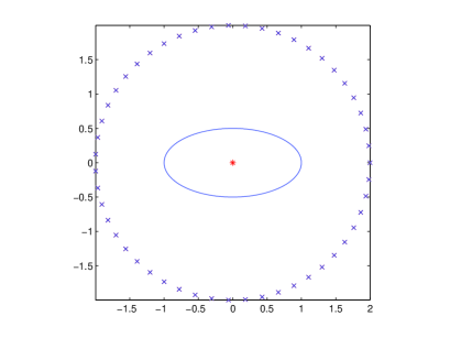
Figure 1: An example of the configuration for MSR data simulation. The unknown shape is an ellipse whose long and short axes are 2 and 1, respectively. $N=51$ sources/receivers (marked by “x”) are equally placed on a circle of radius $R=2$ centered at $z_{0}=[0,0]$ (marked by “*”).

6.1 Reconstruction of CGPTs

The theoretical analysis presented in section 3 suggests the following two step method for the reconstruction of CGPTs. First we apply (3.4) (or equivalently solve the least squares problem (3.2)) by fixing the truncation order $K$ as in (3.6):

$$K\leq\min\left(\frac{\log(\sigma_{\mathrm{noise}}/N)}{\log\varepsilon}-2,N/2\right).$$ (6.1)

Here, $\sigma_{\mathrm{noise}}$ is the standard deviation of the measurement noise and $\varepsilon=\delta/R$ with $\delta$ being the characteristic size of the target and $R$ the distance between the target center and the circular array of transmitters/receivers. Then, we keep only the first $m_{0}$ orders in the reconstructed CGPTs, with $m_{0}$ being the resolving order deduced from estimation (3.9):

$$m_{0}=\frac{\log\sigma_{\mathrm{noise}}-\log\tau_{0}}{2\log\varepsilon},$$ (6.2)

and $\tau_{0}\leq 1$ is the tolerance number introduced in (3.7). In all our numerical experiments we set the noise level $\sigma_{\mathrm{noise}}$ to:

$$\sigma_{\mathrm{noise}}=(\mathbf{V}_{\mbox{max}}-\mathbf{V}_{\mbox{min}})\sigma_{0},$$ (6.3)

with a positive constant $\sigma_{0}$ and $\mathbf{V}_{\mbox{max}}$ and $\mathbf{V}_{\mbox{min}}$ being the maximal and the minimal coefficient in the MSR matrix $\mathbf{V}$. Using the configuration given in Figure 1 and for various noise level, we reconstruct the CGPTs of the ellipse up to a truncation order $K$ which is determined as in (6.1). For each $k\leq K$, the relative error of the first $k$-th order reconstructed CGPTs is evaluated by comparing with their theoretical value ([7, Proposition 4.7]). The results are shown in Figure 2. In Figure 3 we plot the resolving order $m_{0}$ given by (6.2) and the relative error of the reconstruction within this order, for $\sigma_{0}$ in the range $[10^{-3},1]$.

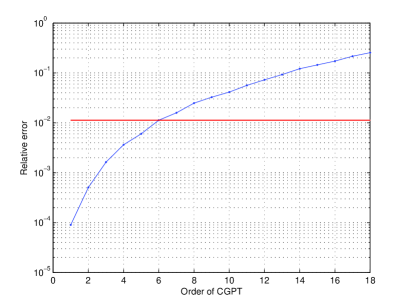
(a) $\sigma_{0}=0.01,m_{0}=6$

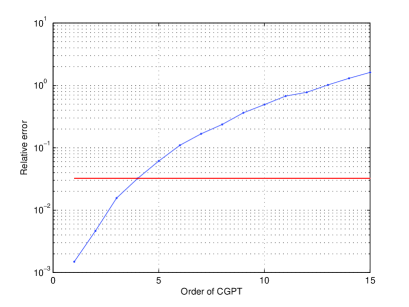
(b) $\sigma_{0}=0.1,m_{0}=4$

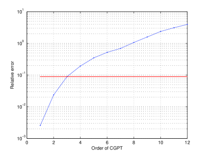
(c) $\sigma_{0}=0.5,m_{0}=3$

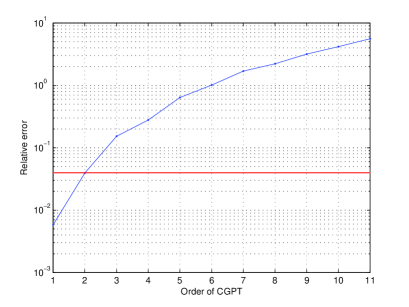
(d) $\sigma_{0}=1.0,m_{0}=2$

Figure 2: Relative error of the reconstructed CGPTs. For each noise level, we repeat the experiment 100 times (corresponding to 100 realizations of the noise) and the reconstruction is taken as their mean value. The horizontal solid line in each figure indicates the resolving order $m_{0}$ given by (6.2) with the tolerance number $\tau_{0}=10^{-1}$.

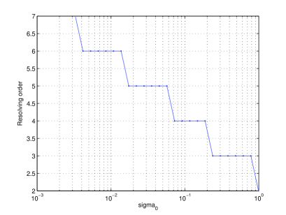
(a) Resolving order

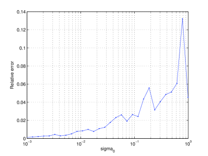
(b) Relative error

Figure 3: The resolving order $m_{0}$, for $\sigma_{0}\in[10^{-3},1],\tau_{0}=10^{-1},$ and the relative error of the reconstruction within this order. As in Figure 2, we repeat the experiment 100 times and the reconstruction is taken as their mean value. The large variations of the relative error in (b) for $\sigma_{0}>10^{-1}$ indicate the instability of the reconstruction for very noisy data.

6.2 Dictionary matching

We are now ready to present the results of the dictionary matching algorithms discussed in the sections 5.1 and 5.2. Unless specified, in the following we suppose that the unknown shape of the target $D_{0}$ is an exact copy of some element from the dictionary, up to a rigid transform and dilatation. As examples, we consider a dictionary of flowers and a dictionary of Roman letters. The aim is to identify the target $D_{0}$ from imaging data if it belongs to one of the dictionaries.

6.2.1 Matching on a dictionary of flowers

We start by considering a simple dictionary of rotation invariant “flowers”, on which the shape identification algorithm can be greatly simplified. The boundary of the $p$-th flower $B_{p}$ is defined as a small perturbation of the standard disk:

$$\partial B_{p}(\xi)=x(\xi)(1+\eta\cos(p\xi)),\mbox{ }x(\xi)=\begin{pmatrix}\cos\xi\\ \sin\xi\end{pmatrix},$$ (6.4)

where $p\geq 2$ is the number of petals and $\eta>0$ is a small constant. According to Proposition 4.3, $\mathbf{N}^{(1)}_{mn}(B_{p})$ is zero if $p$ does not divide $m+n$. For an unknown shape $D=T_{z}sR_{\theta}B_{p}$, the translation parameter is given by $z=\frac{\mathbf{N}^{(2)}_{12}(D)}{2\mathbf{N}^{(2)}_{11}(D)}$. Moreover, simple calculations show that $\mathcal{I}^{(1)}(D)$ and $\mathbf{N}^{(1)}(B_{p})$ have exactly the same zero patterns.

Therefore, we can find the true number of petals by searching the first nonzero anti-diagonal entry in $\mathcal{I}^{(1)}(D)$.

We fix $\eta=0.3$ (the amplitude of the perturbation introduced in (6.4)) and $\delta/R=0.5$. The unknown shape $D_{0}$ is obtained by applying the transform parameters $z=[16.3,-46.7],s=7.5,\theta=2.69$ on $B_{p}$, and the reference point for data acquisition is $z_{0}=[15,-45.5]$. The results for two flowers of 5 and 7 petals are shown in Figure 4, where we plot the mean absolute value of the anti-diagonal entries $mn$, for $m+n=l,l=2,\ldots,11,$ in $\mathcal{I}^{(1)}(D)$ by varying the noise level $\sigma_{0}$. One can clearly distinguish the peak which indicates the true number of petals for $\sigma_{0}$ up to $10^{-2}$.

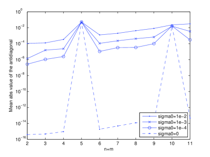
(a) $p=5$

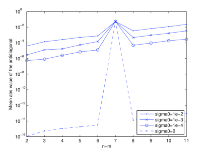
(b) $p=7$

Figure 4: Mean values of the anti-diagonal entries of $\mathcal{I}^{(1)}$ for the flowers of 5 and 7 petals at different noise levels.

Stability.

Let us consider now the model (6.4) with a general $\mathcal{C}^{1}$ function $h(\xi)$ in place of $\cos(p\xi)$. It was proven in [4] that:

$$\mathbf{N}^{(1)}_{mn}(B_{p})=2\pi\eta\frac{mn}{\lambda^{2}}\hat{h}_{m+n}+O(\eta^{2}).$$ (6.5)

Therefore as long as the perturbation $h(\xi)$ is close to $\cos(p\xi)$, the significant nonzero coefficients in $\mathcal{I}^{(1)}(D)$ will concentrate on the same anti-diagonals. We confirm this observation by applying the same procedure above on a flower with one damaged petal:

$$\partial B_{p}(\xi)=\begin{cases}x(\xi)f(\xi,t)\ &\mbox{ for }\xi\in[0,2\pi/p),\\ \vskip 6.0pt plus 2.0pt minus 2.0pt\cr x(\xi)(1+\eta\cos(p\xi))\ &\mbox{ for }\xi\in[2\pi/p,2\pi).\end{cases}$$ (6.6)

Here, $f(\cdot,t):\mathbb{R}\mapsto\mathbb{R}$ is a polynomial of order 6, constructed such that $\partial B_{p}$ is $\mathcal{C}^{2}$-smooth, and $t\in(0,1)$ is the percentage of the damage; see Figure 5. In Figure 6 we plot the mean value of the anti-diagonal entries at different noise levels. Compared to Figure 4, we see that the effect of the damage in the petal dominates the measurement noise. Nonetheless, the peak indicating the true number of petals is still visible.

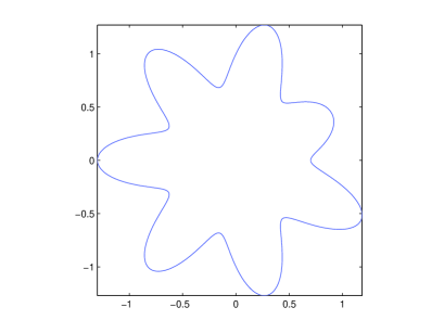
(a) $\tau_{0}=0.5$

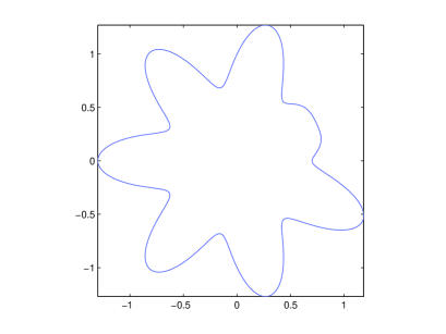
(b) $\tau_{0}=0.8$

Figure 5: Flowers with one damaged petal. The following parameters are used in (6.6): $p=7$, $\eta=0.3$, $t=0.5$ for (a) and $t=0.8$ for (b).

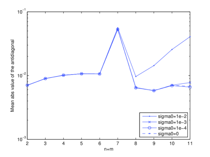
(a) $\tau_{0}=0.5$

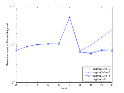
(b) $\tau_{0}=0.8$

Figure 6: Mean value of the anti-diagonal entries of $\mathcal{I}^{(1)}$ for the flowers of Figure 5 at different noise levels. The peaks indicate the number of petals.

6.2.2 Dictionary of letters

Next we consider here a dictionary consisting of 26 Roman capital letters without rotational symmetry. The shapes are defined in such a way that the holes inside the letters are filled, see Figure 11. We set $\delta/R=0.5$, $s=2.4762,\theta=6.0827,z=[33.3505,73.8395]$ and the center of mass of the target at $[33.4042,73.8627]$.

Performance of Algorithm 1.

First we test Algorithm 1 on the letter “P”. For the noiseless case ($\sigma_{0}=0$), the values of $e_{n}$ defined in Algorithm 1 are plotted in Figure 7 (a) and (b). These results suggest that the high order CGPTs can better distinguish similar shapes such as “P” and “R”, since they contain more high frequency information [4]. Nonetheless, the advantage of using high order CGPTs drops quickly when the data are contaminated by noise, and low order CGPTs provide more stable results in this situation, see Figure 7 (c) and (d).

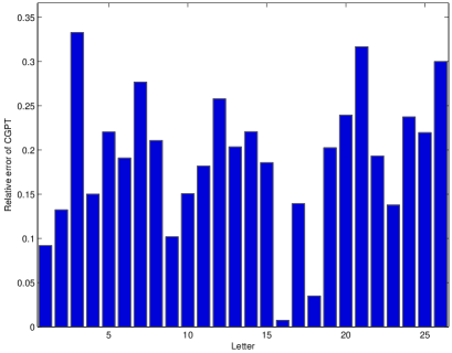
(a) $\sigma_{0}=0$, order $\leq 2$

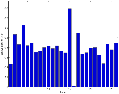
(b) $\sigma_{0}=0$, order $\leq 5$

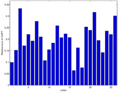
(c) $\sigma_{0}=0.1$, order $\leq 2$

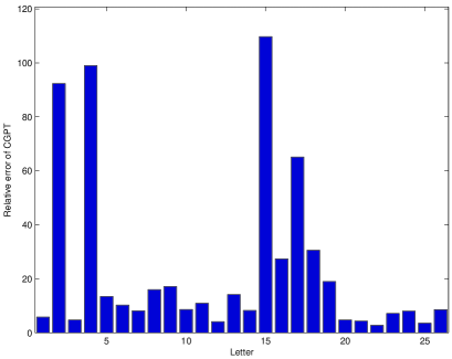
(d) $\sigma_{0}=0.1$, order $\leq 5$

Figure 7: The identification of the letter “P” using the first 2, and 5 orders CGPTs at noise levels $\sigma_{0}=0$ and $\sigma_{0}=0.1$. The bar represents the relative error $e_{n}$ between the CGPTs of the $n$-th letter and that of the data, as defined in Algorithm 1, and the shortest one in each figure corresponds to the identified letter. For (c) and (d), the experiment has been repeated for 100 times, using independent draws of white noise, and the results are the mean values of all experiments.

By repeating the same procedure as above, we apply Algorithm 1 on all letters at noise levels $\sigma_{0}=0$ and $\sigma_{0}=0.1$, and show the result in Figure 8 (a) and (c). At the coordinate $(m,n)$, the unknown shape is the $m$-th letter and the color represents the relative error (in logarithmic scale) of the CGPTs when compared with the $n$-th standard letter of the dictionary.

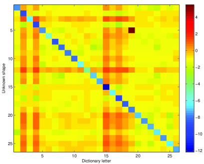
(a) $\sigma_{0}=0$, order $\leq 5$, Standard letters

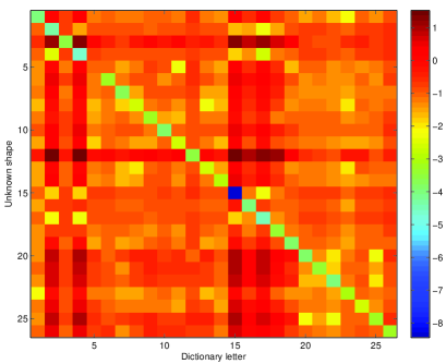
(b) $\sigma_{0}=0$, order $\leq 5$, Perturbed letters

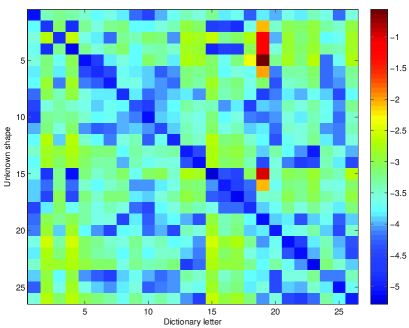
(c) $\sigma_{0}=0.1$, order $=1$, Standard letters

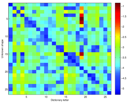
(d) $\sigma_{0}=0.1$, order $=1$, Perturbed letters

Figure 8: Algorithm 1 applied on the all 26 letters using the standard dictionary (Figure 11) at noise level $\sigma_{0}=0$ (first column) and $\sigma_{0}=0.1$ (second column), with the color indicating the relative error $e_{n}$ in logarithmic scale. The unknown shapes in the first row are exact copies of the standard dictionary, and in the second row are those of Figure 12. In (a) all letters are correctly identified, while in (b) letters ’E’ is identified as ’H’. For the noisy case, the experiment has been repeated 100 times, using independent draws of white noise, and the results in (c) and (d) are the mean values of all experiments, where only the first order CGPT is taken into account. 22 and 21 letters are correctly identified in (c) and (d), respectively.

Stability.

In real world applications we would like to have Algorithm 1 work also on letters which are not exact copies of the dictionary, such as handwriting letters. Figure 12 shows the letters obtained by perturbing and smoothing the dictionary elements. With these letters as unknown shapes, we repeat the experiment of Figure 8 (a) and (c) by applying Algorithm 1 on the standard dictionary and show the results in Figure 8 (b) and (d). Comparing with the results of Figure 8 (a) and (c), we see that Algorithm 1 remains quite stable, despite of some slight degradations.

Performance of Algorithm 2.

In the case of noiseless data, Algorithm 2 provides correct results with low computational cost. Here we repeat the experiment in Figure 7 (a) and (c) using Algorithm 2, and plot the error $e_{n}$ defined in Algorithm 2 in Figure 9. Nonetheless, when data are noisy, Algorithm 1 performs significantly better than Algorithm 2, as shown by Figure 10 where we compare the two algorithms for identifying letter “P” at various noise levels. Thanks to the debiasing step (5.11), Algorithm 1 is much more robust with respect to noise than Algorithm 2, in which there is no debiasing and the invariance of the shape descriptors $\mathcal{I}^{(1)}$ and $\mathcal{I}^{(2)}$ may be severely affected by noise (see Figure 10).

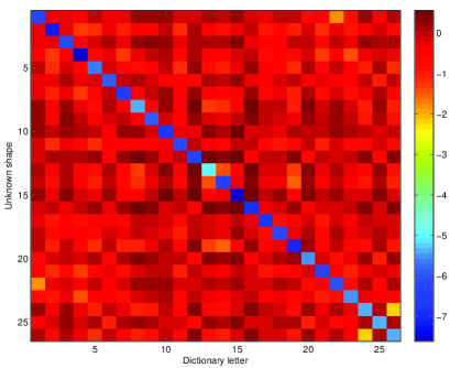
(a) $\sigma_{0}=0$, order $\leq 5$, Standard letters

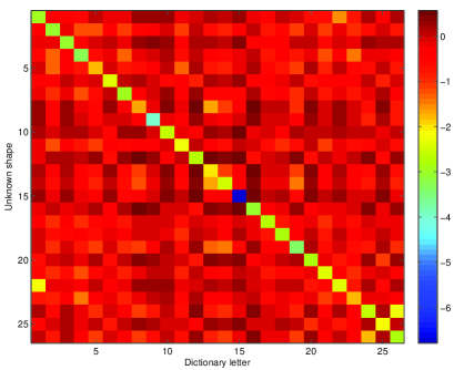
(b) $\sigma_{0}=0$, order $\leq 5$, Perturbed letters

Figure 9: Algorithm 2 applied on the all 26 letters using the standard dictionary (Figure 11) at noise level $\sigma_{0}=0$. The unknown shapes in (a) are exact copies of the standard dictionary, while in (b) are those of Figure 12. The color indicates the error $e_{n}$ in logarithmic scale. All letters are correctly identified in both (a) and (b).

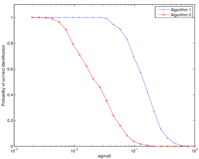
(a) order $\leq 2$

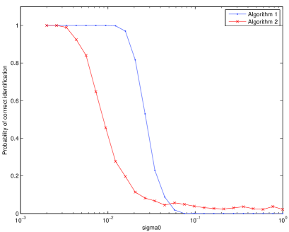
(b) order $\leq 3$

Figure 10: Comparison of Algorithm 2 and Algorithm 1 on identification of the standard letter “P”. At each noise level, the experiment has been repeated 1000 times, using independent draws of white noise. For each algorithm, the curve represents the percentage of experiments where the letter “P” is correctly identified.

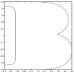
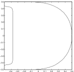
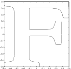
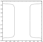
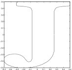
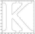
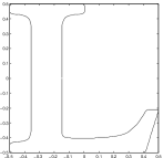
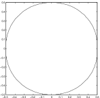
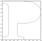
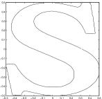
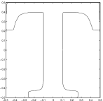
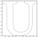
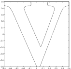
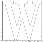
Figure 11: Dictionary of standard letters.

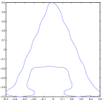
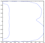
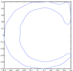
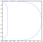
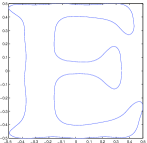
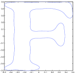
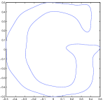
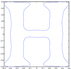
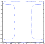
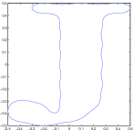
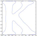
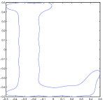
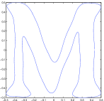
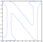
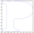
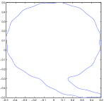
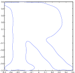
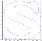
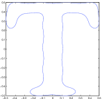
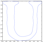
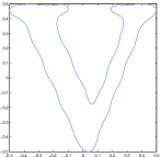
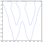
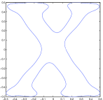
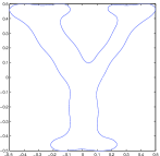
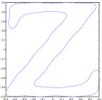
Figure 12: Non standard letters obtained by perturbing and smoothing those in Figure 11.

7 Conclusion

In this paper, we have designed two fast algorithms which identify a target using a dictionary of precomputed GPTs data. The target GPTs are computed from multistatic measurements by solving a linear system. The first algorithm matches the computed GPTs to precomputed ones (the dictionary elements) by finding rotation, scaling, and translation parameters and therefore, identifies the true target shape. The second algorithm is based on new invariants for the CGPTs. We have provided new shape descriptors which are invariant under translation, rotation, and scaling. The stability (in the presence of additive noise in multistatic measurements) and the resolution issues for both algorithms have been numerically investigated. The second algorithm is computationally much cheaper than the first one. However, it is more sensitive to measurement noise in the imaging data. To the best of our knowledge, our procedure is the first approach for real-time target identification in imaging using dictionary matching. It shows that GPT-based representations are an appropriate and natural tool for imaging. Our approach can be extended to electromagnetic and elastic imaging as well [12, 5]. We also to plan to use it for target tracking from imaging data.

Appendix A Appendix: Several Technical Estimates

A.1 The truncation error in the MSR expansion

Recall the expansion of the element in the MSR matrix (2.11). We prove the following estimate of the truncation error.

Proposition A.1.

Let $E_{rs}$ be as in (2.11). Set $\varepsilon=\delta/R$, the ratio between the typical length scale of the inclusion $D$ and the distance of the receivers (sources) from the inclusion. Assume also that $\varepsilon$ is much smaller than one. Then

$$|E_{rs}|\lesssim\varepsilon^{K+2}.$$ (A.1)

Proof. From the Taylor expansion of multivariate functions ([24], Chapter 1), we verify that the truncation error $E_{rs}$ can be written as

$$\int_{\partial D}e_{K}(y;x_{r},z)(\lambda I-\mathcal{K}_{D}^{*})^{-1}\bigg{[}\frac{\partial\Gamma(\cdot-x_{s})}{\partial\nu}\bigg{]} (y)ds(y)$$

$$+\int_{\partial D}\Gamma_{K}(y;x_{r},z) (\lambda I-\mathcal{K}_{D}^{*})^{-1}\bigg{[}\frac{\partial}{\partial\nu}e_{K}(\cdot;z,x_{s})\bigg{]}(y)ds(y).$$

Here, $\Gamma_{K}(y;x_{r},z)$ and $e_{K}(y;x_{r},z)$ (and similarly $e_{K}(y;z,x_{s})$) are given by

$$\Gamma_{K}(y;x_{r},z) =\sum_{k=1}^{K}\sum_{|\alpha|=k}\frac{(-1)^{|\alpha|}}{\alpha!}\partial^{\alpha}\Gamma(x_{r}-z)(y-z)^{\alpha},$$

$$e_{K}(y;x_{r},z) =\sum_{|\alpha|=K+1}\Big{(}\frac{1}{\alpha!}\int_{0}^{1}(1-s)^{K}\partial^{\alpha}\Gamma(x_{r}-z-s(y-z))ds\Big{)}(y-z)^{\alpha}.$$

Due to the invariance relation (4.7), the operator $(\lambda I-\mathcal{K}_{D}^{*})^{-1}$, as an operator from the space $L^{2}(\partial D)$ to itself, is bounded uniformly with respect to the scaling of $D$. Consequently, the first term in $E_{rs}$ is bounded by

$$C\|e_{K}(\cdot;x_{r},z)\|_{L^{\infty}(\partial D)}\|\frac{\partial\Gamma(\cdot-x_{s})}{\partial\nu}\|_{L^{2}(\partial D)}|\partial D|^{\frac{1}{2}}\leq C\|e_{K}\|_{L^{\infty}(\partial D)}\|\frac{\partial\Gamma(\cdot-x_{s})}{\partial\nu}\|_{L^{\infty}(\partial D)}|\partial D|.$$

Assume that $z\in D$; the distance between $\overline{D}$ and the receivers (sources) is of order $R$. From the above expression of $e_{K}$, the explicit form of $\partial^{\alpha}\Gamma$ in (2.18), and the fact that $|y-z|\leq C\delta$ for $y\in\overline{D}$, we have

$$|e_{K}(y;x_{r},z)|\leq C\left(\sum_{|\alpha|=K+1}\frac{1}{\alpha!}\|\partial^{\alpha}\Gamma_{r}(x_{r}-\cdot)\|_{\mathcal{C}(\overline{D})}\right)|y-z|^{K+1}\leq C\left(\frac{\delta}{R}\right)^{K+1}.$$

Similarly, we have $\|\partial_{\nu}\Gamma(\cdot-x_{s})\|_{L^{\infty}(\partial D)}\leq CR^{-1}$. The measure $|\partial D|$ in dimension two is of order $\delta$. Substituting these estimates into the bound for the first term in $E_{rs}$, we see that it is bounded by $C\varepsilon^{K+2}$.

The second term can be bounded from above by

$$C\|\Gamma_{K}\|_{L^{\infty}(\partial D)}\|\frac{\partial e_{K}(\cdot;z,x_{s})}{\partial\nu}\|_{L^{\infty}(\partial D)}|\partial D|.$$

We have $\|\Gamma_{K}(\cdot;x_{r},z)\|_{L^{\infty}(\partial D)}\leq C\varepsilon$, which is the order of the leading term. Further, from the explicit form of $e_{K}$, we verify that

$$\|\frac{\partial e_{K}(\cdot;z,x_{s})}{\partial\nu}\|_{L^{\infty}(\partial D)}\leq C\left(\|\Gamma(\cdot-x_{s})\|_{\mathcal{C}^{K+2}(\overline{D})}\delta^{K+1}+\|\Gamma(\cdot-x_{s})\|_{\mathcal{C}^{K+1}(\overline{D})}\delta^{K}\right)\leq C\frac{\delta^{K}}{R^{K+1}}.$$

As a result, the above upper bound for the second term in $E_{rs}$ is of order $\varepsilon^{K+2}$ as well. This proves (A.1). $\Box$

Proposition A.2.

The solution $u_{s}(x)$ defined by the transmission problem (2.2) satisfies the symmetry property

$$u_{s}(x_{r})=u_{r}(x_{s}).$$ (A.2)

Proof. Let $\Omega^{\varepsilon}_{s}$ be the the ball of radius $\varepsilon$ centered at $x_{s}$, and $\Omega^{\varepsilon}_{r}$ the ball of radius $\varepsilon$ centered at $x_{r}$. Let $\Omega_{\varepsilon}$ be the domain $B_{R}\backslash(\Omega^{\varepsilon}_{r}\cup\Omega^{\varepsilon}_{s}\cup D)$ where $B_{R}$ is a sufficiently large ball with radius $R$. Then we have

$$0 =\int_{\Omega_{\varepsilon}}\bigg{(}u_{s}(x)\Delta u_{r}(x)-u_{r}(x)\Delta u_{s}(x)\bigg{)}dx=\int_{\partial\Omega_{\varepsilon}}\bigg{(}u_{s}(x)\frac{\partial u_{r}}{\partial n}(x)-u_{r}(x)\frac{\partial u_{s}}{\partial n}(x)\bigg{)}ds(x)$$

$$=-\int_{\partial\Omega^{\varepsilon}_{s}}\bigg{(}u_{s}(x)\frac{\partial u_{r}}{\partial n}(x)-u_{r}(x)\frac{\partial u_{s}}{\partial n}(x)\bigg{)}ds(x)-\int_{\partial\Omega^{\varepsilon}_{r}}\bigg{(}u_{s}(x)\frac{\partial u_{r}}{\partial n}(x)-u_{r}(x)\frac{\partial u_{s}}{\partial n}(x)\bigg{)}ds(x)$$

$$\quad-\int_{\partial D}\bigg{(}u_{s}(x)\frac{\partial u_{r}}{\partial n}(x)\Big{|}_{+}-u_{r}(x)\frac{\partial u_{s}}{\partial n}(x)\Big{|}_{+}\bigg{)}ds(x)+\int_{\partial B_{R}}\bigg{(}u_{s}(x)\frac{\partial u_{r}}{\partial n}(x)\Big{|}_{+}-u_{r}(x)\frac{\partial u_{s}}{\partial n}(x)\Big{|}_{+}\bigg{)}ds(x)$$

$$=J^{\varepsilon}_{s}+J^{\varepsilon}_{r}+J_{D}+J_{R}.$$

For $J_{D}$, thanks to the jump conditions in (2.2), we have that

$$J_{D}=\kappa\int_{\partial D}\bigg{(}u_{r}(x)\frac{\partial u_{s}}{\partial n}(x)\Big{|}_{-}-u_{s}(x)\frac{\partial u_{r}}{\partial n}(x)\Big{|}_{-}\bigg{)}ds(x)=\kappa\int_{D}\bigg{(}u_{r}(x)\Delta u_{s}(x)-u_{s}(x)\Delta u_{r}(x)\bigg{)}dx=0.$$

The other two terms $J^{\varepsilon}_{s}$ and $J^{\varepsilon}_{r}$ can be treated similarly; hence we focus on the first item. We’ve shown that $u_{s}(x)=\Gamma(x-x_{s})+\mathcal{S}_{D}[\phi_{s}]$. In a neighborhood of $\Omega^{\varepsilon}_{s}$, we have

$$\|u_{r}\|_{L^{\infty}}+\|\nabla u_{r}\|_{L^{\infty}}+\|\mathcal{S}_{D}[\phi_{s}]\|_{L^{\infty}}+\|\nabla\mathcal{S}_{D}[\phi_{s}]\|_{L^{\infty}}\leq C.$$

Consequently,

$$\left|\int_{\partial\Omega^{\varepsilon}_{s}}u_{s}(x)\frac{\partial u_{r}}{\partial n}(x)\right|\leq C\int_{\partial B_{\varepsilon}(x_{s})}(1+|\log\varepsilon|)ds(x)\leq C\varepsilon|\log\varepsilon|.$$

$$\left|\int_{\partial\Omega^{\varepsilon}_{s}}u_{r}(x)\left(\frac{\partial u_{s}}{\partial n}(x)-\frac{\partial\Gamma}{\partial n}(x-x_{s})\right)\right|ds(x)\leq\left|\int_{\partial\Omega^{\varepsilon}_{s}}u_{r}(x)\frac{\partial\mathcal{S}_{D}[\phi_{s}]}{\partial n}(x)ds(x)\right|\leq C\varepsilon.$$

These estimates imply that

$$\lim_{\varepsilon\to 0}J^{\varepsilon}_{s}=\lim_{\varepsilon\to 0}\int_{\partial B_{\varepsilon}(x_{s})}u_{r}(x_{s}+y)\frac{\partial\Gamma}{\partial n}(y)ds(y)=\lim_{\varepsilon\to 0}\frac{1}{2\pi\varepsilon}\int_{0}^{2\pi}\varepsilon u_{r}(x_{s}+\varepsilon\theta)d\theta=u_{r}(x_{s}).$$

The same analysis applied to $J^{\varepsilon}_{r}$ shows that $\lim_{\varepsilon\to 0}J^{\varepsilon}_{r}=-u_{s}(x_{r})$.

To control $J_{R}$, we recall the fact that $\mathcal{S}_{D}[\phi]$ decays as $|x|^{-1}$ and $\nabla\mathcal{S}_{D}[\phi]$ decays as $|x|^{-2}$ for $\phi\in L^{2}(\partial D)$ satisfying $\int_{\partial D}\phi ds=0$; these estimates imply that the logarithmic part of $u_{s}$ dominates. Therefore,

$$\lim_{R\to\infty}J_{R}=\lim_{R\to\infty}\int_{\partial B_{R}}\log|x-x_{s}|\frac{\langle\nu_{x},x-x_{r}\rangle}{|x-x_{r}|^{2}}-\log|x-x_{r}|\frac{\langle\nu_{x},x-x_{s}\rangle}{|x-x_{s}|^{2}}ds(x).$$

The integrand above can be written as

$$\left(\log\frac{|x-x_{s}|}{|x-x_{r}|}\right)\frac{\langle\nu_{x},x-x_{r}\rangle}{|x-x_{r}|^{2}}+\log|x-x_{r}|\left[\frac{\langle\nu_{x},x-x_{r}\rangle}{|x-x_{r}|^{2}}-\frac{\langle\nu_{x},x-x_{s}\rangle}{|x-x_{s}|^{2}}\right].$$

We verify that the first term is of order $o(\frac{1}{R})$; its contribution to the limiting integral is hence negligible. The second term in the integrand can be further written as

$$\log|x-x_{r}|\left[\langle\nu_{x},x-x_{r}\rangle\left(\frac{1}{|x-x_{r}|^{2}}-\frac{1}{|x-x_{s}|^{2}}\right)+\frac{\langle\nu_{x},x-x_{r}-(x-x_{s})\rangle}{|x-x_{s}|^{2}}\right].$$

From

$$\frac{1}{|x-x_{r}|^{2}}-\frac{1}{|x-x_{s}|^{2}}=\frac{|x_{s}|^{2}-|x_{r}|^{2}+2\langle x,x_{r}-x_{s}\rangle}{|x-x_{r}|^{2}|x-x_{s}|^{2}},$$

we verify that the second term in the integrand is of order $O(\log R/R^{2})$; hence its contribution to the limiting integral is also zero. To summarize, we have $\lim_{R\to\infty}J_{R}=0$.

From the above analysis, we take the limit $\varepsilon\to 0,R\to\infty$ on the equality $0=J^{\varepsilon}_{s}+J^{\varepsilon}_{r}+J_{D}+J_{R}$ and conclude that (A.2) holds. $\Box$

A.2 Proof of formula (2.18)

Formula (2.18) is well-known. We include a proof for reader’s sake.

In order to prove (2.18), we need to find the derivative of the function $\log|x|$. To this end, we consider the Taylor expansion of the logarithmic function around the point $x$. The most convenient method for this expansion is to view the space variables as complex numbers. For a small perturbation $z$ of the point $x$ ($x,z\in\mathbb{C}$), we calculate

$$\log|x-z|-\log|x|=\frac{1}{2}\left([\log(x-z)-\log x]+[\log(\overline{x}-\overline{z})-\log\overline{x}]\right).$$

To expand the first item on the right-hand side of the above equality, we write it as $\log(1-\frac{z}{x})$, and since $|\frac{z}{x}|<1$ we obtain the expansion

$$\log(1-\frac{z}{x})=-\sum_{j=1}^{\infty}\frac{1}{j}\left(\frac{z}{x}\right)^{j}=-\sum_{j=1}^{\infty}\frac{1}{j}\left(\frac{r_{z}e^{i\theta_{z}}}{r_{x}e^{i\theta_{x}}}\right)^{j}.$$

Taking the conjugate, we obtain the expansion for $\log(\overline{x}-\overline{z})-\log\overline{x}$. Consequently, we have

$$\log|x-z|-\log|x| =-\frac{1}{2}\sum_{j=1}^{\infty}\frac{1}{j}\left[\left(\frac{r_{z}e^{i\theta_{z}}}{r_{x}e^{i\theta_{x}}}\right)^{j}+\left(\frac{r_{z}e^{-i\theta_{z}}}{r_{x}e^{-i\theta_{x}}}\right)^{j}\right]$$

$$=-\sum_{j=1}^{\infty}\frac{1}{j}\left(\frac{\cos j\theta_{x}}{r_{x}^{j}}[r_{z}^{j}\cos j\theta_{z}]+\frac{\sin j\theta_{x}}{r_{x}^{j}}[r_{z}^{j}\sin j\theta_{z}]\right)$$

$$=-\sum_{j=1}^{\infty}\frac{1}{j}\left(\frac{\cos j\theta_{x}}{r_{x}^{j}}\sum_{|\alpha|=j}a^{j}_{\alpha}z^{\alpha}+\frac{\sin j\theta_{x}}{r_{x}^{j}}\sum_{|\alpha|=j}b^{j}_{\alpha}z^{\alpha}\right).$$

In the last equality, we understood the variable $z$ as real variable and used the representation (2.13). Compare the last term of the above formula with the (real-variable) multivariate expansion of $\log|x-z|-\log|x|$, we observe that

$$\sum_{|\alpha|=j}\frac{(-1)^{j}}{\alpha!}(\partial^{\alpha}_{x}\log|x|)z^{\alpha}=-\sum_{|\alpha|=j}\frac{1}{j}\left(\frac{\cos j\theta_{x}}{r_{x}^{j}}a^{j}_{\alpha}+\frac{\sin j\theta_{x}}{r_{x}^{j}}b^{j}_{\alpha}\right)z^{\alpha}.$$

For each double index $\alpha$, we get (2.18).

A.3 Proof of formula (3.3)

The proof is a straightforward computation. The elements of the matrix $\mathbf{C}^{t}\mathbf{C}$ correspond to inner products of columns of the matrix $\mathbf{C}$, that is, the inner products of vectors formed by evaluating $\sin$ and $\cos$ functions at $(k_{1}\theta_{1},\ldots,k_{1}\theta_{N})$ and at $(k_{2}\theta_{1},\ldots,k_{2}\theta_{N})$, where $k_{1},k_{2}=1,2,\ldots,K$, $k_{1}+k_{2}\leq 2K<N$, and $\theta_{j}=2\pi j/N$, $j=1,2,\ldots,N$. When two $\cos$ vectors are chosen, the inner product becomes

$$\sum_{j=1}^{N}\cos k_{1}\theta_{j}\cos k_{2}\theta_{j}=\frac{1}{4}\sum_{j=1}^{N}\left(e^{i\frac{2\pi(k_{1}+k_{2})j}{N}}+e^{-i\frac{2\pi(k_{1}+k_{2})j}{N}}+e^{i\frac{2\pi(k_{1}-k_{2})j}{N}}+e^{-i\frac{2\pi(k_{1}-k_{2})j}{N}}\right).$$

Since $k_{1}+k_{2}$ is an integer less than $N$, the first two sums always vanish because

$$\sum_{j=1}^{N}e^{i\frac{2\pi(k_{1}+k_{2})j}{N}}=\frac{1-e^{i2\pi(k_{1}+k_{2})}}{1-e^{i\frac{2\pi(k_{1}+k_{2})}{N}}}=0.$$

When $k_{1}=k_{2}$, the last two sums contribute and the overall result is $N/2$. When $k_{1}\neq k_{2}$, the inner products under estimation is zero according to the above observation.

The case of inner product with $\sin$ and $\sin$ or $\cos$ and $\cos$ vectors can be similarly analyzed, and it can be easily seen that (3.3) holds.

References

- [1] H. Ammari, P. Garapon, F. Jouve, H. Kang, M. Lim, and S. Yu, A new optimal control approach for the reconstruction of extended inclusions, SIAM J. Control Opt., to appear.
- [2] H. Ammari, J. Garnier, and V. Jugnon, Detection, reconstruction, and characterization algorithms from noisy data in multistatic wave imaging, submitted, (2011).
- [3] H. Ammari, J. Garnier, H. Kang, M. Lim, and K. Sølna, Multistatic imaging of extended targets, SIAM J. Imaging Sci., to appear.
- [4] H. Ammari, J. Garnier, H. Kang, M. Lim, and S. Yu, Generalized polarization tensors for shape description, submitted, (2011).
- [5] H. Ammari, J. Garnier, and K. Sølna, Resolution and stability analysis in full-aperature, linearized conductivity and wave imaging, Proc. Amer. Math. Soc., to appear.
- [6] H. Ammari and H. Kang, Reconstruction of small inhomogeneities from boundary measurements, vol. 1846, Lecture Notes in Mathematics, Springer-Verlag, Berlin, 2004.
- [7] H. Ammari and H. Kang, Polarization and moment tensors: with applications to inverse problems and effective medium theory, vol. 162, Springer-Verlag, 2007.
- [8] H. Ammari and H. Kang, High-order terms in the asymptotic expansions of the steady-state voltage potentials in the presence of conductivity inhomogeneities of small diameter, SIAM J. Math. Anal., 34 (2003), pp. 1152–1166.
- [9] H. Ammari and H. Kang, Properties of generalized polarization tensors, SIAM Multiscale Model. Simul., 1 (2003), pp. 335–348.
- [10] H. Ammari, H. Kang, H. Lee, and M. Lim, Enhancement of near cloaking using generalized polarization tensors vanishing structures. Part I: The conductivity problem, Comm. Math. Phys., to appear.
- [11] H. Ammari, H. Kang, M. Lim, and H. Zribi, The generalized polarization tensors for resolved imaging. Part I: Shape reconstruction of a conductivity inclusion, Math. Comp., 81 (2012), pp. 367–386.
- [12] H. Ammari, H. Kang, E. Kim, and J.-Y. Lee, The generalized polarization tensors for resolved imaging. Part II: Shape and electromagnetic parameters reconstruction of an electromagnetic inclusion from multistatic measurements, Math. Comp., 81 (2012), pp. 839–860.
- [13] H. Ammari, H. Kang, and K. Touibi, Boundary layer techniques for deriving the effective properties of composite materials, Asymp. Anal., 41 (2005), pp. 119–140.
- [14] M. Brühl, M. Hanke, and M. S. Vogelius, A direct impedance tomography algorithm for locating small inhomogeneities, Numer. Math., 93 (2003), pp. 635–654.
- [15] Y. Capdeboscq, A. B. Karrman, and J.-C. Nédélec, Numerical computation of approximate generalized polarization tensors, Appl. Anal., to appear.
- [16] D.J. Cedio-Fengya, S. Moskow, and M.S. Vogelius, Identification of conductivity imperfections of small diameter by boundary measurements: Continuous dependence and computational reconstruction, Inverse Problems, 14 (1998), pp. 553–595.
- [17] G. Dassios and R. Kleinman, Low frequency scattering, Oxford Mathematical Monographs, Oxford University Press, New York, 2000.
- [18] A. Friedman and M.S. Vogelius, Identification of small inhomogeneities of extreme conductivity by boundary measurements: a theorem on continuous dependence, Arch. Rat. Mech. Anal., 105 (1989), pp. 299–326.
- [19] E. Haber, U. M. Ascher, and D. Oldenburg, On optimization techniques for solving nonlinear inverse problems, Inverse Problems, 16 (2000), pp. 1263–1280.
- [20] C. L. Lawson and R. J. Hanson, Solving Least Squares Problems, vol. 15 of Classics in Applied Mathematics, Society for Industrial and Applied Mathematics (SIAM), Philadelphia, PA, 1995. Revised reprint of the 1974 original.
- [21] G. W. Milton, The Theory of Composites, Cambridge Monographs on Applied and Computational Mathematics, Cambridge University Press, 2001.
- [22] G. Pólya and G. Szegö, Isoperimetric Inequalities in Mathematical Physics, Annals of Mathematical Studies Number 27, Princeton University Press, Princeton, NJ, 1951.
- [23] A. Tarantola, Inverse Problem Theory and Methods for Model Parameter Estimation, SIAM, Philadelphia, PA, 2005.
- [24] M. E. Taylor, Partial differential equations. I, vol. 115 of Applied Mathematical Sciences, Springer-Verlag, New York, 1996. Basic theory.
- [25] C. R. Vogel, Computational Methods for Inverse Problems, Frontiers in Applied Mathematics, vol. 23, SIAM, Philadelphia, PA, 2002.