Markov degree of the three-state toric homogeneous Markov chain model

Abstract

We consider the three-state toric homogeneous Markov chain model (THMC) without loops and initial parameters. At time $T$, the size of the design matrix is $6\times 3\cdot 2^{T-1}$ and the convex hull of its columns is the model polytope. We study the behavior of this polytope for $T\geq 3$ and we show that it is defined by $24$ facets for all $T\geq 5$. Moreover, we give a complete description of these facets. From this, we deduce that the toric ideal associated with the design matrix is generated by binomials of degree at most $6$. Our proof is based on a result due to Sturmfels, who gave a bound on the degree of the generators of a toric ideal, provided the normality of the corresponding toric variety. In our setting, we established the normality of the toric variety associated to the THMC model by studying the geometric properties of the model polytope.

1 Introduction

A discrete time Markov chain, $X_{t}$ for $t=1,2,\ldots$, is a stochastic process with the Markov property, that is $P(X_{t+1}=y|X_{1}=x_{1},\ldots,X_{t-1}=x_{t-1},X_{t}=x)=P(X_{t+1}=y|X_{t}=x)$ for any states $x,\,y$. Discrete time Markov chains have applications in several fields, such as physics, chemistry, information sciences, economics, finances, mathematical biology, social sciences, and statistics stochastics . In this paper, we consider a discrete time Markov chain $X_{t}$ over a set of states $[S]=\{1,\ldots,S\}$, with $t=1,\ldots,T$ ($T\geq 3$), focusing on the case $S=3$.

Discrete time Markov chains are often used in statistical models to fit the observed data from a random physical process. Sometimes, in order to simplify the model, it is convenient to consider time-homogeneous Markov chains, where the transition probabilities do not depend on the time, in other words, when

$$P(X_{t+1}{=}y|X_{t}{=}x)=P(X_{2}{=}y|X_{1}{=}x)\quad\forall\,x,\,y\in[S]\text{ and for any }t=1\ldots,T{-}1.$$

Let ${\bf w}=s_{1}\cdots s_{T}$ denote a word of length $T$ on states $[S]$. Let $p({\bf w})$ denote the likelihood of observing the word ${\bf w}$. In the time-homogeneous Markov chain model, this likelihood is written as the product of probabilities

$$P({\bf w})=\pi_{s_{1}}p_{s_{1},s_{2}}\cdots p_{s_{T-1},s_{T}},$$ (1.1)

where, $\pi_{s_{i}}$ indicates the initial distribution at the first state, and $p_{s_{i},s_{j}}$ are the transition probabilities from state $s_{i}$ to $s_{j}$. In the usual time-homogeneous Markov chain model it is assumed that the row sums of the transition probabilities are equal to one: $\sum_{j=1}^{S}p_{i,j}=1$, $\forall i\in[S]$. In addition, the toric homogeneous Markov chain (THMC) model is also described by (1.1), but where the parameters $p_{i,j}$ are free and the row sums of the transition probabilities are not restricted.

In many cases the parameters $\pi_{s_{1}}$ for the initial distribution are known, or sometimes these parameters are all constant, namely $\pi_{1}=\pi_{2}=\cdots=\pi_{S}=c$; in this situation it is no longer necessary to take them in consideration in expression (1.1), making the model simpler. Another simplification that arises from practice is when the only transition probabilities considered are those between two different states, i.e. when $p_{i,j}=0$ whenever $i=j$; this situation is referred as the THMC model without self-loops. In this paper, we consider both simplifications of the THMC model.

In order for a statistical model to reflect the observed data, it has to pass a goodness-of-fit test. For instance, for the time-homogeneous Markov chain model, it is necessary to test if the assumption of time-homogeneity fits the observed data. In 1998, Diaconis-Sturmfels developed a Markov Chain Monte Carlo method (MCMC) for goodness-of-fit test by using Markov bases diaconis-sturmfels .

A Markov basis is a set of moves between objects with the same sufficient statistics so that the transition graph for the MCMC is guaranteed to be connected for any observed value of the sufficient statistics (see Section 2.1 and stochastics ). In algebraic terms, a Markov basis is a generating set of a toric ideal defined as the kernel of a monomial map between two polynomial rings. In algebraic statistics, the monomial map comes from the design matrix associated with a statistical model.

In Hara:2010vn , the authors provided a full description of the Markov bases for the THMC model in two states (i.e. when $S=2$) which does not depend on $T$, even though the toric ideal lies on a polynomial ring with $2^{T}$ indeterminates. Inspired by their work, we study the algebraic and polyhedral properties of the Markov bases of the three-state THMC model without initial parameters and without self-loops. We showed that for arbitrarily large time $T\geq 5$, the model polytope –the convex hull of the columns of the design matrix– has only $24$ facets and we provide a complete description of them. Moreover, by showing the normality of the polytope, we deduced that the Markov bases of the model consist of binomials of degree at most $6$.

The outline of this paper is as follows. In Section 2, we recall some definitions from Markov bases theory. In Section 3, we explicitly describe the hyperplane representation of the model polytope for the three-state THMC model without self-loops for any time $T\geq 5$. In Section 4, we show that the model polytope is normal for arbitrary $T\geq 3$, this is equivalent to show that the semigroup generated by the columns of the design matrix is integrally closed. Finally, using these results, we prove the bound on the degree of the Markov bases in Section 5; and we conclude that section with some observations based on the analysis of our computational experiments.

2 Notation

Let $\Omega_{S,T}$ be the set of all words of length $T$ on states $[S]$ such that every word has no self-loops; that is, if $\mathchoice{\mbox{\boldmath$\displaystyle\bf w$}}{\mbox{\boldmath$\textstyle\bf w$}}{\mbox{\boldmath$\scriptstyle\bf w$}}{\mbox{\boldmath$\scriptscriptstyle\bf w$}}=(s_{1},\ldots,s_{T})\in\Omega_{S,T}$ then $s_{i}\neq s_{i+1}$ for $i=1,\ldots,T{-}1$. We define ${\mathcal{P}^{*}}(\Omega_{S,T})$ to be the set of all multisets of words in $\Omega_{S,T}$.

Let ${\mathbb{V}}$ be the real vector space with basis $\Omega_{S,T}$ and note that ${\mathbb{V}}\cong{\mathbb{R}}^{S(S-1)^{T-1}}$. We recall some definitions from the book of Pachter and Sturmfels Pachter:2005kx . Let $A=(a_{ij})$ be a non-negative integer $d{\times}m$-matrix with the property that all column sums are equal:

$$\sum_{i=1}^{d}a_{i1}=\sum_{i=1}^{d}a_{i2}=\cdots=\sum_{i=1}^{d}a_{im}.$$

Write $A=[\mathchoice{\mbox{\boldmath$\displaystyle\bf a$}}{\mbox{\boldmath$\textstyle\bf a$}}{\mbox{\boldmath$\scriptstyle\bf a$}}{\mbox{\boldmath$\scriptscriptstyle\bf a$}}_{1}\;\mathchoice{\mbox{\boldmath$\displaystyle\bf a$}}{\mbox{\boldmath$\textstyle\bf a$}}{\mbox{\boldmath$\scriptstyle\bf a$}}{\mbox{\boldmath$\scriptscriptstyle\bf a$}}_{2}\;\cdots\;\mathchoice{\mbox{\boldmath$\displaystyle\bf a$}}{\mbox{\boldmath$\textstyle\bf a$}}{\mbox{\boldmath$\scriptstyle\bf a$}}{\mbox{\boldmath$\scriptscriptstyle\bf a$}}_{m}]$ where $\mathchoice{\mbox{\boldmath$\displaystyle\bf a$}}{\mbox{\boldmath$\textstyle\bf a$}}{\mbox{\boldmath$\scriptstyle\bf a$}}{\mbox{\boldmath$\scriptscriptstyle\bf a$}}_{j}$ are the column vectors of $A$ and define $\theta^{\mathchoice{\mbox{\boldmath$\displaystyle\bf a$}}{\mbox{\boldmath$\textstyle\bf a$}}{\mbox{\boldmath$\scriptstyle\bf a$}}{\mbox{\boldmath$\scriptscriptstyle\bf a$}}_{j}}=\prod_{i=1}^{d}\theta_{i}^{a_{ij}}$ for $j=1,\ldots,m$. The toric model of $A$ is the image of the orthant ${\mathbb{R}}^{d}_{\geq 0}$ under the map

$$f:{\mathbb{R}}^{d}\rightarrow{\mathbb{R}}^{m},\quad\theta\mapsto\frac{1}{\sum_{j=1}^{m}\theta^{\mathchoice{\mbox{\boldmath$\displaystyle\bf a$}}{\mbox{\boldmath$\textstyle\bf a$}}{\mbox{\boldmath$\scriptstyle\bf a$}}{\mbox{\boldmath$\scriptscriptstyle\bf a$}}_{j}}}\left(\theta^{\mathchoice{\mbox{\boldmath$\displaystyle\bf a$}}{\mbox{\boldmath$\textstyle\bf a$}}{\mbox{\boldmath$\scriptstyle\bf a$}}{\mbox{\boldmath$\scriptscriptstyle\bf a$}}_{1}},\ldots,\theta^{\mathchoice{\mbox{\boldmath$\displaystyle\bf a$}}{\mbox{\boldmath$\textstyle\bf a$}}{\mbox{\boldmath$\scriptstyle\bf a$}}{\mbox{\boldmath$\scriptscriptstyle\bf a$}}_{m}}\right).$$

Here we have $d$ parameters $\theta=(\theta_{1},\ldots,\theta_{d})$ and a discrete state space of size $m$. In our setting, the discrete space will be the set of all possible words on $[S]$ of length $T$ without self-loops ($\Omega_{S,T}$) and we can think of $\theta_{1},\ldots,\theta_{d}$ as the probabilities $p_{1,2},p_{1,3},\dots,p_{S-1,S}$.

In this paper, we focus on the THMC model without initial parameters and with no self-loops in three states, (i.e., $S=3$), which is parametrized by $6$ positive real variables: $p_{1,2},\,p_{1,3},\,p_{2,1},\,p_{2,3}$, $p_{3,1},\,p_{3,2}$. In this case, we only write $\Omega_{T}$ instead of $\Omega_{3,T}$. The number of parameters is $d=6$ and the size of the discrete space is $m=3\cdot 2^{T-1}$, which is precisely the number of words in $\Omega_{T}$. The model we study is thus the toric model represented by the $6\times 3\cdot 2^{T-1}$ matrix $A^{T}$, which will be referred to as the design matrix for the model on $3$ states with time $T$. The rows of $A^{T}$ are indexed by elements in $\Omega_{2}$ and the columns are indexed by words in $\Omega_{T}$. The entry of $A^{T}$ indexed by row $\sigma_{1}\sigma_{2}\in\Omega_{2}$, and column $\mathchoice{\mbox{\boldmath$\displaystyle\bf w$}}{\mbox{\boldmath$\textstyle\bf w$}}{\mbox{\boldmath$\scriptstyle\bf w$}}{\mbox{\boldmath$\scriptscriptstyle\bf w$}}=(s_{1},\ldots,s_{T})\in\Omega_{T}$ is equal to the cardinality of the set $\left\{\,i\in\{1,\ldots,T{-}1\}\mid\sigma_{1}\sigma_{2}=s_{i}s_{i+1}\,\right\}$.

Example 2.1

Ordering $\Omega_{2}$ and $\Omega_{T}$ lexicographically, and letting $T=4$, the matrix $A^{4}$ is:

	1212	1213	1231	1232	1312	1313	1321	1323	2121	2123	2131	2132	2312	2313	2321	2323	3121	3123	3131	3132	3212	3213	3231	3232
12	2	1	1	1	1	0	0	0	1	1	0	0	1	0	0	0	1	1	0	0	1	0	0	0
13	0	1	0	0	1	2	1	1	0	0	1	1	0	1	0	0	0	0	1	1	0	1	0	0
21	1	1	0	0	0	0	1	0	2	1	1	1	0	0	1	0	1	0	0	0	1	1	0	0
23	0	0	1	1	0	0	0	1	0	1	0	0	1	1	1	2	0	1	0	0	0	0	1	1
31	0	0	1	0	1	1	0	0	0	0	1	0	1	1	0	0	1	1	2	1	0	0	1	0
32	0	0	0	1	0	0	1	1	0	0	0	1	0	0	1	1	0	0	0	1	1	1	1	2

2.1 Sufficient statistics, ideals, and Markov basis

Let $A^{T}$ be the design matrix for the THMC model without initial parameters and with no self-loops. The column of $A^{T}$ indexed by $\mathchoice{\mbox{\boldmath$\displaystyle\bf w$}}{\mbox{\boldmath$\textstyle\bf w$}}{\mbox{\boldmath$\scriptstyle\bf w$}}{\mbox{\boldmath$\scriptscriptstyle\bf w$}}\in\Omega_{T}$ is denoted by $\mathchoice{\mbox{\boldmath$\displaystyle\bf a$}}{\mbox{\boldmath$\textstyle\bf a$}}{\mbox{\boldmath$\scriptstyle\bf a$}}{\mbox{\boldmath$\scriptscriptstyle\bf a$}}_{\mathchoice{\mbox{\boldmath$\displaystyle\bf w$}}{\mbox{\boldmath$\textstyle\bf w$}}{\mbox{\boldmath$\scriptstyle\bf w$}}{\mbox{\boldmath$\scriptscriptstyle\bf w$}}}^{T}$. Thus, by extending linearly, the map $A^{T}:{\mathbb{V}}\rightarrow{\mathbb{R}}^{6}$ is well-defined.

Let $W=\{w_{1},\ldots,w_{N}\}\in{\mathcal{P}^{*}}(\Omega_{T})$ where we regard $W$ as observed data which can be summarized in the data vector $\mathchoice{\mbox{\boldmath$\displaystyle\bf u$}}{\mbox{\boldmath$\textstyle\bf u$}}{\mbox{\boldmath$\scriptstyle\bf u$}}{\mbox{\boldmath$\scriptscriptstyle\bf u$}}\in{\mathbb{N}}^{3\cdot 2^{T-1}}$, where ${\mathbb{N}}=\{0,1,\dots\}$. We index $\textstyle\bf u$ by words in $\Omega_{T}$, so the coordinate representing for the word $\textstyle\bf w$ in the vector $\textstyle\bf u$ is denoted by $u_{\mathchoice{\mbox{\boldmath$\displaystyle\bf w$}}{\mbox{\boldmath$\textstyle\bf w$}}{\mbox{\boldmath$\scriptstyle\bf w$}}{\mbox{\boldmath$\scriptscriptstyle\bf w$}}}$, and its value is the number of words in $W$ equal to $\textstyle\bf w$. Note since $A^{T}$ is linear then $A^{T}\mathchoice{\mbox{\boldmath$\displaystyle\bf u$}}{\mbox{\boldmath$\textstyle\bf u$}}{\mbox{\boldmath$\scriptstyle\bf u$}}{\mbox{\boldmath$\scriptscriptstyle\bf u$}}$ is well-defined. For $W$ from ${\mathcal{P}^{*}}(\Omega_{T})$, let $\textstyle\bf u$ be its data vector, the sufficient statistics for the model are stored in the vector $A^{T}\mathchoice{\mbox{\boldmath$\displaystyle\bf u$}}{\mbox{\boldmath$\textstyle\bf u$}}{\mbox{\boldmath$\scriptstyle\bf u$}}{\mbox{\boldmath$\scriptscriptstyle\bf u$}}$. Often the data vector $\textstyle\bf u$ is also referred to as a contingency table, in which case $A^{T}\mathchoice{\mbox{\boldmath$\displaystyle\bf u$}}{\mbox{\boldmath$\textstyle\bf u$}}{\mbox{\boldmath$\scriptstyle\bf u$}}{\mbox{\boldmath$\scriptscriptstyle\bf u$}}$ is referred to as the marginals.

The design matrix $A^{T}$ above defines a toric ideal which is of central interest in this paper, as their sets of generators are in bijection with the Markov bases. The toric ideal $I_{A^{T}}$ is defined as the kernel of the homomorphism of polynomial rings $\psi:{\mathbb{C}}[\{\,P({\bf w})\mid{\bf w}\in\Omega_{S,T}\,\}]\rightarrow{\mathbb{C}}[\{\,p_{ij}\mid i,j\in[3],\,i\neq j\,\}]$ defined by $\psi(P({\bf w}))=p_{s_{1},s_{2}}\cdots p_{s_{T-1},s_{T}}$, where $\{\,P({\bf w})\mid{\bf w}\in\Omega_{S,T}\,\}$ is regarded as a set of indeterminates.

Let $\mathchoice{\mbox{\boldmath$\displaystyle\bf b$}}{\mbox{\boldmath$\textstyle\bf b$}}{\mbox{\boldmath$\scriptstyle\bf b$}}{\mbox{\boldmath$\scriptscriptstyle\bf b$}}\in{\mathbb{N}}^{d}$ be a set of marginals. The set of contingency tables with marginals $\textstyle\bf b$ is called a fiber which we denote by ${\mathcal{F}}_{\mathchoice{\mbox{\boldmath$\displaystyle\bf b$}}{\mbox{\boldmath$\textstyle\bf b$}}{\mbox{\boldmath$\scriptstyle\bf b$}}{\mbox{\boldmath$\scriptscriptstyle\bf b$}}}=\{\,\mathchoice{\mbox{\boldmath$\displaystyle\bf x$}}{\mbox{\boldmath$\textstyle\bf x$}}{\mbox{\boldmath$\scriptstyle\bf x$}}{\mbox{\boldmath$\scriptscriptstyle\bf x$}}\in{\mathbb{N}}^{m}\mid A^{T}\mathchoice{\mbox{\boldmath$\displaystyle\bf x$}}{\mbox{\boldmath$\textstyle\bf x$}}{\mbox{\boldmath$\scriptstyle\bf x$}}{\mbox{\boldmath$\scriptscriptstyle\bf x$}}=\mathchoice{\mbox{\boldmath$\displaystyle\bf b$}}{\mbox{\boldmath$\textstyle\bf b$}}{\mbox{\boldmath$\scriptstyle\bf b$}}{\mbox{\boldmath$\scriptscriptstyle\bf b$}}\,\}$. A move $\mathchoice{\mbox{\boldmath$\displaystyle\bf z$}}{\mbox{\boldmath$\textstyle\bf z$}}{\mbox{\boldmath$\scriptstyle\bf z$}}{\mbox{\boldmath$\scriptscriptstyle\bf z$}}\in{\mathbb{Z}}^{m}$ is an integer vector satisfying $A^{T}\mathchoice{\mbox{\boldmath$\displaystyle\bf z$}}{\mbox{\boldmath$\textstyle\bf z$}}{\mbox{\boldmath$\scriptstyle\bf z$}}{\mbox{\boldmath$\scriptscriptstyle\bf z$}}=0$. A Markov basis for our model is a finite set $\mathcal{Z}$ of moves satisfying that for all $\textstyle\bf b$ and all pairs $\mathchoice{\mbox{\boldmath$\displaystyle\bf x$}}{\mbox{\boldmath$\textstyle\bf x$}}{\mbox{\boldmath$\scriptstyle\bf x$}}{\mbox{\boldmath$\scriptscriptstyle\bf x$}},\mathchoice{\mbox{\boldmath$\displaystyle\bf y$}}{\mbox{\boldmath$\textstyle\bf y$}}{\mbox{\boldmath$\scriptstyle\bf y$}}{\mbox{\boldmath$\scriptscriptstyle\bf y$}}\in{\mathcal{F}}_{\mathchoice{\mbox{\boldmath$\displaystyle\bf b$}}{\mbox{\boldmath$\textstyle\bf b$}}{\mbox{\boldmath$\scriptstyle\bf b$}}{\mbox{\boldmath$\scriptscriptstyle\bf b$}}}$ there exists a sequence $\mathchoice{\mbox{\boldmath$\displaystyle\bf z$}}{\mbox{\boldmath$\textstyle\bf z$}}{\mbox{\boldmath$\scriptstyle\bf z$}}{\mbox{\boldmath$\scriptscriptstyle\bf z$}}_{1},\ldots,\mathchoice{\mbox{\boldmath$\displaystyle\bf z$}}{\mbox{\boldmath$\textstyle\bf z$}}{\mbox{\boldmath$\scriptstyle\bf z$}}{\mbox{\boldmath$\scriptscriptstyle\bf z$}}_{K}\in\mathcal{Z}$ such that

$$\mathchoice{\mbox{\boldmath$\displaystyle\bf y$}}{\mbox{\boldmath$\textstyle\bf y$}}{\mbox{\boldmath$\scriptstyle\bf y$}}{\mbox{\boldmath$\scriptscriptstyle\bf y$}}=\mathchoice{\mbox{\boldmath$\displaystyle\bf x$}}{\mbox{\boldmath$\textstyle\bf x$}}{\mbox{\boldmath$\scriptstyle\bf x$}}{\mbox{\boldmath$\scriptscriptstyle\bf x$}}+\sum_{k=1}^{K}\mathchoice{\mbox{\boldmath$\displaystyle\bf z$}}{\mbox{\boldmath$\textstyle\bf z$}}{\mbox{\boldmath$\scriptstyle\bf z$}}{\mbox{\boldmath$\scriptscriptstyle\bf z$}}_{k},\quad\text{with }\mathchoice{\mbox{\boldmath$\displaystyle\bf x$}}{\mbox{\boldmath$\textstyle\bf x$}}{\mbox{\boldmath$\scriptstyle\bf x$}}{\mbox{\boldmath$\scriptscriptstyle\bf x$}}+\sum_{k=1}^{l}\mathchoice{\mbox{\boldmath$\displaystyle\bf z$}}{\mbox{\boldmath$\textstyle\bf z$}}{\mbox{\boldmath$\scriptstyle\bf z$}}{\mbox{\boldmath$\scriptscriptstyle\bf z$}}_{k}\geq\mathchoice{\mbox{\boldmath$\displaystyle\bf 0$}}{\mbox{\boldmath$\textstyle\bf 0$}}{\mbox{\boldmath$\scriptstyle\bf 0$}}{\mbox{\boldmath$\scriptscriptstyle\bf 0$}},\;\text{ for all }l=1,\ldots,K.$$

A minimal Markov basis is a Markov basis which is minimal in terms of inclusion. See Diaconis and Sturmfels diaconis-sturmfels for more details on Markov bases and their toric ideals.

2.2 State Graph

We give here a useful tool to visualize multisets of ${\mathcal{P}^{*}}(\Omega_{T})$. Given any multiset $W\in{\mathcal{P}^{*}}(\Omega_{T})$ we consider the directed multigraph called the state graph $G(W)$. The vertices of $G(W)$ are given by the three states $\{1,2,3\}$ and the directed edges $i\to j$ are given by the transitions from state $i$ to $j$ in $\mathchoice{\mbox{\boldmath$\displaystyle\bf w$}}{\mbox{\boldmath$\textstyle\bf w$}}{\mbox{\boldmath$\scriptstyle\bf w$}}{\mbox{\boldmath$\scriptscriptstyle\bf w$}}\in W$. Thus, we regard $\mathchoice{\mbox{\boldmath$\displaystyle\bf w$}}{\mbox{\boldmath$\textstyle\bf w$}}{\mbox{\boldmath$\scriptstyle\bf w$}}{\mbox{\boldmath$\scriptscriptstyle\bf w$}}\in W$ as a path with $T{-}1$ edges (steps, transitions) in $G(W)$.

We illustrate the state graph $G(W)$ of the multiset $W=\{(12132),(12321)\}$ of paths with length $4$ in Figure 1. Notice that the state graph in this figure is also the the state graph for the multiset $\overline{W}=\{(13212),(21232)\}$.

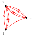
Figure 1: The state graph of $W=\{(12132),(12321)\}$ and $\overline{W}=\{(13212),(21232)\}$.

From the definition of state graph it is clear that it records the transitions in a given multiset of words and we state the following proposition.

Proposition 1 (Proposition 2.1 in Haws:2011fk )

Let $A^{T}$ be the design matrix for the THMC, and $W,\overline{W}\in{\mathcal{P}^{*}}(\Omega_{S,T})$. Then $A^{T}(W)=A^{T}(\overline{W})$ if and only if $G(W)=G(\overline{W})$.

Throughout this paper we alternate between terminology of the multiset of words $W$ and the graph $G(W)$ it defines.

3 Facets of the design polytope

3.1 Polytopes

We recall some necessary definitions from polyhedral geometry and we refer the reader to the book of Schrijver Schrijver1986Theory-of-linea for more details. The convex hull of $\{\mathchoice{\mbox{\boldmath$\displaystyle\bf a$}}{\mbox{\boldmath$\textstyle\bf a$}}{\mbox{\boldmath$\scriptstyle\bf a$}}{\mbox{\boldmath$\scriptscriptstyle\bf a$}}_{1},\ldots,\mathchoice{\mbox{\boldmath$\displaystyle\bf a$}}{\mbox{\boldmath$\textstyle\bf a$}}{\mbox{\boldmath$\scriptstyle\bf a$}}{\mbox{\boldmath$\scriptscriptstyle\bf a$}}_{m}\}\subset{\mathbb{R}}^{d}$ is defined as

$$\operatorname{conv}(\mathchoice{\mbox{\boldmath$\displaystyle\bf a$}}{\mbox{\boldmath$\textstyle\bf a$}}{\mbox{\boldmath$\scriptstyle\bf a$}}{\mbox{\boldmath$\scriptscriptstyle\bf a$}}_{1},\ldots,\mathchoice{\mbox{\boldmath$\displaystyle\bf a$}}{\mbox{\boldmath$\textstyle\bf a$}}{\mbox{\boldmath$\scriptstyle\bf a$}}{\mbox{\boldmath$\scriptscriptstyle\bf a$}}_{m}):=\left\{\,\mathchoice{\mbox{\boldmath$\displaystyle\bf x$}}{\mbox{\boldmath$\textstyle\bf x$}}{\mbox{\boldmath$\scriptstyle\bf x$}}{\mbox{\boldmath$\scriptscriptstyle\bf x$}}\in{\mathbb{R}}^{d}\mid\mathchoice{\mbox{\boldmath$\displaystyle\bf x$}}{\mbox{\boldmath$\textstyle\bf x$}}{\mbox{\boldmath$\scriptstyle\bf x$}}{\mbox{\boldmath$\scriptscriptstyle\bf x$}}=\sum_{i=1}^{m}\lambda_{i}\mathchoice{\mbox{\boldmath$\displaystyle\bf a$}}{\mbox{\boldmath$\textstyle\bf a$}}{\mbox{\boldmath$\scriptstyle\bf a$}}{\mbox{\boldmath$\scriptscriptstyle\bf a$}}_{i},\,\,\sum_{i=1}^{m}\lambda_{i}=1,\,\lambda_{i}\geq 0\,\right\}.$$

A polytope ${P}$ is the convex hull of finitely many points. We say $F\subseteq{P}$ is a face of the polytope ${P}$ if there exists a vector $\textstyle\bf c$ such that $F=\arg\max_{\mathchoice{\mbox{\boldmath$\displaystyle\bf x$}}{\mbox{\boldmath$\textstyle\bf x$}}{\mbox{\boldmath$\scriptstyle\bf x$}}{\mbox{\boldmath$\scriptscriptstyle\bf x$}}\in{P}}\mathchoice{\mbox{\boldmath$\displaystyle\bf c$}}{\mbox{\boldmath$\textstyle\bf c$}}{\mbox{\boldmath$\scriptstyle\bf c$}}{\mbox{\boldmath$\scriptscriptstyle\bf c$}}\cdot\mathchoice{\mbox{\boldmath$\displaystyle\bf x$}}{\mbox{\boldmath$\textstyle\bf x$}}{\mbox{\boldmath$\scriptstyle\bf x$}}{\mbox{\boldmath$\scriptscriptstyle\bf x$}}$. Every face $F$ of ${P}$ is also a polytope. If ${P}$ is of dimension $D$, a face $F$ of dimension $D{-}1$ is a called a facet. For $k\in{\mathbb{N}}$, we define the $k$-th dilation of $P$ as $k{P}:=\left\{\,k\mathchoice{\mbox{\boldmath$\displaystyle\bf x$}}{\mbox{\boldmath$\textstyle\bf x$}}{\mbox{\boldmath$\scriptstyle\bf x$}}{\mbox{\boldmath$\scriptscriptstyle\bf x$}}\mid\mathchoice{\mbox{\boldmath$\displaystyle\bf x$}}{\mbox{\boldmath$\textstyle\bf x$}}{\mbox{\boldmath$\scriptstyle\bf x$}}{\mbox{\boldmath$\scriptscriptstyle\bf x$}}\in{P}\right\}$. A point $\mathchoice{\mbox{\boldmath$\displaystyle\bf x$}}{\mbox{\boldmath$\textstyle\bf x$}}{\mbox{\boldmath$\scriptstyle\bf x$}}{\mbox{\boldmath$\scriptscriptstyle\bf x$}}\in{P}$ is a vertex if it can not be written as a convex combination of points from ${P}\backslash\{\mathchoice{\mbox{\boldmath$\displaystyle\bf x$}}{\mbox{\boldmath$\textstyle\bf x$}}{\mbox{\boldmath$\scriptstyle\bf x$}}{\mbox{\boldmath$\scriptscriptstyle\bf x$}}\}$.

The cone of $\{\mathchoice{\mbox{\boldmath$\displaystyle\bf a$}}{\mbox{\boldmath$\textstyle\bf a$}}{\mbox{\boldmath$\scriptstyle\bf a$}}{\mbox{\boldmath$\scriptscriptstyle\bf a$}}_{1},\ldots,\mathchoice{\mbox{\boldmath$\displaystyle\bf a$}}{\mbox{\boldmath$\textstyle\bf a$}}{\mbox{\boldmath$\scriptstyle\bf a$}}{\mbox{\boldmath$\scriptscriptstyle\bf a$}}_{m}\}\subset{\mathbb{R}}^{d}$ is defined as

$$\operatorname{cone}(\mathchoice{\mbox{\boldmath$\displaystyle\bf a$}}{\mbox{\boldmath$\textstyle\bf a$}}{\mbox{\boldmath$\scriptstyle\bf a$}}{\mbox{\boldmath$\scriptscriptstyle\bf a$}}_{1},\ldots,\mathchoice{\mbox{\boldmath$\displaystyle\bf a$}}{\mbox{\boldmath$\textstyle\bf a$}}{\mbox{\boldmath$\scriptstyle\bf a$}}{\mbox{\boldmath$\scriptscriptstyle\bf a$}}_{m}):=\left\{\,\mathchoice{\mbox{\boldmath$\displaystyle\bf x$}}{\mbox{\boldmath$\textstyle\bf x$}}{\mbox{\boldmath$\scriptstyle\bf x$}}{\mbox{\boldmath$\scriptscriptstyle\bf x$}}\in{\mathbb{R}}^{d}\mid\mathchoice{\mbox{\boldmath$\displaystyle\bf x$}}{\mbox{\boldmath$\textstyle\bf x$}}{\mbox{\boldmath$\scriptstyle\bf x$}}{\mbox{\boldmath$\scriptscriptstyle\bf x$}}=\sum_{i=1}^{m}\lambda_{i}\mathchoice{\mbox{\boldmath$\displaystyle\bf a$}}{\mbox{\boldmath$\textstyle\bf a$}}{\mbox{\boldmath$\scriptstyle\bf a$}}{\mbox{\boldmath$\scriptscriptstyle\bf a$}}_{i},\,\lambda_{i}\geq 0\,\right\}.$$

Thus, $\operatorname{cone}(A)$ denote the cone over the columns of a matrix $A$. We are interested in the case when the matrix in consideration is the design matrix $A^{T}$. We define the design polytope ${P}^{T}$ as the convex hull $\operatorname{conv}(A^{T})$ and we write $C^{T}$ to denote $\operatorname{cone}(A^{T})$.

Given an integer matrix $A\in{\mathbb{Z}}^{d\times m}$ we associate an integer lattice ${\mathbb{Z}}A=\{n_{1}\mathchoice{\mbox{\boldmath$\displaystyle\bf a$}}{\mbox{\boldmath$\textstyle\bf a$}}{\mbox{\boldmath$\scriptstyle\bf a$}}{\mbox{\boldmath$\scriptscriptstyle\bf a$}}_{1}+\cdots+n_{m}\mathchoice{\mbox{\boldmath$\displaystyle\bf a$}}{\mbox{\boldmath$\textstyle\bf a$}}{\mbox{\boldmath$\scriptstyle\bf a$}}{\mbox{\boldmath$\scriptscriptstyle\bf a$}}_{m}\mid n_{i}\in{\mathbb{Z}}\}$. We can also associate the semigroup ${\mathbb{N}}A:=\{n_{1}\mathchoice{\mbox{\boldmath$\displaystyle\bf a$}}{\mbox{\boldmath$\textstyle\bf a$}}{\mbox{\boldmath$\scriptstyle\bf a$}}{\mbox{\boldmath$\scriptscriptstyle\bf a$}}_{1}+\cdots+n_{m}\mathchoice{\mbox{\boldmath$\displaystyle\bf a$}}{\mbox{\boldmath$\textstyle\bf a$}}{\mbox{\boldmath$\scriptstyle\bf a$}}{\mbox{\boldmath$\scriptscriptstyle\bf a$}}_{m}\mid n_{i}\in{\mathbb{N}}\}$. We say that the semigroup ${\mathbb{N}}A$ is normal when $\mathchoice{\mbox{\boldmath$\displaystyle\bf x$}}{\mbox{\boldmath$\textstyle\bf x$}}{\mbox{\boldmath$\scriptstyle\bf x$}}{\mbox{\boldmath$\scriptscriptstyle\bf x$}}\in{\mathbb{N}}A$ if and only if there exist $\mathchoice{\mbox{\boldmath$\displaystyle\bf y$}}{\mbox{\boldmath$\textstyle\bf y$}}{\mbox{\boldmath$\scriptstyle\bf y$}}{\mbox{\boldmath$\scriptscriptstyle\bf y$}}\in{\mathbb{Z}}^{m}$ and $\alpha\in{\mathbb{R}}_{\geq 0}^{m}$ such that $\mathchoice{\mbox{\boldmath$\displaystyle\bf x$}}{\mbox{\boldmath$\textstyle\bf x$}}{\mbox{\boldmath$\scriptstyle\bf x$}}{\mbox{\boldmath$\scriptscriptstyle\bf x$}}=A\mathchoice{\mbox{\boldmath$\displaystyle\bf y$}}{\mbox{\boldmath$\textstyle\bf y$}}{\mbox{\boldmath$\scriptstyle\bf y$}}{\mbox{\boldmath$\scriptscriptstyle\bf y$}}$ and $\mathchoice{\mbox{\boldmath$\displaystyle\bf x$}}{\mbox{\boldmath$\textstyle\bf x$}}{\mbox{\boldmath$\scriptstyle\bf x$}}{\mbox{\boldmath$\scriptscriptstyle\bf x$}}=A\alpha$. The set ${\mathbb{Z}}A\cap\operatorname{cone}(A)$ is called the saturation of ${\mathbb{N}}A$. See MS2005 ; Sturmfels1996 for more details on normality.

If $\mathchoice{\mbox{\boldmath$\displaystyle\bf x$}}{\mbox{\boldmath$\textstyle\bf x$}}{\mbox{\boldmath$\scriptstyle\bf x$}}{\mbox{\boldmath$\scriptscriptstyle\bf x$}}\in{\mathbb{R}}^{6}$, we index $\textstyle\bf x$ by $\{\,ij\mid 1\leq i,j\leq 3,\,i\neq j\,\}$. We define $\mathchoice{\mbox{\boldmath$\displaystyle\bf e$}}{\mbox{\boldmath$\textstyle\bf e$}}{\mbox{\boldmath$\scriptstyle\bf e$}}{\mbox{\boldmath$\scriptscriptstyle\bf e$}}_{ij}\in{\mathbb{R}}^{6}$ to be the vector of all zeros, except $1$ at index $ij$. We also adopt the notation $x_{i+}:=\sum_{j}x_{ij}$ and $x_{+i}:=\sum_{j}x_{ji}$. For any $\mathchoice{\mbox{\boldmath$\displaystyle\bf x$}}{\mbox{\boldmath$\textstyle\bf x$}}{\mbox{\boldmath$\scriptstyle\bf x$}}{\mbox{\boldmath$\scriptscriptstyle\bf x$}}\in{\mathbb{N}}^{6}$ we can define a directed multigraph $G(\mathchoice{\mbox{\boldmath$\displaystyle\bf x$}}{\mbox{\boldmath$\textstyle\bf x$}}{\mbox{\boldmath$\scriptstyle\bf x$}}{\mbox{\boldmath$\scriptscriptstyle\bf x$}})$ on three vertices, where there are $x_{ij}$ directed edges from vertex $i$ to vertex $j$. One would like to identify the vectors $\mathchoice{\mbox{\boldmath$\displaystyle\bf x$}}{\mbox{\boldmath$\textstyle\bf x$}}{\mbox{\boldmath$\scriptstyle\bf x$}}{\mbox{\boldmath$\scriptscriptstyle\bf x$}}\in{\mathbb{N}}^{6}$ for which the graph $G(\mathchoice{\mbox{\boldmath$\displaystyle\bf x$}}{\mbox{\boldmath$\textstyle\bf x$}}{\mbox{\boldmath$\scriptstyle\bf x$}}{\mbox{\boldmath$\scriptscriptstyle\bf x$}})$ is a state graph. Nevertheless, observe that $x_{i+}$ is the out-degree of vertex $i$ and $x_{+i}$ is the in-degree of vertex $i$ with respect to $G(\mathchoice{\mbox{\boldmath$\displaystyle\bf x$}}{\mbox{\boldmath$\textstyle\bf x$}}{\mbox{\boldmath$\scriptstyle\bf x$}}{\mbox{\boldmath$\scriptscriptstyle\bf x$}})$.

We now give some properties which will be used later for describing the facets of the design polytope ${P}^{T}$ given by the design matrix for our model, and to prove normality of the semigroup associated with the design matrix.

Proposition 2 (Proposition 5.1 in Haws:2011fk )

Let $A^{T}$ be the design matrix for the THMC without loops and initial parameters. If $\mathchoice{\mbox{\boldmath$\displaystyle\bf x$}}{\mbox{\boldmath$\textstyle\bf x$}}{\mbox{\boldmath$\scriptstyle\bf x$}}{\mbox{\boldmath$\scriptscriptstyle\bf x$}}\in{\mathbb{Z}}A^{T}\cap C^{T}$ then $\sum_{i\neq j}x_{ij}=n(T{-}1)$ for some $n\in{\mathbb{N}}$ and $|x_{i+}-x_{+i}|\leq n$ for all $i\in\{1,2,3\}$.

An immediate consequence of this proposition is that ${P}^{T}\subset{\mathbb{R}}^{6}$ has dimension 5. Proposition 2 also states that for $\mathchoice{\mbox{\boldmath$\displaystyle\bf x$}}{\mbox{\boldmath$\textstyle\bf x$}}{\mbox{\boldmath$\scriptstyle\bf x$}}{\mbox{\boldmath$\scriptscriptstyle\bf x$}}\in{\mathbb{Z}}A^{T}\cap C^{T}$ the multigraph $G(\mathchoice{\mbox{\boldmath$\displaystyle\bf x$}}{\mbox{\boldmath$\textstyle\bf x$}}{\mbox{\boldmath$\scriptstyle\bf x$}}{\mbox{\boldmath$\scriptscriptstyle\bf x$}})$ will have in-degree and out-degree bounded by $\|\mathchoice{\mbox{\boldmath$\displaystyle\bf x$}}{\mbox{\boldmath$\textstyle\bf x$}}{\mbox{\boldmath$\scriptstyle\bf x$}}{\mbox{\boldmath$\scriptscriptstyle\bf x$}}\|_{1}/(T{-}1)$ at every vertex. This implies nice properties when $\|\mathchoice{\mbox{\boldmath$\displaystyle\bf x$}}{\mbox{\boldmath$\textstyle\bf x$}}{\mbox{\boldmath$\scriptstyle\bf x$}}{\mbox{\boldmath$\scriptscriptstyle\bf x$}}\|_{1}=(T{-}1)$. Recall that a path in a directed multigraph is Eulerian if it visits every edge only once.

Proposition 3 (Proposition 5.2 in Haws:2011fk )

If $G$ is a directed multigraph on three vertices, with no self-loops, $T{-}1$ edges, and satisfying

$$|G_{i+}-G_{+i}|\leq 1\qquad\,i=1,2,3;$$

then, there exists an Eulerian path in $G$.

Note that every word $\mathchoice{\mbox{\boldmath$\displaystyle\bf w$}}{\mbox{\boldmath$\textstyle\bf w$}}{\mbox{\boldmath$\scriptstyle\bf w$}}{\mbox{\boldmath$\scriptscriptstyle\bf w$}}\in{\mathcal{P}^{*}}(\Omega_{T})$ gives an Eulerian path in $G(\{\mathchoice{\mbox{\boldmath$\displaystyle\bf w$}}{\mbox{\boldmath$\textstyle\bf w$}}{\mbox{\boldmath$\scriptstyle\bf w$}}{\mbox{\boldmath$\scriptscriptstyle\bf w$}}\})$ containing all edges. Conversely, for every multigraph $G$ with an Eulerian path containing all edges, there exists $\mathchoice{\mbox{\boldmath$\displaystyle\bf w$}}{\mbox{\boldmath$\textstyle\bf w$}}{\mbox{\boldmath$\scriptstyle\bf w$}}{\mbox{\boldmath$\scriptscriptstyle\bf w$}}\in{\mathcal{P}^{*}}(\Omega_{T})$ such that $G(\{\mathchoice{\mbox{\boldmath$\displaystyle\bf w$}}{\mbox{\boldmath$\textstyle\bf w$}}{\mbox{\boldmath$\scriptstyle\bf w$}}{\mbox{\boldmath$\scriptscriptstyle\bf w$}}$})$=G$. More specifically, $\textstyle\bf w$ is the Eulerian path in $G(\{\mathchoice{\mbox{\boldmath$\displaystyle\bf w$}}{\mbox{\boldmath$\textstyle\bf w$}}{\mbox{\boldmath$\scriptstyle\bf w$}}{\mbox{\boldmath$\scriptscriptstyle\bf w$}}\})$. Throughout this paper we use the terms path and word interchangeably.

Lemma 3.1 (Lemma 5.2 in Haws:2011fk )

Let $A^{T}$ be the design matrix for the THMC. If $T\geq 4$, then ${P}^{T}\cap{\mathbb{Z}}^{6}=A^{T}$, where the right hand side is taken as the set of columns of the matrix $A^{T}$.

We define

$$H_{n(T{-}1)}:=\left\{\mathchoice{\mbox{\boldmath$\displaystyle\bf x$}}{\mbox{\boldmath$\textstyle\bf x$}}{\mbox{\boldmath$\scriptstyle\bf x$}}{\mbox{\boldmath$\scriptscriptstyle\bf x$}}\in{\mathbb{R}}^{6}\mid\sum_{i\neq j}x_{ij}=n(T{-}1)\right\}.$$

Proposition 4 (Proposition 5.3 in Haws:2011fk )

Let $A^{T}$ be the design matrix for the THMC without initial parameters and no loops.

1. For $T\geq 4$ and $n\in{\mathbb{N}}$,

   $$n{P}^{T}=C^{T}\cap H_{n(T-1)}.$$

2. For $T\geq 4$,

   $$C^{T}\cap{\mathbb{Z}}A^{T}=\bigoplus_{n=0}^{\infty}\left(n{P}^{T}\cap{\mathbb{Z}}^{6}\right).$$

3.2 Facets of ${P}^{T}$ for $T\geq 5$

In this section we describe the facets of the design polytope ${P}^{T}$ for arbitrary $T\geq 5$. For $T=3,4$ it can be easily checked that ${P}^{T}$ has 12 facets using Polymake polymake . For $T\geq 5$ the output of Polymake suggests that ${P}^{T}$ always has 24 facets. In the following we establish this fact by explicitly describing all these facets for all $T\geq 5$.

Recall that vectors $\mathchoice{\mbox{\boldmath$\displaystyle\bf c$}}{\mbox{\boldmath$\textstyle\bf c$}}{\mbox{\boldmath$\scriptstyle\bf c$}}{\mbox{\boldmath$\scriptscriptstyle\bf c$}}\in{\mathbb{R}}^{6}$ are indexed as $[c_{12},c_{13},c_{21},c_{23},c_{31},c_{32}]$. The proofs for the facets of ${P}^{T}$ rely heavily on the state graph. Note that we give the facets of the design polytope in terms of equivalence classes under permutations of the labels $\{1,2,3\}$. For example, if $\mathfrak{S}_{3}$ denotes the set of permutations of the set $\{1,2,3\}$ and if the vector $[c_{12},c_{13},c_{21},c_{23},c_{31},c_{32}]$ defines a facet, then for any $\sigma\in\mathfrak{S}_{3}$, the vector

$$[c_{\sigma(1)\sigma(2)},c_{\sigma(1)\sigma(3)},c_{\sigma(2)\sigma(1)},c_{\sigma(2)\sigma(3)},c_{\sigma(3)\sigma(1)},c_{\sigma(3)\sigma(2)}]$$

also defines a facet. Also note that, due to Proposition 4, the facets of the polytope ${P}^{T}$ and the cone $C^{T}$ are not only in bijection but they can be determined by the same linear inequalities of the form $\mathchoice{\mbox{\boldmath$\displaystyle\bf c$}}{\mbox{\boldmath$\textstyle\bf c$}}{\mbox{\boldmath$\scriptstyle\bf c$}}{\mbox{\boldmath$\scriptscriptstyle\bf c$}}\cdot\mathchoice{\mbox{\boldmath$\displaystyle\bf x$}}{\mbox{\boldmath$\textstyle\bf x$}}{\mbox{\boldmath$\scriptstyle\bf x$}}{\mbox{\boldmath$\scriptscriptstyle\bf x$}}\geq 0$. We call $\textstyle\bf c$ the vector defining a facet of ${P}^{T}$ or $C^{T}$.

Recall that in general, to show that a vector $\textstyle\bf c$ defines a facet of $C^{T}$, we need to show the following two things:

• (Non-negativity) $\mathchoice{\mbox{\boldmath$\displaystyle\bf c$}}{\mbox{\boldmath$\textstyle\bf c$}}{\mbox{\boldmath$\scriptstyle\bf c$}}{\mbox{\boldmath$\scriptscriptstyle\bf c$}}\cdot\mathchoice{\mbox{\boldmath$\displaystyle\bf a$}}{\mbox{\boldmath$\textstyle\bf a$}}{\mbox{\boldmath$\scriptstyle\bf a$}}{\mbox{\boldmath$\scriptscriptstyle\bf a$}}^{T}_{\mathchoice{\mbox{\boldmath$\displaystyle\bf w$}}{\mbox{\boldmath$\textstyle\bf w$}}{\mbox{\boldmath$\scriptstyle\bf w$}}{\mbox{\boldmath$\scriptscriptstyle\bf w$}}}$ are non-negative for all $\mathchoice{\mbox{\boldmath$\displaystyle\bf w$}}{\mbox{\boldmath$\textstyle\bf w$}}{\mbox{\boldmath$\scriptstyle\bf w$}}{\mbox{\boldmath$\scriptscriptstyle\bf w$}}\in\Omega_{T}$.

• (Dimensionality) the dimension of linear subspace spanned by $\{\mathchoice{\mbox{\boldmath$\displaystyle\bf a$}}{\mbox{\boldmath$\textstyle\bf a$}}{\mbox{\boldmath$\scriptstyle\bf a$}}{\mbox{\boldmath$\scriptscriptstyle\bf a$}}^{T}_{\mathchoice{\mbox{\boldmath$\displaystyle\bf w$}}{\mbox{\boldmath$\textstyle\bf w$}}{\mbox{\boldmath$\scriptstyle\bf w$}}{\mbox{\boldmath$\scriptscriptstyle\bf w$}}}\mid\mathchoice{\mbox{\boldmath$\displaystyle\bf c$}}{\mbox{\boldmath$\textstyle\bf c$}}{\mbox{\boldmath$\scriptstyle\bf c$}}{\mbox{\boldmath$\scriptscriptstyle\bf c$}}\cdot\mathchoice{\mbox{\boldmath$\displaystyle\bf a$}}{\mbox{\boldmath$\textstyle\bf a$}}{\mbox{\boldmath$\scriptstyle\bf a$}}{\mbox{\boldmath$\scriptscriptstyle\bf a$}}^{T}_{\mathchoice{\mbox{\boldmath$\displaystyle\bf w$}}{\mbox{\boldmath$\textstyle\bf w$}}{\mbox{\boldmath$\scriptstyle\bf w$}}{\mbox{\boldmath$\scriptscriptstyle\bf w$}}}=0\}$ is $5$.

Proposition 5

For any $T\geq 5$

$$\mathchoice{\mbox{\boldmath$\displaystyle\bf c$}}{\mbox{\boldmath$\textstyle\bf c$}}{\mbox{\boldmath$\scriptstyle\bf c$}}{\mbox{\boldmath$\scriptscriptstyle\bf c$}}=[1,0,0,0,0,0]$$

defines a facet of ${P}^{T}$ modulo $\mathfrak{S}_{3}$.

Proof

The non-negativity i) follows by definition, as the transition count between states should be a non-negative integer. Now, for dimensionality ii), consider the following four paths

$$2313\cdots 13,\ 1323\cdots 23,\ 3232\cdots 32,\ 3131\cdots 31.$$ (3.1)

These paths have sufficient statistics that depend on $T$. The vectors of sufficient statistics for $T=2k$ are

$$[0,k{-}1,0,1,k{-}1,0],\;[0,1,0,k{-}1,0,k{-}1],\;[0,0,0,k{-}1,0,k],\;[0,k{-}1,0,0,k,0];$$

and when $T=2k+1$ the sufficient statistics are

$$[0,k{-}1,0,1,k,0],\;[0,1,0,k{-}1,0,k],\;[0,0,0,k,0,k],\;[0,k,0,0,k,0].$$

Thus, the four paths in (3.1) correspond to four vectors that are linearly independent for $T\geq 5$. Lastly, consider the following path

$$132132\cdots 132.$$

Its vector of transition counts contains a nonzero value in the coordinate corresponding to the transition $21$, which shows that the space generated by the transition counts of these five paths is 5-dimensional. We conclude by noticing that none of these paths contain the transition $12$, thus they satisfy $\mathchoice{\mbox{\boldmath$\displaystyle\bf c$}}{\mbox{\boldmath$\textstyle\bf c$}}{\mbox{\boldmath$\scriptstyle\bf c$}}{\mbox{\boldmath$\scriptscriptstyle\bf c$}}\cdot\mathchoice{\mbox{\boldmath$\displaystyle\bf a$}}{\mbox{\boldmath$\textstyle\bf a$}}{\mbox{\boldmath$\scriptstyle\bf a$}}{\mbox{\boldmath$\scriptscriptstyle\bf a$}}^{T}_{\mathchoice{\mbox{\boldmath$\displaystyle\bf w$}}{\mbox{\boldmath$\textstyle\bf w$}}{\mbox{\boldmath$\scriptstyle\bf w$}}{\mbox{\boldmath$\scriptscriptstyle\bf w$}}}=0$.

Proposition 6

For any $T\geq 5$

$$\mathchoice{\mbox{\boldmath$\displaystyle\bf c$}}{\mbox{\boldmath$\textstyle\bf c$}}{\mbox{\boldmath$\scriptstyle\bf c$}}{\mbox{\boldmath$\scriptscriptstyle\bf c$}}=[T,\,T,\,-(T{-}2),\,1,\,-(T{-}2),\,1]$$

defines a facet of ${P}^{T}$ modulo $\mathfrak{S}_{3}$.

Proof

We check the non-negativity i). Consider any particular word (path) $\mathchoice{\mbox{\boldmath$\displaystyle\bf w$}}{\mbox{\boldmath$\textstyle\bf w$}}{\mbox{\boldmath$\scriptstyle\bf w$}}{\mbox{\boldmath$\scriptscriptstyle\bf w$}}\in\Omega_{T}$ of length $T$ with transition counts $x_{12},x_{13},x_{21},x_{23},x_{31},x_{32}$. We need to show

$$T(x_{12}+x_{13})+x_{23}+x_{32}\geq(T{-}2)(x_{21}+x_{31}).$$ (3.2)

Note that $x_{12}+x_{13}$ is the out-degree of vertex 1 and $x_{21}+x_{31}$ is the in-degree of vertex 1 with respect to the graph $G(\mathchoice{\mbox{\boldmath$\displaystyle\bf w$}}{\mbox{\boldmath$\textstyle\bf w$}}{\mbox{\boldmath$\scriptstyle\bf w$}}{\mbox{\boldmath$\scriptscriptstyle\bf w$}})$. By Proposition 2 the out-degree and the in-degree can differ by at most $1$. Note that (3.2) trivially holds when $x_{12}+x_{13}\geq x_{21}+x_{31}$. Hence we only need to check the case $a=x_{12}+x_{13}=x_{21}+x_{31}-1$. Now

$$T{-}1=x_{12}+x_{13}+x_{21}+x_{23}+x_{31}+x_{32}=2a+1+x_{23}+x_{32}$$

or

$$2a+2+x_{23}+x_{32}-T=0.$$

Hence the difference of two sides of (3.2) is written as

$$Ta+x_{23}+x_{32}-(T{-}2)(a+1)=x_{23}+x_{32}+2(a{+}1)-T=0.$$ (3.3)

This proves the non-negativity.

Next we consider dimensionality ii). Equation (3.2) can not hold with equality in the case $x_{12}+x_{13}>x_{21}+x_{31}$. Also (3.2) can not hold with equality in the case $x_{12}+x_{13}=x_{21}+x_{31}>0$. Furthermore, if $0=x_{12}+x_{13}=x_{21}+x_{31}$, then the path entirely consists of edges between 2 and 3. Then $T{-}1=x_{32}+x_{23}>0$ and (3.2) does not hold with equality. Hence the only remaining case is $x_{12}+x_{13}=x_{21}+x_{31}-1$. But then, from (3.3) we see that (3.2) holds with equality. Therefore, all paths $\textstyle\bf w$ such that $x_{12}+x_{13}=x_{21}+x_{31}-1$ satisfies $\mathchoice{\mbox{\boldmath$\displaystyle\bf c$}}{\mbox{\boldmath$\textstyle\bf c$}}{\mbox{\boldmath$\scriptstyle\bf c$}}{\mbox{\boldmath$\scriptscriptstyle\bf c$}}\cdot\mathchoice{\mbox{\boldmath$\displaystyle\bf a$}}{\mbox{\boldmath$\textstyle\bf a$}}{\mbox{\boldmath$\scriptstyle\bf a$}}{\mbox{\boldmath$\scriptscriptstyle\bf a$}}_{\mathchoice{\mbox{\boldmath$\displaystyle\bf w$}}{\mbox{\boldmath$\textstyle\bf w$}}{\mbox{\boldmath$\scriptstyle\bf w$}}{\mbox{\boldmath$\scriptscriptstyle\bf w$}}}^{T}=0$. We now give five such paths with linearly independent sufficient statistics, which depends on $T\bmod 3$ and $T\bmod 2$.

If $T$ even, consider

$$3131\cdots 131,\;2121\cdots 121,\;3232\cdots 3231$$

If $T$ odd, consider

$$23131\cdots 31,\;32121\cdots 21,\;2323\cdots 231$$

If $T\equiv 0\ \pmod{3}$, consider

$$321321\cdots 321,\;231231\cdots 231$$

If $T\equiv 2\pmod{3}$, consider

$$213213\cdots 2131,\;312312\cdots 3121$$

Finally if $T\equiv 1\pmod{3}$, put the loop $232$ or $323$ in front of the word above for the value of $T\equiv 2\pmod{3}$.

We need to show that the sufficient statistics of these paths are linearly independent. For example, consider the case $T=6k$. Then the sufficient statistics are given by the vectors

$$[0,3k{-}1,0,0,3k,0],\;[3k{-}1,0,3k,0,0,0],\;[0,0,0,3k{-}1,1,3k{-}1],$$

$$[0,2k{-}1,2k,0,0,2k],\;[0,2k,0,2k{-}1,2k,0].$$

For $k\geq 1$, the linear independence of these five vectors can be easily verified. Other cases $T\equiv r\pmod{6}$ can be similarly handled.

In a similar fashion, we prove the following propositions.

Proposition 7

For any $T=2k+1$ odd, $T\geq 5$,

$$\mathchoice{\mbox{\boldmath$\displaystyle\bf c$}}{\mbox{\boldmath$\textstyle\bf c$}}{\mbox{\boldmath$\scriptstyle\bf c$}}{\mbox{\boldmath$\scriptscriptstyle\bf c$}}=[1,\,1,\,-1,\,-1,\,1,\,1]$$

defines a facet of ${P}^{T}$ modulo $\mathfrak{S}_{3}$.

Proof

For non-negativity, consider

$$x_{12}+x_{13}+x_{31}+x_{32}\geq x_{21}+x_{23}.$$ (3.4)

We can “merge” two vertices 1 and 3 as a virtual vertex 4 and consider 4 as a single vertex. Then the resulting graph has only two vertices (2 and 4). Then $x_{12}+x_{32}$ is the out-degree of this vertex 4. If $x_{12}+x_{32}\geq x_{21}+x_{23}$ then the inequality is trivial. Consider the case $x_{12}+x_{32}=x_{21}+x_{23}-1$. We need to show that in this case we have $x_{13}+x_{31}\geq 1$. By contradiction assume that $x_{13}+x_{31}=0$. Then the path of odd length is like

$$2424242.$$

However in this case $x_{12}+x_{32}=x_{21}+x_{23}$, which is a contradiction. Therefore we have proved that (3.4) holds for any path $\textstyle\bf w$.

Now we check the dimensionality ii). In order to check the dimensionality we verify for which path (3.4) holds with equality. The first case is $0=x_{13}+x_{31}$. Then as we saw above we have $x_{12}+x_{32}=x_{21}+x_{23}$. Other case is $1=x_{13}+x_{31}$, i.e. either $x_{13}=1,x_{31}=0$ or $x_{31}=1,x_{13}=0$. In the former case the path is like

$$2121323$$

and in the latter case the path is like $2323121$. We claim that for $T=2k+1\geq 5$ the paths

$$121\cdots 121,\;232\cdots 232,\;212\cdots 2123,\;1323\cdots 232,\;3121\cdots 212$$

give sufficient statistics that are linearly independent and hold with equality for Equation (3.4). The sufficient statistics for the paths above are

$$[k,0,k,0,0,0],\;[0,0,0,k,0,k],\;[k{-}1,1,k,0,0,0],$$

$$[0,1,0,k{-}1,0,k],\;[k,0,k{-}1,0,1,0].$$

For $k\geq 2$, one can check the linear independence of these 5 vectors.

We now consider any three consecutive transitions, or a path for $T=4$. Let $\tilde{x}_{ij}$, $1\leq i\neq j\leq 3$, be transition counts of these three transitions.

Lemma 3.2

Let $i,j,t$ be distinct (i.e.  $\{i,j,t\}=\{1,2,3\}$). Then

$$\tilde{x}_{ij}+\tilde{x}_{jt}+\tilde{x}_{it}\geq 1.$$

Proof

Suppose that $\tilde{x}_{ij}+\tilde{x}_{jt}+\tilde{x}_{it}=0$. Then in the three transitions, we can not use the directed edges $ij$, $jt$, $it$. Then the available edges are $ji,ti,tj$. By drawing a state graph, it is obvious that by the edges $ji,ti,tj$ only, we can not form a path of three transitions.

Proposition 8

For any $T\geq 7$ of the form $T=3k{+}1$ ($k\geq 2$),

$$\mathchoice{\mbox{\boldmath$\displaystyle\bf c$}}{\mbox{\boldmath$\textstyle\bf c$}}{\mbox{\boldmath$\scriptstyle\bf c$}}{\mbox{\boldmath$\scriptscriptstyle\bf c$}}=[2,\,-1,\,-1,\,-1,\,2,\,2]$$

defines a facet of ${P}^{T}$ modulo $\mathfrak{S}_{3}$.

Proof

For non-negativity, consider the inequality

$$2(x_{12}+x_{31}+x_{32})\geq x_{13}+x_{21}+x_{23}$$ (3.5)

Since $x_{13}+x_{21}+x_{23}=T{-}1-(x_{12}+x_{31}+x_{32})=3k-(x_{12}+x_{31}+x_{32})$, the expression (3.5) is equivalent to

$$x_{12}+x_{31}+x_{32}\geq k.$$ (3.6)

If we consider paths in triples of transitions, (3.6) follows from Lemma 3.2.

Now for checking the dimensionality we consider the case when the inequality (3.6) becomes an equality. By the induction above, if we divide a path into triples of transitions (edges), then in each triple only one of $\tilde{x}_{12},\,\tilde{x}_{31},\,\tilde{x}_{32}$ has to be 1. That is, we proved above that for every three transitions (edges) the left-hand-side of equation (3.6) increases by one. For equality to hold, the LHS can only increase by exactly one. Knowing this, we consider the cases for which three transitions increases the LHS of Equation (3.6) by exactly one. In three transitions, a path can either come back to the same vertex or move to another vertex. In the former case (say $ijti$), the following three loops $1321$,$3213$,$2132$ increases $x_{32}$ by 1. Another case going from $i$ to $j$ in three transitions are of the form

$$ijij,ijtj,itij,$$

where $i,j,t$ are different. Then appropriate ones are only the following ones:

$$2121,1313,2323.$$

Therefore in three transitions, we go $2\rightarrow 1$, $1\rightarrow 3$ or $2\rightarrow 3$. Among these three, the only possible connection is

$$2\rightarrow 1\rightarrow 3$$

(or $2\rightarrow 3$ alone). Then the loops are inserted at any point. Thus, we can consider the following paths

$$\qquad 2121321321\cdots 1321,\,1313213\cdots 3213,\,2323213\cdots 3213,\\ 2132132\cdots 2132,\,2121313\cdots 1313,\qquad$$ (3.7)

with sufficient statistics given by the vectors

$$[1,k{-}1,k{+}1,0,0,k{-}1],\,[0,k{+}1,k{-}1,0,1,k{-}1],\,[0,k{-}1,k{-}1,2,0,k],$$

$$[0,k,k,0,0,k],\,[1,2(k{-}1),2,0,k{-}1,0];$$

respectively. For $k\geq 2$ it is easily checked that these vectors are linearly independent and satisfy Equation (3.6) with equality.

Proposition 9

For any $T\geq 5$ of the form $T=3k{+}2$, $k\geq 1$,

$$\mathchoice{\mbox{\boldmath$\displaystyle\bf c$}}{\mbox{\boldmath$\textstyle\bf c$}}{\mbox{\boldmath$\scriptstyle\bf c$}}{\mbox{\boldmath$\scriptscriptstyle\bf c$}}=[2k{+}1,\,-k,\,-k,\,-k,\,2k{+}1,\,2k{+}1]$$

defines a facet of ${P}^{T}$ modulo $\mathfrak{S}_{3}$.

Proof

For non-negativity, consider

$$(2k{+}1)(x_{12}+x_{31}+x_{32})\geq k(x_{13}+x_{21}+x_{23}).$$ (3.8)

Since $x_{13}+x_{21}+x_{23}=T{-}1-(x_{12}+x_{31}+x_{32})=3k{+}1-(x_{12}+x_{31}+x_{32})$, the inequality (3.8) is equivalent to

$$(2k{+}1)(x_{12}+x_{31}+x_{32})\geq k(3k{+}1-(x_{12}+x_{31}+x_{32})),$$

which simplifies to

$$x_{12}+x_{31}+x_{32}\geq k.$$ (3.9)

For a path of length $3k{+}2$, consider omitting the last transition. Then we have a path of length $3k{+}1$. The inequality already holds for this shortened path by Proposition 8. Since the last transition only increases the transition counts, the same inequality holds for $3k{+}2$. This proves the non-negativity.

For dimensionality, we can find five paths by adding one of the transitions $2\rightarrow 1$, $1\rightarrow 3$, or $2\rightarrow 3$ either at the end or at the beginning of the paths in Proposition 6. In this way, we obtain the following paths

$$2121321321\cdots 1321\underline{3},\,2321321321\cdots 1321\underline{3},\,\underline{2}1313213\cdots 3213,$$

$$\underline{1}3213\cdots 3213,\,2132132\cdots 2132\underline{1},\,$$

with the following vectors of frequencies:

$$[1,k,k{+}1,0,0,k{-}1],\,[0,k,k{+}1,1,0,k{-}1],\,[0,k{+}1,k,0,1,k{-}1],$$

$$[0,k{+}1,k,0,0,k],\,[0,k,k{+}1,0,0,k];$$

which are easily checked to be linearly independent and satisfy (3.9) with equality.

The following lemma will be useful to show the facets of ${P}^{T}$ when $T\geq 6$ is even.

Lemma 3.3

Let $T=2k$, with $k\geq 1$. Then, the inequality $2x_{12}+x_{13}+x_{32}\geq k{-}1$ holds for every path. Moreover, the inequality is strict for every path ending at $s_{T}=2$.

Proof

We prove the lemma by induction on $k$.

For $k=1$, this is a path with a single transition; thus, the statement is obvious, because $2x_{12}+x_{13}+x_{32}$ is non-negative and for two paths $12$, $32$ ending at $s_{2}=2$, we have $2x_{12}+x_{13}+x_{32}=1\ \text{or}\ 2$.

Assume that the proposition holds for $k$. Now we prove that it holds for $k{+}1$. For a path $\textstyle\bf w$ let

$$\bf x = (x_{12},x_{13},x_{21},x_{23},x_{31},x_{32})$$

$$= (x_{12}(\mathchoice{\mbox{\boldmath$\displaystyle\bf w$}}{\mbox{\boldmath$\textstyle\bf w$}}{\mbox{\boldmath$\scriptstyle\bf w$}}{\mbox{\boldmath$\scriptscriptstyle\bf w$}}),x_{13}(\mathchoice{\mbox{\boldmath$\displaystyle\bf w$}}{\mbox{\boldmath$\textstyle\bf w$}}{\mbox{\boldmath$\scriptstyle\bf w$}}{\mbox{\boldmath$\scriptscriptstyle\bf w$}}),x_{21}(\mathchoice{\mbox{\boldmath$\displaystyle\bf w$}}{\mbox{\boldmath$\textstyle\bf w$}}{\mbox{\boldmath$\scriptstyle\bf w$}}{\mbox{\boldmath$\scriptscriptstyle\bf w$}}),x_{23}(\mathchoice{\mbox{\boldmath$\displaystyle\bf w$}}{\mbox{\boldmath$\textstyle\bf w$}}{\mbox{\boldmath$\scriptstyle\bf w$}}{\mbox{\boldmath$\scriptscriptstyle\bf w$}}),x_{31}(\mathchoice{\mbox{\boldmath$\displaystyle\bf w$}}{\mbox{\boldmath$\textstyle\bf w$}}{\mbox{\boldmath$\scriptstyle\bf w$}}{\mbox{\boldmath$\scriptscriptstyle\bf w$}}),x_{32}(\mathchoice{\mbox{\boldmath$\displaystyle\bf w$}}{\mbox{\boldmath$\textstyle\bf w$}}{\mbox{\boldmath$\scriptstyle\bf w$}}{\mbox{\boldmath$\scriptscriptstyle\bf w$}}))$$

denote the transition counts of $\textstyle\bf w$. Consider a path $\textstyle\bf w$ of length $T=2k{+}2$

$$\mathchoice{\mbox{\boldmath$\displaystyle\bf w$}}{\mbox{\boldmath$\textstyle\bf w$}}{\mbox{\boldmath$\scriptstyle\bf w$}}{\mbox{\boldmath$\scriptscriptstyle\bf w$}}=s_{1}\dots s_{2k}s_{2k+1}s_{2k+2}.$$

Denote $\mathchoice{\mbox{\boldmath$\displaystyle\bf w$}}{\mbox{\boldmath$\textstyle\bf w$}}{\mbox{\boldmath$\scriptstyle\bf w$}}{\mbox{\boldmath$\scriptscriptstyle\bf w$}}^{0}=s_{1}\dots s_{2k}$ and $\mathchoice{\mbox{\boldmath$\displaystyle\bf w$}}{\mbox{\boldmath$\textstyle\bf w$}}{\mbox{\boldmath$\scriptstyle\bf w$}}{\mbox{\boldmath$\scriptscriptstyle\bf w$}}^{1}=s_{2k}s_{2k+1}s_{2k+2}$. Then

$$\qquad 2x_{12}(\mathchoice{\mbox{\boldmath$\displaystyle\bf w$}}{\mbox{\boldmath$\textstyle\bf w$}}{\mbox{\boldmath$\scriptstyle\bf w$}}{\mbox{\boldmath$\scriptscriptstyle\bf w$}})+x_{13}(\mathchoice{\mbox{\boldmath$\displaystyle\bf w$}}{\mbox{\boldmath$\textstyle\bf w$}}{\mbox{\boldmath$\scriptstyle\bf w$}}{\mbox{\boldmath$\scriptscriptstyle\bf w$}})+x_{32}(\mathchoice{\mbox{\boldmath$\displaystyle\bf w$}}{\mbox{\boldmath$\textstyle\bf w$}}{\mbox{\boldmath$\scriptstyle\bf w$}}{\mbox{\boldmath$\scriptscriptstyle\bf w$}})=(2x_{12}(\mathchoice{\mbox{\boldmath$\displaystyle\bf w$}}{\mbox{\boldmath$\textstyle\bf w$}}{\mbox{\boldmath$\scriptstyle\bf w$}}{\mbox{\boldmath$\scriptscriptstyle\bf w$}}^{0})+x_{13}(\mathchoice{\mbox{\boldmath$\displaystyle\bf w$}}{\mbox{\boldmath$\textstyle\bf w$}}{\mbox{\boldmath$\scriptstyle\bf w$}}{\mbox{\boldmath$\scriptscriptstyle\bf w$}}^{0})+x_{32}(\mathchoice{\mbox{\boldmath$\displaystyle\bf w$}}{\mbox{\boldmath$\textstyle\bf w$}}{\mbox{\boldmath$\scriptstyle\bf w$}}{\mbox{\boldmath$\scriptscriptstyle\bf w$}}^{0}))\\ +(2x_{12}(\mathchoice{\mbox{\boldmath$\displaystyle\bf w$}}{\mbox{\boldmath$\textstyle\bf w$}}{\mbox{\boldmath$\scriptstyle\bf w$}}{\mbox{\boldmath$\scriptscriptstyle\bf w$}}^{1})+x_{13}(\mathchoice{\mbox{\boldmath$\displaystyle\bf w$}}{\mbox{\boldmath$\textstyle\bf w$}}{\mbox{\boldmath$\scriptstyle\bf w$}}{\mbox{\boldmath$\scriptscriptstyle\bf w$}}^{1})+x_{32}(\mathchoice{\mbox{\boldmath$\displaystyle\bf w$}}{\mbox{\boldmath$\textstyle\bf w$}}{\mbox{\boldmath$\scriptstyle\bf w$}}{\mbox{\boldmath$\scriptscriptstyle\bf w$}}^{1})).\qquad$$

The inductive assumption is that

$$2x_{12}(\mathchoice{\mbox{\boldmath$\displaystyle\bf w$}}{\mbox{\boldmath$\textstyle\bf w$}}{\mbox{\boldmath$\scriptstyle\bf w$}}{\mbox{\boldmath$\scriptscriptstyle\bf w$}}^{0})+x_{13}(\mathchoice{\mbox{\boldmath$\displaystyle\bf w$}}{\mbox{\boldmath$\textstyle\bf w$}}{\mbox{\boldmath$\scriptstyle\bf w$}}{\mbox{\boldmath$\scriptscriptstyle\bf w$}}^{0})+x_{32}(\mathchoice{\mbox{\boldmath$\displaystyle\bf w$}}{\mbox{\boldmath$\textstyle\bf w$}}{\mbox{\boldmath$\scriptstyle\bf w$}}{\mbox{\boldmath$\scriptscriptstyle\bf w$}}^{0})\geq k{-}1$$

and

$$s_{2k}=2\ \Rightarrow\ 2x_{12}(\mathchoice{\mbox{\boldmath$\displaystyle\bf w$}}{\mbox{\boldmath$\textstyle\bf w$}}{\mbox{\boldmath$\scriptstyle\bf w$}}{\mbox{\boldmath$\scriptscriptstyle\bf w$}}^{0})+x_{13}(\mathchoice{\mbox{\boldmath$\displaystyle\bf w$}}{\mbox{\boldmath$\textstyle\bf w$}}{\mbox{\boldmath$\scriptstyle\bf w$}}{\mbox{\boldmath$\scriptscriptstyle\bf w$}}^{0})+x_{32}(\mathchoice{\mbox{\boldmath$\displaystyle\bf w$}}{\mbox{\boldmath$\textstyle\bf w$}}{\mbox{\boldmath$\scriptstyle\bf w$}}{\mbox{\boldmath$\scriptscriptstyle\bf w$}}^{0})\geq k.$$

We prove the first statement of the proposition. If

$$2x_{12}(\mathchoice{\mbox{\boldmath$\displaystyle\bf w$}}{\mbox{\boldmath$\textstyle\bf w$}}{\mbox{\boldmath$\scriptstyle\bf w$}}{\mbox{\boldmath$\scriptscriptstyle\bf w$}}^{1})+x_{13}(\mathchoice{\mbox{\boldmath$\displaystyle\bf w$}}{\mbox{\boldmath$\textstyle\bf w$}}{\mbox{\boldmath$\scriptstyle\bf w$}}{\mbox{\boldmath$\scriptscriptstyle\bf w$}}^{1})+x_{32}(\mathchoice{\mbox{\boldmath$\displaystyle\bf w$}}{\mbox{\boldmath$\textstyle\bf w$}}{\mbox{\boldmath$\scriptstyle\bf w$}}{\mbox{\boldmath$\scriptscriptstyle\bf w$}}^{1})\geq 1,$$

then the inequality holds for ${\bf w}$. On the other hand it is easily seen that if $2x_{12}(\mathchoice{\mbox{\boldmath$\displaystyle\bf w$}}{\mbox{\boldmath$\textstyle\bf w$}}{\mbox{\boldmath$\scriptstyle\bf w$}}{\mbox{\boldmath$\scriptscriptstyle\bf w$}}^{1})+x_{13}(\mathchoice{\mbox{\boldmath$\displaystyle\bf w$}}{\mbox{\boldmath$\textstyle\bf w$}}{\mbox{\boldmath$\scriptstyle\bf w$}}{\mbox{\boldmath$\scriptscriptstyle\bf w$}}^{1})+x_{32}(\mathchoice{\mbox{\boldmath$\displaystyle\bf w$}}{\mbox{\boldmath$\textstyle\bf w$}}{\mbox{\boldmath$\scriptstyle\bf w$}}{\mbox{\boldmath$\scriptscriptstyle\bf w$}}^{1})=0$ then the only possible case is $\mathchoice{\mbox{\boldmath$\displaystyle\bf w$}}{\mbox{\boldmath$\textstyle\bf w$}}{\mbox{\boldmath$\scriptstyle\bf w$}}{\mbox{\boldmath$\scriptscriptstyle\bf w$}}^{1}=231$. Then we have $s_{2k}=2$. Hence by the second part of the inductive assumption we also have the inequality.

We now prove the second statement of the proposition. Let $s_{2k+2}=2$. Note that $s_{2k+1}$ is either 1 or 3. If $s_{2k+1}=1$, then

$$2x_{12}(\mathchoice{\mbox{\boldmath$\displaystyle\bf w$}}{\mbox{\boldmath$\textstyle\bf w$}}{\mbox{\boldmath$\scriptstyle\bf w$}}{\mbox{\boldmath$\scriptscriptstyle\bf w$}}^{1})+x_{13}(\mathchoice{\mbox{\boldmath$\displaystyle\bf w$}}{\mbox{\boldmath$\textstyle\bf w$}}{\mbox{\boldmath$\scriptstyle\bf w$}}{\mbox{\boldmath$\scriptscriptstyle\bf w$}}^{1})+x_{32}(\mathchoice{\mbox{\boldmath$\displaystyle\bf w$}}{\mbox{\boldmath$\textstyle\bf w$}}{\mbox{\boldmath$\scriptstyle\bf w$}}{\mbox{\boldmath$\scriptscriptstyle\bf w$}}^{1})=2$$

and the inequality for $\textstyle\bf w$ is strict. On the other hand let $s_{2k+1}=3$, then there are two cases:

$$\mathchoice{\mbox{\boldmath$\displaystyle\bf w$}}{\mbox{\boldmath$\textstyle\bf w$}}{\mbox{\boldmath$\scriptstyle\bf w$}}{\mbox{\boldmath$\scriptscriptstyle\bf w$}}^{1}=232\ \ \text{or}\ =132.$$

In the former case $2x_{12}(\mathchoice{\mbox{\boldmath$\displaystyle\bf w$}}{\mbox{\boldmath$\textstyle\bf w$}}{\mbox{\boldmath$\scriptstyle\bf w$}}{\mbox{\boldmath$\scriptscriptstyle\bf w$}}^{1})+x_{13}(\mathchoice{\mbox{\boldmath$\displaystyle\bf w$}}{\mbox{\boldmath$\textstyle\bf w$}}{\mbox{\boldmath$\scriptstyle\bf w$}}{\mbox{\boldmath$\scriptscriptstyle\bf w$}}^{1})+x_{32}(\mathchoice{\mbox{\boldmath$\displaystyle\bf w$}}{\mbox{\boldmath$\textstyle\bf w$}}{\mbox{\boldmath$\scriptstyle\bf w$}}{\mbox{\boldmath$\scriptscriptstyle\bf w$}}^{1})=1$, but $s_{2k}=2$. Hence by the inductive assumption the inequality is strict. In the latter case $2x_{12}(\mathchoice{\mbox{\boldmath$\displaystyle\bf w$}}{\mbox{\boldmath$\textstyle\bf w$}}{\mbox{\boldmath$\scriptstyle\bf w$}}{\mbox{\boldmath$\scriptscriptstyle\bf w$}}^{1})+x_{13}(\mathchoice{\mbox{\boldmath$\displaystyle\bf w$}}{\mbox{\boldmath$\textstyle\bf w$}}{\mbox{\boldmath$\scriptstyle\bf w$}}{\mbox{\boldmath$\scriptscriptstyle\bf w$}}^{1})+x_{32}(\mathchoice{\mbox{\boldmath$\displaystyle\bf w$}}{\mbox{\boldmath$\textstyle\bf w$}}{\mbox{\boldmath$\scriptstyle\bf w$}}{\mbox{\boldmath$\scriptscriptstyle\bf w$}}^{1})=2$ and the inequality is strict.

Proposition 10

For any even $T\geq 6$

$$\mathchoice{\mbox{\boldmath$\displaystyle\bf c$}}{\mbox{\boldmath$\textstyle\bf c$}}{\mbox{\boldmath$\scriptstyle\bf c$}}{\mbox{\boldmath$\scriptscriptstyle\bf c$}}=[\frac{3}{2}T{-}1,\,\frac{T}{2},\,-\frac{T}{2}{+}1,\,-\frac{T}{2}{+}1,\,-\frac{T}{2}{+}1,\,\frac{T}{2}]$$

defines a facet of ${P}^{T}$ modulo $\mathfrak{S}_{3}$.

Proof

Write $T=2k$, $k\geq 3$. For non-negativity, consider

$$(3k{-}1)x_{12}+k(x_{13}+x_{32})\geq(k{-}1)(x_{21}+x_{23}+x_{31}).$$

Substituting

$$x_{21}+x_{23}+x_{31}=T{-}1-(x_{12}+x_{13}+x_{32})=2k{-}1-(x_{12}+x_{13}+x_{32})$$

into the above and collecting terms, we have

$$(4k{-}2)x_{12}+(2k{-}1)(x_{13}+x_{32})\geq(k{-}1)(2k{-}1)$$

or equivalently

$$2x_{12}+x_{13}+x_{32}\geq k{-}1,$$ (3.10)

which holds by Lemma 3.3

For dimensionality, consider the following 5 paths.

$$31\ldots 31,\ 32\ldots 3231,\ 2131\ldots 31,\ 2313\ldots 13,\ 23123131\ldots 31$$

The sufficient statistics for these paths are

$$\qquad[0,k{-}1,0,0,k,0],\;[0,0,0,k{-}1,1,k{-}1],\;[0,k{-}1,1,0,k{-}1,0],\\ [0,k{-}1,0,1,k{-}1,0],\;[1,k{-}3,0,2,k{-}1,0].\qquad$$

For $k\geq 3$, linear independence of these vectors can be easily checked.

We now state some results that will be useful to treat the remaining case when $T=3l$.

Lemma 3.4

Suppose that $\mathchoice{\mbox{\boldmath$\displaystyle\bf u$}}{\mbox{\boldmath$\textstyle\bf u$}}{\mbox{\boldmath$\scriptstyle\bf u$}}{\mbox{\boldmath$\scriptscriptstyle\bf u$}}_{1},\dots,\mathchoice{\mbox{\boldmath$\displaystyle\bf u$}}{\mbox{\boldmath$\textstyle\bf u$}}{\mbox{\boldmath$\scriptstyle\bf u$}}{\mbox{\boldmath$\scriptscriptstyle\bf u$}}_{l}\in{\mathbb{R}}^{m}$ are linearly independent vectors such that $[1,1,\dots,1]\cdot\mathchoice{\mbox{\boldmath$\displaystyle\bf u$}}{\mbox{\boldmath$\textstyle\bf u$}}{\mbox{\boldmath$\scriptstyle\bf u$}}{\mbox{\boldmath$\scriptscriptstyle\bf u$}}_{j}=c>0$ is a positive constant for $j=1,\dots,l$. Then for any non-negative vector $\mathchoice{\mbox{\boldmath$\displaystyle\bf w$}}{\mbox{\boldmath$\textstyle\bf w$}}{\mbox{\boldmath$\scriptstyle\bf w$}}{\mbox{\boldmath$\scriptscriptstyle\bf w$}}\in{\mathbb{R}}_{\geq 0}^{m}$, $\mathchoice{\mbox{\boldmath$\displaystyle\bf u$}}{\mbox{\boldmath$\textstyle\bf u$}}{\mbox{\boldmath$\scriptstyle\bf u$}}{\mbox{\boldmath$\scriptscriptstyle\bf u$}}_{1}+\mathchoice{\mbox{\boldmath$\displaystyle\bf w$}}{\mbox{\boldmath$\textstyle\bf w$}}{\mbox{\boldmath$\scriptstyle\bf w$}}{\mbox{\boldmath$\scriptscriptstyle\bf w$}},\dots,\mathchoice{\mbox{\boldmath$\displaystyle\bf u$}}{\mbox{\boldmath$\textstyle\bf u$}}{\mbox{\boldmath$\scriptstyle\bf u$}}{\mbox{\boldmath$\scriptscriptstyle\bf u$}}_{l}+\mathchoice{\mbox{\boldmath$\displaystyle\bf w$}}{\mbox{\boldmath$\textstyle\bf w$}}{\mbox{\boldmath$\scriptstyle\bf w$}}{\mbox{\boldmath$\scriptscriptstyle\bf w$}}$ are linearly independent.

Proof

For scalars $\alpha_{1},\dots,\alpha_{l}$ consider

$$0=(\mathchoice{\mbox{\boldmath$\displaystyle\bf u$}}{\mbox{\boldmath$\textstyle\bf u$}}{\mbox{\boldmath$\scriptstyle\bf u$}}{\mbox{\boldmath$\scriptscriptstyle\bf u$}}_{1}{+}\mathchoice{\mbox{\boldmath$\displaystyle\bf w$}}{\mbox{\boldmath$\textstyle\bf w$}}{\mbox{\boldmath$\scriptstyle\bf w$}}{\mbox{\boldmath$\scriptscriptstyle\bf w$}})\alpha_{1}+\dots+(\mathchoice{\mbox{\boldmath$\displaystyle\bf u$}}{\mbox{\boldmath$\textstyle\bf u$}}{\mbox{\boldmath$\scriptstyle\bf u$}}{\mbox{\boldmath$\scriptscriptstyle\bf u$}}_{l}{+}\mathchoice{\mbox{\boldmath$\displaystyle\bf w$}}{\mbox{\boldmath$\textstyle\bf w$}}{\mbox{\boldmath$\scriptstyle\bf w$}}{\mbox{\boldmath$\scriptscriptstyle\bf w$}})\alpha_{l}=\mathchoice{\mbox{\boldmath$\displaystyle\bf u$}}{\mbox{\boldmath$\textstyle\bf u$}}{\mbox{\boldmath$\scriptstyle\bf u$}}{\mbox{\boldmath$\scriptscriptstyle\bf u$}}_{1}\alpha_{1}+\dots+\mathchoice{\mbox{\boldmath$\displaystyle\bf u$}}{\mbox{\boldmath$\textstyle\bf u$}}{\mbox{\boldmath$\scriptstyle\bf u$}}{\mbox{\boldmath$\scriptscriptstyle\bf u$}}_{l}\alpha_{l}+\mathchoice{\mbox{\boldmath$\displaystyle\bf w$}}{\mbox{\boldmath$\textstyle\bf w$}}{\mbox{\boldmath$\scriptstyle\bf w$}}{\mbox{\boldmath$\scriptscriptstyle\bf w$}}(\alpha_{1}+\dots+\alpha_{l})$$ (3.11)

Taking the inner product with $[1,1,\dots,1]$ we have

$$0=(c+[1,1,\dots,1]\cdot{\mathchoice{\mbox{\boldmath$\displaystyle\bf w$}}{\mbox{\boldmath$\textstyle\bf w$}}{\mbox{\boldmath$\scriptstyle\bf w$}}{\mbox{\boldmath$\scriptscriptstyle\bf w$}}})(\alpha_{1}+\dots+\alpha_{l}).$$

Here $c+[1,1,\dots,1]\cdot{\mathchoice{\mbox{\boldmath$\displaystyle\bf w$}}{\mbox{\boldmath$\textstyle\bf w$}}{\mbox{\boldmath$\scriptstyle\bf w$}}{\mbox{\boldmath$\scriptscriptstyle\bf w$}}}>0$. Hence we have $0=\alpha_{1}+\dots+\alpha_{l}$. But then (3.11) reduces to

$$0=\mathchoice{\mbox{\boldmath$\displaystyle\bf u$}}{\mbox{\boldmath$\textstyle\bf u$}}{\mbox{\boldmath$\scriptstyle\bf u$}}{\mbox{\boldmath$\scriptscriptstyle\bf u$}}_{1}\alpha_{1}+\dots+\mathchoice{\mbox{\boldmath$\displaystyle\bf u$}}{\mbox{\boldmath$\textstyle\bf u$}}{\mbox{\boldmath$\scriptstyle\bf u$}}{\mbox{\boldmath$\scriptscriptstyle\bf u$}}_{l}\alpha_{l}$$

By linear independence of $\mathchoice{\mbox{\boldmath$\displaystyle\bf u$}}{\mbox{\boldmath$\textstyle\bf u$}}{\mbox{\boldmath$\scriptstyle\bf u$}}{\mbox{\boldmath$\scriptscriptstyle\bf u$}}_{1},\dots,\mathchoice{\mbox{\boldmath$\displaystyle\bf u$}}{\mbox{\boldmath$\textstyle\bf u$}}{\mbox{\boldmath$\scriptstyle\bf u$}}{\mbox{\boldmath$\scriptscriptstyle\bf u$}}_{l}$ we have $\alpha_{j}=0$, $j=1,\dots,l$.

Lemma 3.5

Let $\tilde{x}_{ij}$, $1\leq i\neq j\leq 3$, be transition counts of three consecutive transitions and let $i,j,t$ be distinct. Then

$$2\tilde{x}_{ij}+\tilde{x}_{it}+\tilde{x}_{tj}\geq\tilde{x}_{ji}.$$ (3.12)

The equality holds for the following paths: $jiji$, $jtji$, $jiti$. These three paths start at $j$ and end at $i$. Furthermore, if the difference of both sides is 1 then the possible transitions in three steps are $j\rightarrow t$, $t\rightarrow i$, and self-loops $i\rightarrow i$, $j\rightarrow j$, $t\rightarrow t$. Finally, if the difference of both sides is 2, then the possible transitions in three steps are $t\rightarrow j$, and $i\rightarrow t$, and self-loops $i\rightarrow i$, $j\rightarrow j$, $t\rightarrow t$.

Proof

If $\tilde{x}_{ji}\leq 1$, then the inequality is obvious from Lemma 3.2. If $\tilde{x}_{ji}=2$, then the only possible path is $jiji$, for which the equality holds in (3.12).

We now consider the values of the difference of both sides. First we determine paths, where the equality holds. $jiji$ is the unique solution for $\tilde{x}_{jt}=2$. Consider the case $\tilde{x}_{ji}=1$. Then the equality holds only if $\tilde{x}_{ij}=0$ and one of $\tilde{x}_{it}$ and $\tilde{x}_{tj}$ is 1. It is easy to check that the former case corresponds only to $jiti$ and the latter case corresponds only to $jtji$.

We now enumerate the cases that the difference is 1. If $\tilde{x}_{ji}=0$, then $\tilde{x}_{ij}=0$ and one of $\tilde{x}_{it}$ or $\tilde{x}_{tj}$ is zero. This is only possible for the paths $jtit$ or $tjti$. (Recall that $\tilde{x}_{ji}=2$ leads to $jiji$, for which the difference is zero, as treated above.) Now consider $\tilde{x}_{ji}=1$. The case $\tilde{x}_{ij}=1$ corresponds to $jijt$ or $tiji$. The case $\tilde{x}_{ij}=0$ corresponds the loop $jitj$, $itji$, or $tjit$. We now see that the transitions in three steps are $j\rightarrow t$, $t\rightarrow i$, or the self-loops $i\rightarrow i$, $j\rightarrow j$, $t\rightarrow t$.

Finally we enumerate the cases that the difference is 2. It is easy to see that $\tilde{x}_{ji}\leq 1$. First suppose $\tilde{x}_{ji}=0$. If $\tilde{x}_{ij}=1,\tilde{x}_{it}=\tilde{x}_{tj}=0$, then this corresponds to loops (in reverse direction than in the previous case) $ijti$, $jtij$, $tijk$, resulting in self-loops in three steps. If $\tilde{x}_{ij}=0,\tilde{x}_{it}=\tilde{x}_{tj}=1$, then this corresponds to $titj$ or $itjt$. If $\tilde{x}_{ij}=0,\tilde{x}_{it}=2,\tilde{x}_{tj}=0$, then this corresponds to $itit$. Similarly $\tilde{x}_{ij}=0,\tilde{x}_{it}=0,\tilde{x}_{tj}=2$ corresponds to $tjtj$. Second suppose $\tilde{x}_{ji}=1$. LHS has to be 3. Then $\tilde{x}_{ij}=1$ and one of $\tilde{x}_{it}$ and $\tilde{x}_{tj}$ is 1. It is easy to see that these correspond to paths $tjij$ and $ijit$. Then we see that in three steps, the possible transitions are $t\rightarrow j$, $i\rightarrow t$ or the three self-loops.

Using Lemma 3.5 we now consider 6 consecutive transitions (in two triples). Let $\bar{x}_{ij}$, $1\leq i\neq j\leq 3$, denote transition counts of 6 consecutive transitions. Then we have the following lemma.

Lemma 3.6

Let $i,j,t$ be distinct. Then

$$2\bar{x}_{ij}+\bar{x}_{it}+\bar{x}_{tj}\geq\bar{x}_{ji}+1.$$ (3.13)

When the equality holds, then the path has to start from $j$ and end at $i$ in 6 steps. When the difference of both sides is 1, then the possible transitions in 6 steps are $j\rightarrow i$, $j\rightarrow t$ and $t\rightarrow i$.

Proof

From the previous lemma,

$$2\bar{x}_{ij}+\bar{x}_{it}+\bar{x}_{tj}\geq\bar{x}_{ji}$$

but the equality is impossible, because then the path would have to go from state $j$ to state $i$ in three steps twice. Hence (3.13) holds.

Now consider the case of equality. Then differences of two triples are 0 and 1. By the previous lemma, the order of 0 before 1 only corresponds to $j\rightarrow i\rightarrow i$. The order of 1 before 0 corresponds to $j\rightarrow j\rightarrow i$. Hence in both cases, the paths have to start from $j$ and end at $i$ in 6 steps.

Now consider the case of difference of 1, i.e.

$$2\bar{x}_{ij}+\bar{x}_{it}+\bar{x}_{tj}=\bar{x}_{ji}+2.$$

The two differences of two triples are $(0,2)$, $(1,1)$ or $(2,0)$. In the case of $(0,2)$, by the previous lemma, the transitions in 6 steps are $j\rightarrow i$ , $j\rightarrow t$. In the case of $(1,1)$, the transitions in 6 steps are $j\rightarrow t$, $t\rightarrow i$ or $j\rightarrow i$. In the case of $(2,0)$, the transitions are $t\rightarrow i$ or $j\rightarrow i$. In summary, the possible transitions in 6 steps are $j\rightarrow i$, $j\rightarrow t$, $t\rightarrow i$.

The final lemma is as follows.

Lemma 3.7

Consider a path of length $T=6k{+}1$, i.e., path with $6k$ steps. Then

$$2x_{ij}+x_{it}+x_{tj}\geq x_{ji}+2k{-}1.$$ (3.14)

If the equality holds, then the path has to be at $i$ at time $T$.

Proof

We divide a path into $k$ subpaths of length 6. Suppose that there exists a block for which

$$2\bar{x}_{ij}+\bar{x}_{it}+\bar{x}_{tj}=\bar{x}_{ji}+1.$$ (3.15)

In this block the path goes from $j$ to $i$. Before another block of this type, the path has to come back to $j$. But then there has to be some block of $i\rightarrow t$ or $i\rightarrow j$. For these blocks

$$2\bar{x}_{ij}+\bar{x}_{it}+\bar{x}_{tj}\geq\bar{x}_{ji}+3.$$ (3.16)

Therefore, the deficit of 1 in (3.15) is compensated by the gain of 1 in (3.16). The lemma follows from this observation. The condition for equality also follows from this observation.

Now we will show a facet for the cases $T=6k$ and $T=6k+3$, $k=1,2,\dots$.

Proposition 11

For $T=6k{+}3$  (with $k\geq 1$)

$$\mathchoice{\mbox{\boldmath$\displaystyle\bf c$}}{\mbox{\boldmath$\textstyle\bf c$}}{\mbox{\boldmath$\scriptstyle\bf c$}}{\mbox{\boldmath$\scriptscriptstyle\bf c$}}=[5k{+}2,\,2k{+}1,\,-4k{-}1,\,-k,\,-k,\,2k{+}1]$$

defines a facet of ${P}^{T}$ modulo $\mathfrak{S}_{3}$.

Proof

For non-negativity, consider

$$(5k{+}2)x_{12}+(2k{+}1)x_{13}+(2k{+}1)x_{32}\geq(4k{+}1)x_{21}+kx_{23}+kx_{31}.$$ (3.17)

The RHS is written as

$$(3k{+}1)x_{21}+k(x_{21}+x_{23}+x_{31})=(3k{+}1)x_{21}+k(6k{+}2-x_{12}-x_{13}-x_{32}).$$

Hence (3.17) is equivalent to

$$(6k{+}2)x_{12}+(3k{+}1)x_{13}+(3k{+}1)x_{32}\geq(3k{+}1)x_{21}+2k(3k{+}1).$$

Dividing by $3k{+}1>0$, this is equivalent to

$$2x_{12}+x_{13}+x_{32}\geq x_{21}+2k.$$ (3.18)

A path has $T{-}1=6k{+}2$ steps. Consider the first $6k$ steps divided into triples of steps and apply Lemma 3.7 to the LHS. If the inequality in (3.14) is strict, then we only need to check that

$$2x_{12}+x_{13}+x_{32}\geq x_{21}$$

for the remaining two steps. This is obvious, because a transition $21$ has to be preceded or followed by some term on the left-hand side.

If equality holds in (3.14), at time $6k{+}1$, the path is at state $1$ and then the penultimate step is either $12$ or $13$. In either case we easily see that

$$2x_{12}+x_{13}+x_{32}>x_{21}.$$

This prove the non-negativity.

For dimensionality, consider the following $5$ paths.

$$23132132132132\ldots 132132,\,321321\ldots 321,\,213232321321321\ldots 21,$$

$$213213213\ldots 213,\,21321321321\ldots 3213212121.$$

The sufficient statistics for these paths are

$$[0,2k,2k,1,1,2k],\,[0,2k,2k{+}1,0,0,2k{+}1],\,[0,2k{-}1,2k,2,0,2k{+}1]$$

$$[0,2k{+}1,2k{+}1,0,0,2k],\,[2,2k{-}1,2k{+}2,0,0,2k{-}1].$$

These are linearly independent for $k\geq 1$.

Now we consider $T=6k$.

Proposition 12

For $T=6k$  (with $k\geq 1$)

$$\mathchoice{\mbox{\boldmath$\displaystyle\bf c$}}{\mbox{\boldmath$\textstyle\bf c$}}{\mbox{\boldmath$\scriptstyle\bf c$}}{\mbox{\boldmath$\scriptscriptstyle\bf c$}}=[10k{-}1,\,4k,\,-8k{+}2,\,-2k{+}1,\,-2k{+}1,\,4k]$$

defines a facet of ${P}^{T}$ modulo $\mathfrak{S}_{3}$.

Proof

For non-negativity, consider

$$(10k{-}1)x_{12}+4kx_{13}+4kx_{32}\geq(8k{-}2)x_{21}+(2k{-}1)x_{23}+(2k{-}1)x_{31}.$$ (3.19)

The RHS is written as

$$(6k{-}13)x_{21}+(2k{-}1)(6k{-}1-x_{12}-x_{13}-x_{32})$$

Hence (3.19) is equivalent to

$$(12k{-}2)x_{12}+(6k{-}1)x_{13}+(6k{-}1)x_{32}\geq(6k{-}1)x_{21}+(2k{-}1)(6k{-}1)$$

or

$$2x_{12}+x_{13}+x_{32}\geq x_{21}+(2k{-}1).$$

The rest of the proof is similar to that of Proposition 11.

For dimensionality, consider the following $5$ paths.

$$232321321321\ldots 321,\,213231321321\ldots 321,\,321321321321\ldots 321,\,$$

$$213213\ldots 213,\,212321321321\ldots 321.$$

The sufficient statistics for these paths are

$$[0,2k{-}2,2k{-}1,2,0,2k],\,[0,2k{-}1,2k{-}1,1,1,2k{-}1],\,[0,2k{-}1,2k,0,0,2k]$$

$$[0,2k,2k,0,0,2k{-}1],\,[1,2k{-}2,2k,1,0,2k{-}1].$$

These are linearly independent for $k\geq 1$.

3.2.1 Summary of facets

Here we summarize all the inequalities that define the facets of the cone $C^{T}$ thus, of the polytope $P^{T}$ as well, for all $T\geq 5$. We only present one of the six vectors defining the facets, with the understanding that any permutation of the labels $\{1,2,3\}$ leads to another facet inequality.

Table 1: Vectors defining facets of $C^{T}$ (homogeneous inequalities)

$T$	$\textstyle\bf c$   in $\mathchoice{\mbox{\boldmath$\displaystyle\bf c$}}{\mbox{\boldmath$\textstyle\bf c$}}{\mbox{\boldmath$\scriptstyle\bf c$}}{\mbox{\boldmath$\scriptscriptstyle\bf c$}}\cdot\mathchoice{\mbox{\boldmath$\displaystyle\bf x$}}{\mbox{\boldmath$\textstyle\bf x$}}{\mbox{\boldmath$\scriptstyle\bf x$}}{\mbox{\boldmath$\scriptscriptstyle\bf x$}}\geq 0$
all	$[1,0,0,0,0,0]$
all	$[T,T,-(T-2),1,-(T-2),1]$
odd	$[1,1,-1,-1,1,1]$
even	$[\frac{3}{2}T{-}1,\frac{T}{2},-\frac{T}{2}+1,-\frac{T}{2}+1,-\frac{T}{2}+1,\frac{T}{2}]$
$3k+1$	$[2,-1,-1,-1,2,2]$
$3k+2$	$[2k+1,-k,-k,-k,2k+1,2k+1]$
$6k+3$	$[5k+2,2k+1,-4k-1,-k,-k,2k+1]$
$6k$	$[10k-1,4k,-8k+2,-2k+1,-2k+1,4k]$

Notice that the last four inequalities are listed according to the value of $T\mod 3$.

In this list of facets, some of the vectors $\textstyle\bf c$ depend on $T$. However, this vector $\textstyle\bf c$ defines also a facet inequality for any dilation $n{P}^{T}$ of the design polytope by Proposition 4. By substituting the equality $n(T{-}1)=x_{12}+x_{13}+x_{21}+x_{23}+x_{31}+x_{32}$ into the original inequality defined by $\textstyle\bf c$, we obtain an inequality for the dilated polytope $n{P}^{T}$ where $\textstyle\bf c$ does not depend on $T$. For instance, the inequality for the second $\mathchoice{\mbox{\boldmath$\displaystyle\bf c$}}{\mbox{\boldmath$\textstyle\bf c$}}{\mbox{\boldmath$\scriptstyle\bf c$}}{\mbox{\boldmath$\scriptscriptstyle\bf c$}}=[T,T,-(T{-}2),1,-(T{-}2),1]$ in Table 1 we have

$$[T,\,T,\,-(T{-}2),\,1,\,-(T{-}2),\,1]\cdot\mathchoice{\mbox{\boldmath$\displaystyle\bf x$}}{\mbox{\boldmath$\textstyle\bf x$}}{\mbox{\boldmath$\scriptstyle\bf x$}}{\mbox{\boldmath$\scriptscriptstyle\bf x$}}\geq 0$$

$$\Longleftrightarrow T(x_{12}+x_{13})+(x_{23}+x_{32})\geq(T{-}2)(x_{21}+x_{31}).$$ (3.20)

Substituting $x_{23}+x_{32}=n(T{-}1)-(x_{12}+x_{13}+x_{21}+x_{31})$ in the inequality (3.20), we get

$$\begin{array}[]{cc}&T(x_{12}+x_{13})+n(T{-}1)-(x_{12}+x_{13}+x_{21}+x_{31})\geq(T{-}2)(x_{21}+x_{31})\\ \Longleftrightarrow&(T{-}1)(x_{12}+x_{13})-(T{-}1)(x_{21}+x_{31})\geq-n(T{-}1)\\ \Longleftrightarrow&(x_{12}+x_{13})-(x_{21}+x_{31})\geq-n\\ \Longleftrightarrow&\tilde{\mathchoice{\mbox{\boldmath$\displaystyle\bf c$}}{\mbox{\boldmath$\textstyle\bf c$}}{\mbox{\boldmath$\scriptstyle\bf c$}}{\mbox{\boldmath$\scriptscriptstyle\bf c$}}}\cdot\mathchoice{\mbox{\boldmath$\displaystyle\bf x$}}{\mbox{\boldmath$\textstyle\bf x$}}{\mbox{\boldmath$\scriptstyle\bf x$}}{\mbox{\boldmath$\scriptscriptstyle\bf x$}}\geq-n,\\ \end{array},$$

where

$$\tilde{\mathchoice{\mbox{\boldmath$\displaystyle\bf c$}}{\mbox{\boldmath$\textstyle\bf c$}}{\mbox{\boldmath$\scriptstyle\bf c$}}{\mbox{\boldmath$\scriptscriptstyle\bf c$}}}=[1,1,-1,0,-1,0].$$

Notice that the last inequality defines a linear form with a nonzero constant term which defines the same supporting hyperplane for $n{P}^{T}$ as the inequality (3.20). Also notice that $\tilde{\mathchoice{\mbox{\boldmath$\displaystyle\bf c$}}{\mbox{\boldmath$\textstyle\bf c$}}{\mbox{\boldmath$\scriptstyle\bf c$}}{\mbox{\boldmath$\scriptscriptstyle\bf c$}}}$ is proportional to the main order term of $\mathchoice{\mbox{\boldmath$\displaystyle\bf c$}}{\mbox{\boldmath$\textstyle\bf c$}}{\mbox{\boldmath$\scriptstyle\bf c$}}{\mbox{\boldmath$\scriptscriptstyle\bf c$}}=[T,T,-(T{-}2),1,-(T{-}2),1]$ as $T\rightarrow\infty$.

We refer to the inequalities listed in Table 1 as homogeneous, because they define inequalities for the facets of $C^{T}$ (thus for those of $n{P}^{T}$) and we call inhomogenous to those inequalities for $n{P}^{T}$ derived by substituting the equality $n(T{-}1)=x_{12}+x_{13}+x_{21}+x_{23}+x_{31}+x_{32}$. Inhomogeneous inequalities are essential in Section 4 for the proof of normality of the semigroup associated with the design matrix $A^{T}$. Inhomogenous inequalities are of the form

$$\tilde{\mathchoice{\mbox{\boldmath$\displaystyle\bf c$}}{\mbox{\boldmath$\textstyle\bf c$}}{\mbox{\boldmath$\scriptstyle\bf c$}}{\mbox{\boldmath$\scriptscriptstyle\bf c$}}}\cdot\mathchoice{\mbox{\boldmath$\displaystyle\bf x$}}{\mbox{\boldmath$\textstyle\bf x$}}{\mbox{\boldmath$\scriptstyle\bf x$}}{\mbox{\boldmath$\scriptscriptstyle\bf x$}}\geq n\,a$$

for some $n,\,a\in{\mathbb{N}}$; where $\tilde{\mathchoice{\mbox{\boldmath$\displaystyle\bf c$}}{\mbox{\boldmath$\textstyle\bf c$}}{\mbox{\boldmath$\scriptstyle\bf c$}}{\mbox{\boldmath$\scriptscriptstyle\bf c$}}}$ and $a$ depend only on $T\ {\rm mod}\ 6$. In Table 2, we summarize the inhomogeneous inequalities corresponding with those from Table 1 above.

Table 2: Vectors defining facets of $nP^{T}$ (inhomogenous inequalities)

$T$	$\tilde{\mathchoice{\mbox{\boldmath$\displaystyle\bf c$}}{\mbox{\boldmath$\textstyle\bf c$}}{\mbox{\boldmath$\scriptstyle\bf c$}}{\mbox{\boldmath$\scriptscriptstyle\bf c$}}}$   in $\tilde{\mathchoice{\mbox{\boldmath$\displaystyle\bf c$}}{\mbox{\boldmath$\textstyle\bf c$}}{\mbox{\boldmath$\scriptstyle\bf c$}}{\mbox{\boldmath$\scriptscriptstyle\bf c$}}}\cdot\mathchoice{\mbox{\boldmath$\displaystyle\bf x$}}{\mbox{\boldmath$\textstyle\bf x$}}{\mbox{\boldmath$\scriptstyle\bf x$}}{\mbox{\boldmath$\scriptscriptstyle\bf x$}}\geq n\,a$	$a$
all	$[1,0,0,0,0,0]$	$0$
all	$[1,1,-1,0,-1,0]$	$-1$
odd	$[1,1,-1,-1,1,1]$	$0$
even	$[3,1,-1,-1,-1,1]$	$-1$
$3k+1$	$[2,-1,-1,-1,2,2]$	$0$
$3k+2$	$[2,-1,-1,-1,2,2]$	$-1$
$6k+3$	$[5,2,-4,-1,-1,2]$	$-2$
$6k$	$[5,2,-4,-1,-1,2]$	$-2$

3.3 There are only 24 facets for $T\geq 5$

In the previous section, we gave 24 facets of the polytope ${P}^{T}$ for every $T\geq 5$. Here, we discuss how these 24 facets are enough to describe the polytope $P^{T}$ (the convex hull of the columns of $A^{T}$), depending on $T$.

Recall that the columns of $A^{T}$ are on the following hyperplane

$$H_{T-1}=\{(x_{12},\dots,x_{32})\mid T{-}1=x_{12}+\dots+x_{32}\}.$$

Then it is clear by Proposition 4 that

$$P^{T}=C^{T}\cap H_{T-1}.$$

Let ${\mathcal{F}}_{T}$ denote the set of linear forms of the supporting hyperplanes for the pointed cone $C^{T}$. Then the linear forms of the supporting hyperplanes $F$ of $P^{T}$ (within $H_{T-1}$) are of the form $F\subseteq H_{T-1},F\subseteq{\mathcal{F}}_{T}$.

For every $T$, let $\tilde{\mathcal{F}}_{T}$ denote the 24 facets prescribed in the previous section, and let ${\mathcal{F}}_{T}$ denote the set of all facets of $P^{T}$. Therefore we have a certain subset $\tilde{\mathcal{F}}_{T}\subset{\mathcal{F}}_{T}$ and we need to show that $\tilde{\mathcal{F}}_{T}={\mathcal{F}}_{T}$. Let $\tilde{\mathcal{C}}_{T}$ denote the polyhedral cone defined by $\tilde{\mathcal{F}}_{T}$. It follows that $\tilde{\mathcal{C}}_{T}\supset{\mathcal{C}}_{T}$. Note that $\tilde{\mathcal{F}}_{T}={\mathcal{F}}_{T}$ if and only if $\tilde{\mathcal{C}}_{T}={\mathcal{C}}_{T}$. Also let

$$\tilde{P}_{T}=\tilde{\mathcal{C}}_{T}\cap H_{T-1}.$$

Then $\tilde{P}_{T}\supset P^{T}$ and $\tilde{P}_{T}=P^{T}$ if and only if $\tilde{\mathcal{C}}_{T}={\mathcal{C}}_{T}$.

The above argument shows that to prove $\tilde{\mathcal{F}}_{T}={\mathcal{F}}_{T}$ it suffices to show that

$$\tilde{P}_{T}\subset P^{T}.$$ (3.21)

Let $\tilde{V}_{T}$ be the set of vertices of $\tilde{P}_{T}$. Then in order to show (3.21), it suffices to show that

$$\tilde{V}_{T}\subset P^{T}.$$

Hence, if we can obtain explicit expressions of the vertices of $\tilde{V}_{T}$ and can show that each vertex belongs to $P^{T}$, we are done.

In the previous section, we used only the condition $T{-}1=x_{12}+\dots+x_{32}$ to settle the equivalence between the homogeneous and inhomogeneous inequalities defining the 24 the facets of $P^{T}$. Hence the homogeneous and the inhomogeneous inequalities are equivalent on $H_{T-1}$. Therefore, for each $r=0,\dots,5$, there exists a polyhedral region defined by 24 fixed affine half-spaces $\{\mathchoice{\mbox{\boldmath$\displaystyle\bf x$}}{\mbox{\boldmath$\textstyle\bf x$}}{\mbox{\boldmath$\scriptstyle\bf x$}}{\mbox{\boldmath$\scriptscriptstyle\bf x$}}\mid\tilde{\mathchoice{\mbox{\boldmath$\displaystyle\bf c$}}{\mbox{\boldmath$\textstyle\bf c$}}{\mbox{\boldmath$\scriptstyle\bf c$}}{\mbox{\boldmath$\scriptscriptstyle\bf c$}}}\cdot\mathchoice{\mbox{\boldmath$\displaystyle\bf x$}}{\mbox{\boldmath$\textstyle\bf x$}}{\mbox{\boldmath$\scriptstyle\bf x$}}{\mbox{\boldmath$\scriptscriptstyle\bf x$}}\geq a\}$ of Table 2 (for $n=1$), say $Q^{r}$, such that

$$\tilde{\mathcal{P}}_{T}=Q^{r}\cap H_{T-1},\quad T=6k+r,\,k=1,2,\dots$$

Since $Q^{r}$ is a polyhedral region it can be written as a Minkowski sum of a polytope $P^{r}$ and a cone $C^{r}$:

$$Q^{r}=P^{r}+C^{r}.$$ (3.22)

Please note that $r$ is modulo 6, but $T$ is not. Recall the Minkowski sum of two sets $A,B\subseteq{\mathbb{R}}^{d}$ is simply $\{\,a+b\mid a\in A,\,b\in B\,\}$. The six cones and polytopes defining $Q^{r}$ for $r=0,\ldots,5$ were computed using Polymake polymake and they are given in the Appendix. For each vertex $\textstyle\bf v$ of $P^{r}$ and each extreme ray $\textstyle\bf e$ of $C^{r}$ let $l_{\mathchoice{\mbox{\boldmath$\displaystyle\bf v$}}{\mbox{\boldmath$\textstyle\bf v$}}{\mbox{\boldmath$\scriptstyle\bf v$}}{\mbox{\boldmath$\scriptscriptstyle\bf v$}},\mathchoice{\mbox{\boldmath$\displaystyle\bf e$}}{\mbox{\boldmath$\textstyle\bf e$}}{\mbox{\boldmath$\scriptstyle\bf e$}}{\mbox{\boldmath$\scriptscriptstyle\bf e$}}}$ denote the half-line emanating from $\textstyle\bf v$ in the direction $\textstyle\bf e$:

$$l_{\mathchoice{\mbox{\boldmath$\displaystyle\bf v$}}{\mbox{\boldmath$\textstyle\bf v$}}{\mbox{\boldmath$\scriptstyle\bf v$}}{\mbox{\boldmath$\scriptscriptstyle\bf v$}},\mathchoice{\mbox{\boldmath$\displaystyle\bf e$}}{\mbox{\boldmath$\textstyle\bf e$}}{\mbox{\boldmath$\scriptstyle\bf e$}}{\mbox{\boldmath$\scriptscriptstyle\bf e$}}}=\{\mathchoice{\mbox{\boldmath$\displaystyle\bf v$}}{\mbox{\boldmath$\textstyle\bf v$}}{\mbox{\boldmath$\scriptstyle\bf v$}}{\mbox{\boldmath$\scriptscriptstyle\bf v$}}+t\mathchoice{\mbox{\boldmath$\displaystyle\bf e$}}{\mbox{\boldmath$\textstyle\bf e$}}{\mbox{\boldmath$\scriptstyle\bf e$}}{\mbox{\boldmath$\scriptscriptstyle\bf e$}}\mid t\geq 0\}$$

Given the explicit expressions of $v$ and $e$ we can solve

$$[1,1,1,1,1,1]\cdot(\mathchoice{\mbox{\boldmath$\displaystyle\bf v$}}{\mbox{\boldmath$\textstyle\bf v$}}{\mbox{\boldmath$\scriptstyle\bf v$}}{\mbox{\boldmath$\scriptscriptstyle\bf v$}}+t\mathchoice{\mbox{\boldmath$\displaystyle\bf e$}}{\mbox{\boldmath$\textstyle\bf e$}}{\mbox{\boldmath$\scriptstyle\bf e$}}{\mbox{\boldmath$\scriptscriptstyle\bf e$}})=T{-}1$$

for $t$ and get

$$t:=t(T,\mathchoice{\mbox{\boldmath$\displaystyle\bf v$}}{\mbox{\boldmath$\textstyle\bf v$}}{\mbox{\boldmath$\scriptstyle\bf v$}}{\mbox{\boldmath$\scriptscriptstyle\bf v$}},\mathchoice{\mbox{\boldmath$\displaystyle\bf e$}}{\mbox{\boldmath$\textstyle\bf e$}}{\mbox{\boldmath$\scriptstyle\bf e$}}{\mbox{\boldmath$\scriptscriptstyle\bf e$}})=\frac{T{-}1-[1,\dots,1]\mathchoice{\mbox{\boldmath$\displaystyle\bf v$}}{\mbox{\boldmath$\textstyle\bf v$}}{\mbox{\boldmath$\scriptstyle\bf v$}}{\mbox{\boldmath$\scriptscriptstyle\bf v$}}}{(1,\dots,1)\mathchoice{\mbox{\boldmath$\displaystyle\bf e$}}{\mbox{\boldmath$\textstyle\bf e$}}{\mbox{\boldmath$\scriptstyle\bf e$}}{\mbox{\boldmath$\scriptscriptstyle\bf e$}}}.$$

Then $v+t(T,\mathchoice{\mbox{\boldmath$\displaystyle\bf v$}}{\mbox{\boldmath$\textstyle\bf v$}}{\mbox{\boldmath$\scriptstyle\bf v$}}{\mbox{\boldmath$\scriptscriptstyle\bf v$}},\mathchoice{\mbox{\boldmath$\displaystyle\bf e$}}{\mbox{\boldmath$\textstyle\bf e$}}{\mbox{\boldmath$\scriptstyle\bf e$}}{\mbox{\boldmath$\scriptscriptstyle\bf e$}})\mathchoice{\mbox{\boldmath$\displaystyle\bf e$}}{\mbox{\boldmath$\textstyle\bf e$}}{\mbox{\boldmath$\scriptstyle\bf e$}}{\mbox{\boldmath$\scriptscriptstyle\bf e$}}\in H_{T-1}$. Note that

$$\tilde{V}_{T}\subset\{\mathchoice{\mbox{\boldmath$\displaystyle\bf v$}}{\mbox{\boldmath$\textstyle\bf v$}}{\mbox{\boldmath$\scriptstyle\bf v$}}{\mbox{\boldmath$\scriptscriptstyle\bf v$}}+t(T,\mathchoice{\mbox{\boldmath$\displaystyle\bf v$}}{\mbox{\boldmath$\textstyle\bf v$}}{\mbox{\boldmath$\scriptstyle\bf v$}}{\mbox{\boldmath$\scriptscriptstyle\bf v$}},\mathchoice{\mbox{\boldmath$\displaystyle\bf e$}}{\mbox{\boldmath$\textstyle\bf e$}}{\mbox{\boldmath$\scriptstyle\bf e$}}{\mbox{\boldmath$\scriptscriptstyle\bf e$}})\mathchoice{\mbox{\boldmath$\displaystyle\bf e$}}{\mbox{\boldmath$\textstyle\bf e$}}{\mbox{\boldmath$\scriptstyle\bf e$}}{\mbox{\boldmath$\scriptscriptstyle\bf e$}}\mid\mathchoice{\mbox{\boldmath$\displaystyle\bf v$}}{\mbox{\boldmath$\textstyle\bf v$}}{\mbox{\boldmath$\scriptstyle\bf v$}}{\mbox{\boldmath$\scriptscriptstyle\bf v$}}:\text{vertex of $P^{r}$},\ \mathchoice{\mbox{\boldmath$\displaystyle\bf e$}}{\mbox{\boldmath$\textstyle\bf e$}}{\mbox{\boldmath$\scriptstyle\bf e$}}{\mbox{\boldmath$\scriptscriptstyle\bf e$}}:\text{extreme ray of $C^{r}$}\}.$$

Also clearly

$$\{v+t(T,\mathchoice{\mbox{\boldmath$\displaystyle\bf v$}}{\mbox{\boldmath$\textstyle\bf v$}}{\mbox{\boldmath$\scriptstyle\bf v$}}{\mbox{\boldmath$\scriptscriptstyle\bf v$}},\mathchoice{\mbox{\boldmath$\displaystyle\bf e$}}{\mbox{\boldmath$\textstyle\bf e$}}{\mbox{\boldmath$\scriptstyle\bf e$}}{\mbox{\boldmath$\scriptscriptstyle\bf e$}})\mathchoice{\mbox{\boldmath$\displaystyle\bf e$}}{\mbox{\boldmath$\textstyle\bf e$}}{\mbox{\boldmath$\scriptstyle\bf e$}}{\mbox{\boldmath$\scriptscriptstyle\bf e$}}\mid\mathchoice{\mbox{\boldmath$\displaystyle\bf v$}}{\mbox{\boldmath$\textstyle\bf v$}}{\mbox{\boldmath$\scriptstyle\bf v$}}{\mbox{\boldmath$\scriptscriptstyle\bf v$}}:\text{vertex of $P^{r}$},\ \mathchoice{\mbox{\boldmath$\displaystyle\bf e$}}{\mbox{\boldmath$\textstyle\bf e$}}{\mbox{\boldmath$\scriptstyle\bf e$}}{\mbox{\boldmath$\scriptscriptstyle\bf e$}}:\text{extreme ray of $C^{r}$}\}\subset\tilde{P}_{T}={\rm conv}(\tilde{V}_{T}).$$

The above argument shows that for proving $\tilde{\mathcal{F}}_{T}={\mathcal{F}}_{T}$ it suffices to show that

$$\{\mathchoice{\mbox{\boldmath$\displaystyle\bf v$}}{\mbox{\boldmath$\textstyle\bf v$}}{\mbox{\boldmath$\scriptstyle\bf v$}}{\mbox{\boldmath$\scriptscriptstyle\bf v$}}+t(T,\mathchoice{\mbox{\boldmath$\displaystyle\bf v$}}{\mbox{\boldmath$\textstyle\bf v$}}{\mbox{\boldmath$\scriptstyle\bf v$}}{\mbox{\boldmath$\scriptscriptstyle\bf v$}},\mathchoice{\mbox{\boldmath$\displaystyle\bf e$}}{\mbox{\boldmath$\textstyle\bf e$}}{\mbox{\boldmath$\scriptstyle\bf e$}}{\mbox{\boldmath$\scriptscriptstyle\bf e$}})\mathchoice{\mbox{\boldmath$\displaystyle\bf e$}}{\mbox{\boldmath$\textstyle\bf e$}}{\mbox{\boldmath$\scriptstyle\bf e$}}{\mbox{\boldmath$\scriptscriptstyle\bf e$}}\mid\mathchoice{\mbox{\boldmath$\displaystyle\bf v$}}{\mbox{\boldmath$\textstyle\bf v$}}{\mbox{\boldmath$\scriptstyle\bf v$}}{\mbox{\boldmath$\scriptscriptstyle\bf v$}}:\text{vertex of $P^{r}$},\mathchoice{\mbox{\boldmath$\displaystyle\bf e$}}{\mbox{\boldmath$\textstyle\bf e$}}{\mbox{\boldmath$\scriptstyle\bf e$}}{\mbox{\boldmath$\scriptscriptstyle\bf e$}}:\text{extreme ray of $C^{r}$}\}\subset P^{T}.$$ (3.23)

For proving (3.23) the following lemma is useful.

Lemma 3.8

Let $\mathchoice{\mbox{\boldmath$\displaystyle\bf v$}}{\mbox{\boldmath$\textstyle\bf v$}}{\mbox{\boldmath$\scriptstyle\bf v$}}{\mbox{\boldmath$\scriptscriptstyle\bf v$}}\in P^{r}$ and $\mathchoice{\mbox{\boldmath$\displaystyle\bf e$}}{\mbox{\boldmath$\textstyle\bf e$}}{\mbox{\boldmath$\scriptstyle\bf e$}}{\mbox{\boldmath$\scriptscriptstyle\bf e$}}\in C^{r}$. If $\mathchoice{\mbox{\boldmath$\displaystyle\bf v$}}{\mbox{\boldmath$\textstyle\bf v$}}{\mbox{\boldmath$\scriptstyle\bf v$}}{\mbox{\boldmath$\scriptscriptstyle\bf v$}}+t(T,\mathchoice{\mbox{\boldmath$\displaystyle\bf v$}}{\mbox{\boldmath$\textstyle\bf v$}}{\mbox{\boldmath$\scriptstyle\bf v$}}{\mbox{\boldmath$\scriptscriptstyle\bf v$}},\mathchoice{\mbox{\boldmath$\displaystyle\bf e$}}{\mbox{\boldmath$\textstyle\bf e$}}{\mbox{\boldmath$\scriptstyle\bf e$}}{\mbox{\boldmath$\scriptscriptstyle\bf e$}})\mathchoice{\mbox{\boldmath$\displaystyle\bf e$}}{\mbox{\boldmath$\textstyle\bf e$}}{\mbox{\boldmath$\scriptstyle\bf e$}}{\mbox{\boldmath$\scriptscriptstyle\bf e$}}\in P^{T}\cap{\mathbb{Z}}^{6}$ for some $T$, then $\mathchoice{\mbox{\boldmath$\displaystyle\bf v$}}{\mbox{\boldmath$\textstyle\bf v$}}{\mbox{\boldmath$\scriptstyle\bf v$}}{\mbox{\boldmath$\scriptscriptstyle\bf v$}}+t(T+6k,\mathchoice{\mbox{\boldmath$\displaystyle\bf v$}}{\mbox{\boldmath$\textstyle\bf v$}}{\mbox{\boldmath$\scriptstyle\bf v$}}{\mbox{\boldmath$\scriptscriptstyle\bf v$}},\mathchoice{\mbox{\boldmath$\displaystyle\bf e$}}{\mbox{\boldmath$\textstyle\bf e$}}{\mbox{\boldmath$\scriptstyle\bf e$}}{\mbox{\boldmath$\scriptscriptstyle\bf e$}})\mathchoice{\mbox{\boldmath$\displaystyle\bf e$}}{\mbox{\boldmath$\textstyle\bf e$}}{\mbox{\boldmath$\scriptstyle\bf e$}}{\mbox{\boldmath$\scriptscriptstyle\bf e$}}\in P^{T+6k}$ for all $k\geq 0$.

Proof

If $\mathchoice{\mbox{\boldmath$\displaystyle\bf x$}}{\mbox{\boldmath$\textstyle\bf x$}}{\mbox{\boldmath$\scriptstyle\bf x$}}{\mbox{\boldmath$\scriptscriptstyle\bf x$}}:=\mathchoice{\mbox{\boldmath$\displaystyle\bf v$}}{\mbox{\boldmath$\textstyle\bf v$}}{\mbox{\boldmath$\scriptstyle\bf v$}}{\mbox{\boldmath$\scriptscriptstyle\bf v$}}+t(T,\mathchoice{\mbox{\boldmath$\displaystyle\bf v$}}{\mbox{\boldmath$\textstyle\bf v$}}{\mbox{\boldmath$\scriptstyle\bf v$}}{\mbox{\boldmath$\scriptscriptstyle\bf v$}},\mathchoice{\mbox{\boldmath$\displaystyle\bf e$}}{\mbox{\boldmath$\textstyle\bf e$}}{\mbox{\boldmath$\scriptstyle\bf e$}}{\mbox{\boldmath$\scriptscriptstyle\bf e$}})\mathchoice{\mbox{\boldmath$\displaystyle\bf e$}}{\mbox{\boldmath$\textstyle\bf e$}}{\mbox{\boldmath$\scriptstyle\bf e$}}{\mbox{\boldmath$\scriptscriptstyle\bf e$}}\in P^{T}\cap{\mathbb{Z}}^{6}$ for some $T$ then $\textstyle\bf x$ corresponds to a path of length $T$ on three states with no loops (word in $\Omega_{T}$). Suppose $\textstyle\bf e$ is a two-loop (three-loop) e.g. 121 (1231). Then $\mathchoice{\mbox{\boldmath$\displaystyle\bf x$}}{\mbox{\boldmath$\textstyle\bf x$}}{\mbox{\boldmath$\scriptstyle\bf x$}}{\mbox{\boldmath$\scriptscriptstyle\bf x$}}+(3k)\mathchoice{\mbox{\boldmath$\displaystyle\bf e$}}{\mbox{\boldmath$\textstyle\bf e$}}{\mbox{\boldmath$\scriptstyle\bf e$}}{\mbox{\boldmath$\scriptscriptstyle\bf e$}}\in P^{T+6k}$ ($\mathchoice{\mbox{\boldmath$\displaystyle\bf x$}}{\mbox{\boldmath$\textstyle\bf x$}}{\mbox{\boldmath$\scriptstyle\bf x$}}{\mbox{\boldmath$\scriptscriptstyle\bf x$}}+(2k)\mathchoice{\mbox{\boldmath$\displaystyle\bf e$}}{\mbox{\boldmath$\textstyle\bf e$}}{\mbox{\boldmath$\scriptstyle\bf e$}}{\mbox{\boldmath$\scriptscriptstyle\bf e$}}\in P^{T+6k}$). That is, since $\textstyle\bf x$ is an integer point (a path) contained in $P^{T}$, we can simply add three (or two depending on the loop) copies of the loop $\textstyle\bf e$ and we will be guaranteed to have a path of the correct length meaning it will be contained in $P^{T+6}$.

By this lemma we need to compute $C^{r}$ only for some special small $T$’s. We computed all vertices and all rays for the cases $T=12,7,20,9,16,11$. The software to generate the design matrices can be found at https://github.com/dchaws/GenWordsTrans and the design matrices and some other material can be found at http://www.davidhaws.org/THMC.html. By our computational result and Lemma 3.8 we verified the following proposition.

Proposition 13

The rays of the cones $C^{r}$ for $r=0,\ldots,5$ are $[1,0,1,0,0,0]$, $[1,0,0,1,1,0]$, $[0,1,1,0,0,1]$, $[0,1,0,0,1,0]$, $[0,0,0,1,0,1]$. In terms of the state graph, the rays correspond to the five loops 121, 131, 232, 1231, and 1321.

Note that $C^{r}$, $r=0,\ldots,5$ are common and we denote them as $C$ hereafter. Also note that the rays of the cone $C^{r}$ are very simple. Proposition 13 implies the following theorem.

Theorem 3.9

The 24 facets given in Propositions 6, 7, 8, 9, 10, 11, 12 (depending on $T\mod 6$) are all the facets of $P^{T}=\operatorname{conv}(A^{T})$ for $T\geq 5$.

4 Normality of the semigroup

From the definition of normality of a semigroup in Section 3, the semigroup ${\mathbb{N}}A^{T}$ defined by the design matrix is normal if it coincides with the elements in both, the integer lattice ${\mathbb{Z}}A^{T}$ and the cone $C^{T}$.

In this section, we provide an inductive proof of the normality of the semigroup ${\mathbb{N}}A^{T}$ for arbitrary $T\geq 3$. We verified the normality for the first cases by computer.

Lemma 4.1

The semigroup ${\mathbb{N}}A^{T}$ is normal for $3\leq T\leq 135$.

Proof

The normality of the design matrices $A^{T}$ for $3\leq T\leq 135$ was confirmed computationally using the software Normaliz normaliz . The software to generate the design matrices and the scripts to run the computations are available at https://github.com/dchaws/GenWordsTrans.

Using Lemma 4.1 as a base, we prove normality in the general case by induction.

Theorem 4.2

The semigroup ${\mathbb{N}}A^{T}$ is normal for any $T\geq 3$.

Proof

We need to show that given any transition counts $x_{12},\dots,x_{32}$, such that their sum is divisible by $T{-}1$ and the counts lie in ${\rm cone}({A^{T}})$, there exists a set of paths having these transition counts. Write $\mathchoice{\mbox{\boldmath$\displaystyle\bf x$}}{\mbox{\boldmath$\textstyle\bf x$}}{\mbox{\boldmath$\scriptstyle\bf x$}}{\mbox{\boldmath$\scriptscriptstyle\bf x$}}=[x_{12},x_{13},x_{21},x_{23},x_{31},x_{32}]^{T}$ and $1_{6}=[1,1,1,1,1,1]$. Let

$$n=1_{6}\cdot\mathchoice{\mbox{\boldmath$\displaystyle\bf x$}}{\mbox{\boldmath$\textstyle\bf x$}}{\mbox{\boldmath$\scriptstyle\bf x$}}{\mbox{\boldmath$\scriptscriptstyle\bf x$}}/(T{-}1)$$

denote the number of the paths. Note that $n$ is determined from $T$ and $\textstyle\bf x$.

We listed above inhomogeneous forms of inequalities defining facets. In all cases $T=6k{+}r$ for $r=0,1,\dots,5$, the inhomogeneous inequalities for $n$ paths can be put in the form

$$c_{12}x_{12}+\dots+c_{32}x_{32}\geq a(n{+}1),$$ (4.1)

where $c_{12},\dots,c_{32},a\in{\mathbb{N}}$ do not depend on $n$. Since $C=C_{r}$ are common for $r=0,\dots,5$, the expression (3.22) is written as

$$Q^{r}=P^{r}+C.$$

The $n$-th dilation of $Q^{r}$ is

$$Q_{n}^{r}:=nQ^{r}=nP^{r}+nC=nP^{r}+C.$$

Then from (4.1) we have

$${\rm cone}({A^{T}})\cap\{\mathchoice{\mbox{\boldmath$\displaystyle\bf x$}}{\mbox{\boldmath$\textstyle\bf x$}}{\mbox{\boldmath$\scriptstyle\bf x$}}{\mbox{\boldmath$\scriptscriptstyle\bf x$}}\mid 1_{6}\cdot\mathchoice{\mbox{\boldmath$\displaystyle\bf x$}}{\mbox{\boldmath$\textstyle\bf x$}}{\mbox{\boldmath$\scriptstyle\bf x$}}{\mbox{\boldmath$\scriptscriptstyle\bf x$}}=n(T{-}1)\}=Q_{n}^{r}\cap\{\mathchoice{\mbox{\boldmath$\displaystyle\bf x$}}{\mbox{\boldmath$\textstyle\bf x$}}{\mbox{\boldmath$\scriptstyle\bf x$}}{\mbox{\boldmath$\scriptscriptstyle\bf x$}}\mid 1_{6}\cdot\mathchoice{\mbox{\boldmath$\displaystyle\bf x$}}{\mbox{\boldmath$\textstyle\bf x$}}{\mbox{\boldmath$\scriptstyle\bf x$}}{\mbox{\boldmath$\scriptscriptstyle\bf x$}}=n(T{-}1)\}.$$

We now look at vertices of $P^{r}$ from Appendix. The vertex [0,3,4,3,0,7] for $Q^{2}$ has the largest $L_{1}$-norm, which is 17. Hence the sum of elements of these vertices $P^{r}_{n}$ are at most $17n$.

For $T=6k{+}r$, any non-negative integer vector $\mathchoice{\mbox{\boldmath$\displaystyle\bf x$}}{\mbox{\boldmath$\textstyle\bf x$}}{\mbox{\boldmath$\scriptstyle\bf x$}}{\mbox{\boldmath$\scriptscriptstyle\bf x$}}\in{\rm cone}({A^{T}})$ such that $1_{6}\cdot\mathchoice{\mbox{\boldmath$\displaystyle\bf x$}}{\mbox{\boldmath$\textstyle\bf x$}}{\mbox{\boldmath$\scriptstyle\bf x$}}{\mbox{\boldmath$\scriptscriptstyle\bf x$}}=n(T{-}1)$, can be written as

$$\mathchoice{\mbox{\boldmath$\displaystyle\bf x$}}{\mbox{\boldmath$\textstyle\bf x$}}{\mbox{\boldmath$\scriptstyle\bf x$}}{\mbox{\boldmath$\scriptscriptstyle\bf x$}}=\mathchoice{\mbox{\boldmath$\displaystyle\bf b$}}{\mbox{\boldmath$\textstyle\bf b$}}{\mbox{\boldmath$\scriptstyle\bf b$}}{\mbox{\boldmath$\scriptscriptstyle\bf b$}}+\alpha_{1}\mathchoice{\mbox{\boldmath$\displaystyle\bf e$}}{\mbox{\boldmath$\textstyle\bf e$}}{\mbox{\boldmath$\scriptstyle\bf e$}}{\mbox{\boldmath$\scriptscriptstyle\bf e$}}_{1}+\alpha_{2}\mathchoice{\mbox{\boldmath$\displaystyle\bf e$}}{\mbox{\boldmath$\textstyle\bf e$}}{\mbox{\boldmath$\scriptstyle\bf e$}}{\mbox{\boldmath$\scriptscriptstyle\bf e$}}_{2}+\alpha_{3}\mathchoice{\mbox{\boldmath$\displaystyle\bf e$}}{\mbox{\boldmath$\textstyle\bf e$}}{\mbox{\boldmath$\scriptstyle\bf e$}}{\mbox{\boldmath$\scriptscriptstyle\bf e$}}_{3}+\alpha_{4}\mathchoice{\mbox{\boldmath$\displaystyle\bf e$}}{\mbox{\boldmath$\textstyle\bf e$}}{\mbox{\boldmath$\scriptstyle\bf e$}}{\mbox{\boldmath$\scriptscriptstyle\bf e$}}_{4}+\alpha_{5}\mathchoice{\mbox{\boldmath$\displaystyle\bf e$}}{\mbox{\boldmath$\textstyle\bf e$}}{\mbox{\boldmath$\scriptstyle\bf e$}}{\mbox{\boldmath$\scriptscriptstyle\bf e$}}_{5},\quad\mathchoice{\mbox{\boldmath$\displaystyle\bf b$}}{\mbox{\boldmath$\textstyle\bf b$}}{\mbox{\boldmath$\scriptstyle\bf b$}}{\mbox{\boldmath$\scriptscriptstyle\bf b$}}\in nP^{r}_{1},\ \alpha_{i}\geq 0,\ i=1,\dots,5.$$

Taking the inner product with $1_{6}$ (i.e. the $L_{1}$-norm) we have

$$1_{6}\cdot\mathchoice{\mbox{\boldmath$\displaystyle\bf b$}}{\mbox{\boldmath$\textstyle\bf b$}}{\mbox{\boldmath$\scriptstyle\bf b$}}{\mbox{\boldmath$\scriptscriptstyle\bf b$}}\leq 17n.$$ (4.2)

Hence

$$n(T{-}1)=1_{6}\cdot\mathchoice{\mbox{\boldmath$\displaystyle\bf x$}}{\mbox{\boldmath$\textstyle\bf x$}}{\mbox{\boldmath$\scriptstyle\bf x$}}{\mbox{\boldmath$\scriptscriptstyle\bf x$}}\leq 17n+2(\alpha_{1}+\alpha_{2}+\alpha_{3})+3(\alpha_{4}+\alpha_{5}).$$

Consider the case that

$$\alpha_{1},\alpha_{2},\alpha_{3}\leq 3n,\quad\alpha_{4},\alpha_{5}\leq 2n.$$ (4.3)

Then

$$n(T{-}1)=1_{6}\cdot\mathchoice{\mbox{\boldmath$\displaystyle\bf x$}}{\mbox{\boldmath$\textstyle\bf x$}}{\mbox{\boldmath$\scriptstyle\bf x$}}{\mbox{\boldmath$\scriptscriptstyle\bf x$}}\leq 17n+18n+12n=47n$$

or $T\leq 48$. Hence if $T>48$ we have at least one of

$$\alpha_{1}>3n,\ \alpha_{2}>3n,\ \alpha_{3}>3n,\ \ \alpha_{4}>2n,\ \alpha_{5}>2n.$$ (4.4)

Now we employ induction on $k$ for $T=6k{+}r$. Note that we arbitrarily fix $n\geq 1$ and use induction on $k$. For $k\leq 21$ we have $T=6k{+}r\leq 126+r\leq 131<135$ and the normality holds by the computational results.

Now consider $k>22$ and let $T=6k{+}r$. In this case at least one inequality of (4.4) holds. Let

$$\mathchoice{\mbox{\boldmath$\displaystyle\bf x$}}{\mbox{\boldmath$\textstyle\bf x$}}{\mbox{\boldmath$\scriptstyle\bf x$}}{\mbox{\boldmath$\scriptscriptstyle\bf x$}}\in{\rm cone}({A^{T}})\cap\{x\mid 1_{6}\cdot\mathchoice{\mbox{\boldmath$\displaystyle\bf x$}}{\mbox{\boldmath$\textstyle\bf x$}}{\mbox{\boldmath$\scriptstyle\bf x$}}{\mbox{\boldmath$\scriptscriptstyle\bf x$}}=n(T{-}1)\}$$

First consider $\textstyle\bf x$ such that $\alpha_{1}>3n$. (The argument for $\alpha_{2}$ and $\alpha_{3}$ is the same.) Let

$$\tilde{\mathchoice{\mbox{\boldmath$\displaystyle\bf x$}}{\mbox{\boldmath$\textstyle\bf x$}}{\mbox{\boldmath$\scriptstyle\bf x$}}{\mbox{\boldmath$\scriptscriptstyle\bf x$}}}=\mathchoice{\mbox{\boldmath$\displaystyle\bf x$}}{\mbox{\boldmath$\textstyle\bf x$}}{\mbox{\boldmath$\scriptstyle\bf x$}}{\mbox{\boldmath$\scriptscriptstyle\bf x$}}-3n\mathchoice{\mbox{\boldmath$\displaystyle\bf e$}}{\mbox{\boldmath$\textstyle\bf e$}}{\mbox{\boldmath$\scriptstyle\bf e$}}{\mbox{\boldmath$\scriptscriptstyle\bf e$}}_{1}\in{\rm cone}({A^{T}})\cap\{\mathchoice{\mbox{\boldmath$\displaystyle\bf x$}}{\mbox{\boldmath$\textstyle\bf x$}}{\mbox{\boldmath$\scriptstyle\bf x$}}{\mbox{\boldmath$\scriptscriptstyle\bf x$}}\mid 1_{6}\cdot\mathchoice{\mbox{\boldmath$\displaystyle\bf x$}}{\mbox{\boldmath$\textstyle\bf x$}}{\mbox{\boldmath$\scriptstyle\bf x$}}{\mbox{\boldmath$\scriptscriptstyle\bf x$}}=n(T{-}1{-}6)\}$$

Our inductive assumption is that there exists a set of paths $\mathchoice{\mbox{\boldmath$\displaystyle\bf w$}}{\mbox{\boldmath$\textstyle\bf w$}}{\mbox{\boldmath$\scriptstyle\bf w$}}{\mbox{\boldmath$\scriptscriptstyle\bf w$}}_{1},\dots,\mathchoice{\mbox{\boldmath$\displaystyle\bf w$}}{\mbox{\boldmath$\textstyle\bf w$}}{\mbox{\boldmath$\scriptstyle\bf w$}}{\mbox{\boldmath$\scriptscriptstyle\bf w$}}_{n}$ of length $T{-}6$ having $\tilde{x}$ as the transition counts. We now form $n$ partial paths of length $6$:

$$n\ \text{times}\ ijijij$$

Note that instead of $ijijij$ we can also use $jijiji$. We now argue that these $n$ partial paths can be appended (at the end or at the beginning) of each path $\mathchoice{\mbox{\boldmath$\displaystyle\bf w$}}{\mbox{\boldmath$\textstyle\bf w$}}{\mbox{\boldmath$\scriptstyle\bf w$}}{\mbox{\boldmath$\scriptscriptstyle\bf w$}}_{1},\dots,\mathchoice{\mbox{\boldmath$\displaystyle\bf w$}}{\mbox{\boldmath$\textstyle\bf w$}}{\mbox{\boldmath$\scriptstyle\bf w$}}{\mbox{\boldmath$\scriptscriptstyle\bf w$}}_{n}$.

Let $\mathchoice{\mbox{\boldmath$\displaystyle\bf w$}}{\mbox{\boldmath$\textstyle\bf w$}}{\mbox{\boldmath$\scriptstyle\bf w$}}{\mbox{\boldmath$\scriptscriptstyle\bf w$}}_{1}=s_{1}\dots s_{T-6}$. If $s_{1}\neq s_{T-6}$, then

$$\{s_{1},s_{T-6}\}\cap\{i,j\}\neq\emptyset,$$

since $|S|=3$. In this case we see that at least one of the following 4 operations is possible

1. put $ijijij$ at the end of $\mathchoice{\mbox{\boldmath$\displaystyle\bf w$}}{\mbox{\boldmath$\textstyle\bf w$}}{\mbox{\boldmath$\scriptstyle\bf w$}}{\mbox{\boldmath$\scriptscriptstyle\bf w$}}_{1}$

2. put $jijiji$ at the end of $\mathchoice{\mbox{\boldmath$\displaystyle\bf w$}}{\mbox{\boldmath$\textstyle\bf w$}}{\mbox{\boldmath$\scriptstyle\bf w$}}{\mbox{\boldmath$\scriptscriptstyle\bf w$}}_{1}$

3. put $ijijij$ in front of $\mathchoice{\mbox{\boldmath$\displaystyle\bf w$}}{\mbox{\boldmath$\textstyle\bf w$}}{\mbox{\boldmath$\scriptstyle\bf w$}}{\mbox{\boldmath$\scriptscriptstyle\bf w$}}_{1}$

4. put $jijiji$ in front of $\mathchoice{\mbox{\boldmath$\displaystyle\bf w$}}{\mbox{\boldmath$\textstyle\bf w$}}{\mbox{\boldmath$\scriptstyle\bf w$}}{\mbox{\boldmath$\scriptscriptstyle\bf w$}}_{1}$

Hence $\mathchoice{\mbox{\boldmath$\displaystyle\bf w$}}{\mbox{\boldmath$\textstyle\bf w$}}{\mbox{\boldmath$\scriptstyle\bf w$}}{\mbox{\boldmath$\scriptscriptstyle\bf w$}}_{1}$ can be extended to a path of length $T$. Now consider the case that $s_{1}=s_{T-6}$, i.e., $\mathchoice{\mbox{\boldmath$\displaystyle\bf w$}}{\mbox{\boldmath$\textstyle\bf w$}}{\mbox{\boldmath$\scriptstyle\bf w$}}{\mbox{\boldmath$\scriptscriptstyle\bf w$}}_{1}$ is a cycle. It may happen that $s_{1}\neq i,j$. But a cycle can be rotated, i.e., instead of $\mathchoice{\mbox{\boldmath$\displaystyle\bf w$}}{\mbox{\boldmath$\textstyle\bf w$}}{\mbox{\boldmath$\scriptstyle\bf w$}}{\mbox{\boldmath$\scriptscriptstyle\bf w$}}_{1}=s_{1}\dots s_{T-6}$ we can take

$$\mathchoice{\mbox{\boldmath$\displaystyle\bf w$}}{\mbox{\boldmath$\textstyle\bf w$}}{\mbox{\boldmath$\scriptstyle\bf w$}}{\mbox{\boldmath$\scriptscriptstyle\bf w$}}_{1}^{\prime}=s_{2}s_{3}\dots s_{T-6}s_{1}$$

where $s_{2}\neq s_{1}$, hence $s_{2}=i\ \text{or}\ j$. Then either $ijijij$ or $jijiji$ can be put in front of $\mathchoice{\mbox{\boldmath$\displaystyle\bf w$}}{\mbox{\boldmath$\textstyle\bf w$}}{\mbox{\boldmath$\scriptstyle\bf w$}}{\mbox{\boldmath$\scriptscriptstyle\bf w$}}_{1}^{\prime}$ and $\mathchoice{\mbox{\boldmath$\displaystyle\bf w$}}{\mbox{\boldmath$\textstyle\bf w$}}{\mbox{\boldmath$\scriptstyle\bf w$}}{\mbox{\boldmath$\scriptscriptstyle\bf w$}}_{1}^{\prime}$ can be extended. Therefore we see that $\mathchoice{\mbox{\boldmath$\displaystyle\bf w$}}{\mbox{\boldmath$\textstyle\bf w$}}{\mbox{\boldmath$\scriptstyle\bf w$}}{\mbox{\boldmath$\scriptscriptstyle\bf w$}}_{1}$ can be extended in any case. Similarly $\mathchoice{\mbox{\boldmath$\displaystyle\bf w$}}{\mbox{\boldmath$\textstyle\bf w$}}{\mbox{\boldmath$\scriptstyle\bf w$}}{\mbox{\boldmath$\scriptscriptstyle\bf w$}}_{2},\dots,\mathchoice{\mbox{\boldmath$\displaystyle\bf w$}}{\mbox{\boldmath$\textstyle\bf w$}}{\mbox{\boldmath$\scriptstyle\bf w$}}{\mbox{\boldmath$\scriptscriptstyle\bf w$}}_{n}$ can be extended.

The case of $\alpha_{4}>2n$ is trivial. The path $ijkijk$ can be rotated as $jkijki$ or $kijkij$. Therefore one of them can be appended to each of $\mathchoice{\mbox{\boldmath$\displaystyle\bf w$}}{\mbox{\boldmath$\textstyle\bf w$}}{\mbox{\boldmath$\scriptstyle\bf w$}}{\mbox{\boldmath$\scriptscriptstyle\bf w$}}_{1},\dots,\mathchoice{\mbox{\boldmath$\displaystyle\bf w$}}{\mbox{\boldmath$\textstyle\bf w$}}{\mbox{\boldmath$\scriptstyle\bf w$}}{\mbox{\boldmath$\scriptscriptstyle\bf w$}}_{n}$.

5 Discussion

In this paper, we considered only the situation of the toric homogeneous Markov chain (THMC) model (1.1) for $S=3$, with the extra assumption of having non-zero transition probabilities only when the transition is between two different states. In this setting, we described the hyperplane representations of the design polytope for any $T\geq 3$, and from this representation we showed that the semigroup generated by the columns of the design matrix $A^{T}$ is normal.

We recall from Lemma 4.14 in Sturmfels1996 , that a given set of integer vectors $\{\mathchoice{\mbox{\boldmath$\displaystyle\bf a$}}{\mbox{\boldmath$\textstyle\bf a$}}{\mbox{\boldmath$\scriptstyle\bf a$}}{\mbox{\boldmath$\scriptscriptstyle\bf a$}}_{1},\ldots,\mathchoice{\mbox{\boldmath$\displaystyle\bf a$}}{\mbox{\boldmath$\textstyle\bf a$}}{\mbox{\boldmath$\scriptstyle\bf a$}}{\mbox{\boldmath$\scriptscriptstyle\bf a$}}_{m}\}$ is a graded set if there exists $\mathchoice{\mbox{\boldmath$\displaystyle\bf w$}}{\mbox{\boldmath$\textstyle\bf w$}}{\mbox{\boldmath$\scriptstyle\bf w$}}{\mbox{\boldmath$\scriptscriptstyle\bf w$}}\in{\mathbb{Q}}^{S^{2}}$ such that ${\bf a}_{i}\cdot\mathchoice{\mbox{\boldmath$\displaystyle\bf w$}}{\mbox{\boldmath$\textstyle\bf w$}}{\mbox{\boldmath$\scriptstyle\bf w$}}{\mbox{\boldmath$\scriptscriptstyle\bf w$}}=1$. In our setting, the set of columns of the design matrix $A^{T}$ is a graded set, as each of its columns add up to $T{-}1$, so we let $\mathchoice{\mbox{\boldmath$\displaystyle\bf w$}}{\mbox{\boldmath$\textstyle\bf w$}}{\mbox{\boldmath$\scriptstyle\bf w$}}{\mbox{\boldmath$\scriptscriptstyle\bf w$}}=(\frac{1}{T{-}1},\ldots,\frac{1}{T{-}1})$.

In his bookSturmfels1996 , Sturmfels provided a way to bound the generators of the toric ideal associated to an integer matrix $A$. The precise statement is the following.

Theorem 5.1 (Theorem 13.14 inSturmfels1996 )

Let $A\subset{\mathbb{Z}}^{d}$ be a graded set such that the semigroup generated by the elements in $A$ is normal. Then the toric ideal $I_{A}$ associate with the set $A$ is generated by homogeneous binomials of degree at most $d$.

In particular, the normality of the semigroup generated by the columns of the design matrix $A^{T}$ is demonstrated in Theorem 4.2; therefore, we obtain the following theorem as a consequence of Theorem 5.1.

Theorem 5.2

For $S=3$ and for any $T\geq 3$, a Markov basis for the toric ideal $I_{A^{T}}$ associated to the THMC model (without loops and initial parameters) consists of binomials of degree at most $6$.

The bound provided by Theorem 5.2 seems not to be sharp, in the sense that there exists Markov basis whose elements have degree strictly less than $6$. In our computational experiments, we found evidence that more should be true.

Conjecture 5.3

Fix $S=3$; then, for every $T\geq 3$, there is a Markov basis for the toric ideal $I_{A^{T}}$ consisting of binomials of degree at most $2$, and there is a Gröbner basis with respect to some term ordering consisting of binomials of degree at most $3$.

In general, we do not know the degree of a Markov basis for the toric ideal $I_{A^{T}}$ nor the smallest degree of a Gröbner basis for fixed $S\geq 4$. However, for $S=4$ we found that the degree of a Markov basis (using 4ti2 4ti2 ) is $4$ for $T=3,\,4$ and the degree is $3$ for $T=5$. Unfortunately, 4ti2 was not able to compute a Markov basis for $T\geq 6$. We also noted that for $S\geq 4$, the semigroup generated by the columns of $A^{T}$ is not normal. For example, for $S=4$ and $T=8$, the linear combination $\frac{1}{2}{\bf a}^{4,4}_{12121212}+\frac{1}{2}{\bf a}^{4,4}_{34343434}$ is an integral solution in the intersection between the cone and the integer lattice. However, this does not form a path. Thus, for any $S\geq 4$ and any $T\geq 5$, it is interesting to investigate the necessary and sufficient conditions that impose normality for the semigroup generated by the columns of the design matrix $A^{T}$.

6 Appendix

The six cones used in defining $Q^{r}$ for $r=0,\ldots,5$:

$$C^{r} := \operatorname{cone}\big{(}\,[1,0,1,0,0,0],[1,0,0,1,1,0],[0,1,1,0,0,1],$$

$$\qquad[0,1,0,0,1,0],[0,0,0,1,0,1]\,\big{)}$$

for $r=0,\ldots,5$.

The six polytopes used in defining $Q^{r}$ for $r=0,\ldots,5$ are given below, where the vertices are modulo the permutations of $S=\{1,2,3\}$. That is, the indexing below is $x_{12},x_{21},x_{13},x_{31},x_{23}$, and $x_{32}$. To get the full list of vertices one should use all six permutations of $\{1,2,3\}$ and permute the indices of each vertex below accordingly.

$\operatorname{vert}(Q^{0}):=\Big{[}$ [0, 1, 1, 0, 0, 1], [0, 1, 2, 1/2, 1, 3/2], [0, 1, 3/2, 1, 1/2, 2], [0, 2, 2, 0, 1, 2], [0, 2, 2, 0, 2, 5], [0, 2, 2, 2/3, 0, 7/3], [0, 2, 3, 0, 2, 4], [0, 2, 4, 2, 0, 3], [0, 2, 3/2, 0, 0, 3/2], [0, 2, 7/3, 0, 2/3, 2], [0, 3, 4, 0, 0, 4], [0, 6/5, 8/5, 4/5, 2/5, 11/5], [0, 6/5, 11/5, 2/5, 4/5, 8/5], [2/3, 4/3, 4/3, 2/3, 2/3, 7/3]$\Big{]}$.

$\operatorname{vert}(Q^{1}):=\Big{[}$ [0, 0, 0, 0, 0, 0], [0, 0, 0, 1, 3, 2], [0, 0, 1, 0, 2, 3], [0, 1, 1, 0, 1, 3], [0, 1, 1, 0, 2, 2], [0, 1, 2, 0, 1, 2], [0, 1, 2, 1, 0, 2], [0, 1, 1/2, 1/2, 1/2, 1/2], [0, 1/2, 0, 1/2, 1, 1], [0, 1/2, 1, 1, 1/2, 0], [0, 1/2, 1/2, 1, 1/2, 1/2], [0, 1/2, 1/2, 1/2, 1, 1/2] $\Big{]}$.

$\operatorname{vert}(Q^{2}):=\Big{[}$ [0, 1, 1, 0, 1, 2], [0, 1, 2, 1/2, 2, 5/2], [0, 1, 3, 3/2, 1, 3/2], [0, 1, 3/2, 1, 3/2, 3], [0, 1, 5/2, 2, 1/2, 2], [0, 2, 2, 0, 2, 5], [0, 2, 2, 0, 3, 4], [0, 2, 2, 1, 2, 4], [0, 2, 3, 0, 2, 4], [0, 2, 4, 2, 0, 3], [0, 2, 4, 2, 1, 2], [0, 3, 4, 0, 3, 7], [0, 3, 7, 3, 0, 4], [1/3, 2/3, 2/3, 1/3, 1/3, 2/3], [1/3, 2/3, 5/3, 5/6, 4/3, 7/6], [1/3, 2/3, 7/6, 4/3, 5/6, 5/3], [2/3, 4/3, 4/3, 2/3, 2/3, 7/3], [2/3, 4/3, 4/3, 2/3, 5/3, 4/3] $\Big{]}$.

$\operatorname{vert}(Q^{3}):=\Big{[}$ [0, 0, 0, 0, 0, 0], [0, 0, 0, 1, 1, 0], [0, 1, 1, 0, 2, 4], [0, 1, 2, 0, 2, 3], [0, 1, 3, 2, 0, 2] $\Big{]}$.

$\operatorname{vert}(Q^{4}):=\Big{[}$ [0, 1, 1, 0, 0, 1], [0, 1, 2, 1/2, 1, 3/2], [0, 1, 3/2, 1, 1/2, 2], [0, 2, 2, 0, 1, 4], [0, 2, 2, 0, 2, 3], [0, 2, 2, 1, 1, 3], [0, 2, 3, 0, 1, 3], [0, 2, 3, 1, 0, 3], [0, 2, 3, 1, 1, 2], [0, 3, 4, 0, 2, 6], [0, 3, 6, 2, 0, 4], [1/3, 5/3, 5/3, 1/3, 1/3, 8/3], [1/3, 5/3, 5/3, 1/3, 4/3, 5/3] $\Big{]}$.

$\operatorname{vert}(Q^{5}):=\Big{[}$ [0, 0, 0, 0, 1, 1], [0, 0, 0, 1, 4, 3], [0, 0, 1, 0, 3, 4], [0, 1, 1, 0, 2, 4], [0, 1, 1, 0, 3, 3], [0, 1, 2, 0, 2, 3], [0, 1, 3, 2, 0, 2], [0, 1, 1/2, 1/2, 3/2, 3/2], [0, 1, 3/2, 3/2, 1/2, 1/2], [0, 1/2, 0, 1/2, 2, 2], [0, 1/2, 2, 2, 1/2, 0], [0, 1/2, 1/2, 1/2, 2, 3/2], [0, 1/2, 3/2, 2, 1/2, 1/2], [1, 2, 1/2, 1/2, 1/2, 1/2] $\Big{]}$.

References

- (1) Bruns, W., Ichim, B., Söger, C.: Normaliz, a tool for computations in affine monoids, vector configurations, lattice polytopes, and rational cones (2011)
- (2) Diaconis, P., Sturmfels, B.: Algebraic algorithms for sampling from conditional distributions. The Annals of Statistics 26(1), 363–397 (1998)
- (3) Gawrilow, E., Joswig, M.: polymake: a framework for analyzing convex polytopes. In: G. Kalai, G.M. Ziegler (eds.) Polytopes — Combinatorics and Computation, pp. 43–74. Birkhäuser (2000)
- (4) Hara, H., Takemura, A.: A markov basis for two-state toric homogeneous markov chain model without initial paramaters. Journal of Japan Statistical Society 41, 33–49 (2011)
- (5) Haws, D., Martin del Campo, A., Yoshida, R.: Degree bounds for a minimal markov basis for the three-state toric homogeneous markov chain model. Proceedings of the Second CREST–SBM International Conference, “Harmony of Grobner Bases and the Modern Industrial Society” pp. 99 – 116 (2012)
- (6) Miller, E., Sturmfels, B.: Combinatorial commutative algebra. Graduate texts in mathematics. Springer (2005). URL http://books.google.com/books?id=CqEHpxbKgv8C
- (7) Pachter, L., Sturmfels, B.: Algebraic Statistics for Computational Biology. Cambridge University Press, Cambridge, UK (2005)
- (8) Pardoux, E.: Markov Processes and Applications: Algorithms, Networks, Genome and Finance. Wiley Series in Probability and Statistics Series. Wiley, John & Sons, Incorporated (2009)
- (9) Schrijver, A.: Theory of Linear and Integer Programming. John Wiley & Sons, Inc., New York, NY, USA (1986)
- (10) Sturmfels, B.: Gröbner Bases and Convex Polytopes, University Lecture Series, vol. 8. American Mathematical Society, Providence, RI (1996)
- (11) Takemura, A., Hara, H.: Markov chain monte carlo test of toric homogeneous markov chains. Statistical Methodology. doi:10.1016/j.stamet.2011.10.004. 9, 392–406 (2012)
- (12) 4ti2 team: 4ti2—a software package for algebraic, geometric and combinatorial problems on linear spaces. Available at www.4ti2.de