Bayesian logistic betting strategy against probability forecasting

Abstract

We propose a betting strategy based on Bayesian logistic regression modeling for the probability forecasting game in the framework of game-theoretic probability by Shafer and Vovk [16]. We prove some results concerning the strong law of large numbers in the probability forecasting game with side information based on our strategy. We also apply our strategy for assessing the quality of probability forecasting by the Japan Meteorological Agency. We find that our strategy beats the agency by exploiting its tendency of avoiding clear-cut forecasts.

Keywords and phrases:  exponential family, game-theoretic probability, Japan Meteorological Agency, probability of precipitation, strong law of large numbers.

1 Introduction

In this paper we consider assessing quality of probability forecasting for binary outcomes. A primary example of probability forecasting is the probability of precipitation announced by weather forecasting agencies. The binary outcomes are either “rain” (more precisely, precipitation above certain amount during a specified period at a particular location) or “no rain”. In the United States the National Weather Service started to announce probability of precipitation in 1965 (cf. [6]), whereas the Japan Meteorological Agency started probability forecasting in 1980 for Tokyo area and extended it to the whole Japan in 1986. How can we assess the quality of probability forecasting? We propose to assess probability forecasting by setting up a hypothetical betting game against forecasting agencies in the framework of game-theoretic probability by Shafer and Vovk [16].

We can regard the capital process of a betting strategy as a test statistic of a statistical hypothesis ([15], [17]). Our null hypothesis is that given the probability $p_{n}$ announced by the agency, the outcome is indistinguishable from the Bernoulli trial with success probability $p_{n}$. If this hypothesis is true, then the capital process becomes a non-negative martingale and the capital process converges to a finite value almost surely. However if the announced probability $p_{n}$ is not good, then a clever strategy may be able to beat the forecasting agency in the betting game. In our game we construct a betting strategy based on Bayesian logistic regression modeling, which is a very standard statistical model for analyzing binary responses. We will prove some results on the strong law of large numbers in probability forecasting game with side information based on our betting strategy. We also see that our strategy works well against probability of precipitation announced by the Japan Meteorological Agency.

Organization of this paper is as follows. In Section 2 we formulate the probability forecasting game with side information and derive some basic properties of betting strategies. It also serves as a brief introduction to game-theoretic probability theory. In Section 3 we introduce our betting strategy based on logistic regression model. In Section 4 we prove some properties of our logistic betting strategy in the framework of game-theoretic probability. In Section 5 we give numerical studies of our strategy. In particular we apply our strategy to the data on probability of precipitation announced by the Japan Meteorological Agency. We end the paper with some discussions in Section 6.

2 Formulation of the probability forecasting game and summary of preliminary results

In this section we formulate the probability forecasting game and extend it to include side information. We mostly follow the results in [10].

At the beginning of day $n$ (or at the end of day $n-1$) an agency (we call it “Forecaster”) announces a probability $p_{n}$ of certain event in day $n$, such as precipitation in day $n$. Let $x_{n}=0,1$ be the indicator variable for the event, i.e., $x_{n}=1$ if the event occurs and $x_{n}=0$ otherwise. We suppose that a player “Reality” decides the binary outcome $x_{n}$. When Forecaster announces $p_{n}$, it also sells a ticket with the price of $p_{n}$ per ticket. The ticket pays one monetary unit when the event occurs in day $n$, i.e., the value of the ticket at the end of day $n$ is $x_{n}$. A bettor or gambler, called “Skeptic”, buys $M_{n}$ tickets with the price of $p_{n}$ per ticket. Then the payoff to Skeptic in day $n$ is $M_{n}(x_{n}-p_{n})$. We allow $M_{n}$ to be negative, so that Skeptic can bet also on the non-occurrence of the event. If the probability announced by the agency is appropriate, it is hard for Skeptic to make money in this game. On the other hand, if the probability is biased in some way, Skeptic may be able to increase his capital denoted by ${\cal K}_{n}$. Hence we can measure the quality of probability forecasting in terms of ${\cal K}_{n}$.

We now give a protocol of the game, following the notational convention of [16].

Binary Probability Forecasting (BPF)
Protocol:
     Skeptic announces his initial capital ${\cal K}_{0}=1$.
     FOR $n=1,2,\ldots$:
          Forecaster announces $p_{n}\in(0,1)$.
          Skeptic announces $M_{n}\in\mathbb{R}$.
          Reality announces $x_{n}\in\{0,1\}$.
          ${\cal K}_{n}:={\cal K}_{n-1}+M_{n}(x_{n}-p_{n})$.
Collateral Duty: Skeptic must keep ${\cal K}_{n}$ non-negative.

Forecaster is supposed to decide its forecast $p_{n}$ based on all relevant side information available at the time of announcement. We modify the above protocol so that Forecaster also discloses the relevant side information $c_{n}$, which is a $d$-dimensional column vector, together with the probability $p_{n}$. Furthermore we define auxiliary capital processes ${\cal S}_{n}$ and ${\cal V}_{n}$.

Binary Probability Forecasting With Side Information (BPFSI)
Protocol:
     ${\cal K}_{0}:=1,{\cal S}_{0}:=0,{\cal V}_{0}:=0$.
     FOR $n=1,2,\ldots$:
          Forecaster announces $p_{n}\in(0,1)$ and $c_{n}\in\mathbb{R}^{d}$.
          Skeptic announces $M_{n}$.
          Reality announces $x_{n}\in\{0,1\}$.
          ${\cal K}_{n}:={\cal K}_{n-1}+M_{n}(x_{n}-p_{n})$.
          ${\cal S}_{n}:={\cal S}_{n-1}+c_{n}(x_{n}-p_{n})$.
          ${\cal V}_{n}:={\cal V}_{n-1}+c_{n}c_{n}^{\prime}\;p_{n}(1-p_{n})$.
Collateral Duty: Skeptic must keep ${\cal K}_{n}$ non-negative.

In the protocol, $c_{n}^{\prime}$ denotes the transpose of $c_{n}$, ${\cal K}_{n}$ is a scalar, ${\cal S}_{n}$ is a $d$-dimensional column vector and ${\cal V}_{n}$ is a $d\times d$ symmetric matrix.

If $d=1$ and $c_{n}\equiv 1$, then ${\cal S}_{n}=\sum_{i=1}^{n}(x_{i}-p_{i})$. When we study the usual strong law of large numbers in game-theoretic probability, we are interested in the convergence ${\cal S}_{n}/n\rightarrow 0$ as $n\rightarrow\infty$. Generalizing this case, in the presence of side information, we are interested in the convergence ${\cal V}_{n}^{-1}{\cal S}_{n}\rightarrow 0$, although the order of ${\cal V}_{n}$ may be different from $O(n)$. We call this convergence the usual form of the strong law of large numbers in BPFSI. See Theorem 4.1 in Section 4.1. However, as we prove in Theorem 4.2 of Section 4.2, under mild regularity conditions, we can prove a stronger result

$$\lim_{n}g({\cal V}_{n})^{-1}{\cal S}_{n}=0,$$

where $g({\cal V})$ is close to ${\cal V}^{1/2}$ such as $g({\cal V})={\cal V}^{1/2+\epsilon}$, $\epsilon>0$.

Let

$$\nu_{n}=\frac{M_{n}}{{\cal K}_{n-1}}$$

denote the fraction of the capital Skeptic bets on day $n$. Then the capital process ${\cal K}_{n}$ is written as

$${\cal K}_{n}=\prod_{i=1}^{n}(1+\nu_{i}(x_{i}-p_{i})).$$ (1)

Now suppose that Skeptic himself models Reality’s move as a Bernoulli variable with the success probability $\hat{p}_{n}\in(0,1)$. If Skeptic totally trusts Forecaster, then he sets $\hat{p}_{n}=p_{n}$. However if Skeptic does not totally trust Forecaster he may formulate $\hat{p}_{n}$ differently from $p_{n}$. Furthermore suppose that Skeptic uses the “Kelly criterion” ([12], [9]) to determine $\nu_{n}$ so as to maximize the expected value of the logarithm of the capital growth under $\hat{p}_{n}$:

$$\nu_{n}\ :\ E_{\hat{p}_{n}}[\log(1+\nu(x_{n}-p_{n}))]\ \rightarrow\ \max.$$

Writing

$$E_{\hat{p}_{n}}[\log(1+\nu(x_{n}-p_{n}))]=\hat{p}_{n}\log(1+\nu(1-p_{n}))+(1-\hat{p}_{n})\log(1-\nu p_{n})$$

and differentiating this with respect to $\nu$, the unique maximizer $\nu_{n}$ is obtained as

$$\nu_{n}=\frac{\hat{p}_{n}-p_{n}}{p_{n}(1-p_{n})}=\frac{\hat{p}_{n}}{p_{n}}-\frac{1-\hat{p}_{n}}{1-p_{n}}.$$ (2)

With this choice of $\nu_{n}$ we have

$$1+\nu_{n}(x_{n}-p_{n}) =\begin{cases}\hat{p}_{n}/p_{n}&\text{if}\ x_{n}=1\\ (1-\hat{p}_{n})/(1-p_{n})&\text{if}\ x_{n}=0\end{cases}$$

$$=\frac{\hat{p}_{n}^{x_{n}}(1-\hat{p}_{n})^{1-x_{n}}}{p_{n}^{x_{n}}(1-p_{n})^{1-x_{n}}}.$$

Hence (1) is written as

$${\cal K}_{n}=\frac{\prod_{i=1}^{n}\hat{p}_{i}^{x_{i}}(1-\hat{p}_{i})^{1-x_{i}}}{\prod_{i=1}^{n}p_{i}^{x_{i}}(1-p_{i})^{1-x_{i}}}.$$

In the case that Skeptic models the joint probability $\hat{p}(x_{1},\dots,x_{n})$ of Reality’s moves, $\hat{p}_{n}$ is given as the conditional probability

$$\hat{p}_{n}=\frac{\hat{p}(x_{1},\dots,x_{n-1},1)}{\hat{p}(x_{1},\dots,x_{n-1})}.$$

In this case

$$\hat{p}_{n}^{x_{n}}(1-\hat{p}_{n})^{1-x_{n}}=\frac{\hat{p}(x_{1},\dots,x_{n-1},x_{n})}{\hat{p}(x_{1},\dots,x_{n-1})},\qquad x_{n}=0,1,$$

and ${\cal K}_{n}$ is written as

$${\cal K}_{n}=\frac{\hat{p}(x_{1},\dots,x_{n})}{\prod_{i=1}^{n}p_{i}^{x_{i}}(1-p_{i})^{1-x_{i}}}.$$ (3)

For the rest of this section we introduce some terminology of game-theoretic probability. An infinite sequence of Forecaster’s moves and Reality’s moves

$$\xi=p_{1}c_{1}x_{1}p_{2}c_{2}x_{2}\dots$$

is called a path. The set $\Omega$ of all paths is called the sample space. A subset $E\subset\Omega$ is an event. A strategy ${\cal P}$ of Skeptic determines $\hat{p}_{n}$ based on a partial path $p_{1}c_{1}x_{1}\dots p_{n-1}c_{n-1}x_{n-1}p_{n}c_{n}$:

$${\cal P}:p_{1}c_{1}x_{1}\dots p_{n-1}c_{n-1}x_{n-1}p_{n}c_{n}\mapsto\hat{p}_{n},\qquad n=1,2,\dots.$$

${\cal K}_{n}^{{\cal P}}={\cal K}_{n}^{{\cal P}}(\xi)$ denotes the capital process when Skeptic adopts the strategy ${\cal P}$. We say that Skeptic can weakly force an event $E$ by a strategy ${\cal P}$ if ${\cal K}_{n}^{{\cal P}}$ is never negative and

$$\limsup_{n}{\cal K}_{n}^{{\cal P}}(\xi)=\infty\quad\forall\xi\not\in E.$$

For two events $E_{1},E_{2}\subset\Omega$, $E_{1}^{C}\cup E_{2}$ is denoted as $E_{1}\Rightarrow E_{2}$, where $E_{1}^{C}$ is the complement of $E_{1}$. We say that by a strategy ${\cal P}$ Skeptic can weakly force a conditional event $E_{1}\Rightarrow E_{2}$ if ${\cal K}_{n}^{{\cal P}}$ is never negative and

$$\limsup_{n}{\cal K}_{n}^{{\cal P}}(\xi)=\infty\quad\forall\xi\in E_{1}\cap E_{2}^{C}.$$

$E_{1}$ is interpreted as a set of regularity conditions for the event $E_{2}$ to hold.

Let $\lambda_{\max,n}$ and $\lambda_{\min,n}$ denote the maximum and the minimum eigenvalues of ${\cal V}_{n}$. In this paper we consider the following regularity conditions:

• $\lim_{n}\lambda_{\min,n}=\infty$.

• $\limsup_{n}\lambda_{\max,n}/\lambda_{\min,n}<\infty$.

• $\{c_{1},c_{2},\dots\}$ is a bounded set.

Namely we take $E_{1}$ as

$$E_{1}=\{\xi\mid\lim_{n}\lambda_{\min,n}=\infty,\limsup_{n}\lambda_{\max,n}/\lambda_{\min,n}<\infty\ \text{and}\ c_{1},c_{2},\dots\text{are bounded}\}.$$ (4)

The condition i) makes the meaning of “${\cal V}_{n}\rightarrow\infty$” precise. The condition ii) means that ${\cal V}_{n}$ stays away from being singular. For $d=1$ ii) is trivial and not needed.

3 Logistic betting strategy

In this section we introduce a betting strategy based on logistic modeling of Reality’s moves.

As in the previous section Skeptic models $x_{n}$ as a Bernoulli variable with the success probability $\hat{p}_{n}$. Furthermore we specify that Skeptic uses the following logistic regression model for the logarithm of the odds ratio:

$$\log\frac{\hat{p}_{n}}{1-\hat{p}_{n}}=\log\frac{p_{n}}{1-p_{n}}+\theta^{\prime}c_{n},$$ (5)

where $\theta\in{\mathbb{R}}^{d}$ is a parameter vector.

In previous studies in game-theoretic probability, many strategies of Skeptic depend only on $x_{i}-p_{i}$, $i\leq n-1$, and do not depend on $p_{n}$. However obviously it is more reasonable to consider Skeptic’s strategies which depend on $p_{n}$. Strategies explicitly depending on $p_{n}$ are also important from the viewpoint of defensive forecasting ([20], [18]). We again discuss this point in Section 4.3.

We now consider the capital process ${\cal K}_{n}^{\theta}$ of (5) for a fixed $\theta\in\mathbb{R}^{d}$. Solving for $\hat{p}_{n}$ we have

$$\hat{p}_{n}=\frac{p_{n}e^{\theta^{\prime}c_{n}}}{1+p_{n}(e^{\theta^{\prime}c_{n}}-1)},\qquad 1-\hat{p}_{n}=\frac{1-p_{n}}{1+p_{n}(e^{\theta^{\prime}c_{n}}-1)}.$$ (6)

Then

$$\hat{p}_{n}^{x_{n}}(1-\hat{p}_{n})^{1-x_{n}}=p_{n}^{x_{n}}(1-p_{n})^{1-x_{n}}\frac{e^{\theta^{\prime}c_{n}x_{n}}}{1+p_{n}(e^{\theta^{\prime}c_{n}}-1)}$$

and the capital process is written as

$${\cal K}_{n}^{\theta}=\prod_{i=1}^{n}\frac{\hat{p}_{i}^{x_{i}}(1-\hat{p}_{i})^{1-x_{i}}}{p_{i}^{x_{i}}(1-p_{i})^{1-x_{i}}}=\frac{e^{\theta^{\prime}\sum_{i=1}^{n}c_{i}x_{i}}}{\prod_{i=1}^{n}(1+p_{i}(e^{\theta^{\prime}c_{i}}-1))}.$$ (7)

Naturally it is better for Skeptic to choose the value of $\theta$ depending on the moves of other players. In this paper we consider a Bayesian strategy, which specifies a prior distribution $\pi(\theta)$ for $\theta$. Bayesian strategies for Binary Probability Forecasting with constant $p_{n}\equiv p$ was considered in [10]. Bayesian strategy is basically the same as the universal portfolio by Cover and his coworkers ([3], [4], [5]). In the universal portfolio, a prior is put on the betting ratio $\nu$ itself, where as we put a prior on the parameter of Skeptic’s model. Furthermore differently from [4] we allow continuous side information.

In the Bayesian logistic strategy with the prior density function $\pi(\theta)$ of $\theta$, the capital process ${\cal K}_{n}^{\pi}$ is written as

$${\cal K}_{n}^{\pi}=\int_{{\mathbb{R}}^{d}}{\cal K}_{n}^{\theta}\pi(\theta)d\theta=\int_{{\mathbb{R}}^{d}}\frac{e^{\theta^{\prime}\sum_{i=1}^{n}c_{i}x_{i}}}{\prod_{i=1}^{n}(1+p_{i}(e^{\theta^{\prime}c_{i}}-1))}\pi(\theta)d\theta.$$

${\cal K}_{n}^{\pi}$ is of the form (3) where

$$\hat{p}(x_{1},\dots,x_{n})=\prod_{i=1}^{n}p_{i}^{x_{i}}(1-p_{i})^{1-x_{i}}\int_{{\mathbb{R}}^{d}}\frac{e^{\theta^{\prime}\sum_{i=1}^{n}c_{i}x_{i}}}{\prod_{i=1}^{n}(1+p_{i}(e^{\theta^{\prime}c_{i}}-1))}\pi(\theta)d\theta.$$

In this paper we consider a prior density which is positive in a neighborhood of the origin. We call such $\pi$ “a prior supporting a neighborhood of the origin”.

4 Properties of logistic betting strategy from the viewpoint of game-theoretic probability

In this section we prove game-theoretic properties of our Bayesian logistic strategy.

4.1 Weak forcing of the usual form of the strong law of large numbers

The first theoretical result on our logistic betting strategy is the following theorem.

Theorem 4.1.

In BPFSI, by a Bayesian logistic strategy with a prior supporting a neighborhood of the origin, Skeptic can weakly force

$$E_{1}\ \Rightarrow\ \lim_{n}{\cal V}_{n}^{-1}{\cal S}_{n}=0,$$

where $E_{1}$ is given in (4).

The rest of this subsection is devoted to a proof of this theorem. The basic logic of our proof is the same as in Section 3.2 of [16].

We first consider the logarithm of ${\cal K}_{n}^{\theta}$ in (7) for a fixed $\theta$:

$$\log{\cal K}_{n}^{\theta}=\theta^{\prime}\sum_{i=1}^{n}c_{i}x_{i}-\sum_{i=1}^{n}\log(1+p_{i}(e^{\theta^{\prime}c_{i}}-1)).$$

For notational simplicity we write

$$u(\theta)=\log{\cal K}_{n}^{\theta}.$$

We investigate the behavior of $u(\theta)$ for $\theta$ close the origin. Fix $\theta\in{\mathbb{R}}^{d}$ with unit length (i.e. $\|\theta\|=1$) and consider $u(s\theta)$, $0\leq s\leq\epsilon$. Note that $u(0)=0$. We will choose $\epsilon$ appropriately later in (11).

The derivative of $u(s\theta)$ with respect to $s$ is written as follows.

$$\frac{\partial}{\partial s}u(s\theta) =\theta^{\prime}\sum_{i=1}^{n}c_{i}x_{i}-\sum_{i=1}^{n}\frac{\theta^{\prime}c_{i}p_{i}e^{s\theta^{\prime}c_{i}}}{1+p_{i}(e^{s\theta^{\prime}c_{i}}-1)}$$

$$=\theta^{\prime}\sum_{i=1}^{n}c_{i}(x_{i}-p_{i})-\sum_{i=1}^{n}\frac{\theta^{\prime}c_{i}p_{i}e^{s\theta^{\prime}c_{i}}-\theta^{\prime}c_{i}p_{i}(1+p_{i}(e^{s\theta^{\prime}c_{i}}-1))}{1+p_{i}(e^{s\theta^{\prime}c_{i}}-1)}$$

$$=\theta^{\prime}{\cal S}_{n}-\sum_{i=1}^{n}\theta^{\prime}c_{i}p_{i}(1-p_{i})\frac{e^{s\theta^{\prime}c_{i}}-1}{1+p_{i}(e^{s\theta^{\prime}c_{i}}-1)}.$$ (8)

Note that $\theta^{\prime}c_{i}$ and $e^{s\theta^{\prime}c_{i}}-1$ have the same sign and hence each summand in the second term on the right-hand side of (8) is non-negative.

Let

$$\gamma_{p}(y)=\frac{e^{y}-1}{1+p(e^{y}-1)}$$

be a function of $y\in{\mathbb{R}}$ depending on the parameter $p\in[0,1]$. Note $\gamma_{p}(0)=0$. Its derivative is computed as

$$\gamma_{p}^{\prime}(y)=\frac{e^{y}}{(1+p(e^{y}-1))^{2}}>0.$$ (9)

Hence

$$\gamma_{p}(y)=\int_{0}^{y}\gamma_{p}^{\prime}(z)dz=\int_{0}^{y}\frac{e^{z}}{(1+p(e^{z}-1))^{2}}dz,$$

where for negative $y<0$ we interpret $\int_{0}^{y}(\cdots)dz$ as $-\int_{y}^{0}(\cdots)dz$. Now $\gamma_{p}^{\prime}(z)$ in (9) is monotone in $p$ with $\gamma^{\prime}_{0}(z)=e^{z}$ and $\gamma_{1}^{\prime}(z)=e^{-z}$. Hence

$$e^{-|z|}=\min(e^{-z},e^{z})\leq\gamma_{p}^{\prime}(z)\leq\max(e^{-z},e^{z})=e^{|z|}.$$

Then for $z$ between $0$ and $y$ we have

$$e^{-|y|}\leq\gamma_{p}^{\prime}(z)\leq e^{|y|}.$$ (10)

Using the upper bound $e^{|y|}$ and integrating $\gamma_{p}^{\prime}(z)$ we obtain

$$|\gamma_{p}(y)|=\frac{|e^{y}-1|}{1+p(e^{y}-1)}\leq|y|e^{|y|}\quad\text{and}\quad 0\leq y\gamma_{p}(y)=y\frac{e^{y}-1}{1+p(e^{y}-1)}\leq y^{2}e^{|y|}.$$

Let $L_{c,n}=\max_{1\leq i\leq n}\|c_{i}\|$. Then

$$\frac{\partial}{\partial s}u(s\theta)\geq\theta^{\prime}{\cal S}_{n}-s\sum_{i=1}^{n}(\theta^{\prime}c_{i})^{2}p_{i}(1-p_{i})e^{\epsilon L_{c,n}}=\theta^{\prime}{\cal S}_{n}-s\theta^{\prime}{\cal V}_{n}\theta e^{\epsilon L_{c,n}}$$

and integrating this for $0\leq s\leq\epsilon$ we have (for any $\theta$ and $\epsilon>0$)

$$u(\epsilon\theta)\geq\epsilon\theta^{\prime}{\cal S}_{n}-\frac{\epsilon^{2}}{2}\theta^{\prime}{\cal V}_{n}\theta e^{\epsilon L_{c,n}}.$$

For the rest of our proof we arbitrary choose and fix a path $\xi\in E_{1}$, where $E_{1}$ is given in (4). Various constants ($\epsilon$’s, $L$’s etc.) below may depend on $\xi$. By iii) there exists $L_{c}$ such that $L_{c,n}<L_{c}$ for all $n$. Also there exist $n_{0}$ and $L_{\lambda}$ such that $\lambda_{\max,n}/\lambda_{\min,n}<L_{\lambda}$ for all $n\geq n_{0}$. Now suppose that ${\cal V}_{n}^{-1}{\cal S}_{n}\not\rightarrow 0$ for this $\xi$. Then for some $\epsilon_{1}>0$ and for infinitely many $n$ we have $\|{\cal V}_{n}^{-1}{\cal S}_{n}\|\geq\epsilon_{1}$. Let ${\mathbb{N}}_{1}=\{n_{1},n_{2},\dots\}$ be a subsequence such that $\|{\cal V}_{n}^{-1}{\cal S}_{n}\|\geq\epsilon_{1}$ for $n\in{\mathbb{N}}_{1}$. The normalized vectors

$$\eta_{n}=\frac{{\cal V}_{n}^{-1}{\cal S}_{n}}{\|{\cal V}_{n}^{-1}{\cal S}_{n}\|},\ \ n\in{\mathbb{N}}_{1},$$

have an accumulation point $\eta$, $\|\eta\|=1$, and hence along a further subsequence ${\mathbb{N}}_{2}\subset{\mathbb{N}}_{1}$ we have

$$\lim_{n\rightarrow\infty,\ n\in{\mathbb{N}}_{2}}\eta_{n}=\eta.$$

By Cauchy-Schwarz, for three vectors $a,b,c\in{\mathbb{R}}^{d}$, we have

$$\frac{|b^{\prime}{\cal V}_{n}c|}{a^{\prime}{\cal V}_{n}a}\leq\frac{\lambda_{\max,n}\|b\|\|c\|}{\lambda_{\min,n}\|a\|^{2}}<L_{\lambda}\frac{\|b\|\|c\|}{\|a\|^{2}},\quad\forall n\geq n_{0}.$$

Then we can choose $0<\epsilon_{2}<1/4$ such that for all sufficiently large $n\in{\mathbb{N}}_{2}$ and for all $\tilde{\eta}$, $\|\tilde{\eta}\|=1$, sufficiently close to $\eta$, we have

$$u(\epsilon\tilde{\eta}) \geq\epsilon\tilde{\eta}^{\prime}{\cal S}_{n}-\frac{\epsilon^{2}}{2}\tilde{\eta}^{\prime}{\cal V}_{n}\tilde{\eta}e^{\epsilon L_{c,n}}$$

$$=\epsilon\|{\cal V}_{n}^{-1}{\cal S}_{n}\|\tilde{\eta}^{\prime}{\cal V}_{n}\eta_{n}-\frac{\epsilon^{2}}{2}\tilde{\eta}^{\prime}{\cal V}_{n}\tilde{\eta}e^{\epsilon L_{c,n}}$$

$$\geq\epsilon\epsilon_{1}\eta^{\prime}{\cal V}_{n}\eta(1-\epsilon_{2})-\frac{\epsilon^{2}}{2}\eta^{\prime}{\cal V}_{n}\eta(1+\epsilon_{2})e^{\epsilon L_{c}}$$

$$=\epsilon\eta^{\prime}{\cal V}_{n}\eta\;\big{(}\epsilon_{1}(1-\epsilon_{2})-\frac{\epsilon}{2}(1+\epsilon_{2})e^{\epsilon L_{c}}\big{)}.$$

We now choose small enough $\epsilon>0$ such that

$$\epsilon_{1}(1-\epsilon_{2})-\frac{\epsilon}{2}(1+\epsilon_{2})e^{\epsilon L_{c}}>\frac{\epsilon_{1}}{2}.$$ (11)

Then

$$u(\epsilon\tilde{\eta})\geq\frac{\epsilon\epsilon_{1}}{2}\lambda_{\min,n}\rightarrow\infty\qquad(n\rightarrow\infty,n\in{\mathbb{N}}_{2}).$$

Note that the convergence is uniform for $\tilde{\eta}$ in some neighborhood $N(\eta)$ of $\eta$. Since our prior $\pi$ puts a positive weight to $N(\epsilon\eta)$, ${\cal K}_{n}^{\pi}\rightarrow\infty$ along $n\in{\mathbb{N}}_{2}$. This completes our proof of Theorem 4.1.

4.2 Weak forcing of a more precise form of the strong law of large numbers

As discussed in Section 2, we can establish a much more precise rate of convergence of the strong law of large numbers based on our Bayesian logistic strategy. Our main theorem of this paper is stated as follows.

Theorem 4.2.

In BPFSI, by a Bayesian logistic strategy with a prior distribution supporting a neighborhood of the origin, Skeptic can weakly force

$$E_{1}\ \Rightarrow\ \limsup_{n}\frac{{\cal S}_{n}^{\prime}{\cal V}_{n}^{-1}{\cal S}_{n}}{\log\det{\cal V}_{n}}\leq 1,$$

where $E_{1}$ is given in (4).

We give a proof of this theorem in the following three subsections.

4.2.1 Bounding the maximum likelihood estimate

We now consider the behavior of ${\cal K}_{n}^{\theta}$ in (7), when ${\cal K}_{n}^{\theta}$ is maximized with respect to $\theta$. Let

$$\hat{\theta}_{n}^{*}=\operatorname{argmax}{\cal K}_{n}^{\theta}.$$

We call $\hat{\theta}_{n}^{*}$ the maximum likelihood estimate, since ${\cal K}_{n}^{\theta}$ is of the form of the likelihood function of the logistic regression model. It is easily seen that the maximizer $\hat{\theta}_{n}^{*}$ is finite except for a special case that the vectors in $\{c_{i}\mid x_{i}=1\}\cup\{-c_{i}\mid x_{i}=0\}$ lie on a half-space defined by a hyperplane containing the origin. More specifically in Lemma 4.3 we prove that $\|\hat{\theta}_{n}^{*}\|$ is small when $\|{\cal V}_{n}^{-1}{\cal S}_{n}\|$ is small.

The maximizing $\hat{\theta}_{n}^{*}$ can only be computed at the end of day $n$ after seeing all the data $p_{1},c_{1},x_{1},\dots,p_{n},c_{n},x_{n}$. Hence we call a strategy using $\hat{\theta}_{n}^{*}$ a “hindsight strategy”, which is the same as the best constant rebalanced portfolio (BCRP) in the terminology of the universal portfolio.

We prove the following lemma.

Lemma 4.3.

Let $L_{c,n}=\max_{1\leq i\leq n}\|c_{i}\|$ and $L_{\lambda,n}=\lambda_{\max,n}/\lambda_{\min,n}$, where we assume $\lambda_{\min,n}>0$. Then

$$\|{\cal V}_{n}^{-1}{\cal S}_{n}\|\leq\frac{1}{3L_{c,n}L_{\lambda,n}}\ \ \Rightarrow\ \ \|\hat{\theta}_{n}^{*}\|\leq 3L_{\lambda,n}\|{\cal V}_{n}^{-1}{\cal S}_{n}\|.$$

For any fixed $\xi\in E_{1}$, there exist $L_{c},L_{\lambda}$, such that $L_{c,n}<L_{c}$ and $L_{\lambda,n}<L_{\lambda}$ for all sufficiently large $n$. Also in Theorem 4.1 we proved that Skeptic can weakly force $E_{1}\Rightarrow\lim_{n}{\cal V}_{n}^{-1}{\cal S}_{n}=0$. From these results we have the following proposition.

Proposition 4.4.

In the same setting as in Theorem 4.1 Skeptic can weakly force $E_{1}\ \Rightarrow\ \lim_{n}\hat{\theta}_{n}^{*}=0$.

The rest of this subsection is devoted to a proof of Lemma 4.3. Consider the inner product $\theta^{\prime}\nabla u(\theta)=\theta^{\prime}\operatorname{grad}u(\theta)$ of $\theta$ and the gradient of $u(\theta)$. If $\theta^{\prime}\nabla u(\theta)\leq 0$, then the gradient points toward the interior of the ball with radius $r=\|\theta\|$ as shown in Figure 1. If $\theta^{\prime}\nabla u(\theta)\leq 0$ for all $\theta$ with $\|\theta\|=r$, then $\|\hat{\theta}_{n}^{*}\|\leq r$.

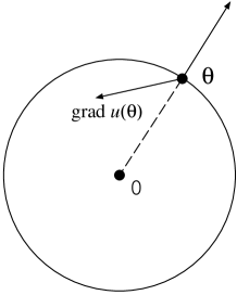
Figure 1: Gradient of $u(\theta)$

This can be seen as follows. Suppose $\|\hat{\theta}_{n}^{*}\|>r$. Let $\tilde{\theta}$ be the maximizer of $u(\theta)$ on the sphere (the boundary of the ball). Then at $\tilde{\theta}$ the gradient of $\nabla u(\tilde{\theta})$ is a positive multiple of $\theta$ and this contradicts $\tilde{\theta}^{\prime}\nabla u(\tilde{\theta})\leq 0$.

As in the previous subsection, using this time the lower bound in (10), we have

$$\theta^{\prime}\nabla u(\theta)\leq\theta^{\prime}{\cal S}_{n}-\theta^{\prime}{\cal V}_{n}\theta e^{-L_{c,n}\|\theta\|}.$$

Now

$$|\theta^{\prime}{\cal S}_{n}|=|\theta^{\prime}{\cal V}_{n}{\cal V}_{n}^{-1}{\cal S}_{n}|\leq\|\theta^{\prime}{\cal V}_{n}\|\cdot\|{\cal V}_{n}^{-1}{\cal S}_{n}\|$$

and

$$\|\theta^{\prime}{\cal V}_{n}\|^{2}=\theta^{\prime}{\cal V}_{n}^{2}\theta\leq\|\theta\|^{2}\lambda_{\max,n}^{2}.$$

Hence

$$|\theta^{\prime}{\cal S}_{n}|\leq\|\theta\|\lambda_{\max,n}\|{\cal V}_{n}^{-1}{\cal S}_{n}\|.$$

Furthermore

$$\theta^{\prime}{\cal V}_{n}\theta e^{-L_{c,n}\|\theta\|}\geq\lambda_{\min,n}\|\theta\|^{2}e^{-L_{c,n}\|\theta\|}.$$

Therefore

$$\theta^{\prime}\nabla u(\theta)\leq\lambda_{\min,n}\|\theta\|\big{(}L_{\lambda,n}\|{\cal V}_{n}^{-1}{\cal S}_{n}\|-\|\theta\|e^{-L_{c,n}\|\theta\|}\big{)}.$$

For $\|\theta\|=3L_{\lambda,n}\|{\cal V}_{n}^{-1}{\cal S}_{n}\|$

$$L_{\lambda,n}\|{\cal V}_{n}^{-1}{\cal S}_{n}\|-\|\theta\|e^{-L_{c,n}\|\theta\|}=L_{\lambda,n}\|{\cal V}_{n}^{-1}{\cal S}_{n}\|(1-3e^{-3L_{c,n}L_{\lambda,n}\|{\cal V}_{n}^{-1}{\cal S}_{n}\|})$$

Then for $\|{\cal V}_{n}^{-1}{\cal S}_{n}\|\leq 1/(3L_{c,n}L_{\lambda,n})$

$$3e^{-3L_{\lambda,n}L_{c,n}\|{\cal V}_{n}^{-1}{\cal S}_{n}\|}\geq 3e^{-1}>1.$$

Hence, if $\|{\cal V}_{n}^{-1}{\cal S}_{n}\|\leq 1/(3L_{c,n}L_{\lambda,n})$, we have $\theta^{\prime}\nabla u(\theta)<0$ for all $\theta$ with $\|\theta\|=3L_{\lambda,n}\|{\cal V}_{n}^{-1}{\cal S}_{n}\|$. By the remark just after Proposition 4.4, this completes the proof of Lemma 4.3.

4.2.2 Behavior of the hindsight strategy

We summarize properties of $\log{\cal K}_{n}^{\hat{\theta}_{n}^{*}}$ in view of the standard theory of exponential families ([2]) in statistical inference. Define

$$\psi_{i}(\theta)=\log(1+p_{i}(e^{\theta c_{i}}-1)),\quad\psi(\theta)=\sum_{i=1}^{n}\psi_{i}(\theta).$$

Note that $\psi_{i}(\theta)$ is the cumulant generating function (potential function) for the logistic regression model, which is an exponential family model with the natural parameter $\theta$. Hence each $\psi_{i}(\theta)$ and $\psi(\theta)$ are convex in $\theta$. Indeed by (9), the Hessian matrix $H_{\psi_{i}}(\theta)$ of $\psi_{i}$ is given as

$$H_{\psi_{i}}(\theta)=c_{i}c_{i}^{\prime}\frac{p_{i}(1-p_{i})e^{\theta^{\prime}c_{i}}}{(1+p_{i}(e^{\theta^{\prime}c_{i}}-1))^{2}},$$

which is non-negative definite. The Hessian matrix

$$H_{\psi}(\theta)=\sum_{i=1}^{n}H_{\psi_{i}}(\theta)$$

of $\psi$ is positive definite if ${\cal V}_{n}$ is positive definite, which is the Fisher information matrix in terms of the natural parameter $\theta$.

Convexity of $\psi_{i}$ implies concavity of $\log{\cal K}_{n}^{\theta}=\theta^{\prime}{\cal T}_{n}-\psi(\theta)$, where

$${\cal T}_{n}=\sum_{i=1}^{n}c_{i}x_{i}={\cal S}_{n}+\sum_{i=1}^{n}c_{i}p_{i}.$$

Hence if the maximum of $\log{\cal K}_{n}^{\theta}$ is attained at a finite value $\hat{\theta}_{n}^{*}$, then the “maximum likelihood estimate” $\hat{\theta}_{n}^{*}$ satisfies “the likelihood equation”

$$\frac{\partial}{\partial\theta}\log{\cal K}_{n}^{\theta}=0$$

or equivalently

$${\cal T}_{n}=\nabla\psi(\hat{\theta}_{n}^{*}).$$ (12)

The likelihood equation can also be written as

$$0=\sum_{i=1}^{n}(x_{i}-\hat{p}_{i}^{*})c_{i},\qquad\hat{p}_{i}^{*}=\hat{p}_{i;n}^{*}=\frac{p_{i}e^{\hat{\theta}_{n}^{*}c_{i}}}{1+p_{i}(e^{\hat{\theta}_{n}^{*}c_{i}}-1)}.$$

From this it follows that $\hat{\theta}_{n}^{*}=0$ if and only if ${\cal T}_{n}=\sum_{i=1}^{n}c_{i}p_{i}$.

Regard (12) as determining $\hat{\theta}_{n}^{*}$ in terms of $t={\cal T}_{n}$, i.e., $\hat{\theta}_{n}^{*}=\hat{\theta}_{n}^{*}(t),t={\cal T}_{n}$. This is the inverse map of $t=\nabla\psi(\theta)$. Differentiating $t=\nabla\psi(\theta)$ again with respect to $\theta$ we obtain the Jacobi matrix

$$J=\frac{\partial t}{\partial\theta}=H_{\psi}(\theta)$$

as the Hessian matrix of $\psi$. Hence the Jacobi matrix $\partial\hat{\theta}_{n}^{*}/\partial{\cal T}_{n}$ is written as

$$\frac{\partial\hat{\theta}_{n}^{*}}{\partial{\cal T}_{n}}=H_{\psi}(\hat{\theta}_{n}^{*}({\cal T}_{n}))^{-1}.$$ (13)

Now $\log{\cal K}_{n}^{\hat{\theta}_{n}^{*}}=\log{\cal K}_{n}^{\hat{\theta}_{n}^{*}({\cal T}_{n})}$ is the Legendre transformation (cf. Chapter 3 of [1]) of $\log{\cal K}_{n}^{\theta}$:

$$\log{\cal K}_{n}^{\hat{\theta}_{n}^{*}(t)}=\hat{\theta}_{n}^{*}(t)^{\prime}t-\psi(\hat{\theta}_{n}^{*}(t)),\qquad t={\cal T}_{n}.$$

Differentiating $\log{\cal K}_{n}^{\hat{\theta}_{n}^{*}(t)}$ with respect to $t$, by (12) we obtain

$$\frac{\partial}{\partial t}\log{\cal K}_{n}^{\hat{\theta}_{n}^{*}(t)}=\hat{\theta}_{n}^{*}(t)+(t-\nabla\psi(\hat{\theta}_{n}^{*}(t))\frac{\partial\hat{\theta}_{n}^{*}}{\partial t}=\hat{\theta}_{n}^{*}(t).$$ (14)

By (13) the Hessian matrix of $\log{\cal K}_{n}^{\hat{\theta}_{n}^{*}(t)}$ is given by $H_{\psi}(\hat{\theta}_{n}^{*}(t))^{-1}$.

We are now ready to prove the following proposition.

Proposition 4.5.

With the same setting as in Lemma 4.3,

$$\|{\cal V}_{n}^{-1}{\cal S}_{n}\|\leq\frac{1}{3L_{c,n}L_{\lambda,n}}\ \ \Rightarrow\ \ e^{-C_{n}\|{\cal V}_{n}^{-1}{\cal S}_{n}\|}\leq\frac{\log{\cal K}_{n}^{\hat{\theta}_{n}^{*}}}{{\cal S}_{n}^{\prime}{\cal V}_{n}{\cal S}_{n}/2}\leq e^{C_{n}\|{\cal V}_{n}^{-1}{\cal S}_{n}\|},$$

where $C_{n}=3L_{c,n}L_{\lambda,n}$.

Proof.

For given ${\cal T}_{n}$, $\bar{\cal T}_{0}=\sum_{i=1}^{n}c_{i}p_{i}$ and for $s\in[0,1]$, consider

$$g(s)=\hat{\theta}_{n}^{*}(\bar{\cal T}_{0}+s{\cal S}_{n})^{\prime}(\bar{\cal T}_{0}+s{\cal S}_{n})-\psi(\hat{\theta}_{n}^{*}(\bar{\cal T}_{0}+s{\cal S}_{n})).$$

Then $\log{\cal K}_{n}^{\hat{\theta}_{n}^{*}({\cal T}_{n})}=g(1)$. It is easily seen that $g(0)=0$. By (14)

$$g^{\prime}(s)=\hat{\theta}_{n}^{*}(\bar{\cal T}_{0}+s{\cal S}_{n})^{\prime}{\cal S}_{n}.$$

Again it is easily seen that $g^{\prime}(0)=0$, since $\hat{\theta}_{n}^{*}(\bar{\cal T}_{0})=0$. Then

$$g(1)=\int_{0}^{1}\int_{0}^{s}g^{\prime\prime}(u)duds.$$

Now

$$g^{\prime\prime}(u)={\cal S}_{n}^{\prime}H_{\psi}(\hat{\theta}_{n}^{*}(\bar{\cal T}_{0}+u{\cal S}_{n}))^{-1}{\cal S}_{n}.$$

By (10)

$$e^{-\|\hat{\theta}_{n}^{*}(\bar{\cal T}_{0}+u{\cal S}_{n})\|L_{c,n}}{\cal S}_{n}^{\prime}{\cal V}_{n}^{-1}{\cal S}_{n} \leq{\cal S}_{n}^{\prime}H_{\psi}(\hat{\theta}_{n}^{*}(\bar{\cal T}_{0}+u{\cal S}_{n}))^{-1}{\cal S}_{n}$$

$$\leq e^{\|\hat{\theta}_{n}^{*}(\bar{\cal T}_{0}+u{\cal S}_{n})\|L_{c,n}}{\cal S}_{n}^{\prime}{\cal V}_{n}^{-1}{\cal S}_{n}.$$

Also $\int_{0}^{1}\int_{0}^{s}1duds=1/2$. Furthermore by Lemma 4.3, if $\|{\cal V}_{n}^{-1}{\cal S}_{n}\|\leq 1/(3L_{c,n}L_{\lambda,n})$ then $\|\hat{\theta}_{n}^{*}(\bar{\cal T}_{0}+u{\cal S}_{n})\|\leq 3L_{\lambda,n}\|{\cal V}_{n}^{-1}{\cal S}_{n}\|$ for all $0\leq u\leq 1$. Combining these results we have the proposition. ∎

As in Proposition 4.5 we have the following corollary.

Corollary 4.6.

In the same setting as in Theorem 4.1 Skeptic can weakly force

$$E_{1}\ \Rightarrow\ \lim_{n}\frac{\log{\cal K}_{n}^{\hat{\theta}_{n}^{*}}}{{\cal S}_{n}^{\prime}{\cal V}_{n}^{-1}{\cal S}_{n}/2}=1.$$

4.2.3 Laplace method for evaluating the difference of the hindsight strategy and the logistic strategy

In the last subsection we clarified the behavior of the capital process for the hindsight strategy. Now we employ the standard Laplace method to evaluate the difference of the hindsight strategy and the logistic strategy (Section 5 of [3], Chapter 3.1 of [8]).

Lemma 4.7.

Let $\pi$ be a prior density supporting a neighborhood of the origin and let ${\cal K}_{n}^{\pi}$ denote its capital process. For $\xi\in E_{1}$ such that $\lim_{n}{\cal V}_{n}^{-1}{\cal S}_{n}=0$,

$$\lim_{n}\frac{\log{\cal K}_{n}^{\hat{\theta}_{n}^{*}}-\log{\cal K}_{n}^{\pi}}{(1/2)\log\det{\cal V}_{n}}=0.$$ (15)

Proof.

For $\theta$ close to the origin, expanding $\log{\cal K}_{n}^{\theta}$ around $\hat{\theta}_{n}^{*}$ we have

$$\log{\cal K}_{n}^{\theta}=\log{\cal K}_{n}^{\hat{\theta}_{n}^{*}}-\frac{1}{2}(\theta-\hat{\theta}_{n}^{*})^{\prime}H_{\psi}(\tilde{\theta}_{n})(\theta-\hat{\theta}_{n}^{*}),$$

where $\tilde{\theta}_{n}$ is on the line segment joining $\theta$ and $\hat{\theta}_{n}^{*}$. Hence

$${\cal K}_{n}^{\theta}={\cal K}_{n}^{\hat{\theta}_{n}^{*}}\times\exp(-\frac{1}{2}(\theta-\hat{\theta}_{n}^{*})^{\prime}H_{\psi}(\tilde{\theta}_{n})(\theta-\hat{\theta}_{n}^{*})).$$

Now by the standard Laplace method we obtain (15). ∎

Finally we give a proof of Theorem 4.2.

Proof of Theorem 4.2.

By Corollary 4.6 and Lemma 4.7

$$\log{\cal K}_{n}^{\pi}=\frac{1}{2}\log\det{\cal V}_{n}\;\big{(}\frac{{\cal S}_{n}^{\prime}{\cal V}_{n}^{-1}{\cal S}_{n}}{\log\det{\cal V}_{n}}-1+o(1)\big{)}.$$

Hence if $\limsup_{n}{\cal S}_{n}^{\prime}{\cal V}_{n}^{-1}{\cal S}_{n}/\log\det{\cal V}_{n}>1$, then $\limsup_{n}\log{\cal K}_{n}^{\pi}=\infty$. ∎

4.3 Monotonicity with respect to the forecast probability

Here we consider the case that $\log(p_{n}/(1-p_{n}))$ itself is an element of the vector of the side information $c_{n}$ and hence is multiplied by a coefficient in (5). For notational convenience we here eliminate $\log(p_{n}/(1-p_{n}))$ from $c_{n}$ and write (5) as

$$\log\frac{\hat{p}_{n}}{1-\hat{p}_{n}}=\beta\log\frac{p_{n}}{1-p_{n}}+\tau_{n},$$ (16)

where $\tau_{n}$ denotes the effect of side information other than $\log(p_{n}/(1-p_{n}))$. Intuitively $\beta$ represents how much trust Skeptic puts in Forecaster. If $\beta=0$ then Skeptic entirely ignores Forecaster’s $p_{n}$ and if $\beta=1$ then Skeptic takes $p_{n}$ for granted. The value of $\beta\in(0,1)$ corresponds to partial trust in $p_{n}$. It is somewhat surprising to see that $\beta>1$ in the case of probability of precipitation announced by the Japan Meteorological Agency in Section 5.2.

We now investigate how $\nu_{n}$ in (2) behaves with respect to $p_{n}$ for given $p_{1},c_{1},x_{1},\dots,p_{n-1},c_{n-1},\allowbreak x_{n-1}$. This is an important question from the viewpoint of defensive forecasting ([20], [18]), because in defensive forecasting we want to obtain $p_{n}$ for which $\nu_{n}=0$. For notational simplicity we now omit the subscript $n$ and write (6) as

$$\hat{p}=\frac{p\left(\frac{p}{1-p}\right)^{\beta-1}e^{\tau}}{1+p\left(\frac{p}{1-p}\right)^{\beta-1}e^{\tau}}.$$

Then

$$\nu(p)=\frac{\hat{p}-p}{p(1-p)}=\frac{p^{\beta-1}e^{\tau}-(1-p)^{\beta-1}}{p^{\beta}e^{\tau}+(1-p)^{\beta}}.$$

Differentiating this with respect to $p$ we obtain

$$\frac{d\nu(p)}{dp}=\frac{-e^{2\tau}p^{2(\beta-1)}+e^{\tau}p^{\beta-2}(1-p)^{\beta-2}(\beta-2+2p(1-p))-(1-p)^{2\beta-2}}{(p^{\beta}e^{\tau}+(1-p)^{\beta})^{2}}.$$

The numerator of $d\nu(p)/dp$ can be written as

$$-(e^{\tau}p^{\beta-1}-(1-p)^{\beta-1})^{2}+e^{\tau}(\beta-1)p^{\beta-2}(1-p)^{\beta-2},$$

which is non-positive for $\beta\leq 1$. Hence we have the following proposition.

Proposition 4.8.

Under the logistic regression model (16), for $\beta\leq 1$ the betting ratio $\nu_{n}(p_{n})$ is monotone decreasing in $p_{n}$.

It is natural that $\nu_{n}$ is monotone decreasing in $p_{n}$, because if $p_{n}$ is too high and Skeptic does not believe it, then Skeptic will bet on the non-occurrence $x_{n}=0$.

For the special case of $\beta=1$,

$$\nu_{n}(p_{n})=\frac{e^{\tau_{n}}-1}{1+p_{n}(e^{\tau_{n}}-1)},$$

which is bounded and monotone in $p_{n}\in[0,1]$. For $\beta<1$, $\nu_{n}(p_{n})$ is unbounded and it can be easily seen that

$$\lim_{p_{n}\downarrow 0}\frac{\nu_{n}(p_{n})}{1/p_{n}}=1,\qquad\lim_{p_{n}\uparrow 1}\frac{\nu_{n}(p_{n})}{1/(1-p_{n})}=-1.$$

We can interpret the first limit as follows. Suppose that $p_{n}=1/1000$, i.e. the price of a ticket is 1/1000 of a dollar. In this case Skeptic can buy $1000$ tickets with one dollar and has the chance of winning $1000$ dollars. Hence Skeptic may want to buy $1000$ tickets. Thus it is reasonable that $\nu$ and $p_{n}$ are inversely proportional when $p_{n}$ is small.

5 Experiments

In this section we give some numerical studies of our strategy. In Section 5.1 we present some simulation results and in Section 5.2 we apply our strategy against probability forecasting by the Japan Meteorological Agency.

5.1 Some simulation studies

We consider three cases and apply three strategies to these examples. In our simulation studies Reality chooses her moves probabilistically, either by Bernoulli trials or by a Markov chain model.

• Case 1: $x_{n}$ is a Bernoulli variable with the success probability 0.7 and $p_{n}$ alternates between $0.4$ and $0.6$ (i.e. $0.4=p_{1}=p_{3}=\cdots$ and $0.6=p_{2}=p_{4}=\cdots$).

• Case 2: $x_{n}$ is a Bernoulli variable with the success probability 0.5 and $p_{n}$ alternates between $0.4$ and $0.6$.

• Case 3: $p_{n}=0.5$ and $x_{n}$ is generated by a Markov chain model with transition probabilities shown in Figure 2.

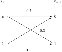
Figure 2: Transition probabilities for $x_{n}$

• Strategy 1: $\theta$ is a scalar and $c_{n}=1$ in (5). Assume that the prior density for $\theta$ is given as uniform distribution for [0,1]. The capital process is written as

  $${\cal K}_{n}^{\pi}=\int_{0}^{1}\frac{e^{\theta\sum_{i=1}^{n}x_{i}}}{\prod_{i=1}^{n}(1+p_{i}(e^{\theta}-1))}d\theta.$$

• Strategy 2: $\theta^{\prime}=[\theta_{1},\beta-1]$ and $c_{n}^{\prime}=[1,\log\frac{p_{n}}{1-p_{n}}]$. Assume independent priors for $\theta_{1}$ and $\beta$, which are uniform distributions over [0,1]. The capital process is written as

  $${\cal K}_{n}^{\pi}=\int_{0}^{1}\int_{0}^{1}\frac{e^{\theta_{1}\sum_{i=1}^{n}x_{i}+(\beta-1)\sum_{i=1}^{n}x_{i}\log\frac{p_{i}}{1-p_{i}}}}{\prod_{i=1}^{n}(1+p_{i}(e^{\theta_{1}+(\beta-1)\log\frac{p_{i}}{1-p_{i}}}-1))}d\theta_{1}d\beta.$$

• Strategy 3: $\theta^{\prime}=[\theta_{1},\beta-1,\theta_{3}]$ and $c_{n}^{\prime}=[1,\log\frac{p_{n}}{1-p_{n}},x_{n-1}]$. Assume independent priors for $\theta_{1}$, $\beta$ and $\theta_{3}$, which are uniform distributions over [0,1]. The capital process is written as

  $${\cal K}_{n}^{\pi}=\int_{0}^{1}\int_{0}^{1}\int_{0}^{1}\frac{e^{\theta_{1}\sum_{i=1}^{n}x_{i}+(\beta-1)\sum_{i=1}^{n}x_{i}\log\frac{p_{i}}{1-p_{i}}+\theta_{3}\sum_{i=1}^{n}x_{i}x_{i-1}}}{\prod_{i=1}^{n}(1+p_{i}(e^{\theta_{1}+(\beta-1)\log\frac{p_{i}}{1-p_{i}}+\theta_{3}x_{i-1}}-1))}d\theta_{1}d\beta d\theta_{3}.$$

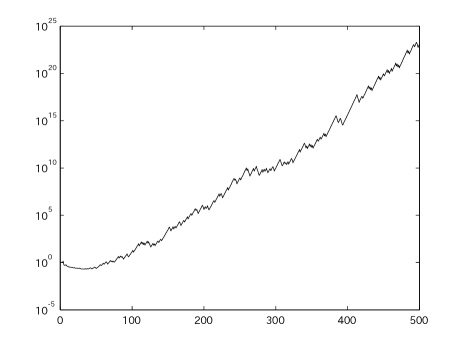
Figure 3: Case 1 with strategy 1

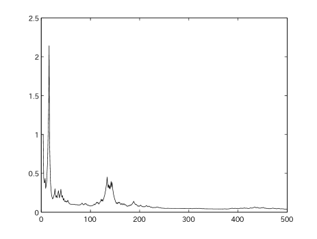
Figure 4: Case 2 with strategy 1

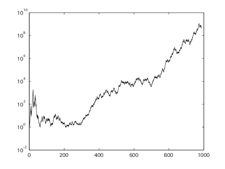
Figure 5: Case 2 with strategy 2

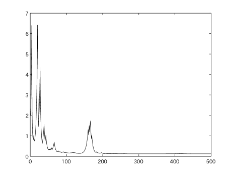
Figure 6: Case 3 with strategy 2

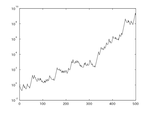
Figure 7: Case 3 with strategy 3

As shown in Figure 4 and Figure 4, we can beat Reality by strategy 1 only in case 1. So we improve our strategy and apply strategy 2 to case 2. We can see from Figure 6 and Figure 6 that strategy 2 can work well in case 2 but still not effective in case 3. Finally, we use strategy 3 in case 3 and observe that it shows a good result for Skeptic in Figure 7.

From these simulations, we see that Skeptic can beat Reality with more flexible strategy utilizing more side information.

5.2 Betting against probability of precipitation by the Japan Meteorological Agency

Now we apply our strategy to probability of precipitation provided by the Japan Meteorological Agency. We collected the forecast probabilities for the Tokyo area from archives of the morning edition of the Mainichi Daily News and the actual weather data on 9:00 and 15:00 of each day for Tokyo area from http://www.weather-eye.com/ for the period of three years from January 1, 2009 to December 31, 2011. We counted a day as rainy if the data on this site records rain on 9:00 or on 15:00 of that day in Tokyo area.

The forecast probability $p_{n}$ is only announced as multiples of 10% (i.e. $0\%,10\%,\dots,90\%,\allowbreak 100\%$) by JMA. The data are summarized in Table 1. $p_{n}$ represents the probability of precipitation on day $n$ and $x_{n}$ indicates the actual precipitation. Actual ratio is calculated from the ratio of the number of rainy days to all days for a given value of $p_{n}$.

Table 1: Actual ratio of rainy days

$p_{n}$(%)	$x_{n}=1$	$x_{n}=0$	Actual Ratio(%)
0	1	61	1.6
10	10	324	3.0
20	24	193	11.1
30	36	117	23.5
40	20	26	43.5
50	67	56	54.5
60	38	14	73.1
70	36	7	85.7
80	36	4	90.0
90	22	1	95.6
100	3	0	100

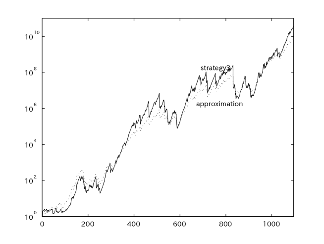
Figure 8: Beating JMA by strategy 3 with $\beta$ uniform over $[0,2]$

The distinct feature of the prediction by JMA is that that $p_{n}$ tends to be closer to 50% than the actual ratio. For example, when JMA announces $p_{n}=20\%$, the actual ratio is only $11.1\%$. Similarly when JMA announces $p_{n}=80\%$, the actual ratio is $90\%$. Hence JMA has the tendency of avoiding clear-cut forecasts.

In the hindsight strategy, the value of $\beta$, which is a coefficient for $\log(p_{n}/(1-p_{n}))$ in strategy 3 is close to 1.5. Hence we modified strategy 3 of the previous section, so that the prior for $\beta$ is uniform between 0 and 2. We also substituted $p_{n}=1\%$ and $p_{n}=99\%$ for $p_{n}=0\%$ and $p_{n}=100\%$, respectively, because our strategy is not defined for $p_{n}=0\%$ or $100\%$. Figure 8 shows the behavior of strategy 3 and the approximation ${\cal S}_{n}^{\prime}{\cal V}_{n}^{-1}{\cal S}_{n}/2$. We see that our strategy works very well against JMA by exploiting its tendency of avoiding clear-cut forecasts. It is also of interest that the capital process shows a seasonal fluctuation and it does not perform well for the rainy season (June and July) in Tokyo area.

6 Summary and discussion

In this paper we proposed a Bayesian logistic betting strategy in the binary probability forecasting game with side information (BPFSI). We proved some theoretical results and showed good performance of our strategy against probability forecasting by Japanese Meteorological Agency.

Here we discuss some topics for further investigation.

We considered implications of a single Bayesian logistic betting strategy in BPFSI. We can also take a look at the sequential optimizing strategy (SOS) of [11] in BPFSI. Under the condition $\hat{\theta}_{n}^{*}\rightarrow 0$, Bayesian strategy and SOS should behave in the same way. However we could not succeed to prove weak forcing of $\hat{\theta}_{n}^{*}\rightarrow 0$ by SOS alone.

For the case of $d=1$ we could employ approaches of [14] to prove results similar to Theorem 4.2. In [14] we also discussed Reality’s strategies. It is of interest to study strategies of Forecaster or Reality in the binary probability forecasting game with side information. Defensive forecasting ([20], [18]) can be considered as a strategy of Forecaster.

We extended the binary probability forecasting game by including side information. In our formulation side information $c_{n}$ is announced by Forecaster and in our logistic betting strategy $c_{n}$ is used as regressors in a logistic regression. However Skeptic can use any transformation of $c_{n}$ in his strategy. In this sense, it might be more natural to formulate the game, where $c_{n}$ is announced by Skeptic. Binary probability forecasting game is often considered from the viewpoint of prequential probability ([7]) and leads to the notion of randomness of the sequence $p_{1}x_{1}p_{2}x_{2}\dots$ ([19], [13]). From the viewpoint of prequential probability it might also be natural to consider side information $c_{n}$ as a part of moves by Skeptic for testing the randomness of $p_{1}x_{1}p_{2}x_{2}\dots$.

We assumed multidimensional $c_{n}$. However from the viewpoint of game-theoretic probability, we do not lose much generality by restricting $c_{n}$ to be a scalar, since if Skeptic can weakly force events $E_{1},\dots,E_{d}$ then he can weakly force $E_{1}\cap\dots\cap E_{d}$. By the same reasoning we can also consider $d=\infty$, because if Skeptic can weakly force $E_{1},E_{2},\dots,$ then he can weakly force $\cap_{i=1}^{\infty}E_{i}$. Interpretation and formulation of side information in game-theoretic probability needs further investigation.

References

- [1] V. I. Arnol′d. Mathematical Methods of Classical Mechanics, volume 60 of Graduate Texts in Mathematics. Springer-Verlag, New York, second edition, 1989. Translated from the Russian by K. Vogtmann and A. Weinstein.
- [2] O. Barndorff-Nielsen. Information and Exponential Families. John Wiley & Sons Inc., New York, 1978. Wiley Series in Probability and Mathematical Statistics.
- [3] T. M. Cover. Universal portfolios. Math. Finance, 1(1):1–29, 1991.
- [4] T. M. Cover and E. Ordentlich. Universal portfolios with side information. IEEE Trans. Inform. Theory, 42(2):348–363, 1996.
- [5] T. M. Cover and J. A. Thomas. Elements of Information Theory. Wiley, Hoboken, NJ, second edition, 2006.
- [6] A. P. Dawid. Probability forecasting. In Encyclopedia of Statistical Sciences, volume 7, pages 210–218. Wiley, New York, 1986.
- [7] A. P. Dawid and V. G. Vovk. Prequential probability: principles and properties. Bernoulli, 5(1):125–162, 1999.
- [8] J. L. Jensen. Saddlepoint Approximations. Oxford University Press, Oxford, 1995.
- [9] J. L. Kelly, Jr. A new interpretation of information rate. Bell. System Tech. J., 35:917–926, 1956.
- [10] M. Kumon, A. Takemura, and K. Takeuchi. Capital process and optimality properties of a Bayesian skeptic in coin-tossing games. Stoch. Anal. Appl., 26(6):1161–1180, 2008.
- [11] M. Kumon, A. Takemura, and K. Takeuchi. Sequential optimizing strategy in multi-dimensional bounded forecasting games. Stochastic Process. Appl., 121:155–183, 2011.
- [12] L. C. MacLean, E. O. Thorp, and W. T. Ziemba. The Kelly Capital Growth Investment Criterion: Theory and Practice. World Scientific handbook in financial economic series. World Scientific, 2011.
- [13] K. Miyabe. An optimal superfarthingale and its convergence over a computable topological space, 2011. To appear in Proceedings of Solomonoff 85th Memorial Conference at Melbourne, Australia.
- [14] K. Miyabe and A. Takemura. Convergence of random series and the rate of convergence of the strong law of large numbers in game-theoretic probability. Stochastic Process. Appl., 122(1):1–30, 2012.
- [15] G. Shafer, A. Shen, N. Vereshchagin, and V. Vovk. Test martingales, Bayes factors and -values. Statist. Sci., 26(1):84–101, 2011.
- [16] G. Shafer and V. Vovk. Probability and Finance: It’s Only a Game! Wiley, 2001.
- [17] K. Takeuchi, A. Takemura, and M. Kumon. New procedures for testing whether stock price processes are martingales. Computational Economics, 37(1):67–88, 2010.
- [18] V. Vovk, I. Nouretdinov, A. Takemura, and G. Shafer. Defensive forecasting for linear protocols. In H. S.Jain and E.Tomita, editors, Proceedings of the 16th international conference on algorithmic learning theory, number 3734 in LNAI, pages 459–473, 2005.
- [19] V. Vovk and A. Shen. Prequential randomness and probability. Theoret. Comput. Sci., 411(29-30):2632–2646, 2010.
- [20] V. Vovk, A. Takemura, and G. Shafer. Defensive Forecasting. In R.G.Cowell and Z.Ghahramani, editors, Proceedings of the tenth international workshop on artificial intelligence and statistics, pages 365–372, 2005.