Crossing the Gould Belt in the Orion vicinity ^,

Abstract

Context. The recent star formation history in the solar vicinity is not yet well constrained, and the real nature of the so-called Gould Belt is still unclear.

Aims. We present a study of the large-scale spatial distribution of 6482 ROSAT All-Sky Survey (RASS) X-ray sources in approximately 5000 deg² in the general direction of Orion. We examine the astrophysical properties of a sub-sample of $\sim 100$ optical counterparts, using optical spectroscopy. This sub-sample is then used to investigate the space density of the RASS young star candidates by comparing X-ray number counts with Galactic model predictions.

Methods. The young star candidates were selected from the RASS using X-ray criteria. We characterize the observed sub-sample in terms of spectral type, lithium content, radial and rotational velocities, as well as iron abundance. A population synthesis model is then applied to analyze the stellar content of the RASS in the studied area.

Results. We find that stars associated with the Orion star-forming region, as expected, do show a high lithium content. As in previous RASS studies, a population of late-type stars with lithium equivalent widths larger than Pleiades stars of the same spectral type (hence younger than $\sim 70-100$ Myr) is found widely spread over the studied area. Two new young stellar aggregates, namely “X-ray Clump 0534+22” (age $\sim 2-10$ Myr) and “X-ray Clump 0430$-$08” (age $\sim 2-20$ Myr), are also identified.

Conclusions. The spectroscopic follow-up and comparison with Galactic model predictions reveal that the X-ray selected stellar population in the general direction of Orion is characterized by three distinct components, namely the clustered, the young dispersed, and the widespread field populations. The clustered population is mainly associated with regions of recent or ongoing star formation and correlates spatially with molecular clouds. The dispersed young population follows a broad lane apparently coinciding spatially with the Gould Belt, while the widespread population consists primarily of active field stars older than 100 Myr. We expect the still “bi-dimensional” picture emerging from this study to grow in depth as soon as the distance and the kinematics of the studied sources will become available from the future Gaia mission.

1 Introduction

If the global scenario of the star formation history (SFH) of the Milky Way is still not fully outlined (see Wyse 2009 for a review), the recent SFH in the solar neighborhood is far from being constrained. In particular, the recent local star formation rate is poorly known because of the difficulty encountered in properly selecting young late-type stars in large sky areas from optical data alone (Guillout et al. 2009). This situation has improved thanks to wide-field X-ray observations, such as the ROSAT All-Sky Survey (RASS), which allowed for efficiently detection of young, coronally active stars in the solar vicinity (Guillout et al. 1999). Nearby star-forming regions (SFRs) have been searched for pre-main sequence (PMS) stars, and many new nearby moving groups and widely-spread young low-mass stars have been identified over the past decades based on the RASS data (Feigelson & Montmerle 1999; Zuckerman & Song 2004; Torres et al. 2008; Guillout et al. 2009, and references therein).

It has been suggested that at least some of these widely-spread young stars might be associated with the so-called Gould Belt (GB; Guillout et al. 1998), a disk-like structure made up of gas, young stars, and OB associations (see, e.g., Lindblad 2000; Elias et al. 2009). However, the existence of such structure and its possible origin remain somewhat controversial (Sánchez et al. 2007, and references therein). Also, it is unclear whether its putative young stellar population is in excess with respect to predictions of Galactic models, which would indicate a recent episode of star formation. On the other hand, there is no evidence of molecular material within $\sim$100 pc that can explain the origin of the distributed young stars as in situ star formation. Such young stars may thus represent a secondary star formation event in clouds that condensed from the ancient Lindblad ring supershell, or may have been formed in recent bursts of star formation from already disrupted and evaporated small clouds (see Bally 2008, and references therein).

An accurate census of the young population in different star-forming environments and the comparison between observations and predictions from Galactic models are thus required in order to constrain the low-mass star formation in the solar vicinity.

In this work, we revisit the results by Walter et al. (2000) on the large-scale spatial distribution of 6482 RASS X-ray sources in a 5000 deg² field centered on the Orion SFR, and use optical, low and high resolution, spectroscopic observations to investigate the optical counterparts to 91 RASS sources (listed in Table Crossing the Gould Belt in the Orion vicinity ^,) distributed on a sky “strip” perpendicular to the Galactic Plane, in the general direction of Orion. The complete sky coverage of the RASS allows us to perform an unbiased analysis of the spatial distribution of X-ray active stars. Our main goal is to characterize spectroscopically the optical counterparts of the X-ray sources and compare their space density with predictions of Galactic models.

In Sect. 2 we define the sky areas and describe the selection of young X-ray emitting star candidates; in Sect. 3 we present the spectroscopic observations; in Sect. 4 we characterize the young optical counterparts in terms of spectral type, lithium detection, H$\alpha$ line, radial/rotational velocity and iron abundance; in Sect. 5 we compare the spatial distribution of the young X-ray emitting star candidates with expectations from Galactic models; in Sect. 6 we discuss the results and draw our conclusions.

2 Selection of study areas and X-Ray sources

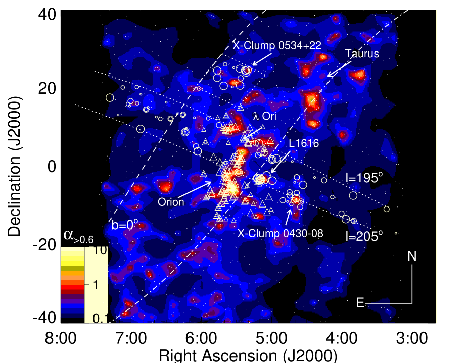
Figure 12: Large-scale spatial distribution of 1483 candidate young stars (small dots) in the Orion and Taurus-Auriga associations. The X-ray sources have been selected from the ROSAT All-Sky Survey. Their space density is color-coded, where the parameter $\alpha$ represents the discriminant probability; the higher $\alpha$ the more probable is the occurrence of a source corresponding to a young star. Circles refer to sources observed spectroscopically in this work, while triangles represent targets previously analyzed by Alcalá et al. (1996) and Alcalá et al. (2000). The symbol size increases with the lithium equivalent width $EW$ (0, $<$150, 150–300, $>$300 mÅ). The dashed line coincides with the position of the Galactic Plane, while the dash-dotted line represents the Gould Belt, as given by Guillout et al. (1998). The sky strip ($195{\degr}<l_{II}<205{\degr}$, $-60{\degr}<b_{II}<15{\degr}$) selected by us across the Gould Belt in the Orion vicinity is also shown together with the area selected on the X-Clump 0534+22 (see Sect. 4). The regions of enhanced density of young star candidates and of high-lithium stars southward of the Galactic Plane coincide with the location of the Gould Belt midplane. North is up and East to the left.

Our analysis is based on the method introduced by Sterzik et al. (1995) for selecting young star candidates from the RASS sources using the X-ray hardness ratios and the ratio of X-ray to optical flux. Fig. 12 is a revisited version of Fig. 3 by Walter et al. (2000), showing the color-coded space density of the RASS sources based on the $\alpha$ parameter, which is related to the probability of a source to be a young X-ray emitting star. Following the Sterzik et al. (1995) selection criteria, X-ray sources with $\alpha>0.6$ are most likely young stars with a positive rate of 80%. In the figure we recognize: $i)$ the surface density enhancements corresponding to 1483 young candidates, distributed over an area much larger than the molecular gas; $ii)$ space density enhancements not necessarily associated with previously known regions of active (or recent) star formation (e.g., at $\alpha=5^{\rm h}34^{\rm m}$, $\delta=+22{\degr}01^{\prime}$ and at $\alpha=4^{\rm h}30^{\rm m}$, $\delta=-08{\degr}$); the local enhancement at $\alpha=5^{\rm h}07^{\rm m}$ and $\delta=-03{\degr}20^{\prime}$ corresponds to the L1616 cometary cloud (Alcalá et al. 2004; Gandolfi et al. 2008); $iii)$ a broad lane apparently connecting Orion and Taurus, which extends further southeastward; this wide and contiguous structure is not symmetric about the Galactic plane, but rather seems to follow the GB as drawn by Guillout et al. (1998); $iv)$ the surface density of young star candidates drops down to a background value of about 0.1 candidate star/deg² near $b_{II}=0{\degr}$, or below that value at higher Galactic latitudes.

2

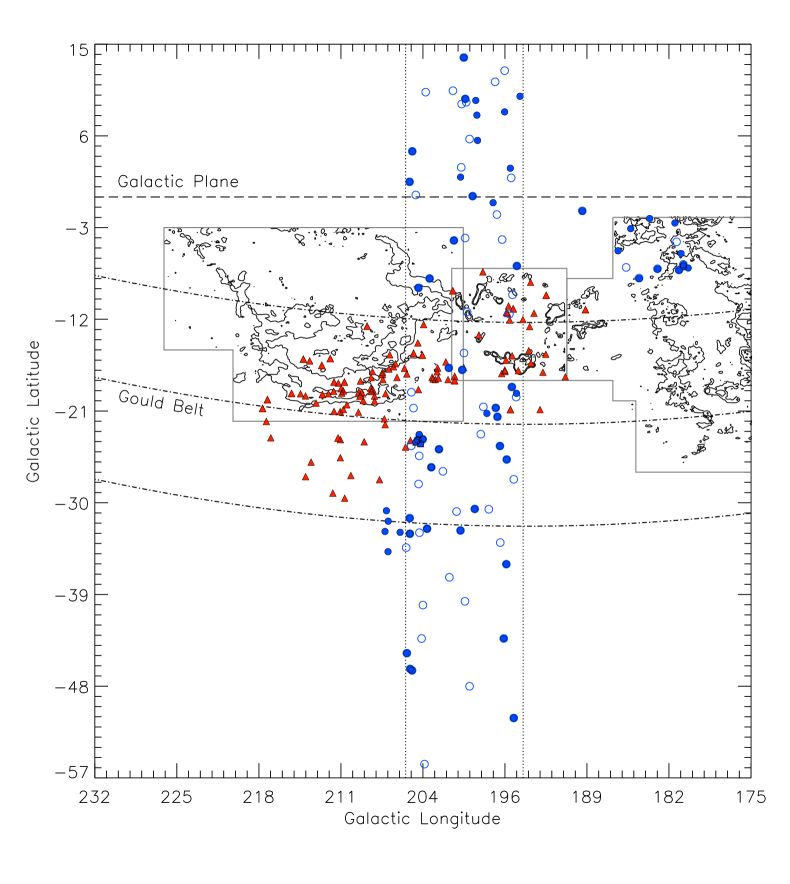
Figure 1: Large-scale spatial distribution of our targets (circles) and those of Alcalá et al. (1996, 2000; triangles). Empty symbols refer to low-resolution spectra, while filled symbols represent objects observed at high resolution. The dotted lines mark the strip, the long-dashed line is the Galactic Plane, while the dash-dotted lines represent the Gould Belt disk, as outlined by Guillout et al. (1998). The CO J=1$\rightarrow$0 emission contour maps by Dame et al. (2001) of the Orion, Monoceros, and Taurus Molecular Clouds, and the $\lambda$ Orionis H ii region are also overlaid.

In order to study the global properties of the different populations close to the Orion SFR, we selected a $10{\degr}\times 75{\degr}$ strip (see Fig. 12) perpendicular to the Galactic Plane (hence presumably crossing the GB), and in the Orion vicinity. Inside this $\sim 750$ deg² strip ($l_{II}^{\rm min}=195{\degr}$, $l_{II}^{\rm max}=205{\degr}$, $b_{II}^{\rm min}=-60{\degr}$, $b_{II}^{\rm max}=15{\degr}$), 806 RASS X-ray sources were detected with a high confidence level by the Standard Analysis Software System (SASS; Voges 1992). According to the Sterzik et al. (1995) selection criteria, 198 of these sources are young star candidates. Additionally, we selected a region of $10{\degr}\times 10{\degr}$ (see Fig. 12) centered at $\alpha=5^{\rm h}34^{\rm m}$ and $\delta=+22{\degr}01^{\prime}$, where a density enhancement of young star candidates is present. We call this previously unrecognized enhancement “X-ray Clump 0534+22” (hereafter, X-Clump 0534+22). Analogously, we also identify as “X-ray Clump 0430$-$08” (hereafter, X-Clump 0430$-$08) the unknown density enhancement at $\alpha=4^{\rm h}30^{\rm m}$ and $\delta=-08{\degr}$. Although the X-Clump 0534+22 almost coincides in direction with the Crab nebula, it is physically unrelated to the supernova remnant.

3 Spectroscopic observations and data reduction

We conducted a spectroscopic follow-up of 91 young stellar candidates inside the strip and clump regions. Table 1 gives a summary of the spectroscopic observations, while the full list of the observed stars is reported in Table Crossing the Gould Belt in the Orion vicinity ^,). Throughout the paper, we term as ‘young star’ an optical counterpart that shows characteristics typical of weak-lined T-Tauri stars, i.e. weak H$\alpha$ emission ($EW_{\rm H\alpha}\raisebox{-2.15277pt}{$\>\stackrel{{\scriptstyle\textstyle<}}{{\sim}}\>$}10$ Å) and strong lithium absorption.

3.1 Low-resolution spectroscopy

Low-resolution spectroscopic observations were carried out during 25-30 November 1995 and 16-21 December 1996 using the Boller & Chivens (B&Ch) Cassegrain spectrographs attached to the 1.5m telescope of the European Southern Observatory (ESO, Chile) and to the 2.1m of the Observatorio Astronómico Nacional de San Pedro Mártir (OAN-SPM, México), respectively. Table 1 gives information on the instrumental setups and number of observed objects. The spectral resolution was verified by measuring the full width at half maximum of several lines in calibration spectra. The spectra were reduced following the standard procedure of MIDAS software packages using the same procedure described in Alcalá et al. (1996).

Table 1: Summary of the spectroscopic observations.

Telescope	Instrument	Range	Resolution	#
		(Å)	($\lambda/\Delta\lambda$)	stars
1.5m@ESO	B&Ch	3400–6800	1 600	66
2.1m@OAN-SPM	B&Ch	3600–9900	1 500	6
2.2m@CAHA	FOCES	4200–7000	30 000	61

Note: 30 stars were observed only at low resolution, and 20 only at high resolution. One star was observed at low resolution with both the B&Ch spectrographs.

About sixty of the 198 strip sources plus fourteen stars in the X-Clump 0534+22 direction were investigated spectroscopically at low resolution (see Table Crossing the Gould Belt in the Orion vicinity ^, and Fig. 1). The observational strategy consisted in covering the whole range of right ascension and declination each night in order to avoid any bias in the resulting spatial distribution of the young star candidates. The spatially unbiased sample so far observed and characterized spectroscopically by us is therefore incomplete, representing $\sim$40% of the total sample of potential young X-ray emitting candidates. Yet, it can be used to study the strength of the lithium absorption line within the RASS young stellar sample as a function of Galactic latitude, and to trace the young stellar population in the general direction of Orion.

3.2 High-resolution spectroscopy

High-resolution spectroscopic observations were conducted in several runs in the period between October 1996 and December 1998, using the Fiber Optics Cassegrain Échelle Spectrograph (FOCES) attached to the 2.2m telescope at the Calar Alto Observatory (CAHA, Spain). Some seventy spectral orders are included in these spectra covering the range from 4200 to 7000 Å, with a nominal mean resolving power of $\lambda/\Delta\lambda\approx$30 000 (see Table 1). The reduction was performed using IDL routines specifically developed for this instrument (Pfeiffer et al. 1998). Details on the data reduction are given in Alcalá et al. (2000).

We also retrieved FEROS spectra for two stars of our sample (namely, 2MASS J03494386$-$1353108 and 2MASS J04354055$-$1017293) from the ESO Science Archive. The FEROS spectra extend between 3600 Å and 9200 Å with a resolving power $R$=48 000 (Kaufer et al. 1999). The data were reduced using a modified version of the FEROS-DRS pipeline (running under the ESO-MIDAS context FEROS) which yields a wavelength-calibrated, merged, normalized spectrum, following the steps specified in Desidera et al. (2001).

In summary, high-resolution spectroscopy exists for 61 stars, 33 inside inside the strip, 13 in the X-Clump 0534+22, 8 associated with the high space-density X-Clump 0430$-$08 (see in Fig. 12 the spatial distribution at $\alpha=4^{\rm h}30^{\rm m}$ and $\delta=-08{\degr}$), and 7 inside the strip associated to the L1616 clump. The high-resolution sample thus represents $\sim$70% of the known lithium stars in the strip, and can be used to verify the reliability of the lithium strength obtained from the low-resolution spectra.

In order to increase the statistics, we also include in our analysis the on-strip lithium-rich stars identified by Alcalá et al. (1996) and Alcalá et al. (2000), which were observed with the same instruments, set-ups, and observational strategy.

4 Characterization of the selected young X-ray counterparts

4.1 Near-IR color-color diagram

We identified all our targets in the Two Micron Sky Survey (2MASS) catalogue. In Table Crossing the Gould Belt in the Orion vicinity ^, we list both the RASS Bright Source Catalogue (Voges et al. 1999) and 2MASS designations, as well as an alternative name. The stellar coordinates are those from the 2MASS catalogue. We then examined the properties of the sources in the $JHK$ bands using their 2MASS magnitudes (Cutri et al. 2003) looking for eventual color excess. The $(J-H)$ versus $(H-K)$ diagram (Fig. 2) shows that our sample mostly consists of stars without near-IR excess, with the only exception of 2MASS J05122053$-$0255523=V531 Ori, which was classified as a classical T Tauri star by Gandolfi et al. (2008). All stars follow the MS branch with a spread mostly ascribable to photometric uncertainties. Only 2MASS J04405981$-$0840023 departs from the sequence, maybe due to its double-lined binary nature (Covino et al. 2001).

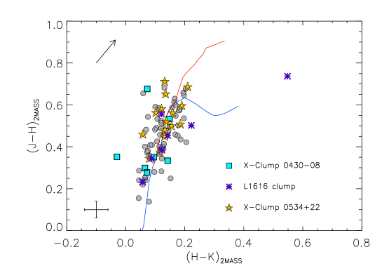
Figure 2: 2MASS $(J-H)$ versus $(H-K)$ diagram for the observed sources. Squares, asterisks, and stars represent objects in the three clumps, as indicated in the legend. The circles refer to the “non-clump” stars. The solid curve shows the relation between these indexes for main sequence stars (lower branch; Bessell & Brett 1988) and giants (upper branch; Kenyon & Hartmann 1995), where the 2MASS color trasformations were used. The $A_{\rm V}=1$ mag reddening vector is shown with an arrow. The typical 2MASS photometric errors are overplotted on the lower-left corner of the panel.

4.2 Spectral types, lithium detection, and H$\alpha$ equivalent width

Spectral types were determined from the low-resolution spectra by comparison with a grid of bright spectral standard stars (from F0 to M5) observed with the same dispersion and instrumental set-up in each observing run. The methods described in Alcalá et al. (1995) were used for the classification, leading to an accuracy of about $\pm 1$ sub-class in most cases. The spectral types are reported in Table Crossing the Gould Belt in the Orion vicinity ^,, while their distribution is plotted in Fig. 3. The sample is composed of late-type stars with a distribution peaked around G9–K1.

Figure 3: Spectral type distribution of the young stellar candidates.

In our low-resolution spectroscopic follow-up, the Orion stars fall basically in four categories (see Table Crossing the Gould Belt in the Orion vicinity ^,): $i)$ stars with weak H$\alpha$ emission ($-3$ Å$\raisebox{-2.15277pt}{$\>\stackrel{{\scriptstyle\textstyle<}}{{\sim}}\>$}EW_{\rm H\alpha}\raisebox{-2.15277pt}{$\>\stackrel{{\scriptstyle\textstyle<}}{{\sim}}\>$}0$ Å) and Li absorption (21 stars); $ii)$ stars with H$\alpha$ filled-in or in absorption and Li absorption (40 stars); $iii)$ stars with H$\alpha$ in emission but no Li absorption (8 stars); and $iv)$ stars with H$\alpha$ in absorption but no Li detection (4 stars). In total, 61 stars with clear lithium detections were found throughout the strip, as well as in the clumps. Practically all lithium stars have spectral types ranging from late F to K7/M0 peaking around G9 (see Table Crossing the Gould Belt in the Orion vicinity ^,). The effective temperature versus spectral type relation for dwarfs by Kenyon & Hartmann (1995) was used to estimate the $\log T_{\rm eff}$ values listed in Table Crossing the Gould Belt in the Orion vicinity ^,.

At this point, it is important to stress that: $i)$ at the Orion distance, our sample is limited to masses $>0.8M_{\odot}$ (Alcalá et al. 1998) because of the RASS flux limit; $ii)$ the Li equivalent width ($EW_{\rm Li}$) may be overestimated in low-resolution spectra because of blending mainly with the nearby Fe i line at $\lambda=6707.4$ Å (see Sect. 4.3). The latter issue can be overcome by using high-resolution spectroscopy (see Sections 3.2 and 4.3).

4.3 Lithium strength: low- versus high-resolution measurements

For 43 stars we obtained both low- and high-resolution spectra. Based on these data, we estimated that the mean lithium equivalent width measured on low-resolution spectra ($EW_{\rm Li}^{\rm lr}$) is overestimated by $\sim$20 mÅ, with a standard deviation of $\pm 60$ mÅ on the average difference between the low and high resolution measurements. Interestingly, for several stars, the $EW_{\rm Li}^{\rm lr}$ matches well with the lithium equivalent width obtained from high-resolution spectra ($EW_{\rm Li}^{\rm hr}$) and, in some cases, $EW_{\rm Li}^{\rm lr}$ values are underestimated (see Table Crossing the Gould Belt in the Orion vicinity ^,). The good match between the $EW_{\rm Li}^{\rm lr}$ and $EW_{\rm Li}^{\rm hr}$ values is due to the fact that the lithium strength of these stars is indeed high and also to the experience we gathered on measuring $EW_{\rm Li}$ in low-resolution spectra.

In Fig. 4 (left panel), the lithium equivalent widths of the 47 stars in our sample and the 38 from Alcalá et al. (1996), observed at low-resolution and falling inside the strip, are plotted versus the logarithm of the effective temperature, for the following three bins of Galactic latitude: $i)$ $-20{\degr}<b_{II}<-10{\degr}$, coinciding with the Orion Complex, $ii)$ $-30{\degr}<b_{II}<-20{\degr}$, corresponding approximately to the position of the Gould Belt at those Galactic longitudes, and $iii)$ in the two ranges $-10{\degr}<b_{II}<15{\degr}$ and $-60{\degr}<b_{II}<-30{\degr}$ (directions that we consider as likely dominated by field stars). Similar plots were produced for the stars observed at high resolution (see right panel of Fig. 4). The upper envelope for the Pleiades stars, adapted from the Soderblom et al. (1993) data, is also overplotted. In both panels, a spatial segregation of lithium strength can be observed, thus justifying the use of both high- and low-resolution $EW_{\rm Li}$. Practically all the stars located on the Orion region fall above the Pleiades upper envelope, as expected. The majority of these stars are indeed very young. Note that many stars, located in the region of the hypothetical Gould Belt, also have strong lithium absorption but tend to be closer to the Pleiades upper envelope. Finally, the majority of the lithium field stars fall closer to/or below the Pleiades upper envelope, and most of them seem to have an age similar to the Pleiades or older. Nevertheless, a few of these field stars have lithium strengths comparable to those of stars in Orion or the Gould Belt direction, and seem to be also very young.

4.3.1 Lithium abundance

The lithium abundance ($\log n{\rm(Li)}$) was derived from the $EW_{\rm Li}^{\rm hr}$ and $T_{\rm eff}$ values and using the non-LTE curves-of-growth reported by Pavlenko & Magazzù (1996), assuming $\log g=4.5$. The main source of error in $\log n{\rm(Li)}$ is the uncertainty in $T_{\rm eff}$, which is about $\Delta T_{\rm eff}=150$ K. Taking this value and a mean error of about 10 mÅ in $EW_{\rm Li}$ into account, we estimate a mean $\log n{\rm(Li)}$ error ranging from $\sim$0.22 dex for cool stars ($T_{\rm eff}\approx 3700$ K) down to $\sim$0.13 dex for warm stars ($T_{\rm eff}\approx 5800$ K). Moreover, the assumption of $\log g=4.5$ affects the lithium abundance determination, in the sense that the lower the surface gravity the higher the lithium abundance. In particular, the difference in $\log n{\rm(Li)}$ may rise to $\sim$0.1 dex, when considering stars with mean values of $EW_{\rm Li}=300$ mÅ and $T_{\rm eff}=5000$ K and assuming $\Delta\log g=1.0$ dex. Hence, this means that our assumption of $\log g=4.5$ would eventually lead to underestimate the lithium abundance.

In Fig. 5 (left panel), we show the lithium abundance as a function of the effective temperature for the stars on the strip, but coded in three bins of Galactic latitude, hence, according to their spatial location with respect to the Orion SFR and the Gould Belt. We also overplot the isochrones of lithium burning as calculated by D’Antona & Mazzitelli (1997). Three groups of stars can be identified according to the lithium content and spatial location. First, stars showing high-lithium content with ages even younger than $\sim 2-5\times 10^{6}$ yr, mostly located on/or close to the Orion clouds; second, stars with lithium content consistent with ages $\sim 5\times 10^{6}-1\times 10^{7}$ yr, supposedly distributed on the Gould Belt, and third, stars with lithium indicating a wide range of ages, but located far off the Orion SFR or the GB.

In Fig. 5 (right panel), we show the same plot, but for the three identified young aggregates, respectively represented by three different symbols. The lithium content in the X-Clump 0430$-$08 corresponds to an age of about $2\times 10^{6}-2\times 10^{7}$ yr, while for the L1616 group it indicates an age of $2-7\times 10^{6}$ yr, consistent with the Alcalá et al. (2004) and Gandolfi et al. (2008) findings. Finally, the lithium content of the stars in X-Clump 0534+22 indicates a relatively narrow age range of $2-10$ Myr, which is consistent with the age inferred from the HR diagram when adopting a distance of 140 pc (see Sect. 5.2).

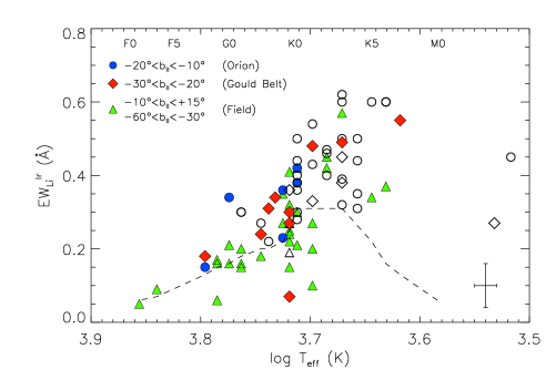
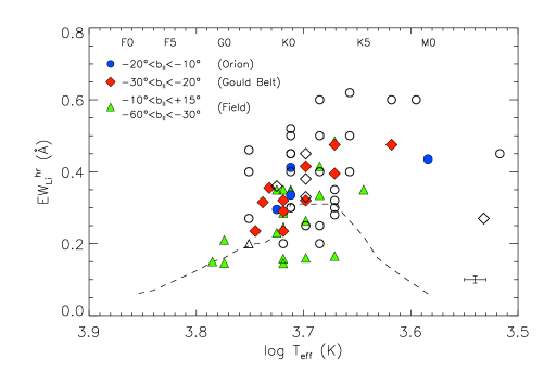
Figure 4: Lithium ($\lambda$6707.8 Å) equivalent width versus $\log T_{\rm eff}$ for the stars in the strip ($195\degr<l_{II}<205\degr$), observed at low (left panel) and high (right panel) resolution. Three different bins of Galactic latitude were considered (see also Fig. 1). The upper envelope for the Pleiades sample, as adapted from Soderblom et al. (1993), is overplotted as a dashed line. Mean errors in $EW_{\rm Li}^{\rm lr}$ ($\sim$60 mÅ), $EW_{\rm Li}^{\rm hr}$ ($\sim$10 mÅ), and $\log T_{\rm eff}$ ($\sim$100 K, as obtained from the spectral synthesis) are overplotted on the lower-right corner of each panel. Open symbols represent the Alcalá et al. (1996) and Alcalá et al. (2000) results from low (left panel) and high (right panel) resolution spectra, respectively.

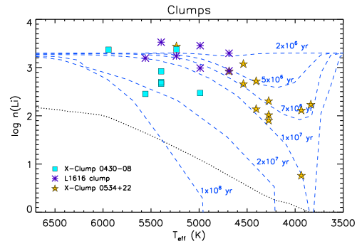
Figure 5: Lithium abundance versus effective temperature for stars observed at high resolution (filled symbols refer to our sample, while open symbols represent the Alcalá et al. (2000) measurements). The “lithium isochrones” by D’Antona & Mazzitelli (1997) in the $2\times 10^{6}-1\times 10^{8}$ yr range are overlaid with dashed lines. Dotted lines represent the limiting detectable $\log n{\rm(Li)}$, as derived from Pavlenko & Magazzù (1996) non-LTE curves-of-growth, assuming 10 mÅ as mean $EW_{\rm Li}$ error and adding quadratically the mean contribution of the iron line at 6707.4 Å computed from the empirical relation obtained by Soderblom et al. (1993) between $B-V$ color and $EW_{\rm Fe}$ (Kenyon & Hartmann 1995 tables were used to convert $B-V$ colors into $T_{\rm eff}$). Left panel: Stars located along the strip crossing the GB in the range $195\degr<l_{II}<205\degr$ (see Fig. 1) and three bins of Galactic latitude. Right panel: Stars in known (L1616) and unknown (X-Clump 0430$-$08 and X-Clump 0534+22) groups.

4.3.2 Rotational and radial velocity measurements

Stellar rotation may affect internal mixing, hence lithium depletion. A large spread in rotation rates may introduce a spread in lithium abundance, which is observed in young clusters (Balachandran et al. 2011, and references therein). In order to investigate such Li behaviour in the stars of our sample, rotational ($v\sin i$) velocities were derived by using the same cross-correlation method as described in Alcalá et al. (2000).

In Fig. 6 (left panel) we show the lithium abundance versus $v\sin i$ for the on-strip stars, coded with three different symbols, indicating their spatial location as defined in the previous Section. Despite the low statistics, the typical $\log n{\rm(Li)}-v\sin i$ behaviour observed in young clusters, i.e. a larger spread in $\log n{\rm(Li)}$ for lower $v\sin i$ values, is apparent for the stars projected in Orion and in the Gould Belt. In order to assign a confidence level to this trend, a one-side $2\times 2$ Fisher’s exact test was performed (Agresti 1992). For the test, we adopt 30 km s^-1 and 2.0 dex as dividing limits in $v\sin i$ and $\log n{\rm(Li)}$, respectively. We find a $p$-value of 0.54 as chance that random data would yield the trend, indicating a probability of correlation of 46%. Hence, the low-number statistics prevents a rigorous demostration of the apparent trend shown in the plots. More measurements of $\log n{\rm(Li)}$ and $v\sin i$ for stars projected in Orion and the Gould Belt are needed to firmly establish the preservation of Li content at high $v\sin i$ ($\raisebox{-2.15277pt}{$\>\stackrel{{\scriptstyle\textstyle>}}{{\sim}}\>$}25$ km s^-1) values. The above $\log n{\rm(Li)}-v\sin i$ behaviour is even less evident, however, for the stars flagged as “field”. These stars show a spread in $\log n{\rm(Li)}$ at all $v\sin i$ values. The difference between the three stellar groups is supported by the different dispersion in the $\log n{\rm(Li)}-v\sin i$ diagram (see left-bottom panel of Fig. 6).

In Fig. 6 (right panel) the lithium abundance is plotted as a function of $v\sin i$ for the stars in the young aggregates. Similar conclusions can be achieved as for the young stars projected in Orion and the Gould Belt. The $\log n{\rm(Li)}-v\sin i$ behaviour in the X-Clump 0534+22 aggregate is enhanced by the star with the lowest lithium abundance and low $v\sin i$. This star, namely 2MASS J06020094+1955290, shows basically the same activity level as the other targets (see $EW_{\rm H\alpha}$ in Table Crossing the Gould Belt in the Orion vicinity ^, and $\log\frac{f_{X}}{f_{V}}$ values in the histograms of the top panel of Fig. 10) and is indistinguishable from the other stars in the aggregate.

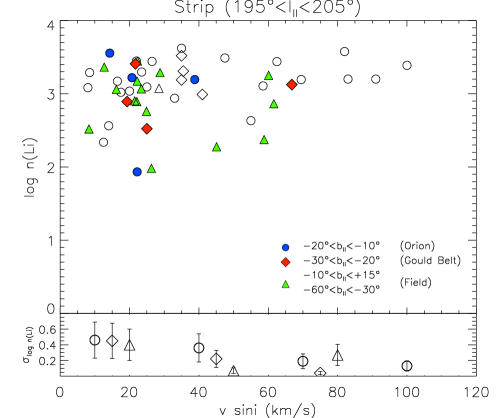
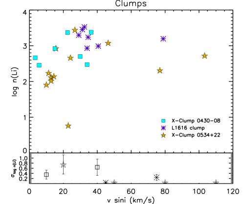
Figure 6: Lithium abundance versus $v\sin i$ for stars observed at high resolution. Symbols as in Fig. 5. Bottom panels show for each group the $\log n{\rm(Li)}$ dispersion as a function of $v\sin i$ at the following bins: $0-30$, $30-60$, $60-90$, $90-120$ km s^-1. The values are shifted in $v\sin i$ to better visualize the symbols.

Stellar radial velocities (RV) were also measured by means of cross-correlation analysis. In Fig. 7 (left panel) we show the distribution of RV for the on-strip stars, also divided in three bins of Galactic latitude as above. While the field stars show a wide RV range, the RV distribution of the stars projected on Orion and the GB is peaked at values of $\sim$18 km s^-1, i.e. close to the tail at low RV of the Orion sub-associations (from 19.7$\pm$1.7 km s^-1 for 25 Ori to $24.87\pm 2.74$ km s^-1 for the ONC, to $\sim$30.1$\pm$1.9 km s^-1 for OB1b; see, Briceño et al. 2007; Biazzo et al. 2009) or to the Taurus-Auriga distribution (16.03$\pm$6.43 km s^-1; Bertout & Genova 2006).

In Fig. 7 (right panel) the RV distribution of the stars in the young aggregates is shown. With the exception of two stars in the X-Clump 0430$-$08, likely spectroscopic binaries, the RV of these groups is in the range 10–35 km s^-1, fairly consistent with Orion or Taurus. It is worth mentioning that the RV distribution of widely distributed young stars in Orion shows a double peak (Alcalá et al. 2000), which can be explained as due to objects associated with different kinematical groups, likely located at different distances.

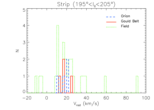
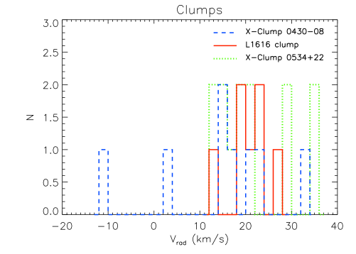
Figure 7: Radial velocity distribution for the on-strip stars (left panel) and in the young aggregates (right panel), respectively.

4.3.3 Iron abundance

Metallicity measurements were obtained following the prescriptions by Biazzo et al. (2011a, b) and the 2010 version of the MOOG code (Sneden 1973).

After a screening of the sample for the selection of suitable stars (G0-K7 stars with $v\sin i\raisebox{-2.15277pt}{$\>\stackrel{{\scriptstyle\textstyle<}}{{\sim}}\>$}20$ km s^-1 and no evidence of multiplicity), a total of 11 stars in our sample, plus 8 stars from Alcalá et al. (2000) were analyzed for iron abundance measurements. In Table 2 we list the final results, together with effective temperature, surface gravity, and microturbulence (the number of lines used is also given in Columns 6 and 8). An initial temperature value was set using the ARES automatic code (Sousa et al. 2007); initial microturbulence was set to $\xi=1.5$ km s^-1, and initial gravity to $\log g=4.0$. The effective temperatures derived using this method and from spectral types (Sect. 4.2) agree within $\sim$200 K (i.e. $\sim$1.5 spectral sub-class) on the average. For the stars observed with both FOCES and FEROS spectrographs, the values of the stellar parameters are in close agreement. It is worth noticing that the target 2MASS J05214684+2400444 was also analyzed by Santos et al. (2008; their 1RXSJ052146.7), who derived stellar parameters ($T_{\rm eff}=4921\pm 59$ K, $\log g=4.05\pm 0.29$, $\xi=1.92\pm 0.07$ km s^-1, $v\sin i=13$ km s^-1) and iron abundance ([Fe/H]$=-0.07\pm 0.07$) in good agreement with our determinations, thus excluding any significant systematic error due to different datasets (see Biazzo et al. 2011b).

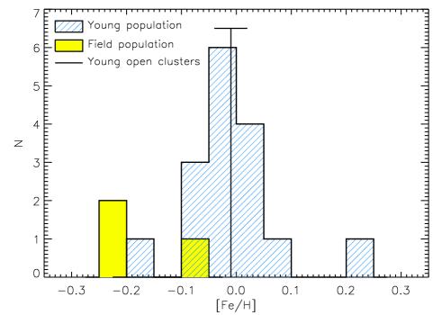
Figure 8: [Fe/H] distribution for stars observed with the FOCES spectrograph and representing the young population (dashed histogram) and the field population (filled histogram). The bar represents the mean value of [Fe/H]=$-0.01\pm 0.03$ obtained for open clusters younger than 150 Myr within 500 pc from the Sun (see Biazzo et al. 2011a, and references therein).

In Figs. 8 and 13 we show the distribution of iron abundance for the stars with strong lithium absorption (16 stars representing the young population) and those without (3 stars representing the old field population). Two results are noticeable: $i)$ the stars with high lithium content show a distribution with a mean [Fe/H]$=-0.02\pm 0.09$, consistent with the value of $-0.01\pm 0.03$ for open clusters younger than 150 Myr and within 500 pc from the Sun (see Biazzo et al. 2011a for details); $ii)$ stars with no lithium absorption line show [Fe/H] values which are within the metallicity distribution of field stars in the solar neighborhood ([Fe/H]=$-0.10\pm 0.24$; Santos et al. 2008). This would imply that the young stars in the Orion vicinity have solar metallicity, consistent with the distribution of the Galactic thin disk in the solar neighborhood (Biazzo et al. 2011b).

Table 2: Spectroscopic stellar parameters and iron abundance derived with MOOG for low-rotating stars observed at high resolution.

Star	$T_{\rm eff}$	$\log g$	$\xi$	[Fe i/H]∗	# lines	[Fe ii/H]∗∗	# lines
	(K)	(dex)	(km/s)	(dex)		(dex)
X-Clump 0534+22
2MASS J05263833+2231546	4750	4.4	2.0	$-0.08\pm 0.15$	43	$-0.08\pm 0.15$	3
2MASS J05263826+2231434	4750	4.0	1.9	$-0.07\pm 0.12$	42	$-0.06\pm 0.11$	5
2MASS J05214684+2400444	5000	4.3	2.2	$-0.04\pm 0.11$	44	$-0.02\pm 0.06$	4
X-Clump 0430$-$08
2MASS J04431640$-$0937052	6000	4.6	1.4	$+0.22\pm 0.08$	66	$+0.22\pm 0.10$	9
”	6050	4.6	1.4	+0.26$\pm$0.08	78	+0.22$\pm$0.10	9
2MASS J04443859$-$0724378	5900	4.4	1.5	$+0.03\pm 0.09$	64	$+0.03\pm 0.08$	11
Strip
2MASS J03494386$-$1353108	5400	4.5	1.4	$+0.00\pm 0.09$	64	$-0.01\pm 0.12$	9
”	5500	4.6	1.6	+0.05$\pm$0.09	70	+0.03$\pm$0.13	10
2MASS J05274490+0313161	5000	4.3	1.7	$-0.02\pm 0.17$	51	$-0.01\pm 0.23$	3
2MASS J06134773+0846022	5050	3.6	1.6	$-0.25\pm 0.13$	59	$-0.24\pm 0.13$	9
2MASS J06203205+1331125	5350	4.4	0.3	$-0.23\pm 0.17$	44	$-0.24\pm 0.25$	4
2MASS J06350191+1211359	6100	4.3	1.5	$+0.01\pm 0.13$	45	$+0.00\pm 0.19$	9
2MASS J06513955+1828080	5100	4.7	1.5	$-0.07\pm 0.09$	60	$-0.07\pm 0.13$	5
Alcalá et al. (2000) Sample
RX J0515.6$-$0930	5650	4.5	2.3	$-0.04\pm 0.12$	41	$-0.06\pm 0.23$	4
RX J0517.9$-$0708	5100	4.2	1.8	$+0.06\pm 0.13$	47	$+0.05\pm 0.14$	4
RX J0531.6$-$0326	5250	4.3	1.7	$-0.02\pm 0.09$	53	$-0.03\pm 0.08$	5
RX J0538.9$-$0624	5550	4.4	1.3	$+0.01\pm 0.11$	58	$+0.02\pm 0.20$	10
RX J0518.3+0829	5300	4.2	2.0	$-0.04\pm 0.11$	21	$-0.02\pm 0.15$	3
RX J0510.1$-$0427	4950	4.6	1.9	$-0.10\pm 0.12$	34	$-0.00\pm 0.24$	2
RX J0520.0+0612	4750	4.1	2.2	$-0.17\pm 0.12$	45	$-0.17\pm 0.30$	5
RX J0520.5+0616	4900	4.1	2.4	$-0.08\pm 0.17$	29	$-0.07\pm 0.04$	3

Note: The two stars observed with FEROS are indicated in italics.
^∗ The iron abundances are relative to the Sun. Adopting $T_{\rm eff}^{\odot}=5770$ K, $\log g^{\odot}=4.44$, and $\xi^{\odot}=1.1$ km s^-1, we obtain $\log n^{\odot}{\rm({Fe\textsc{i}})}=7.53\pm 0.04$ and $\log n^{\odot}{\rm({Fe\textsc{ii}})}=7.53\pm 0.06$ from a FOCES spectrum, and $\log n^{\odot}{\rm({Fe\textsc{i}})}=7.50\pm 0.05$ and $\log n^{\odot}{\rm({Fe\textsc{ii}})}=7.50\pm 0.06$ from a FEROS spectrum.
^∗∗ The listed errors are the internal ones in $EW$, represented by the standard deviation on the mean abundance determined from all lines. The other source of internal error includes uncertainties in stellar parameters (Biazzo et al. 2011a). Taking into account typical errors in $T_{\rm eff}$ ($\sim$70 K), $\log g$ ($\sim$0.2 dex), and $\xi$ ($\sim$0.2 dex), we derive an error of $\sim$0.05 dex in [Fe/H] due to uncertainties on stellar parameters.

5 Discussion

5.1 RASS and Galactic Models

How many young, X-ray active stars are actually expected inside the strip? A comparison of the number counts with predictions from Galactic models provides the basis for a quantitative analysis of source excesses (or deficits) in order to understand their origin. Because of the strong dependence of stellar X-ray emission on age, an X-ray view of the sky preferentially reveals young stars (ages $\leq 100$ Myr), in contrast to optical star counts which only loosely constrain the stellar population for ages $\leq 10^{9}$ yr. A Galactic X-ray star count modeling starts adopting a Galactic model, including assumptions about the spatial and temporal evolution of the star formation rate and the initial mass function, and uses characteristic X-ray luminosity functions attributed to the different stellar populations. Such models are able to predict the number of stars per square degree $N(>S)$ with X-ray flux $>S$, taking into account the dependence on Galactic latitude, spectral type, and stellar age. An elaborate Galactic model, including kinematics, is the evolution synthesis population model developed at Besançon (Robin & Crézé 1986), which computes the density and the distribution of stars as a function of the observing direction, age, spectral type, and distance. Our X-ray synthetic model is based on the Besançon optical model and has been first applied to the analysis of the RASS stellar population by Guillout et al. (1996). Motch et al. (1997) successfully used this model in a low Galactic latitude RASS area in Cygnus and found a good agreement between observations and predicted number counts using the ‘canonical’ assumption of a uniform and continuous star formation history in the solar vicinity. We note however that, following the publication of Hipparcos results, the stellar density in the solar neighborhood was revised (lowered) in the Besançon model thus propagating in the X-ray population model predictions. The apparent disagreement between observed and predicted number count (by $\sim$20%) can in fact be explained by the population of old close binaries (RS CVn-like systems), as suggested by Favata et al. (1988) and Sciortino et al. (1995). RS CVn systems for which the high magnetic activity level results from the synchronization of rotational and orbital periods can mimic young active stars and contaminate the young star population detected in soft X-ray survey (Frasca et al. 2006; Guillout et al. 2009). The eight stars with H$\alpha$ emission, but no Li absorption identified by us (c.f. Section 4.2) may represent this type of objects.

Figure 9: Cumulative $\log N(>S)-\log S$ distributions for RASS data in the Orion vicinity. A field centered on the Galactic Plane is shown with a dotted line. The dashed line includes Orion and a section of the Gould Belt. The solid line corresponds to the prediction of our X-ray models at $l_{II}=200\degr$ and zero Galactic latitude. The RASS completeness limit of 0.03 cnts/sec is marked with the double arrow.

In Fig. 9, we compare the RASS stellar counterparts (taken from the Guide Star Catalogue) in our field with the current X-ray Galactic model predictions using a cumulative distribution function $\log N(>S)-\log S$. We select two fields: one centered on the Galactic Plane ($b_{II}=0\degr\pm 10\degr$, $190\degr<l_{II}<220\degr$), and the other, southern, includes Orion and a section of the Gould Belt ($b_{II}=-20\degr\pm 10\degr$, $190\degr<l_{II}<220\degr$). The deviation from a power-law function for both data distributions at a count rate of $\approx$0.03 cnts/sec is related to the completeness limit of the RASS at this value. Comparing these two distributions, it is noticeable how the source density in the area containing Orion exceeds that of the Galactic Plane by about 30$-$60% (at the largest count rates even by a factor of two). Considering that the population of old active binaries is not yet taken into account in our X-ray model, the predictions are in close agreement with the RASS data around the Galactic Plane and with optical counterparts from the Guide Star Catalogue. For the Galactic Plane, this model predicts a surface density of 0.37 stars/deg² at the RASS completeness limit (see Table 3). The source excess in the Orion field can be attributed to the presence of additional, probably younger, X-ray active stars due to recent, more localized star formation which is not included in the Galactic model. In fact, the difference in surface density between the regions in Orion + Gould Belt and the Gould Belt alone is 0.14$\pm$0.04 stars/deg² for the RASS stellar counterparts and of 0.21$\pm$0.07 stars/deg² for the stars with lithium detection, i.e. a significant number of young stars in the general direction of Orion, not necesarily originated in the star formation complex, is evident (see Table 3, where the errors were computed from Poisson statistics). We note that our results are not influenced by the density of active stars: from our spectroscopic identifications, we observed 61 stars in the strip out of 198 young star candidates resulting from the Sterzik et al. (1995) selection criteria. Eight are likely active stars because of their H$\alpha$ emission but no Li detection (see Sect. 4.2). Therefore, inside the 750 deg² strip area, we estimate a surface density of only 0.03 stars/deg² as due to active stars.

Encouraged by the success of our X-ray star count modeling in reproducing the background counts and in revealing the excess of sources associated with Orion, we then performed a more detailed analysis of the RASS sources located in the strip shown in Fig. 12, including the available information on spectroscopic identification and lithium abundance. Our goal is to intercompare average source densities of RASS-selected young stars and to constrain the age distributions in different parts of the strip. Therefore, we divided the strip in three subareas, one is a 200 deg² large field centered on the Galactic Plane and with $-10\degr<b_{II}<+10\degr$, the adjacent 100 deg² area between $-20\degr<b_{II}<-10\degr$ contains the northern parts of the Orion Complex, and the third 100 deg² area between $-30\degr<b_{II}<-20\degr$ is formally unrelated to the Orion molecular clouds but contains a significant part of the Gould Belt in that direction.

In Fig. 10 we compare the number of RASS sources which have stellar counterparts from the Guide Star Catalogue and count rates $\geq 0.03$ cnts/sec (as indicated by the thin-lined histogram) with the numbers of such sources predicted by the Galactic model (indicated by star symbols with statistical error bars). The histograms show the X-ray to optical flux ratio distributions. The thick-lined histogram indicates the RASS sources that have been selected as young star candidates according to the Sterzik et al. (1995) criteria. A subsample of those (hatched histogram) were observed spectroscopically and classified according to lithium absorption strength. The dark grey histogram denotes objects where lithium absorption has been found, and the solid histogram refers to high-lithium stars. We note that the ‘identified’ subsample is by now only complete to 40$-$70% depending on the area. We can draw the following main conclusions:

1. The total number and the flux ratio distribution of the RASS sources are in good agreement with the Galactic model for the Galactic Plane field. High-lithium sources represent about 1/3 of the observed sources. Extrapolating to all RASS-selected young star candidates, we expect a total of about 15 high-lithium sources in this 200 deg² large Galactic Plane field. The Besançon model predicts 72 X-ray sources with ages lower than 150 Myr in this area. The high-lithium sources are expected to be the youngest within our sample, and we can roughly estimate their characteristic age to be around 15/72 $\cdot$ 150 Myr=30 Myr (assuming continuous star formation). This age is consistent with their spectroscopic signature.

2. A large RASS source excess ($\sim$ 100%) is present in the Orion field. The fraction of high-lithium stars among identified sources is now around 9/10. In this 100 deg² field, we expect to find a total of 38 high-lithium stars once all young candidates have been observed.

3. A large RASS source excess (50%) is also present in the field that includes the Gould Belt, preferentially at flux ratios $\log\frac{f_{X}}{f_{V}}>-2$. The fraction of high-lithium stars among observed sources is about 2/3. We expect eventually to find a total of about 17 high-lithium stars in the RASS-selected subsample.

These extrapolations to the total number of expected high-lithium sources should be reliable enough, since the spectroscopic identifications were done on statistically representative subsamples of RASS-selected young star candidates. It is also possible that some of the high-lithium stars present among RASS sources have been missed by the Sterzik et al. (1995) selection criteria. Hence, the extrapolated number of high-lithium X-ray sources in the respective areas is a lower limit.

The results of this Section are summarized in Table 3, where we report the estimated surface density of RASS sources and of high-lithium RASS-selected sources in the three investigated sky areas. While the Galactic Plane source densities are in good agreement with the Galactic X-ray star count model, the source density excesses in the other two directions indicate the presence of additional populations of high-lithium stars younger than 150 Myr.

Table 3: Surface densities (in stars/deg²) of the RASS sources and high-lithium stars compared with the densities as predicted by the X-ray Galactic model for the appropriate Galactic latitude.

	Galactic Plane	Orion+Gould Belt	Gould Belt
RASS ($>$0.03cnts/sec)	0.43$\pm$0.02	0.76$\pm$0.03	0.62$\pm$0.02
Besançon Galactic model	0.37	0.37	0.31
Lithium sources	0.14$\pm$0.02	0.39$\pm$0.06	0.18$\pm$0.04

Figure 10: Detailed comparison of three fields in the strip perpendicular to the Galactic Plane between $l_{II}=195\degr$ and $l_{II}=205\degr$, as shown in Fig. 2. The three areas include: the Galactic Plane, the Orion SFRs, and the Gould Belt, respectively. Histograms are cumulative, not stacked, i.e., each histogram includes the stars in all subcategory histograms.

5.2 The X-ray clumps 0534+22 and 0430$-$08: two new young stellar aggregates?

These two groupings were first recognized as surface density enhancements of X-ray emitting young star candidates (see Fig. 12), and then classified as young star clumps based on the spectroscopic follow-up. In particular, from lithium abundance measurements, the stars in the X-Clump 0534+22 have an age of $\sim 5-10$ Myr, while those in the X-Clump 0430$-$08 of $\sim 2-20$ Myr. Inspection of recent CO maps (see Fig. 1) seems to indicate that the stars in the X-Clump 0534+22 follow the spatial location of some of the Taurus-Auriga dark nebulae (namely L1545, L1548, and L1549; Kenyon et al. 2008). Thus, the X-Clump 0534+22 might be an extension of the Taurus-Auriga association towards the Galactic Plane, alghough the average RV ($\sim 22\pm 8$ km s^-1) of this clump is higher than the mean RV for Taurus, but within the quoted uncertainty. Therefore, it deserves further kinematic studies. We attempt to estimate the stellar luminosities of the X-Clump 0534+22 stars by assuming the distance to Taurus ($d\sim 140$ pc; Kenyon et al. 1994), and adopting the Tycho magnitudes ($V_{\rm Tycho}$; Egret et al. 1992), a solar bolometric magnitude of $M^{\sun}_{\rm bol}=4.64$ (Cox 2000), and the temperatures listed in Table Crossing the Gould Belt in the Orion vicinity ^,. The resulting HR diagram is shown in Fig. 11. The error in $\log L/L_{\sun}$ is estimated considering an uncertainty of 0.1 mag in $V_{\rm Tycho}$. The range of ages $\sim 3-30$ Myr for the stars in the X-Clump 0534+22 appears consistent with the estimates from the lithium abundance (see Fig. 5). Adopting instead the Orion distance ($\sim 400$ pc; Bally 2008) would place the stars close to/or above the birthline in the HR diagram, in contrast with their lithium content and lack of IR excess.

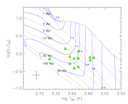
Figure 11: HR diagram for the stars in the X-Clump 0534+22. The pre-main sequence evolutionary tracks of Palla & Stahler (1999), together with their isochrones and birthline are shown by solid, dotted, and dash-dotted lines, respectively. Labels indicating the track masses and the isochronal ages (from 1 to 100 Myr) are also overlaid.

5.3 The variety of populations in the Orion vicinity

Based on the morphology and surface density distribution of the X-ray selected young star candidates, the spectroscopic analysis, and the comparison of RASS number counts with Galactic model predictions, we argue that the analyzed widespread stellar sample consists of a mixture of three distinct populations:

1. The clustered population comprises the dense regions ($\raisebox{-2.15277pt}{$\>\stackrel{{\scriptstyle\textstyle>}}{{\sim}}\>$}5-10$ stars/deg²) associated with sites of active or recent star formation (e.g., OB1a, OB1b, OB1c, $\lambda$ Ori, L1616). These clusters contain the highest fraction of lithium-rich stars. The number counts result considerably in excess when compared to the Galactic model predictions. The stars in these clusters are, on average, among the youngest in our sample and their small spatial dispersion allows us to locate their birthplace. The RASS limit in X-ray luminosity at $M\sim 0.8M_{\odot}$ is $\sim\log L_{\rm X}=30.5$ erg/s; as a consequence, with some caution, we can extrapolate the X-ray luminosity function of RASS sources to lower luminosities (e.g., $\sim 29$ erg/s), and estimate the total number of X-ray emitting young stars in the Orion Complex to be of the order of a few thousand.

2. The broad lane apparently connecting the Orion and Taurus SFRs might contain late-type Gould Belt members and/or stars belonging to large star halos around Orion and/or Taurus, possibly originated from an earlier episode of star formation. We call this component the dispersed young population (density of $\sim 0.5-5$ stars/deg²). This population appears unrelated to any molecular cloud. The number counts in these areas are in significant excess as compared to Galactic model expectations. A high fraction of these sources have strong lithium absorption features rather typical of stars with age $\>\stackrel{{\scriptstyle\textstyle<}}{{\sim}}\>$ 20 Myr. They also show an iron abundance distribution consistent with that of nearby open clusters and associations younger than 150 Myr. Recent analysis including parallax information from Hipparcos and Tycho suggests that these stars are uniformly distributed along the line of sight, as in the disk-like structure proposed by Guillout et al. (1998) for the GB, rather than piling up at the supposed outer edge of the Gould Belt (Bally 2008). On the other hand, the interpretation of large star halos around Orion and/or Taurus as result of an earlier episode of star formation, say about 20 Myr ago, would require an initial velocity dispersion of nearly 10 km/s to explain the extension of such halos, whereas the value typically observed for young associations is less than about 2 km/s, although some authors claim in situ star formation in turbulent cloudlets (Feigelson 1995).

3. The uniformly distributed, widespread population has a density $\>\stackrel{{\scriptstyle\textstyle<}}{{\sim}}\>$0.5 stars/deg² near the Galactic Plane and is dominated by stars with a lithium abundance compatible with ZAMS or older ages. The number counts agree with standard Galactic models. However, a few of these stars appear to be of PMS nature, and explaining their origin remains challenging.

Analogous studies based on RASS data and spectroscopic effort are ongoing in the southern hemisphere and within the SACY project (Torres et al. 2006). Preliminary results seem to show the presence of two populations: $i)$ an old one associated with evolved stars (similar to what we call the “widespread population”); $ii)$ a young one corresponding to $\sim$10$-$100 Myr old associations (e.g., $\epsilon$ Cha, Argus, Carina, etc.).

6 Conclusions

In this paper we analyzed the young stellar content within the ROSAT X-ray All-Sky Survey on a scale of several thousand square degrees in the general direction of the Orion star-forming region. The study of this young stellar component, through spectroscopic follow-up of a subsample of stars and comparison with Galactic model predictions, leads us to the following conclusions: The X-ray selected young star candidates consist of a mixture of three distinct populations.

1. The youngest clustered population comprises the dense regions associated with sites of active or recent star formation, where the number counts are far in excess with respect to the Galactic model predictions.

2. The young dispersed population of late-type stars, whose number counts are in significant excess with respect to Galactic model expectations. We cannot firmly establish whether this population represents the late-type component of the Gould Belt or originated from distinct episodes of star formation.

3. The widespread population uniformly distributed and dominated by field (ZAMS or older) stars, where the number counts are in agreement with standard Galactic models.

In addition, two new young stellar aggregates, namely the “X-ray clump 0534+22” and the “X-ray clump 0430$-$08”, were singled out. These aggregates deserve further investigation for their complete characterization.

Finally, the future Gaia mission will provide trigonometric parallaxes and radial velocities for targets in the general direction of Orion with a precision of a few parsecs at the Orion distance. Knowing the distances to individual stars will permit to place them on the HR diagram with unprecedented precision, allowing us to firmly establish the origin of the widespread population of young stars on a Galactic scale.

[x]lllc—cc—ccc—lrrl—rcrc—l Identified targets with stellar parameters derived through low-resolution and high-resolution spectroscopy.
 
                                                                                                                                                                                                           LOW      RESOLUTION                   HIGH           RESOLUTION
 
Seq 2MASS J 1RXS J Other name $\alpha$ $\delta$ $J$ $H$ $K$ Sp.T. $EW_{\rm Li}^{\rm lr}$ $EW_{\rm H\alpha}$ $\log T_{\rm eff}$ $EW_{\rm Li}^{\rm hr}$ $\log n{\rm(Li)}$ $V_{\rm rad}$ $v\sin i$ Note
(h:m:s) (°:^′:″) (mag) (mag) (mag) (Å) (Å) (K) (mÅ) (dex) (km/s) (km/s)
continued.
 
                                                                                                                                                                                                           LOW      RESOLUTION                   HIGH           RESOLUTION
 
Seq 2MASS J 1RXS J Other name $\alpha$ $\delta$ $J$ $H$ $K$ Sp.T. $EW_{\rm Li}^{\rm lr}$ $EW_{\rm H\alpha}$ $\log T_{\rm eff}$ $EW_{\rm Li}^{\rm hr}$ $\log n{\rm(Li)}$ $V_{\rm rad}$ $v\sin i$ Note
(h:m:s) (mag) (mag) (mag) (°:^′:″) (Å) (Å) (K) (mÅ) (dex) (km/s) (km/s)
 
                                                STRIP
 
1 03134743$-$1701560 050927.0+054145 BD-17 625 03:13:47.439 $-$17:01:56.09 9.145(0.023) 8.560(0.057) 8.449(0.021) K0 0 $-$0.50 3.712 … … … …
2 03214965$-$1052179 032149.6$-$105228 BD-11 648 03:21:49.659 $-$10:52:17.95 9.837(0.026) 9.380(0.026) 9.264(0.023) G9 0.250 0.40 3.719 285(10) 3.07 16.1(0.9) 23.4(1.4) a
3 03494386$-$1353108 034945.1$-$135315 HD 24091 03:49:43.862 $-$13:53:10.86 7.553(0.034) 7.185(0.031) 7.070(0.026) G9 0.150 3.30 3.719 158(5) 2.52 10.9(1.4) 8.3(1.0)
4 03501928$-$0726234^∙035019.3$-$072607 03:50:19.281 $-$07:26:23.49 9.538(0.026) 9.116(0.025) 8.911(0.021) K0 0.420 0.90 3.712 345(10) 3.29 11.1(1.0) 28.8(1.4)
5 03503081$-$1355296^∙035030.9$-$135527 BD-14 758 03:50:30.818 $-$13:55:29.63 9.061(0.027) 8.626(0.046) 8.440(0.020) G9 0.220 0.70 3.719 145(10) 2.45 … … SB2, b, c, d
6 03563745$-$1327195^∙035637.8$-$132719 03:56:37.457 $-$13:27:19.54 9.874(0.023) 9.372(0.022) 9.194(0.019) K2 0.450 $-$0.50 3.685 415(10) 3.25 8.5(1.6) 60.1(0.8) c
7 04001941$-$1200583 040019.2$-$120026 04:00:19.414 $-$12:00:58.31 12.152(0.030) 11.670(0.029) 11.571(0.026) G5 0.180 3.50 3.745 … … … …
8 04081040$-$0749034 040810.3$-$074854 HD 26164 04:08:10.404 $-$07:49:03.48 7.653(0.021) 7.293(0.033) 7.214(0.023) G2 0.150 3.05 3.763 … … … …
9 04150615$-$0331515 041505.4$-$033144 04:15:06.151 $-$03:31:51.52 10.125(0.024) 9.751(0.023) 9.679(0.021) G9 0.270 1.32 3.719 245(10) 2.89 11.3(1.0) 22.1(1.5)
1004231428$-$0248265 042314.8$-$024813 04:23:14.287 $-$02:48:26.54 10.531(0.024) 9.886(0.027) 9.689(0.023) M0 0 $-$0.60 3.584 … … … …
1104331165$-$0442029^∙043311.6$-$044200 04:33:11.655 $-$04:42:02.97 10.983(0.023) 10.396(0.026) 10.239(0.023) K3 0.570 $-$0.58 3.671 485(10) 3.36 11.7(0.9) 12.7(2.3)
1204344277$-$0857184 043440.8$-$085731 04:34:42.771 $-$08:57:18.42 10.624(0.027) 10.215(0.026) 10.126(0.024) K1 0.200 1.60 3.698 … … … …
1304344238$-$0857223 043440.8$-$085731 04:34:42.390 $-$08:57:22.35 11.652(0.032) 10.971(0.029) 10.840(0.026) M0 0 $-$2.22 3.584 … … … …
1404382712$-$0244070^∙043825.9$-$024419 04:38:27.125 $-$02:44:07.02 10.075(0.024) 9.621(0.024) 9.480(0.021) K1 0.300 0.50 3.698 264(10) 2.76 23.2(1.0) 24.9(0.7)
1504401624$-$0402238 044016.2$-$040238 04:40:16.245 $-$04:02:23.81 10.633(0.024) 10.097(0.023) 9.900(0.021) K6 0 $-$0.37 3.631 … … … …
1604421860+0117399 044219.2+011741 V1330 Tau 04:42:18.609 $+$01:17:39.94 9.666(0.024) 9.092(0.024) 8.912(0.019) K5 0 $-$0.25 3.644 … … … … e, RS Var.
1704443859$-$0724378 044437.9$-$072439 BD-07 888 04:44:38.595 $-$07:24:37.87 8.332(0.024) 8.033(0.046) 7.968(0.021) G2 0.200 2.75 3.763 … … … …
1804500470+0150425 045005.7+015101 V1831 Ori 04:50:04.700 $+$01:50:42.56 10.184(0.022) 9.734(0.024) 9.598(0.023) G9 0.270 0.48 3.719 290(10) 3.12 24.5(1.3) 66.8(5.7) SB1, f
1904554346+0205159^∙045543.2+020507 04:55:43.465 $+$02:05:16.00 10.007(0.023) 9.581(0.022) 9.475(0.021) G6 0.310 1.35 3.738 315(10) 3.41 12.6(1.5) 21.7(2.0)
2005045754$-$0354527 050457.8$-$035451 HD 32704 05:04:57.545 $-$03:54:52.75 6.865(0.024) 6.378(0.023) 6.259(0.020) G9 0.070 1.00 3.719 … … … …
2105055785+0323326 050558.2+032331 05:05:57.857 $+$03:23:32.67 10.903(0.026) 10.489(0.028) 10.359(0.025) G9 0.300 1.35 3.719 235(10) 2.89 16.8(1.5) 19.3(2.0)
2205091558+0343483 050915.7+034339 05:09:15.589 $+$03:43:48.33 11.112(0.023) 10.499(0.023) 10.335(0.019) K7 0.550 $-$1.55 3.618 475(10) 2.52 17.2(1.5) 25.0(2.0)
2305103912+0554261^∙051038.6+055432 05:10:39.129 $+$05:54:26.15 10.254(0.022) 9.654(0.029) 9.485(0.021) M0^∗ … $-$0.35^∗3.584^∗435(5)1.93 21.4(1.4) 22.2(2.0)
2405113738+0255163^∙051136.5+025457 05:11:37.381 $+$02:55:16.36 12.675(0.026) 12.395(0.024) 12.298(0.027) F8 0.180 5.10 3.796 … … … …
2505133474+0554377^∙051334.2+055449 05:13:34.744 $+$05:54:37.77 9.733(0.024) 9.343(0.024) 9.224(0.022) G8 0.360 1.15 3.725 295(5) 3.19 17.8(2.0) 38.8(2.0)
2605274490+0313161 052744.2+031329 05:27:44.901 $+$03:13:16.15 13.610(0.027) 12.955(0.031) 12.896(0.034) K0 0.380 $-$0.05 3.712 412(5) 3.55 10.9(1.4) 14.3(1.5)
2705281274$-$0131248 052744.2+031329 05:28:12.744 $-$01:31:24.87 10.806(0.023) 10.555(0.022) 10.490(0.025) F8 0.150 3.45 3.796 … … … …
2805281224$-$0131156 052819.1$-$013011 05:28:12.250 $-$01:31:15.61 11.558(0.024) 11.157(0.022) 11.092(0.025) G0 0.340 1.45 3.774 … … … …
2905303519+0220423 053035.9+022050 05:30:35.197 $+$02:20:42.33 10.577(0.022) 10.177(0.021) 10.063(0.021) K0 0.420 1.60 3.712 335(10) 3.22 20.3(1.4) 20.7(2.0)
3005384831+0923557 053847.7+092407 05:38:48.319 $+$09:23:55.80 10.482(0.024) 10.138(0.022) 10.016(0.019) G8 0.230 1.95 3.725 … … … …
3105445517+1035142 054454.3+103513 05:44:55.179 $+$10:35:14.26 10.233(0.022) 9.843(0.027) 9.715(0.023) K0 0.210 1.05 3.712 … … … …
3205445274+1035173 054454.3+103513 05:44:52.740 $+$10:35:17.35 12.155(0.022) 11.906(0.024) 11.754(0.025) F9 0.160 5.40 3.785 … … … …
3305540858+1219358 055408.6+121924 HD 248994 05:54:08.581 $+$12:19:35.89 8.954(0.018) 8.671(0.034) 8.550(0.016) G0 0.160 2.45 3.774 146(10) 3.06 38.0(1.4) 16.2(1.5)
3406030836+0352208 060308.6+035218 06:03:08.370 $+$03:52:20.86 11.256(0.024) 10.855(0.022) 10.729(0.019) K5 0.340 0.50 3.644 350(10) 2.37 27.6(4.2) 58.8(2.0) SB?
3506030764+0352112 060308.6+035218 06:03:07.650 $+$03:52:11.24 11.775(0.024) 11.277(0.022) 11.129(0.021) G9 0.320 1.40 3.719 … … … …
3606043473+0508489^∙060434.3+050902 06:04:34.732 $+$05:08:48.91 9.917(0.022) 9.536(0.028) 9.461(0.021) G8 0.270 1.80 3.725 230(5) 2.90 17.5(1.4) 21.5(2.0)
3706055511+1228499 060555.7+122842 06:05:55.112 $+$12:28:49.92 10.138(0.020) 9.462(0.023) 9.259(0.019) M1 0 $-$2.90 3.564 … … … …
3806124499+0944227^∙061244.8+094422 06:12:44.995 $+$09:44:22.71 8.579(0.026) 7.997(0.027) 7.813(0.029) K0 0 0.28 3.712 … … … …
3906134815+0846160^∙061347.5+084617 06:13:48.153 $+$08:46:16.01 9.536(0.024) 9.011(0.023) 8.891(0.021) K2 0.420 0.75 3.685 335(10) 2.86 35.7(2.0) 61.6(2.0)
4006134773+0846022 061347.5+084617 06:13:47.738 $+$08:46:02.25 9.555(0.024) 9.022(0.023) 8.915(0.023) K1 0.270 $-$0.89 3.698 … … 16.4(1.3) 5.4(0.5)
4106154049+1315332 061540.0+131537 HD 254104 06:15:40.490 $+$13:15:33.30 9.630(0.018) 9.492(0.021) 9.413(0.017) F3 0.090 5.50 3.840 … … … …
4206153978+1315421 061540.0+131537 06:15:39.787 $+$13:15:42.20 11.160(0.019) 10.752(0.021) 10.669(0.018) G9 0.240 1.65 3.719 … … … …
4306203205+1331125^∙062031.8+133107 HD 255438 06:20:32.057 $+$13:31:12.58 8.178(0.027) 7.921(0.017) 7.854(0.016) … … … … 0 … 21.9(0.9) 9.6(0.5)
4406261917+1214546 062617.3+121510 06:26:19.178 $+$12:14:54.61 10.170(0.020) 10.015(0.020) 9.971(0.017) F1 0.050 6.00 3.856 … … … …
4506261740+1215180 062617.3+121510 06:26:17.406 $+$12:15:18.06 10.978(0.021) 10.404(0.023) 10.223(0.018) K6 0.370 $-$3.10 3.631 300(30) … 18.0(2.3) 89.5(1.6)
4606300125+1625225 063000.9+162524 06:30:01.255 $+$16:25:22.52 9.168(0.022) 8.715(0.021) 8.539(0.017) … … … … 0 … 22.7(1.5) 55.4(1.5)
4706350191+1211359 ^‡ 06:35:01.911 $+$12:11:35.93 10.408(0.024) 10.168(0.025) 10.101(0.018) … … … … 80(10) … 37.9(0.8) 6.7(0.1)
4806382516+1240517 ^‡ 06:38:25.169 $+$12:40:51.76 10.297(0.023) 9.638(0.022) 9.443(0.018) K6 0 $-$0.90 3.631 … … … …
4906413601+0802055^∙064136.2+080218 HD 262113 06:41:36.010 $+$08:02:05.54 9.263(0.026) 8.781(0.051) 8.712(0.023) K1^∗ 0.160 1.403.698^∗ 160(15) 2.28 19.9(1.4) 45.1(2.0) SB2?, g
5006453046+1507432 064529.9+150757 06:45:30.462 $+$15:07:43.29 10.878(0.022) 10.419(0.028) 10.251(0.021) … … … … 0 … 58.7(2.7) $>$100.0 SB?
5106471556+1434392^∙064715.8+143435 06:47:15.568 $+$14:34:39.27 8.850(0.020) 8.302(0.029) 8.133(0.026) K1 0.100 0.25 3.698 … … … …
5206513955+1828080^◇065140.3+182801 TYC 1335-648-1 06:51:39.551 $+$18:28:08.08 7.886(0.021) 7.395(0.027) 7.291(0.020) … … … … 0 … $-$7.4(0.9) 7.5(0.7)
5306515913+0936218^∙065158.8+093630 06:51:59.137 $+$09:36:21.87 9.491(0.021) 8.978(0.024) 8.858(0.023) G8 0.350 $-$1.80 3.725 350(10) 3.45 24.3(0.9) 22.3(1.1)
5406545126+1611078 065450.7+161112 06:54:51.267 $+$16:11:07.87 9.854(0.022) 9.311(0.028) 9.236(0.020) … … … … 80(10) … $-$5.0(0.8) 32.5(0.5)
5506550482+2018560^∙065505.3+201855 HD 266141 06:55:04.825 $+$20:18:56.03 8.412(0.021) 8.192(0.017) 8.134(0.024) … … … … 55(10) … $-$12.0(1.5) 59.6(1.6)
5607002586+1643084 070026.0+164325 07:00:25.866 $+$16:43:08.45 9.586(0.029) 9.107(0.030) 8.962(0.022) K3^∗ … 1.20^∗3.671^∗165(10)1.98 91.7(0.9) 26.3(1.4)
5707011843+1528366 070118.7+152849 07:01:18.439 $+$15:28:36.61 10.729(0.024) 10.138(0.030) 10.038(0.019) K1 0 $-$0.55 3.698 … … … …
5807023741+1558261^∙070237.1+155843 HD 52634 07:02:37.414 $+$15:58:26.17 7.158(0.023) 6.918(0.038) 6.873(0.020) F9 0.170 3.28 3.785 150(10) 3.17 25.8(1.4) 22.2(2.0) h, Doub. Syst.
5907071097+2011394 070710.2+201136 TYC 1353-331-1 07:07:10.974 $+$20:11:39.41 9.289(0.024) 9.003(0.024) 8.958(0.018) F9 0.060 3.90 3.785 … … … …
6007110918+1312442 071109.2+131246 07:11:09.183 $+$13:12:44.24 8.644(0.027) 8.014(0.018) 7.848(0.023) M2 0 0.18 3.547 … … … …
6107181093+1735160^∙071811.4+173515 07:18:10.930 $+$17:35:16.01 8.592(0.026) 8.111(0.018) 7.978(0.027) K0 0.300 1.20 3.712 350(30) 3.29 … …
 
                                                X-CLUMP 0534+22
 
6205203710+2447135^∙052036.6+244731 V1360 Tau 05:20:37.104 $+$24:47:13.54 9.767(0.020) 9.257(0.022) 9.072(0.017) K5 0.370 $\sim 0.0$ 3.644 435(10) 2.73 20.7(1.2) 103.3(11.3) RS Var.
6305214684+2400444^∙052146.7+240036 V1361 Tau 05:21:46.844 $+$24:00:44.43 8.592(0.026) 8.111(0.018) 7.978(0.027) K3 0.350 $-$0.40 3.671 395(5) 2.93 14.2(1.4) 15.6(1.0) i, T Tau
6405221036+2432089^∙052210.2+243200 V1362 Tau 05:22:10.360 $+$24:32:08.96 8.556(0.023) 7.991(0.018) 7.889^⋆ G9 0.330 $-$0.25 3.719 365(10) 3.45 19.1(1.4) 26.8(2.0) RS Var.
6505224717+2437311^∙052248.0+243731 V1363 Tau 05:22:47.171 $+$24:37:31.13 9.268(0.024) 8.670(0.031) 8.480(0.023) K4 0.490 $-$0.20 3.657 475(10) 3.08 21.4(1.9) 46.4(2.0) RS Var.
6605263833+2231546^∙052638.7+223151 05:26:38.334 $+$22:31:54.66 10.119(0.022) 9.536(0.022) 9.415(0.020) K5 0.280 $-$0.04 3.644 290(5) 2.15 28.0(1.4) 14.4(1.0) T Tau
6705263826+2231434^∙052638.7+223151 05:26:38.269 $+$22:31:43.48 10.001(0.021) 9.478(0.022) 9.340(0.017) K6 0.290 $-$0.14 3.631 285(10) 1.91 28.3(1.4) 10.0(1.0) T Tau
6805270306+2041508 052703.5+204204 05:27:03.066 $+$20:41:50.86 9.255(0.021) 8.542(0.026) 8.410(0.017) K7-M0 0.400 $-$1.20 3.595 447(10) 2.12 12.8(1.4) 12.7(1.0)
6905271996+2503434 052720.0+250348 05:27:19.962 $+$25:03:43.46 10.445(0.023) 9.757(0.022) 9.547(0.018) M0 0.430 $-$1.50 3.584 515(10) 2.24 17.5(1.4) 11.3(1.0)
7005322227+2521077^◇053222.9+252106 TYC 1852-1665-1 05:32:22.279 $+$25:21:07.77 9.029(0.021) 8.683(0.022) 8.603(0.019) G7 0 2.23 3.732 … … … …
7105332381+2019575^∙053323.5+201951 TYC 1305-353-1 05:33:23.816 $+$20:19:57.50 8.789(0.023) 8.328(0.024) 8.270(0.020) K0 0 1.55 3.712 … … … …
7205394828+2614008 053948.9+261427 05:39:48.287 $+$26:14:00.84 10.054(0.020) 9.678(0.022) 9.561(0.017) … … … … 30(10) … 34.5(2.2) 19.3(1.0)
7305410142+2036179^∙054101.8+203624 05:41:01.429 $+$20:36:17.96 9.160(0.021) 8.659(0.021) 8.504(0.018) K6 0.300 $-$1.20 3.631 375(10) 2.31 34.5(1.2) 76.9(4.7)
7405463252+2435382 054632.7+243549 05:46:32.524 $+$24:35:38.25 9.651(0.021) 9.200(0.021) 9.068(0.017) K4 0.300 0.90 3.657 380(5) 2.67 19.9(1.4) 24.2(2.0)
7505463283+2240315 054632.8+224041 05:46:32.831 $+$22:40:31.54 9.685(0.021) 9.031(0.024) 8.896(0.020) K6 0.400 $-$0.20 3.631 315(10) 2.03 15.4(1.4) 12.8(1.0)
7606020094+1955290 ^‡ 06:02:00.942 $+$19:55:29.02 11.269(0.023) 10.705(0.032) 10.546(0.020) K7-M0 0.170 $-$0.75 3.595 130(10) 0.77 13.4(1.3) 22.9(0.1)
 
                                                L1616 CLUMP
 
7704591458$-$0337062^◇045912.4$-$033711 04:59:14.023 $-$03:37:06.08 10.070(0.022) 9.616(0.024) 9.474(0.020) G7 0.340 0.35 3.732 355(10) 3.53 12.2(1.6) 32.4(2.0) g, m, n, T Tau
7805041593$-$0214505^◇050416.9$-$021426 05:04:15.932 $-$02:14:50.51 10.661(0.024) 10.105(0.024) 9.984(0.025) K3 0.490 $-$0.18 3.671 475(10) 3.30 19.8(1.5) 29.1(2.0) m, n, T Tau
7905090066$-$0315066^∙050859.6$-$031503V1849 Ori 05:09:00.662 $-$03:15:06.63 9.914(0.024) 9.530(0.024) 9.408(0.021) K1^∗… 1.29^∗3.698^∗ 320(10) 2.99 23.4(2.0) 40.6(2.0) c, l, m, n, T Tau
8005101086$-$0254049^◇051011.5$-$025355V1011 Ori05:10:10.860 $-$02:54:04.94 10.454(0.022) 9.952(0.024) 9.730(0.023) K1 0.480 0.35 3.698 415(10) 3.45 26.1(1.5) 31.2(2.0) m, n, T Tau
8105101478$-$0330074 051015.7$-$033001 05:10:14.783 $-$03:30:07.40 10.038^⋆ 9.806(0.060) 9.749(0.049) G9^∗… 1.10^∗3.719^∗ 320(10) 3.24 19.0(1.8) 34.6(2.0) l, m, n, T Tau
8205104050$-$0316415 051043.2$-$031627 TYC 4755-873-1 05:10:40.504 $-$03:16:41.56 10.079(0.026) 9.735(0.022) 9.648(0.025) G5 0.240 2.70 3.745 235(10) 3.20 20.1(2.6) 78.9(2.0) m, n, T Tau
8305122053$-$0255523 051219.9$-$025547 V531 Ori 05:12:20.531 $-$02:55:52.34 10.425(0.023) 9.688(0.023) 9.140(0.019) K3^∗… $-$6.35^∗3.671^∗ 395(10) 2.93 23.3(1.2) 34.0(1.8) l, m, n, Var. Rapid
 
                                                X-CLUMP 0430$-$08
 
8404405981$-$0840023 044059.2$-$084005 MM Eri 04:40:59.812 $-$08:40:02.38 8.880(0.023) 8.528(0.026)8.558(0.027)G7^∗…2.50^∗3.732^∗ 168(10) 2.69 20.8(1.5) 29.9(2.0) b, c, RS Var.
8504354055$-$1017293^∙043541.2$-$101731 TYC 5317-3258-1 04:35:40.553 $-$10:17:29.36 9.620(0.024) 9.269(0.024)9.174(0.023)K1^∗…3.50^∗3.698^∗ 195(10) 2.47 14.5(1.8) 34.0(2.0)
8604431640$-$0937052 2E 0440.9$-$0942^△ HD 29980 04:43:16.408 $-$09:37:05.28 6.971(0.021) 6.693(0.055)6.621(0.023)G5^∗…3.40^∗3.745^∗ 85(5) 2.45 33.5(0.9) 5.7(0.1) h, Doub. Syst.
8704463244$-$0857241 044632.7$-$085723 TYC 5322-1381-1 04:46:32.450 $-$08:57:24.20 9.142(0.032) 8.466(0.026)8.393(0.024)K2^∗…1.40^∗3.685^∗ 0 … $-$10.9(1.3) 22.0(2.0)
8804503013$-$0837103 045029.9$-$083701 04:50:30.137 $-$08:37:10.39 10.581(0.024) 10.048(0.024)9.900(0.021)K4^∗…0.27^∗3.732^∗ 210(10) 2.92 16.0(0.9) 15.0(0.4)
8904443859$-$0724378 044437.9$-$072439 BD-07 888 04:44:38.595 $-$07:24:37.87 8.332(0.024) 8.033(0.046)7.968(0.021)G7^∗…3.30^∗3.732^∗ 160(5) 2.66 23.1(0.9) 3.4(0.1)
9004383054$-$0645583^∙043830.8$-$064559 TYC 4747-376-1 04:38:30.548 $-$06:45:58.36 9.608(0.029) 9.274(0.026) 9.132(0.026) G0 0.210 2.55 3.774 210(10) 3.37 3.8(1.5) 22.5(2.0)
9104390790$-$0805581 043905.9$-$080619 04:39:07.902 $-$08:05:58.11 10.202(0.027) 9.747(0.022) 9.614(0.021) G9 0.410 1.10 3.719 350(10) 3.38 14.7(1.7) 36.4(2.0)
Main references: a: da Silva et al. (2009); b: Covino et al. (2001); c: Marilli et al. (2007); d: Favata et al. (1995); e: Torres et al. (2002); f: Broeg et al. (2006); g: Szczygieł et al. (2008); h: Gontcharov (2006); l: Alcalá et al. (2000); m: Alcalá et al. (2004); n: Gandolfi et al. (2008).
Notes:

• ^∗ Values obtained from high-resolution spectra.

• ^‡ Star not present in the ROSAT All-Sky Bright Source Catalogue.

• ^△ Designation of the Einstein Soft X-ray Source List (McDowell 1994).

• ^⋆ 2MASS magnitude of low quality.

• ^∙ Already identified as 2MASS point source by Haakonsen & Rutledge (2009).

• ^◇ Already identified as 2MASS point source by Simbad.

• SB1: single-lined spectroscopic binary; SB2: double-lined spectroscopic binary; SB2?: suspected spectroscopic binary; SB?: suspected spectroscopic multiple.

• Simbad notes: Susp. Var.: Star suspected of Variability; RS Var.: Variable of RS CVn type; Doub. Syst.: Star in double system; T Tau: T Tau-type Star; Var. Rapid: Variable Star with rapid variations.

To be published in electronic form only

Appendix A Large-scale spatial distribution of the targets

Figure 13: Large-scale spatial distribution of all targets observed at low and/or high resolution. Circles refer to sources observed spectroscopically in this work, while triangles are targets analyzed by Alcalá et al. (1996) and Alcalá et al. (2000). The symbol size increases with the lithium equivalent width (0, $<$150, 150–300, $>$300 mÅ). The arrows refer to stars for which we measured the iron abundance (downward for [Fe/H]$\leq-0.14$, horizontal for $-0.14<$[Fe/H]$\leq 0.06$, upward for [Fe/H]$>0.06$; the central bin corresponds to the average metallicity of our targets $\pm 1\sigma$). Dotted lines represent the strip, long-dashed line is the Galactic Plane, while dash-dotted lines represent the Gould Belt disk, as outlined by Guillout et al. (1998). The CO J=1$\rightarrow$0 emission contour maps by Dame et al. (2001) of the Orion, Monoceros, and Taurus Molecular Clouds, and the $\lambda$ Orionis H ii region are also overlaid.