Fundamental quantum limits to waveform detection

Abstract

Ever since the inception of gravitational-wave detectors, limits imposed by quantum mechanics to the detection of time-varying signals have been a subject of intense research and debate. Drawing insights from quantum information theory, quantum detection theory, and quantum measurement theory, here we prove lower error bounds for waveform detection via a quantum system, settling the long-standing problem. In the case of optomechanical force detection, we derive analytic expressions for the bounds in some cases of interest and discuss how the limits can be approached using quantum control techniques.

I Introduction

The study of quantum measurement has come a long way since the proposal of wavefunction collapse by Heisenberg and von Neumann, the philosophical debates by Bohr and Einstein, and the cat experiment hypothesized by Schrödinger. With more and more experimental demonstrations of bizarre quantum effects being realized in laboratories, many researchers have shifted their focus to the practical implications of quantum mechanics for precision measurements, such as gravitational-wave detection, optical interferometry, atomic clocks, and magnetometry Schnabel et al. (2010); Chu (2002); Budker and Romalis (2007); Giovannetti et al. (2004). Braginsky, Thorne, Caves, and others pioneered the application of quantum measurement theory to gravitational-wave detectors Braginsky and Khalili (1992); Braginsky et al. (1980); Caves et al. (1980), while Holevo, Yuen, Helstrom, and others have developed a beautiful theory of quantum detection and estimation Helstrom (1976); Holevo (2001) based on the more abstract notions of quantum states, effects, and operations Kraus (1983). Although Holevo et al.’s approach was able to produce rigorous proofs of quantum limits to various information processing tasks, so far it has been applied mainly to simple quantum systems with trivial dynamics measured destructively to extract static parameters. Applying such an approach to gravitational-wave detection, or optomechanical force detection in general Aspelmeyer et al. (2010), proved to be far trickier; the signal of interest there is time-varying (commonly called a waveform in engineering literature Van Trees (2001a)), the detector is a dynamical system, and the measurements are nondestructive and continuous Braginsky and Khalili (1992); Braginsky et al. (1980); Caves et al. (1980). Quantum limits to such detectors had been a subject of debate Yuen (1983); Ozawa (1988); Caves (1985), with no definitive proof that any limit exists. In more recent years, the rapid progress in experimental quantum technology suggests that quantum effects are becoming relevant to metrological applications and has given the study of quantum limits a renewed impetus Schnabel et al. (2010); Chu (2002); Budker and Romalis (2007); Aspelmeyer et al. (2010).

Generalizing the quantum Cramér-Rao bound first proposed by Helstrom Helstrom (1976), Tsang, Wiseman, and Caves recently derived a quantum limit to waveform estimation Tsang et al. (2011), which represents the first step towards a rigorous treatment of quantum limits to a waveform sensor. That work assumes that one is interested in estimating an existing waveform accurately, so that the mean-square error is an appropriate error measure. The first goal of gravitational-wave detectors is not estimation, however, but to detect the existence of gravitational waves, in which case the miss and false-alarm probabilities are the more relevant error measures Van Trees (2001a) and the existence of quantum limits remains an open problem. Here we settle this long-standing question by proving lower error bounds for the quantum waveform detection problem. To illustrate our results, we apply them to optomechanical force detection, demonstrating a fundamental trade-off between force detection performance and precision in detector position, and discuss how the limits can be approached in some cases of interest using a quantum-noise cancellation (QNC) technique Tsang and Caves (2010, 2012); Caniard et al. (2007); Julsgaard et al. (2001); Hammerer et al. (2009); Wasilewski et al. (2010) and an appropriate optical receiver, such as the ones proposed by Kennedy and Dolinar Helstrom (1976); Cook et al. (2007). Merging the continuous quantum measurement theory pioneered by Braginsky et al. and the quantum detection theory pioneered by Holevo et al., these results are envisaged to play an influential role in quantum metrological techniques of the future.

II Quantum detection of a classical waveform

Let $P[y|\mathcal{H}_{0}]$ be the probability functional of an observation process $y(t)$ under the null hypothesis $\mathcal{H}_{0}$, and

$$P[y|\mathcal{H}_{1}]=\int DxP[x]P[y|x,\mathcal{H}_{1}]$$ (1)

be the probability functional under the alternative hypothesis $\mathcal{H}_{1}$. $x(t)$ is a classical waveform, $P[x]$ is its prior probability functional, and $P[y|x,\mathcal{H}_{1}]$ is the likelihood functional under $\mathcal{H}_{1}$. To perform hypothesis testing given a record of $y(t)$, one separates the observation space into two decision regions $\Upsilon_{0}$ and $\Upsilon_{1}$, such that $\mathcal{H}_{0}$ is chosen if $y$ falls in $\Upsilon_{0}$ and $\mathcal{H}_{1}$ is chosen if $y$ falls in $\Upsilon_{1}$. The miss probability is defined as

$$P_{01}\equiv\int_{\Upsilon_{0}}DyP[y|\mathcal{H}_{1}]$$ (2)

and the false-alarm probability is

$$P_{10}\equiv\int_{\Upsilon_{1}}DyP[y|\mathcal{H}_{0}].$$ (3)

Two popular decision strategies are the Bayes criterion, which minimizes the average error probability

$$P_{e}\equiv P_{10}P_{0}+P_{01}P_{1}$$ (4)

given the prior hypothesis probabilities $P_{0}$ and $P_{1}=1-P_{0}$, and the Neyman-Pearson criterion, which minimizes $P_{01}$ for an allowable $P_{10}$, or vice versa Van Trees (2001a).

To introduce quantum mechanics to the problem, assume that $x(t)$ perturbs the dynamics of a quantum system under $\mathcal{H}_{1}$ and $y(t)$ results from measurements of the system. Without any loss of generality, we model $P[y|\mathcal{H}_{0}]$ and $P[y|x,\mathcal{H}_{1}]$ by considering a large enough Hilbert space, such that the initial quantum state $|\psi\rangle$ at time $t_{i}$ is pure, the evolution in the Schrödinger picture is unitary, and measurements are modeled by a positive-operator-valued measure (POVM) $E[y]$ at the the final time $t_{f}$ via the principle of deferred measurement Kraus (1983); Tsang et al. (2011); Nielsen and Chuang (2000):

$$P[y|\mathcal{H}_{0}] =\operatorname{tr}\left\{E[y]U_{0}(t_{f},t_{i})|\psi\rangle\langle\psi|U_{0}^{\dagger}(t_{f},t_{i})\right\},$$ (5)

$$P[y|x,\mathcal{H}_{1}] =\operatorname{tr}\left\{E[y]U_{1}(t_{f},t_{i})|\psi\rangle\langle\psi|U_{1}^{\dagger}(t_{f},t_{i})\right\},$$ (6)

where only the unitaries $U_{0}$ and $U_{1}$ are assumed to differ and $U_{1}$ depends on $x$. Assume further that

$$U_{0}(t_{f},t_{i}) =\mathcal{T}\exp\left[-\frac{i}{\hbar}\int_{t_{i}}^{t_{f}}dtH_{0}(t)\right],$$ (7)

$$U_{1}(t_{f},t_{i}) =\mathcal{T}\exp\left[-\frac{i}{\hbar}\int_{t_{i}}^{t_{f}}dtH_{1}(x(t),t)\right],$$ (8)

$$H_{1}(x(t),t) =H_{0}(t)+\Delta H(x(t),t),$$ (9)

where $\mathcal{T}$ denotes time-ordering and $\Delta H(x(t),t)$ is the Hamiltonian term responsible for the coupling of the waveform $x(t)$ to the quantum detector. Figure 1 shows the quantum-circuit diagrams Caves and Shaji (2010) that depict the problem.

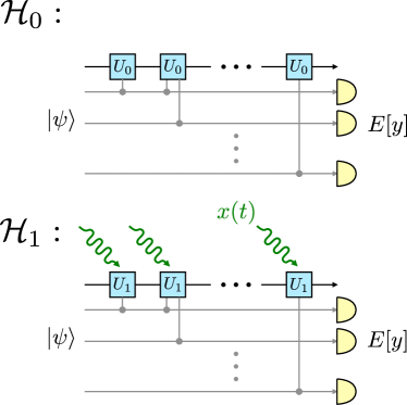
Figure 1: Quantum-circuit diagrams for the waveform detection problem. The quantum system is modeled as a pure state $|\psi\rangle$ with unitary evolution ($U_{0}$ or $U_{1}$) under each hypothesis ($\mathcal{H}_{0}$ or $\mathcal{H}_{1}$) in a large enough Hilbert space for a given classical waveform $x(t)$, which perturbs the evolution under $\mathcal{H}_{1}$. If $x(t)$ is stochastic, the final quantum state under $\mathcal{H}_{1}$ is mixed. Measurements are modeled as a positive-operator-valued measure (POVM) $E[y]$ at the final time through the principle of deferred measurement.

This setup can now be cast as a problem of quantum state discrimination between a pure state

$$\rho_{0}\equiv U_{0}|\psi\rangle\langle\psi|U_{0}^{\dagger}$$ (10)

and a mixed state

$$\rho_{1}\equiv\int DxP[x]U_{1}|\psi\rangle\langle\psi|U_{1}^{\dagger}.$$ (11)

Let $|\Psi_{j}\rangle$ be a purification of $\rho_{j}$ in a larger Hilbert space $\mathbb{H}_{A}\otimes\mathbb{H}_{B}$, such that $\rho_{j}=\operatorname{tr}_{B}|\Psi_{j}\rangle\langle\Psi_{j}|$ and $\operatorname{tr}\{E[y]\rho_{j}\}=\operatorname{tr}[(E[y]\otimes 1_{B})|\Psi_{j}\rangle\langle\Psi_{j}|]$, where $1_{B}$ denotes the identity operator with respect to $\mathbb{H}_{B}$. The average error probability is thus lower-bounded by Helstrom (1976):

$$P_{e} \geq\frac{1}{2}\left(1-\sqrt{1-4P_{0}P_{1}|\langle\Psi_{0}|\Psi_{1}\rangle|^{2}}\right),$$ (12)

which is valid for any purification. Hence

$$P_{e} \geq\frac{1}{2}\left(1-\sqrt{1-4P_{0}P_{1}\max_{|\Psi_{0}\rangle,|\Psi_{1}\rangle}\left|\langle\Psi_{0}|\Psi_{1}\rangle\right|^{2}}\right)$$ (13)

$$=\frac{1}{2}\left(1-\sqrt{1-4P_{0}P_{1}F}\right),$$ (14)

where $F$ is the quantum fidelity by Uhlmann’s theorem Nielsen and Chuang (2000):

$$F(\rho_{0},\rho_{1}) \equiv\left(\operatorname{tr}\sqrt{\sqrt{\rho_{1}}\rho_{0}\sqrt{\rho_{1}}}\right)^{2}.$$ (15)

As $\rho_{0}$ is pure, the fidelity is given by

$$F =\langle\psi|U_{0}^{\dagger}\rho_{1}U_{0}|\psi\rangle=\mathbb{E}(F_{x}),$$ (16)

$$F_{x} \equiv\left|\left\langle U_{0}^{\dagger}(t_{f},t_{i})U_{1}(t_{f},t_{i})\right\rangle\right|^{2},$$ (17)

where we have defined classical and quantum averages by

$$\mathbb{E}(\cdot) \equiv\int DxP[x](\cdot),$$ (18)

$$\langle\cdot\rangle \equiv\langle\psi|\cdot|\psi\rangle.$$ (19)

By similar arguments, a quantum bound on the miss probability $P_{01}$ for a given allowable false-alarm probability $P_{10}$ can be derived from the bound for the pure-state case Helstrom (1976):

$$P_{01} \geq\Big{\{}\begin{array}[]{ll}1-[\sqrt{P_{10}F}+\sqrt{(1-P_{10})(1-F)}]^{2},&P_{10}\leq F;\\ 0,&P_{10}\geq F.\end{array}$$ (22)

Note that the latter bound is equally valid if we interchange $P_{01}$ and $P_{10}$; for example, fixing $P_{01}=0$ means $P_{10}\geq F$. Equations (14) and (22) are valid for any POVM and achievable if $x(t)$ is known a priori, such that both $\rho_{0}$ and $\rho_{1}$ are pure Helstrom (1976).

In terms of related prior work at this point, Ou Ou (1996) and Paris Paris (1997) studied quantum limits to interferometry in the context of detection, while Childs et al. Childs et al. (2000), Acín et al. Acín (2001); Acín et al. (2001), and D’Ariano et al. D’Ariano et al. (2001) also studied unitary or channel discrimination, but all of them did not consider time-dependent Hamiltonians, which are the subject of interest here.

A key step towards simplifying Eq. (17) is to recognize that

$$U_{0}^{\dagger}(t_{f},t_{i})U_{1}(t_{f},t_{i}) =\mathcal{T}\exp\left[-\frac{i}{\hbar}\int_{t_{i}}^{t_{f}}dt\Delta H_{0}(x(t),t)\right],$$ (23)

where

$$\Delta H_{0}(x(t),t)\equiv U_{0}^{\dagger}(t,t_{i})\Delta H(x(t),t)U_{0}(t,t_{i})$$ (24)

is $\Delta H$ in the interaction picture Braginsky and Khalili (1992). In general, Eq. (17) can then be expanded in a Dyson series and evaluated using perturbation theory Peskin and Schroeder (1995). To derive analytic expressions, however, we shall be more specific about the Hamiltonians and the initial quantum state.

III Force detection with a linear Gaussian system

Assume that $x$ is a force on a quantum object with position operator $q$, so that

$$\Delta H=-qx,$$ (25)

and the conditional fidelity $F_{x}$ becomes

$$F_{x} =\left|\left\langle\mathcal{T}\exp\left[\frac{i}{\hbar}\int_{t_{i}}^{t_{f}}dtq_{0}(t)x(t)\right]\right\rangle\right|^{2},$$ (26)

with $q_{0}(t)$ obeying equations of motion under the null hypothesis $\mathcal{H}_{0}$ in the interaction picture. The $\langle\cdot\rangle$ expression in Eq. (26) is a noncommutative version of the characteristic functional Gardiner and Zoller (2004). To simplify it, assume further that $H_{0}$ consists of terms at most quadratic with respect to canonical position or momentum operators, such that the equations of motion are linear and $q_{0}(t)$ depends linearly on the initial-time canonical operators. Let $Z(t)$ be a column vector of canonical position/momentum operators, including $q_{0}(t)$, that obey the equation of motion

$$\frac{dZ(t)}{dt} =G(t)Z(t)+J(t)$$ (27)

under hypothesis $\mathcal{H}_{0}$, where $G(t)$ is a drift matrix and $J(t)$ is a source vector, both consisting of real numbers. $q_{0}(t)$ can then be written as

$$q_{0}(t) =V_{q}(t,t_{i})Z(t_{i})+\int_{t_{i}}^{t}d\tau V_{q}(t,\tau)J(\tau),$$ (28)

where $V_{q}(t,t_{i})$ is a row vector and a function of $G(t)$. This gives

$$\frac{1}{\hbar}\int_{t_{i}}^{t_{f}}dtq_{0}(t)x(t)=\kappa^{\top}Z(t_{i})+\phi,$$ (29)

$$\kappa^{\top}\equiv\frac{1}{\hbar}\int_{t_{i}}^{t_{f}}dtx(t)V_{q}(t,t_{i}),$$ (30)

$$\phi\equiv\frac{1}{\hbar}\int_{t_{i}}^{t_{f}}dtx(t)\int_{t_{i}}^{t}d\tau V_{q}(t,\tau)J(\tau).$$ (31)

With $F_{x}$ now given by

$$F_{x} =\left|\left\langle\mathcal{T}\exp\left[i\kappa^{\top}Z(t_{i})+i\phi\right]\right\rangle\right|^{2},$$ (32)

the time-ordering operator becomes redundant:

$$F_{x} =\left|\langle\psi|\exp\left[i\kappa^{\top}Z(t_{i})\right]|\psi\rangle\right|^{2}.$$ (33)

This expression can be simplified using the Wigner representation $W(z,t_{i})$ of $|\psi\rangle$, which has the following property Walls and Milburn (2008):

$$\langle\psi|\exp\left[i\kappa^{\top}Z(t_{i})\right]|\psi\rangle =\int dzW(z,t_{i})\exp(i\kappa^{\top}z),$$ (34)

where $z$ is a column vector of phase-space variables. Assuming further that $W(z,t_{i})$ is Gaussian with mean vector $\bar{z}$ and covariance matrix $\Sigma$, we obtain an analytic expression for $F_{x}$:

$$F_{x} =\left|\int dzW(z,t_{i})\exp(i\kappa^{\top}z)\right|^{2}$$ (35)

$$=\exp\left(-\kappa^{\top}\Sigma\kappa\right)$$ (36)

$$=\exp\left[-\frac{1}{\hbar^{2}}\int_{t_{i}}^{t_{f}}dt\int_{t_{i}}^{t_{f}}dt^{\prime}x(t)\Sigma_{q}(t,t^{\prime})x(t^{\prime})\right],$$ (37)

$$\Sigma_{q}(t,t^{\prime}) \equiv V_{q}(t,t_{i})\Sigma V_{q}^{\top}(t^{\prime},t_{i}).$$ (38)

The covariance matrix is given by the Weyl-ordered second moment:

$$\Sigma_{jk} =\frac{1}{2}\left\langle Z_{j}(t_{i})Z_{k}(t_{i})+Z_{k}(t_{i})Z_{j}(t_{i})\right\rangle$$

$$\quad-\left\langle Z_{j}(t_{i})\right\rangle\left\langle Z_{k}(t_{i})\right\rangle.$$ (39)

Hence

$$\Sigma_{q}(t,t^{\prime}) =\frac{1}{2}\left\langle q_{0}(t)q_{0}(t^{\prime})+q_{0}(t^{\prime})q_{0}(t)\right\rangle-\left\langle q_{0}(t)\right\rangle\left\langle q_{0}(t^{\prime})\right\rangle.$$ (40)

It is interesting to note that the expression given by $-\ln F_{x}$ in Eq. (37) coincides with the one proposed in Refs. Braginsky and Khalili (1992); Braginsky et al. (1999) as an upper quantum limit on the force-sensing signal-to-noise ratio, and $4\Sigma_{q}(t,t^{\prime})/\hbar^{2}$ is equal to the quantum Fisher information in the quantum Cramér-Rao bound for waveform estimation Tsang et al. (2011). The relation of this expression to the fidelity and the detection error bounds is a novel result here, however.

If the statistics of $q_{0}(t)$ can be approximated as stationary; viz.,

$$\Sigma_{q}(t,t^{\prime})=\int_{-\infty}^{\infty}\frac{d\omega}{2\pi}S_{q}(\omega)\exp[-i\omega(t-t^{\prime})],$$ (41)

$F_{x}$ becomes

$$F_{x} =\exp\left[-\frac{1}{\hbar^{2}}\int_{-\infty}^{\infty}\frac{d\omega}{2\pi}S_{q}(\omega)|x(\omega)|^{2}\right],$$ (42)

$$x(\omega) \equiv\int_{t_{i}}^{t_{f}}dtx(t)\exp(i\omega t).$$ (43)

For example, if

$$x(t)=X\cos(\Omega t+\theta)$$ (44)

is a sinusoid,

$$F_{x} \approx\exp\left[-\frac{T}{\hbar^{2}}S_{q}(\Omega)X^{2}\right], T \equiv t_{f}-t_{i}.$$ (45)

These expressions for the fidelity suggest that, for a given $x(t)$, there is a fundamental trade-off between force detection performance and precision in detector position.

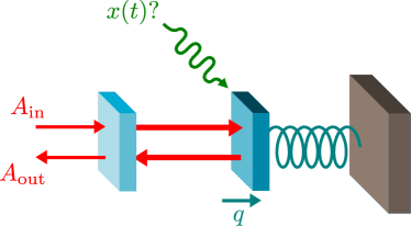
Figure 2: A cavity optomechanical force detector. An optical cavity with a moving mirror is pumped on-resonance with an input field $A_{\textrm{in}}$, and the output field $A_{\rm out}$ is measured to infer whether a force $x(t)$ has perturbed the motion of the mirror.

IV Optomechanics

Suppose now that the mechanical object is a moving mirror of an optical cavity probed by a continuous-wave optical beam, the phase of which is modulated by the object position and the intensity of which exerts a measurement backaction via radiation pressure on the object, as depicted in Fig. 2. This setup provides a basic and often sufficient model for more complex optomechanical force detectors. Let the output field operator under hypothesis $\mathcal{H}_{j}$ be

$$A_{\textrm{out}j}(t) \approx K_{1}(t)*A_{\textrm{in}}(t)+i\mathcal{A}K_{2}(t)*q_{j}(t),$$ (46)

where

$$a(t)*b(t)\equiv\int_{-\infty}^{\infty}d\tau a(t-\tau)b(\tau)$$ (47)

denotes convolution,

$$K_{n}(t)\equiv\int_{-\infty}^{\infty}\frac{d\omega}{2\pi}K_{n}(\omega)\exp(-i\omega t)$$ (48)

is an impulse-response function with

$$K_{1}(\omega) \equiv\frac{i\omega+\gamma}{-i\omega+\gamma},$$ (49)

$$K_{2}(\omega) \equiv\frac{2\omega_{0}}{L}\frac{1}{-i\omega+\gamma}$$ (50)

in the frequency domain, $\mathcal{A}$ is the input mean field, $\omega_{0}$ is the optical carrier frequency, $L$ is the cavity length, and $\gamma$ is the optical cavity decay rate Tsang and Caves (2010). $q_{j}(t)$ is the position operator under each hypothesis, which can be written as Tsang and Caves (2010)

$$q_{0}(t) \approx K_{3}(t)*\hbar K_{2}(t)*\xi(t),$$ (51)

$$q_{1}(t) \approx K_{3}(t)*[\hbar K_{2}(t)*\xi(t)+x(t)],$$ (52)

where $K_{3}(t)$ is another impulse response function that transfers a force to the position,

$$\xi\approx\mathcal{A}^{*}\Delta A_{\textrm{in}}(t)+\mathcal{A}\Delta A_{\textrm{in}}^{\dagger}(t)$$ (53)

is the backaction noise, and the transient solutions are assumed to have decayed to zero. Defining

$$K_{4}(t)\equiv K_{3}(t)*K_{2}(t),$$ (54)

such that the position power spectral density is

$$S_{q}(\omega)=\hbar^{2}|K_{4}(\omega)|^{2}S_{\xi}(\omega),$$ (55)

we obtain

$$F_{x} =\exp\left[-\int_{-\infty}^{\infty}\frac{d\omega}{2\pi}S_{\xi}(\omega)|K_{4}(\omega)x(\omega)|^{2}\right].$$ (56)

The backaction noise $\xi$ that appears in the output field, in addition to the shot noise in $A_{\textrm{in}}$, can limit the detection performance at the so-called standard quantum limit Braginsky and Khalili (1992); Braginsky et al. (1980); Caves et al. (1980); Caves (1985). This does not seem to agree with the fundamental quantum limits in terms of Eq. (56), which suggest that increased fluctuations in $q_{0}(t)$ due to $\xi(t)$ can improve the detection. Fortunately, it is now known that the backaction noise can be removed from the output field Yuen (1983); Ozawa (1988); Tsang and Caves (2010, 2012); Caniard et al. (2007); Julsgaard et al. (2001); Hammerer et al. (2009); Wasilewski et al. (2010); Kimble et al. (2001). One method, called quantum-noise cancellation (QNC), involves passing the optical beam through another quantum system that has the effective dynamics of an optomechanical system with negative mass Tsang and Caves (2010, 2012); Julsgaard et al. (2001); Hammerer et al. (2009); Wasilewski et al. (2010). With the backaction noise removed, the output fields become

$$A_{\textrm{out}0}(t) \approx K_{1}(t)*A_{\textrm{in}}(t),$$ (57)

$$A_{\textrm{out}1}(t) \approx K_{1}(t)*A_{\textrm{in}}(t)+i\mathcal{A}K_{2}(t)*K_{3}(t)*x(t).$$ (58)

If the phase quadrature of $A_{\textrm{out}j}(t)$ is measured by homodyne detection, the outputs can be written as

$$y_{0}(t) \approx\eta(t),$$ (59)

$$y_{1}(t) \approx\eta(t)+K_{2}(t)*K_{3}(t)*x(t),$$ (60)

$$\eta(t) \equiv\frac{1}{2i|\mathcal{A}|^{2}}[\mathcal{A}^{*}K_{1}(t)*\Delta A_{\textrm{in}}(t)-\mathcal{A}K_{1}^{*}(t)*\Delta A_{\textrm{in}}^{\dagger}(t)].$$ (61)

The power spectral densities of $\xi(t)$ and $\eta(t)$ satisfy an uncertainty relation Braginsky and Khalili (1992):

$$S_{\xi}(\omega)S_{\eta}(\omega) \geq\frac{1}{4}.$$ (62)

The detection problem described by Eqs. (59) and (60) becomes a classical one with additive Gaussian noise, a scenario that has been studied extensively in gravitational-wave detection Flanagan and Hughes (1998a, b).

V Error bounds for deterministic waveform detection

Suppose that $x(t)$ is known a priori. It is then well known that the error probabilities for the detection problem described by Eqs. (59) and (60) using a likelihood-ratio test are Van Trees (2001a)

$$P_{10,\textrm{hom}} =\frac{1}{2}\operatorname{erfc}\left(\sigma+\frac{\lambda}{4\sigma}\right),$$ (63)

$$P_{01,\textrm{hom}} =\frac{1}{2}\operatorname{erfc}\left(\sigma-\frac{\lambda}{4\sigma}\right),$$ (64)

where

$$\operatorname{erfc}u \equiv\frac{2}{\sqrt{\pi}}\int_{u}^{\infty}dv\exp(-v^{2}),$$ (65)

$\lambda$ is the threshold in the likelihood-ratio test, which can be adjusted according to the desired criterion, and $\sigma$ is a signal-to-noise ratio given by

$$\sigma^{2}\approx\frac{1}{8}\int_{-\infty}^{\infty}\frac{d\omega}{2\pi}\frac{|K_{4}(\omega)x(\omega)|^{2}}{S_{\eta}(\omega)}$$ (66)

for a long observation time relative to the duration of $x(t)$ plus the decay time of $K_{4}(t)$. To compare homodyne detection with the quantum limits, suppose that the duration of $x(t)$ is long and $\sigma^{2}$ increases at least linearly with $T$, so that we can define an error exponent as the asymptotic decay rate of an error probability in the long-time limit. For simplicity, we consider here only the exponent of the higher error probability:

$$\Gamma \equiv-\lim_{T\to\infty}\frac{1}{T}\ln\max\left\{P_{10},P_{01}\right\}.$$ (67)

Although this asymptotic limit may not be relevant to gravitational-wave detectors in the near future, the error probabilities for which are anticipated to remain high, we focus on this limit to obtain simple analytic results, which allow us to gain useful insight into the fundamental physics. More precise calculations of error probabilities are more tedious but should be straightforward following the theory outlined here.

For homodyne detection, the error exponent is

$$\Gamma_{\textrm{hom}} =\frac{\sigma^{2}}{T}=\frac{1}{8T}\int_{-\infty}^{\infty}\frac{d\omega}{2\pi}\frac{|K_{4}(\omega)x(\omega)|^{2}}{S_{\eta}(\omega)}.$$ (68)

The quantum limit, on the other hand, is

$$\quad-\lim_{T\to\infty}\frac{1}{T}\ln\max\left\{P_{10},P_{01}\right\}$$

$$\leq-\lim_{T\to\infty}\frac{1}{T}\ln\max_{P_{0}}P_{e}\leq-\lim_{T\to\infty}\frac{1}{T}\ln F\equiv\Gamma_{F},$$ (69)

which gives

$$\Gamma_{F} =\frac{1}{T}\int_{-\infty}^{\infty}\frac{d\omega}{2\pi}S_{\xi}(\omega)|K_{4}(\omega)x(\omega)|^{2}.$$ (70)

Using the uncertainty relation between $S_{\xi}$ and $S_{\eta}$ in Eq. (62), it can be seen that

$$\Gamma_{\rm hom}\leq\frac{\Gamma_{F}}{2},$$ (71)

that is, the homodyne error exponent is at most half the optimal value. This fact is well known in the context of coherent-state discrimination Helstrom (1976); Cook et al. (2007); Wittmann et al. (2008); Tsujino et al. (2011). The suboptimality of homodyne detection here should be contrasted with the conclusion of Ref. Tsang et al. (2011), which states that homodyne detection together with QNC are sufficient to achieve the quantum limit for the task of waveform estimation.

To see how one can get closer to the quantum limits, let’s go back to Eqs. (57) and (58). Observe that, if the input field is in a coherent state, the output field is also in a coherent state (in the Schrödinger picture) under each hypothesis. This means that existing results for coherent-state discrimination can be used to construct an optimal receiver. The Kennedy receiver, for example, displaces the output field so that it becomes vacuum under $\mathcal{H}_{0}$ and then detects the presence of any output photon Helstrom (1976). Any detected photon means that $\mathcal{H}_{1}$ must be true. Deciding on $\mathcal{H}_{0}$ if no photon is detected and $\mathcal{H}_{1}$ otherwise, the false-alarm probability $P_{10}$ is zero, while the miss probability is the probability of detecting no photon given $\mathcal{H}_{1}$, or

$$P_{01,\textrm{Ken}} =\exp\left[-\int_{t_{i}}^{t_{f}}dt\left|\mathcal{A}K_{2}(t)*K_{3}(t)*x(t)\right|^{2}\right].$$ (72)

For a long observation time with $S_{\xi}=|\mathcal{A}|^{2}$ for a coherent state,

$$P_{01,\textrm{Ken}} \approx\exp\left[-\int_{-\infty}^{\infty}\frac{d\omega}{2\pi}S_{\xi}|K_{4}(\omega)x(\omega)|^{2}\right]=F,$$ (73)

which makes the Kennedy receiver optimal under the Neyman-Pearson criterion in the case of $P_{10}=0$ according to Eq. (22) and also achieve the optimal error exponent:

$$\Gamma_{\textrm{Ken}} =-\lim_{T\to\infty}\frac{1}{T}\ln P_{01,\textrm{Ken}}=\Gamma_{F}.$$ (74)

The Kennedy receiver can be integrated with the QNC setup; an example is shown in Fig. 3. The Dolinar receiver, which updates the displacement field continuously according to the measurement record, can further improve the average error probability slightly to saturate the lower limit given by Eq. (14) Helstrom (1976); Cook et al. (2007). Other more recently proposed receivers may also be used here to beat the homodyne limit Wittmann et al. (2008); Tsujino et al. (2011).

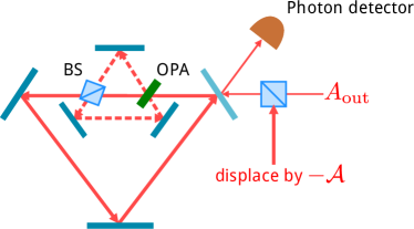
Figure 3: An integrated QNC-Kennedy receiver. The output field $A_{\textrm{out}}$ from the optomechanical force detector in Fig. 2 is displaced by $-\mathcal{A}$ and then passed through an optical setup that removes the measurement backaction noise. The dash arrows represent a red-detuned optical cavity mode that mimics a negative-mass oscillator and interacts with the optical probe field via a beam splitter (BS) and a two-mode optical parametric amplifier (OPA). Details of how this setup works can be found in Refs. Tsang and Caves (2010, 2012). If the field $A_{\rm in}$ is in a coherent state, the final output field should be in a vacuum state under the null hypothesis $\mathcal{H}_{0}$. Any photon detected at the output indicates that $\mathcal{H}_{1}$ must be true.

VI Error bounds for stochastic waveform detection

Consider now a stochastic $x(t)$, which should be relevant to the detection of stochastic backgrounds of gravitational waves Regimbau (2011). Since $F_{x}$ is Gaussian,

$$F =\int DxP[x]\exp\left[-\frac{1}{\hbar^{2}}\int dtdt^{\prime}x(t)\Sigma_{q}(t,t^{\prime})x(t^{\prime})\right]$$ (75)

can be computed analytically if the prior $P[x]$ is also Gaussian. Here we shall use a discrete-time approach and take the continuous limit at the end of our calculations. If $x(t)$ is a zero-mean Gaussian process with covariance

$$\Sigma_{x}(t,t^{\prime})\equiv\mathbb{E}[x(t)x(t^{\prime})],$$ (76)

it can be discretized as

$$x \equiv(x_{0},\dots,x_{N-1})^{\top},$$ (77)

$$DxP[x] \approx dx_{0}\dots dx_{N-1}\frac{1}{\sqrt{(2\pi)^{N}\det\Sigma_{x}}}$$

$$\quad\times\exp\left(-\frac{1}{2}x^{\top}\Sigma_{x}^{-1}x\right),$$ (78)

$$\Sigma_{x} \equiv\mathbb{E}(xx^{\top}).$$ (79)

The fidelity then becomes a finite-dimensional Gaussian integral:

$$F \approx\int dx_{0}\dots dx_{N-1}\frac{1}{\sqrt{(2\pi)^{N}\det\Sigma_{x}}}$$

$$\quad\times\exp\left(-\frac{1}{2}x^{\top}\Sigma_{x}^{-1}x-\frac{\delta t^{2}}{\hbar^{2}}x^{\top}\Sigma_{q}x\right)$$ (80)

$$=\sqrt{\frac{\det(\Sigma_{x}^{-1}+2\delta t^{2}\Sigma_{q}/\hbar^{2})^{-1}}{\det\Sigma_{x}}}$$ (81)

$$=\left[\det\left(I+\frac{2\delta t^{2}}{\hbar^{2}}\Sigma_{q}\Sigma_{x}\right)\right]^{-1/2}$$ (82)

$$=\exp\left[-\frac{1}{2}\operatorname{tr}\ln\left(I+\frac{2\delta t^{2}}{\hbar^{2}}\Sigma_{q}\Sigma_{x}\right)\right]$$ (83)

$$=\exp\left(-\frac{1}{2}\sum_{\omega}\ln\lambda_{\omega}\right),$$ (84)

where $\lambda_{\omega}$ are the eigenvalues of the matrix

$$C\equiv I+\frac{2\delta t^{2}}{\hbar^{2}}\Sigma_{q}\Sigma_{x}.$$ (85)

If $\Sigma_{q}(t,t^{\prime})$ and $\Sigma_{x}(t,t^{\prime})$ are both stationary; viz.,

$$\Sigma_{q}(t,t^{\prime}) =\sigma_{q}(t-t^{\prime}),$$ (86)

$$\Sigma_{x}(t,t^{\prime}) =\sigma_{x}(t-t^{\prime}),$$ (87)

they can be modeled as circulant matrices in discrete time, so that $C$ is also circulant, with eigenvalues given by the discrete Fourier transform of a row or column vector of the matrix. Taking the continuous-time limit using

$$\sum_{\omega}\to T\int_{-\infty}^{\infty}\frac{d\omega}{2\pi},$$ (88)

we get

$$F =\exp(-\Gamma_{F}T),$$ (89)

$$\Gamma_{F} =\frac{1}{2}\int_{-\infty}^{\infty}\frac{d\omega}{2\pi}\ln\left[1+\frac{2}{\hbar^{2}}S_{q}(\omega)S_{x}(\omega)\right],$$ (90)

$$S_{q}(\omega) \equiv\int_{-\infty}^{\infty}dt\sigma_{q}(t)\exp(i\omega t),$$ (91)

$$S_{x}(\omega) \equiv\int_{-\infty}^{\infty}dt\sigma_{x}(t)\exp(i\omega t).$$ (92)

This fidelity expression can then be used in the detection error bounds.

For homodyne detection, the error exponent is more complicated for stochastic waveform detection and given by the Chernoff distance Van Trees (2001b); [][; Chap.~10.]levy:

$$\quad\Gamma_{\rm hom}$$

$$=\sup_{0\leq s\leq 1}\frac{1}{2}\int_{-\infty}^{\infty}\frac{d\omega}{2\pi}\ln\frac{1+(1-s)|K_{4}(\omega)|^{2}S_{x}(\omega)/S_{\eta}(\omega)}{[1+|K_{4}(\omega)|^{2}S_{x}(\omega)/S_{\eta}(\omega)]^{1-s}}.$$ (93)

The performance of homodyne detection relative to the quantum limits then depends on the specific form of $|K_{4}(\omega)|^{2}S_{x}(\omega)$. The Kennedy receiver, on the other hand, is still applicable here, as the output is still a coherent state under $\mathcal{H}_{0}$. The false-alarm probability is still zero, and the miss probability is now

$$P_{01,\textrm{Ken}} \approx\mathbb{E}\exp\left[-\int_{-\infty}^{\infty}\frac{d\omega}{2\pi}S_{\xi}(\omega)|K_{4}(\omega)x(\omega)|^{2}\right]\approx F,$$ (94)

which means that the Kennedy receiver remains optimal, both in terms of the Neyman-Pearson criterion in the case of $P_{10}=0$ and the error exponent. Whether other receivers can do even better and saturate the other quantum bounds is a more difficult question, as the output field under $\mathcal{H}_{1}$ is now in a mixed state and the fidelity lower bounds may not be achievable.

The use of Kennedy or Dolinar receivers assumes coherent states at the output, which is the case only if the backaction noise cancellation is complete and quantum shot noise in the input beam is the only source of noise at the output. Although such assumptions are highly idealistic, especially for current gravitational-wave detectors, the ideal scenario shows that the quantum bounds proposed here are in principle achievable using known optics technology. Optimal discrimination of squeezed or other Gaussian states remains a topic of current research Tan et al. (2008); Guha and Erkmen (2009); Pirandola (2011) and may be useful for future gravitational-wave detectors that use squeezed light The LIGO Scientific Collaboration (2011). Generalization of the results here to multi-waveform discrimination should also be useful for gravitational-wave astronomy Flanagan and Hughes (1998a, b) and may be done by following Refs. Helstrom (1976); Yuen et al. (1975); Bondurant (1993).

VII Outlook

Now that quantum limits to waveform detection have been discovered, the natural next question to ask is how they can be approached in practice. In the case of optomechanical force detection, the requirements are quantum shot noise as the only source of noise at the output and an appropriate receiver, such as the Kennedy receiver. A proof-of-concept experimental demonstration of waveform detection approaching the shot-noise limits based on Eq. (56) should be well within reach of current quantum optics technology. To demonstrate the trade-off between force detection performance and detector localization suggested by Eq. (42) with optomechanics, however, can be much more challenging, as it would require quantum backaction noise to dominate the detector position fluctuation but become negligible in the output via QNC. A more promising candidate for this demonstration is atomic spin ensembles, with which backaction-noise-canceled magnetometry has already been realized Wasilewski et al. (2010). The likelihood-ratio formulas derived in Ref. Tsang (2012a) should be used in practice instead of the ideal-case decision rules discussed here to account for any excess noise.

In terms of potential further theoretical work, it should be useful to generalize beyond the assumptions of scalar waveform, linear Gaussian systems, optical coherent states, stationary processes, and long observation time used here. The fidelity expressions derived here may also be useful for the study of waveform estimation Tsang et al. (2011), either as an alternative way of deriving the quantum Fisher information via a Taylor-series expansion Braunstein and Caves (1994) or used directly in the quantum Ziv-Zakai bound Tsang (2012b).

From a more conceptual point of view, this study, together with the earlier work on waveform estimation Tsang et al. (2011), shows that the concepts of states, effects, and operations fade into background when dealing with dynamical quantum information systems, and multi-time quantum statistics, through the use of Heisenberg or interaction picture, take the center stage. It may be interesting to explore whether this perspective has any relevance to other dynamical quantum information systems, such as quantum computers Nielsen and Chuang (2000), and the study of quantum correlations Horodecki et al. (2009).

References

- Schnabel et al. (2010) R. Schnabel, N. Mavalvala, D. E. McClelland, and P. K. Lam, Nature Commun. 1, 121 (2010).
- Chu (2002) S. Chu, Nature (London) 416, 206 (2002).
- Budker and Romalis (2007) D. Budker and M. Romalis, Nature Phys. 3, 227 (2007).
- Giovannetti et al. (2004) V. Giovannetti, L. Maccone, and S. Lloyd, Science 306, 1330 (2004).
- Braginsky and Khalili (1992) V. B. Braginsky and F. Y. Khalili, Quantum Measurement (Cambridge University Press, Cambridge, 1992).
- Braginsky et al. (1980) V. B. Braginsky, Y. I. Vorontsov, and K. S. Thorne, Science 209, 547 (1980).
- Caves et al. (1980) C. M. Caves, K. S. Thorne, R. W. P. Drever, V. D. Sandberg, and M. Zimmermann, Rev. Mod. Phys. 52, 341 (1980).
- Helstrom (1976) C. W. Helstrom, Quantum Detection and Estimation Theory (Academic Press, New York, 1976).
- Holevo (2001) A. S. Holevo, Statistical Structure of Quantum Theory (Springer-Verlag, Berlin, 2001).
- Kraus (1983) K. Kraus, States, Effects, and Operations: Fundamental Notions of Quantum Theory (Springer, Berlin, 1983).
- Aspelmeyer et al. (2010) M. Aspelmeyer, S. Gröblacher, K. Hammerer, and N. Kiesel, J. Opt. Soc. Am. B 27, A189 (2010).
- Van Trees (2001a) H. L. Van Trees, Detection, Estimation, and Modulation Theory, Part I (Wiley, New York, 2001).
- Yuen (1983) H. P. Yuen, Phys. Rev. Lett. 51, 719 (1983).
- Ozawa (1988) M. Ozawa, Phys. Rev. Lett. 60, 385 (1988).
- Caves (1985) C. M. Caves, Phys. Rev. Lett. 54, 2465 (1985).
- Tsang et al. (2011) M. Tsang, H. M. Wiseman, and C. M. Caves, Phys. Rev. Lett. 106, 090401 (2011).
- Tsang and Caves (2010) M. Tsang and C. M. Caves, Phys. Rev. Lett. 105, 123601 (2010).
- Tsang and Caves (2012) M. Tsang and C. M. Caves, Phys. Rev. X 2, 031016 (2012).
- Caniard et al. (2007) T. Caniard, P. Verlot, T. Briant, P.-F. Cohadon, and A. Heidmann, Phys. Rev. Lett. 99, 110801 (2007).
- Julsgaard et al. (2001) B. Julsgaard, A. Kozhekin, and E. S. Polzik, Nature (London) 413, 400 (2001).
- Hammerer et al. (2009) K. Hammerer, M. Aspelmeyer, E. S. Polzik, and P. Zoller, Phys. Rev. Lett. 102, 020501 (2009).
- Wasilewski et al. (2010) W. Wasilewski, K. Jensen, H. Krauter, J. J. Renema, M. V. Balabas, and E. S. Polzik, Phys. Rev. Lett. 104, 133601 (2010).
- Cook et al. (2007) R. L. Cook, P. J. Martin, and J. M. Geremia, Nature (London) 446, 774 (2007).
- Nielsen and Chuang (2000) M. A. Nielsen and I. L. Chuang, Quantum Computation and Quantum Information (Cambridge University Press, Cambridge, 2000).
- Caves and Shaji (2010) C. M. Caves and A. Shaji, Opt. Commun. 283, 695 (2010).
- Ou (1996) Z. Y. Ou, Phys. Rev. Lett. 77, 2352 (1996).
- Paris (1997) M. G. A. Paris, Phys. Lett. A 225, 23 (1997).
- Childs et al. (2000) A. M. Childs, J. Preskill, and J. Renes, J. Mod. Opt. 47, 155 (2000).
- Acín (2001) A. Acín, Phys. Rev. Lett. 87, 177901 (2001).
- Acín et al. (2001) A. Acín, E. Jané, and G. Vidal, Phys. Rev. A 64, 050302(R) (2001).
- D’Ariano et al. (2001) G. M. D’Ariano, P. Lo Presti, and M. G. A. Paris, Phys. Rev. Lett. 87, 270404 (2001).
- Peskin and Schroeder (1995) M. E. Peskin and D. V. Schroeder, An Introduction to Quantum Field Theory (Addison-Wesley, Reading, 1995).
- Gardiner and Zoller (2004) C. W. Gardiner and P. Zoller, Quantum Noise (Springer-Verlag, Berlin, 2004).
- Walls and Milburn (2008) D. F. Walls and G. J. Milburn, Quantum Optics (Springer-Verlag, Berlin, 2008).
- Braginsky et al. (1999) V. B. Braginsky, M. L. Gorodetsky, Y. F. Khalili, and K. S. Thorne, “Energetic quantum limit in large-scale interferometers,” (1999), arXiv:gr-qc/9907057 .
- Kimble et al. (2001) H. J. Kimble, Y. Levin, A. B. Matsko, K. S. Thorne, and S. P. Vyatchanin, Phys. Rev. D 65, 022002 (2001).
- Flanagan and Hughes (1998a) É. É. Flanagan and S. A. Hughes, Phys. Rev. D 57, 4535 (1998a).
- Flanagan and Hughes (1998b) É. É. Flanagan and S. A. Hughes, Phys. Rev. D 57, 4566 (1998b).
- Wittmann et al. (2008) C. Wittmann, M. Takeoka, K. N. Cassemiro, M. Sasaki, G. Leuchs, and U. L. Andersen, Phys. Rev. Lett. 101, 210501 (2008).
- Tsujino et al. (2011) K. Tsujino, D. Fukuda, G. Fujii, S. Inoue, M. Fujiwara, M. Takeoka, and M. Sasaki, Phys. Rev. Lett. 106, 250503 (2011).
- Regimbau (2011) T. Regimbau, Res. Astron. Astrophys. 11, 369 (2011).
- Van Trees (2001b) H. L. Van Trees, Detection, Estimation, and Modulation Theory. Part III (Wiley, New York, 2001).
- Levy (2008) B. C. Levy, Principles of Signal Detection and Parameter Estimation (Springer, New York, 2008).
- Tan et al. (2008) S. H. Tan, B. I. Erkmen, V. Giovannetti, S. Guha, S. Lloyd, L. Maccone, S. Pirandola, and J. H. Shapiro, Phys. Rev. Lett. 101, 253601 (2008).
- Guha and Erkmen (2009) S. Guha and B. I. Erkmen, Phys. Rev. A 80, 052310 (2009).
- Pirandola (2011) S. Pirandola, Phys. Rev. Lett. 106, 090504 (2011).
- The LIGO Scientific Collaboration (2011) The LIGO Scientific Collaboration, Nature Phys. 7, 962 (2011).
- Yuen et al. (1975) H. P. Yuen, R. S. Kennedy, and M. Lax, IEEE Trans. Inf. Theor. 21, 125 (1975).
- Bondurant (1993) R. S. Bondurant, Opt. Lett. 18, 1896 (1993).
- Tsang (2012a) M. Tsang, Phys. Rev. Lett. 108, 170502 (2012a).
- Braunstein and Caves (1994) S. L. Braunstein and C. M. Caves, Phys. Rev. Lett. 72, 3439 (1994).
- Tsang (2012b) M. Tsang, Phys. Rev. Lett. 108, 230401 (2012b).
- Horodecki et al. (2009) R. Horodecki, P. Horodecki, M. Horodecki, and K. Horodecki, Rev. Mod. Phys. 81, 865 (2009).