Matrix product states for critical spin chains:
finite size scaling versus finite entanglement scaling

Abstract

We investigate the use of matrix product states (MPS) to approximate ground states of critical quantum spin chains with periodic boundary conditions (PBC). We identify two regimes in the $(N,D)$ parameter plane, where $N$ is the size of the spin chain and $D$ is the dimension of the MPS matrices. In the first regime MPS can be used to perform finite size scaling (FSS). In the complementary regime the MPS simulations show instead the clear signature of finite entanglement scaling (FES). In the thermodynamic limit (or large $N$ limit), only MPS in the FSS regime maintain a finite overlap with the exact ground state. This observation has implications on how to correctly perform FSS with MPS, as well as on the performance of recent MPS algorithms for systems with PBC. It also gives clear evidence that critical models can actually be simulated very well with MPS by using the right scaling relations; in the appendix, we give an alternative derivation of the result of Pollmann et al. [Phys. Rev. Lett. 102, 255701 (2009)] relating the bond dimension of the MPS to an effective correlation length.

I Introduction

Quantum many body systems are very hard to study due to the exponential growth of their Hilbert space with the number of constituents. One possible cure to this issue for one dimensional systems is to describe their ground states as matrix product states (MPS) Klümper et al. (1993); Verstraete et al. (2008); Schollwöck (2011). This family of states is known to be well suited to study gaped 1D phases Fannes et al. (1992) where for generic systems almost exact results can be obtained with matrices whose size does not depend on the size of the system. Even more, for several gapped 1D systems the exact ground state can be expressed in terms of translationally invariant MPS with very small bond dimension Affleck et al. (1987); Fannes et al. (1992). Gapless 1D phases are harder to simulate with MPS since the size of the matrices necessary to obtain good approximations of their ground states increases polynomially with the size of the system. This is particularly unfortunate since the universal low energy information encoded in the gapless phase becomes apparent only for large systems.

Luckily such universal information is also encoded in the way a state approaches the thermodynamic limit and one can extract it by using the celebrated finite size scaling (FSS) technique Barber (1983). This technique amounts to study larger and larger systems in a gapless phase (that due to the finite size of the system becomes gapped) and extract universal properties through the dependence of the observables on the system size.

In the context of MPS, one can use an alternative approach to study gapless phases. It is called finite entanglement scaling (FES) Tagliacozzo et al. (2008) and amounts to study the scaling of the expectation value of observables in the ground state of infinite chains described by MPS with fixed bond dimension and thus finite entanglement .

Both the existence of FSS and FES close to a conformal fixed point are a direct consequence of conformal invariance Blöte et al. (1986); Pollmann et al. (2009). If $N$ is the chain length and $D$ the MPS bond dimension, then FSS corresponds to taking $D\to\infty$ first and then taking $N\to\infty$, whereas FES consists in taking $N\to\infty$ first and then $D\to\infty$.

An important question to ask is whether FSS and FES provide the same universal information. Since the proposal of FES for simulations with MPS Tagliacozzo et al. (2008) it has been shown that indeed quantities such as critical exponents related to local observables or the central charge of the model can be extracted with the help of this technique Zheng et al. (2011); Rodríguez et al. (2011); Dai et al. (2010); Orus and Wei (2010); McCulloch (2008); Heidrich-Meisner et al. (2009); Zhao et al. (2010), in a similar way as it is normally done with FSS techniques. Here we will show, however, that some care is required in order to differentiate between the effects of FES and those of FSS.

Specifically, we consider critical systems with periodic boundary conditions (PBC), and describe their translationally invariant ground states using translationally invariant MPS. In order to perform FSS one should obtain for each system size $N$ a sequence of increasingly accurate MPS approximations with growing bond dimension $D$, which for large enough $D$ converges to the exact ground state. Importantly, we find that for an intermediate range of values of $D$, for which local observables are already reproduced with high accuracy and show scaling behavior, the MPS approximation is almost completely orthogonal to the exact ground state (resulting e.g. in failure to reproduce correlation functions at distance $N/2$, as previously illustrated in the inset of Fig. 11 and 12 of Ref. Pirvu et al. (2011)). In other words, reasonably converged values of (and/or scaling behavior for) local observables including the ground state energy, are not sufficient criteria to establish that some MPS is a good approximation to the ground state of a critical PBC system. Instead, in order to properly apply FSS, for each system size $N$ one should consider MPS with a bond dimension $D$ larger than some threshold value $D_{0}$, where $D_{0}$ depends both on $N$ and on the spin model.

Our results have important consequences for the design of algorithms that simulate PBC chains with MPS. Simulating PBC systems with MPS is computationally much more expensive Verstraete et al. (2004) than simulating the same system with open boundary conditions (OBC). Nonetheless, when studying critical ground states, systems with PBC are known to approach the thermodynamic limit much faster than systems with OBC, and therefore they offer a much better framework for FSS. For this reason, substantial effort Pippan et al. (2010); Shi and Zhou (2009); Pirvu et al. (2011); Rossini et al. (2011) has been made to try to lower the computational cost of MPS simulations with PBC. Two types of approaches have been pursued. One consists in building a MPS for a finite system with PBC by using the translationally invariant MPS tensor that has been optimized in an infinite chain with OBC Shi and Zhou (2009). This approach is equivalent to a crude approximation of the MPS transfer matrix: the $D^{2}\times D^{2}$ matrix is approximated only by its dominant eigenvector . The second approach Pippan et al. (2010); Pirvu et al. (2011); Rossini et al. (2011) accounts for PBC by retaining more than one eigenvector in the approximation of the transfer matrix. We show in this work that the first approach fails to provide an accurate ground state approximation for critical PBC systems. A detailed comparison of these algorithms can be found in Appendix C.

We will build our arguments by studying two paradigmatic critical spin chains: the quantum Ising model (IS) and the quantum Heisenberg (HB) model, for chains with PBC and linear size $N$. The ground states are encoded in MPS of a given bond dimension $D$. Even if the Hamiltonian is critical, both the finite size of the chain and the finite bond dimension of the MPS induce a gap

$$\Delta E_{N}=\xi_{N}^{-1}=\frac{2\pi\,x_{1}}{N}$$ (1)

$$\Delta E_{D}=\xi_{D}^{-1}\propto D^{-\kappa}$$ (2)

where $x_{1}$ is the smallest critical exponent of the theory Cardy (1986) and $\kappa$ is the exponent for the scaling of the effective correlation length of MPS simulations with finite bond dimension Pollmann et al. (2009); Tagliacozzo et al. (2008). Depending on which of the two gaps dominates, the system is in one of the two regimes

$$\xi_{D}\gg\xi_{N}:\textrm{FSS regime}$$ (3)

$$\xi_{N}\gg\xi_{D}:\textrm{FES regime}$$ (4)

The presence of two regimes in the PBC chain can be intuitively understood in the following way: in the FES regime defined by equation (4) the small dimension of the MPS matrices implies that the system is not aware of its geometry. Thus the boundaries do not play any role. In the FSS regime, defined by equation (3) on the other hand, the size of the matrices is big enough to notice the presence of the boundaries and thus different choices of boundary conditions lead to different MPS.

For simulations where

$$\xi_{N}\simeq\xi_{D}$$ (5)

we find for all values of $N$ and $D$ that are accessible numerically the presence of an abrupt transition between the FSS and FES regimes (for a related work see also Ref. Liu et al. (2010)). One way to observe this transition is by looking at the difference between the exact ground state energy in the thermodynamic limit and the energy of MPS approximations with different $N$ and $D$. For fixed $D$ these plots show a steep transition between the FSS regime where the difference scales like $\propto N^{-2}$ to the FES regime where the difference does not depend on $N$. Another way is to look at the overlap between MPS with different $D$ for fixed chain length $N$: starting off with a MPS with some big $D_{max}$, we look at its overlap with MPS with decreasing $D$. We then observe how the initially smoothly decreasing overlap abruptly drops towards lower values at some $D_{r}$, unambiguously showing the transition to the FES regime. Now the overlap is a global variable and as such indeed aware of the boundary conditions. The main finding of this paper is that states in the FES regime, while possessing the same local universal properties Tagliacozzo et al. (2008) like those in the FSS regime, turn out to have vanishing overlap with them.

We also present a possible technique to determine if a given bond dimension is sufficient to enter the FSS regime, so that we can give the computationally most favorable recipe to access global universal properties that depend on the boundaries (for a discussion of these properties see e.g. Evenbly et al. (2010)).

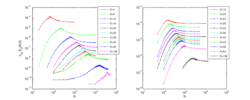
Figure 1: (Color online). Quantum Ising (left) and Heisenberg model (right): Relative precision of the optimal MPS ground state energy for different $D$ as a function of $N$. The position of the hump that can be observed between the small and big $N$ limits of each curve turns out to be proportional to the effective correlation length $\xi_{D}$ of MPS with finite bond dimension.

The paper is organized as follows. We start by introducing the IS and HB models as well as the technique used to simulate them in section II. In section II.1 we present numerical evidence for the presence of the FSS and FES regimes in MPS simulations of PBC chains by looking at the ground state energy. In section II.2 we discuss how to identify the sharp transition between the two regimes by looking at the overlap. Then, in section II.2.1, we give a more detailed view on the transition between the two scaling regimes. Section II.3 gives a recipe for obtaining the minimal bond dimension needed to observe global universal properties of critical systems. In section II.4 we perform a numerical study of the transition and for the IS model we can provide evidence for its persistence in the thermodynamic limit. For the HB model we are not able to do the same due to the coarser precision of our simulations for this model. In section II.5 we provide a numerical analysis of the scaling function for the energy difference that reveals a two-parameter scaling analogous to the one found in the context of critical 2D classical systems by Nishino in Ref. Nishino et al. (1996). We conclude with a discussion of the implications of our results and with a brief outline of future developments.

All technical details are contained in the appendices. There we first provide an alternative way to derive the analytical result for the scaling exponent $\kappa$ in $\xi_{D}\propto D^{\kappa}$, which we find more intuitive than the one given in Pollmann et al. (2009). Then we show how our algorithm can be used in order to extract $\kappa$ from the numerical results for the ground state energy. For the IS model, we are able to provide a numerical confirmation for the persistence of the transition between the FSS and the FES regime in the thermodynamical limit.

II Numerical results

We will use throughout this work the algorithm presented in Pirvu et al. (2011). That algorithm exploits the translational invariance of the models we study by using an ansatz based on translationally invariant MPS. This means that the MPS tensors at each site of the chain are identical thus reducing the cost of the simulation by a factor $N$. The energy is minimized by means of a conjugate gradient method in the subspace spanned by real and symmetric MPS with bond dimension $D$. The computational cost scales like $O(mnD^{3})+O(n^{2}D^{3})$. $m$ and $n$ are parameters whose magnitude depends on the entanglement of the ground state of the model under consideration. For more details on the method we refer the reader to that work. The two paradigmatic models we have considered are the critical quantum Ising model described by the Hamiltonian

$$H_{IS}=-\sum_{i=1}^{N}\sigma_{i}^{z}\sigma_{i+1}^{z}-\sum_{i=1}^{N}\sigma_{i}^{x}\,\,\,,$$ (6)

and the Heisenberg model described by the Hamiltonian

$$H_{HB}=\sum_{i=1}^{N}\vec{S}_{i}\vec{S}_{i+1}=\frac{1}{4}\sum_{i=1}^{N}(\sigma^{x}_{i}\sigma^{x}_{i+1}+\sigma^{y}_{i}\sigma^{y}_{i+1}+\sigma^{z}_{i}\sigma^{z}_{i+1})$$ (7)

where the 1D lattice is considered to be periodic. Both Hamiltonians are critical which means that their gap between the ground state and the first excited state closes as an inverse power of $N$ as described in Eq. 1.

As a matter of fact the analysis in this work was triggered by a comprehensive study of the precision of the algorithm presented in Pirvu et al. (2011). We originally wanted to assess the usability of that method and to this end we simulated a plethora of different configurations $\{N,D\}$ for the IS and the HB models. A selection of these simulation results is shown in Figure 1 where we plot the relative energy precision of simulations with different $D$ for many different chain lengths $N$.

The shape of curves with constant $D$ is very surprising since it shows a fundamental deviation from what we would have expected. Our expectation was that for short chains the precision will be generally better than for long chains and that as $N$ gets bigger and bigger, the precision will eventually saturate from below to the value obtained with the corresponding $D$ when simulating the chain in the thermodynamic limit. Obviously the small $N$ and the big $N$ regimes are in accordance with our expectation. However at some point between these limits we see the emergence of a hump which indicates that something interesting is happening in that region. As a matter of fact we can show that if we interpret the position of the hump as an indicator for the effective correlation length $\xi_{D}$ of MPS with finite $D$, we can reproduce the theoretically predicted result for the scaling of $\xi_{D}$ Pollmann et al. (2009) with very good accuracy (see Appendix A). The results presented in this work provide the general framework to understand the emergence of the hump and to explain what is happening when moving from the left to the right side of Fig.  1.

II.1 Two different regimes for MPS simulations

As already mentioned in the introduction a MPS simulation close to the critical point is an example of a two scale problem. This is not something unexpected as it has been already pointed out in the context of 2D classical systems studied with the corner transfer matrix by Nishino and coworkers Nishino et al. (1996) and in the context of quantum phase transitions in 1D quantum chains with open boundaries by one of the authors (section IIIG of Ref. Tagliacozzo et al. (2008)). In the scenario we are considering, the two scales appearing are i) the correlation length induced by the finite size of the system $N$ of Eq. 1 and ii) the correlation length induced by the size of the matrices $D$ of Eq. 2. Depending on the relation among the two stated in Eqs. 3 and 4, the system will be in one of the two different regimes, respectively the FSS regime or the FES regime.

The approach to the thermodynamic limit of the ground state energy, as function of the relevant parameter $N$ or $D$, is very different in the two regimes so that we can use it as a footprint for them. In the FSS regime indeed it obeys the celebrated result by Cardy and Affleck Blöte et al. (1986); Affleck (1986) from conformal field theory (CFT),

$$E_{0}(N)-E_{0}(\infty)=-\frac{v_{f}\pi c}{6N^{2}}\,\,\,,$$ (8)

where $E_{0}(\infty)$ is the thermodynamic limit, $v_{f}$ is the Fermi velocity and $c$ is the central charge of the considered model. In the thermodynamic limit, several authors have reported that Tagliacozzo et al. (2008); Pirvu et al. (2010); Pollmann et al. (2009)

$$E_{0}(D)-E_{0}(\infty)\propto\frac{\Delta}{D^{\omega}}\,\,\,.$$ (9)

where $\omega=2\kappa$ and $\kappa$ is the same exponent of Eq. 2 and $\Delta$ is a positive non-universal constant. We show below that the same scaling holds also for MPS simulations of finite chains if $N$ is big enough. This happens exactly in the FES regime defined by (4).

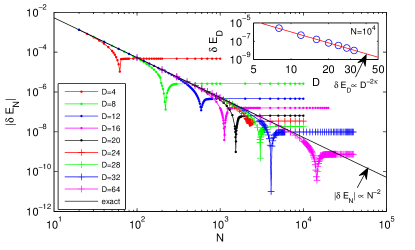
a) b)

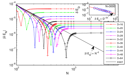
Figure 2: (Color online). a) Quantum Ising model, two regimes for simulations of PBC chains with lengths in the range $20\leq N\leq 4\cdot 10^{4}$, and $D$ in the range $4\leq D\leq 64$. Each line represents simulations performed at fixed $D$ and different $N$. The plots show the absolute value of the difference $\delta E_{N}=E_{0}(N,D=const.)-E_{0}^{\infty}$. The FSS is represented by a diagonal black line following the scaling from Eq. 8. All data sets initially follow this line. The FES regime corresponds to the various horizontal lines, where $\delta E_{N}$ saturates for different $D$ to different values $\delta E_{D}$ that do not depend on $N$. In the inset we collect these values to show that they reproduce the expected behavior of the FES. The two regimes are separated by the appearance of a pronounced peak. Since we plot an absolute value, the peak is nothing more than the change of sign in the difference $E_{0}(N,D)-E_{0}^{\infty}$ when moving from the FSS regime (8) to the FES regime (9). b) The same plot for the HB model tells us that here the FSS is much more difficult to study, since all data-sets deviate very soon from the pure FSS prediction.

The two regimes are very clearly distinguished in Fig. 2 where we present plots of the absolute value of the difference of the ground state energy obtained with MPS simulations and the exact value in the thermodynamic limit

$$\delta E_{N,D}=E_{0}(N,D)-E_{0}(\infty)$$ (10)

as a function of $N$ in a log-log scale. Note that in Fig. 2 we make an abuse of notation by using $\delta E_{N}=(\delta E_{N,D})_{D=const.}$ and $\delta E_{D}=(\delta E_{N,D})_{N=const.}$, which can be only done as long as we specify what the constant value of $D$ or $N$ is. The data is collected from several simulations of the critical IS with PBC for chain lengths in the range $20\leq N\leq 4\cdot 10^{4}$ (panel a) and of the HB with PBC in the range $10^{2}\leq N\leq 5\cdot 10^{3}$ (panel b). $D$ is going in both cases up to $D=64$. Each line in the main plot represents simulations performed for different $N$ at fixed $D$. The FSS predictions of Eq. 8 are straight lines plotted in black. For small $N$, each set of data follows the prediction of Eq. 8, which is a clear signal of the FSS regime. The maximal $N$ for which the FSS prediction holds increases with growing $D$ as expected. However, each set deviates at some big enough $N$ from the FSS prediction to eventually stabilize to a value of the energy difference that only depends on $D$. This is a clear footprint of the FES regime scaling, as described in Eq. 9. In order to confirm this we have added to both panels insets where we have plotted several values of $\delta E_{D}$ for large fixed $N$ as a function of $D$ in a log-log scale. Similar plots in the thermodynamic limit can be found in Pirvu et al. (2010). The linear fits (red lines) in the insets yield $\kappa_{IS}\approx 1.9776$ for $N=10^{4}$ respectively $\kappa_{HB}\approx 1.3025$ for $N=3000$. These values are compatible with the analytical values obtained for $N\to\infty$ in Pollmann et al. (2009), namely $\kappa_{IS}^{anal}\approx 2.03425$ and $\kappa_{HB}^{anal}\approx 1.34405$ and thereby confirm the scaling of Eq. 9.

Note that we are able to obtain much better precision for the IS than for the HB model at at the same computational cost . This is visible by comparing the panel a) to the panel b) and observing that for fixed $D$, the curves for the HB model deviate from the FSS at much lower values of $N$ than the corresponding ones for the IS model.

II.2 The transition between the two regimes

In Figure 2 we can observe that for each line with constant $D$, the FSS region is separated from the FES region by a well distinguishable peak in the absolute value of $\delta E_{N}$. We would now like to show that this transition does not depend on the choice of the observable but that it indicates a global change in the wave function.

To this end we can investigate the trace distance between the exact ground state of a chain with $N$ sites and the MPS obtained from a series of simulations with different $D$. We have chosen the step size in $D$ as small as possible, i.e. $\Delta D=1$. Since the exact ground state wave function is only available for very small systems due to the exponential scaling of the number of parameters, we use as a reference state a MPS approximation of the ground state with very big $D$. For the $N$ range in question, the biggest available bond dimension is $D=64$. Note that the energy difference between the exact ground states and the reference states is much smaller than the difference to the MPS we want to compare to (see Fig. 1).

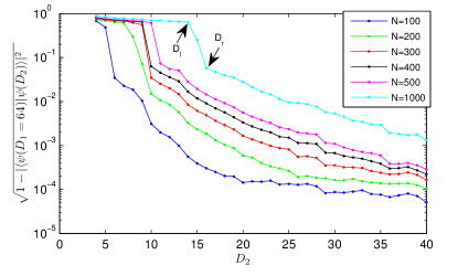
a) b)

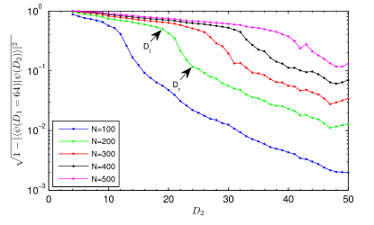
Figure 3: (Color online). a) Quantum Ising model: trace distance between reference states with $D_{1}=64$ and ground state MPS with bond dimensions $D_{2}$ for several different chain lengths. b) Heisenberg model: trace distance between reference states with $D_{1}=64$ and ground state MPS with bond dimensions $D_{2}$ for several different chain lengths.

Figure 3 shows the trace distance between states with relatively small $D$ and reference states for several different chain lengths $N$ for both the IS and the HB models. Note that for every $N$ there is a jump in the trace distance between states that are very far away from the reference state and states that are at least one order of magnitude closer to it. For the IS model the jump is very steep and for each line of constant $N$ we can clearly identify $D_{l}$ as the biggest $D$ in the left (FES) regime and $D_{r}$ as the smallest $D$ in the right (FSS) regime. In this case the appearance of the jump evidently indicates the transition from the FSS regime, where the trace distance is close to zero to the FES regime where the trace distance abruptly increases. For the HB model the transition is much smoother and we can not unambiguously define $D_{l}$ and $D_{r}$ for all lines with constant $N$. This happens presumably due to the fact that taking MPS with $D=64$ as reference states is not accurate enough in the case of the $HB$ model.

However, at least for the IS model, we are now in the position to check if our intuitive expectation, that the transition occurs precisely when the correlation length of the finite size MPS reaches the size of chain as described in Eq. 5, is quantitatively correct. The correlation length of MPS with finite $D$ reads according to Eq. 2 as $\xi(D)=k_{c}\cdot D^{\kappa}$ where $k_{c}$ is a proportionality constant. For our numerical study we obtain the parameters $k_{c}$ and $\kappa$ in the appendix A. We can confirm that for each line of constant $N$ the jump in the trace distance is consistent with our assumption, i.e. $\xi(D_{l})<N<\xi(D_{r})$.

Furthermore we would like to mention that jumps also occur in other quantities at the same $D_{l}$, for instance in the half-chain correlation function reported in Pirvu et al. (2011) (see figure $9$ in that work for a plot of the jump for $N=500$). The fact that the induced correlation length $\xi(D)$ in the FES is smaller than the size of the system, suggests that the state is completely unaware of the presence of the boundaries. This confirms our intuition that MPS in the FSS regime are faithful approximations of finite chains with PBC while MPS in the FES regime do not capture properties related to the boundary conditions.

Summarizing, the main point of this section is that if one is interested in the effects of PBC, results collected for $D$ smaller than $D_{r}$ should not be taken into account. Note that due to the residual dependence on $D$ (see the appendix II.2.1 for details on this point) one still has to extrapolate the results in the limit $D\to\infty$ in order to obtain accurate results. If, on the other hand, one is interested only in local universal quantities (i.e. where boundary conditions are irrelevant), there is no point in simulating the system with PBC and one should rather perform a standard FES study Tagliacozzo et al. (2008).

II.2.1 The real scenario, a complex cross-over induced by corrections to the scaling

We have seen above how in the extremal regions of Figure 2, the simulation results follow the behavior predicted by FSS respectively FES. In the intermediate region however, the simulations display a behavior that can not be attributed to either regime. We would now like to point out that the real picture is somewhat more complex than the two-regime interpretation given above.

The leading scaling behavior given in Equations 8 and 9 represents only the first terms of the series expansion of more complex analytic corrections. Thus these terms are accompanied by higher order terms called corrections to scaling. In order to understand the scenario we must consider the general Taylor expansion of a two variable function. Let us consider two variables $\Delta_{D}$ and $\Delta_{N}$ with the property that $\lim_{D\to\infty}\Delta_{D}=0$ and $\lim_{N\to\infty}\Delta_{N}=0$. Obviously these variables can be identified with the gaps proportional to the inverse of the correlation length induced by the system size $N$ and by the finite matrix dimension $D$ as defined in Eq. 1 and Eq. eq:feg. Part of the scaling ansatz consists in assuming that all universal quantities are universal functions of these two variables.

Let us review the case of a one-scale problem. In this case, by neglecting higher than quadratic terms in the vanishing variable (e.g. $\Delta_{n}$) we get the following series expansion for some universal function $g$

$$g_{\Delta_{N}}=g_{0}+\partial_{\Delta_{N}}g_{0}\Delta_{N}+\frac{1}{2}\partial^{2}_{\Delta_{N}}g_{0}\Delta_{N}^{2}+\cdots$$ (11)

In the regime where $\Delta_{N}^{2}\ll 1$, the first two terms are considered the leading scaling behavior while the rest provides only higher order corrections. If we now take a two scale problem

$$f_{\Delta_{D},\Delta_{N}}=f_{0,0}+\partial_{\Delta_{D}}f_{00}\Delta_{D}+\partial_{\Delta_{N}}f_{00}\Delta_{N}\\ +\frac{1}{2}\left(\partial^{2}_{\Delta_{D}}f_{00}\Delta_{D}^{2}+\partial^{2}_{\Delta_{N}}f_{00}\Delta_{N}^{2}\right)\\ +\partial^{2}_{\Delta_{D}\Delta_{N}}f_{00}\Delta_{D}\Delta_{N}+\cdots$$ (12)

in the regime where $\Delta_{D}\ll\Delta_{N}^{2}\ll\Delta_{N}$ we are back to the previous situation and we can apply the one-scale ansatz of Eq. 11 to the function $g(\Delta_{N})=f(\Delta_{N},0)$; the same thing is valid in the opposite regime $\Delta_{N}\ll\Delta_{D}^{2}\ll\Delta_{D}$ with the obvious substitution $g(\Delta_{D})=f(0,\Delta_{D})$. These two limits would correspond to what we have called in the main text the FSS regime and the FES regime (see Eq. 3 and 4).

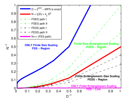
Figure 4: (Color online). Classification of MPS simulations of spin chains according to the simulation parameter pair $\{N,D\}$. All lines ending in the origin denote possible paths to approach the thermodynamic limit of critical systems when doing MPS simulations.

Now in general, there is a huge regime where for example $\Delta_{N}^{2}\ll\Delta_{D}\leq\Delta_{N}$ or $\Delta_{D}^{2}\ll\Delta_{N}\leq\Delta_{D}$. In this case the leading scaling behavior is modified by corrections that are not proportional to the next power of the relevant variable but to the ratio among the two variables. Indeed if we consider the scenario where $\Delta_{D}^{2}\ll\Delta_{N}\leq\Delta_{D}$ in Eq. 12 we obtain

$$f_{\Delta_{D},\Delta_{N}}=f_{0,0}+\Delta_{D}\left(\partial_{\Delta_{D}}f_{00}+\partial_{\Delta_{N}}f_{00}\frac{\Delta_{N}}{\Delta_{D}}\right)+\cdots$$ (13)

How relevant the correction is clearly depends on the scale separation, i.e. on how close $\Delta_{N}/\Delta_{D}$ is to one. In the following we give a sketch of how this cross-over region looks like and we introduce two new terms: Finite Entanglement-Size Scaling (FESS for) the region where the leading scaling is due to the finite size of the matrices and the corrections come from the size of the system and Finite Size-Entanglement Scaling (FSES) where the leading scaling is due to the size of the system and the corrections come from the size of the matrices.

Figure 4 shows a classification of MPS simulations according to the simulation parameter pair $\{N,D\}$. The thermodynamical limit can be approached by moving along any path towards the origin of the diagram $\{N^{-1}=0,D^{-1}=0\}$. However in order not to distort the scaling analysis by mixing the different $N$ and $D$ related corrections, moving from one point to the next on the path should leave the ratio $\Delta_{N}/\Delta_{D}$ unchanged. This is equivalent to the requirement that any path is completely determined by the path constant $k=N/D^{\kappa}$.

We can distinguish three different regions and three important lines in Fig. 4 In the region above the blue line which is defined by $D=d^{N/2}$, the MPS bond dimension is large enough to represent the ground state exactly. Of course doing MPS simulations in this regime is pointless since the computational cost becomes exponential in $N$ and there is no advantage over exact diagonalization. Thus no matter which path towards $N\to\infty$ we choose in this region, it is completely equivalent to FSS. The magenta line with $N^{-1}=0$ represents the only path along which pure finite entanglement scaling (FES) holds. The red line represents the path along which the induced correlation length is equal to the system size, i.e. $N=\xi(D)$. We will call this line in the following the critical line. For critical models without conformal invariance the critical line can be obtained using the method described in appendix A. Between this line and the FES line there is a region where $N>\xi(D)$. All simulations done in this region barely registrate the boundaries of the system and the fixed point MPS is more or less the same like that of a $N=\infty$ simulation with same $D$. However there is a slight effect due to the finite size for points close to the $N=\xi(D)$ line as can be seen in Figure 1. This is why we call this region the finite entanglement-size scaling (FESS) region: the entanglement scaling predominates, but there is a small trace of finite size scaling behavior. The region between the critical line and the FSS-regime describes MPS simulations where $\xi(D)<N$, which turn out to reproduce faithfully the long range correlations throughout the entire chain (see figure 9 in our previous work Pirvu et al. (2011)). The FSS aspect predominates in this region, however there is also the inherent error of MPS simulations with $D<d^{N/2}$, so we call it the finite size-entanglement scaling (FSES) region.

Despite the rigorous classification of regimes from Figure 4 we will restrict ourselves in the following to discriminate merely between the regimes on different sides of the critical line. We do this in order to improve the readability. Thus we will refer to both FSS and FSES as FSS; analogously we will denote both FES and FESS as FES.

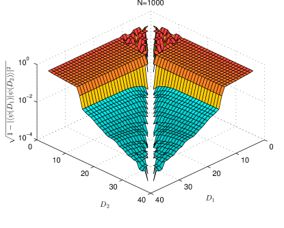
a) b)

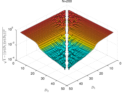
Figure 5: a) (Color online). Quantum Ising model: trace distance between ground state MPS with different bond dimensions $D_{1}$ and $D_{2}$ for a chain with $N=1000$ sites. b) Heisenberg model: trace distance between ground state MPS with different bond dimensions $D_{1}$ and $D_{2}$ for a chain with $N=200$ sites. By using relatively small bond dimensions we are able to localize the transition between the FES and FSS regime for each $N$. This can be used in case we are interested in performing a FSS analisys by providing the lower bound $D_{r}$ such that the state we obtain is not orthogonal to the exact state.

II.3 Minimal $D$ for faithful simulations

We can outline a direct application of the presence of a transition between a FSS regime and a FES regime. Suppose that we want to simulate a critical chain with PBC such that it is in the FSS regime, i.e. the properties due to the boundary conditions are faithfully reproduced since $N<\xi(D)$. In order to minimize the computational cost we would like to use the smallest possible $D$ that captures the PBC topology. By looking at figure 3 it is clear that we would have to choose $D=D_{r}$ to this end. The problem is that in order to make that plot we had to use as reference states MPS with very large $D=64$, which is exactly what we would like to avoid in this case. Fortunately it turns out that even without a large $D$ simulation it is possible to detect the optimal $D=D_{r}$. This is due to the fact that all MPS with $D\geq D_{r}$ have a much smaller trace distance among eachother than with MPS with $D<D_{r}$.

The trace distance among all states with $D<40$ for a IS chain with $N=1000$ is shown in figure 5 a). The plot is of course symmetric in $D_{1}$ and $D_{2}$ and we have omitted the points on the diagonal since they are trivially $0$. The transition between the FSS and the FES regime is clearly distinguishable at the same location of the jump as in figure 3 but in this plot we used only MPS with relatively small bond dimension. Note furthermore that if $D_{1},D_{2}<D_{r}$ the trace distance between these states is wildly oscillating. However if $D_{1}$ and $D_{2}$ are on different sides of the jump, profiles similar to figure 3 emerge. Now it is clear how we can find the optimal $D=D_{r}$ with the smallest computational cost possible: for a given $N$ run the PBC simulations by increasing $D$ in small steps, ideally $\Delta D=1$. After each simulation compute the overlap with all previously obtained MPS and when the nice profile with the jump appears, we know we have reached $D=D_{r}$. The same strategy can be employed for the HB model, however, just like in figure 3, the transition is much smoother in this case.

As a side remark note that due to the fast decay of the eigenvalues of the MPS transfer matrix one can compute the overlaps with computational cost scaling like $O(nD^{3})$. The meaning of $n$ and the method how to achieve this is described in Pirvu et al. (2011).

II.4 Thermodynamic limit of the transition

What can figure 3 tell us about the behavior of the transition between the FSS and FES in the limit $N\to\infty$?

For the IS model, qualitatively the height of the jump seems to remain constant for increasing $N$. The trace distance between MPS with bond dimensions $D_{l}$ and $D_{r}$ to the reference state also seems to remain more or less stable but this is of course not enough evidence for the persistence of the transition in the thermodynamic limit. In appendix B, we present a detailed analysis that shows that for the IS model i) the $N\to\infty$ limit of the trace distance between the exact ground state (approximated by a reference state) and MPS obtained in the FSS regime is strictly bigger than zero, ii) the same limit for the trace distance with respect to MPS obtained in the FES regime is zero. ii) implies that states in the FES regime are globally orthogonal to the exact ground state of the PBC chain. As we already mentioned above this does not affect the possibility to extract local universal information from those states. However ii) clearly shows that MPS in the FES regime are globally not a good approximation for the ground state of the IS model with PBC.

Unfortunately we cannot obtain the same conclusions for the HB model. Presumably this is due to the fact that the reference states that we use are not a good enough approximation of the true ground state of the model in this case. This becomes clear if we look again at figure 1: for the IS model the $D=64$ states have a much better precision than the MPS we compared them to in order to prove the persistence of the transition in the thermodynamic limit (see Appendix B for details). For the HB model on the other hand, the $D=64$ line covers almost three orders of magnitude in the relative precision plot; at its maximum it is over one order of magnitude above the points belonging to MPS that we must compare the reference states to in order to perform our analysis of the thermodynamic limit (e.g. the data points with $N=100$ and $D=48$). The $D=128$ line in right plot of figure 1 seems to fulfill similar requirements like the $D=64$ line in the left plot. However, in that regime, for $N\ll\xi(D)$, the PBC algorithm is very inefficient and it would take unreasonably long to obtain the data points for $D=128$.

II.5 The scaling function

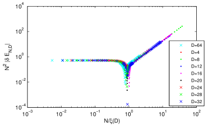
a) b)

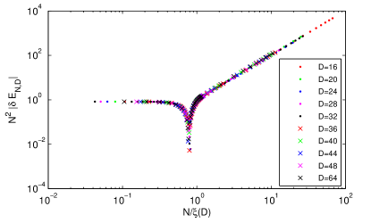
Figure 6: (Color online). a) Quantum Ising model: log-log plot of $N^{2}\lvert\delta E_{N,D}\rvert$ versus $N/\xi(D)$ that illustrates the collapse of the data into a single curve. The points with $D=64$ slightly deviate from the curve traced by data points with smaller $D$. b) Heisenberg model: log-log plot of $N^{2}\lvert\delta E_{N,D}\rvert$ versus $N/\xi(D)$ that illustrates the collapse of the data into a single curve.

Finally we conduct an analysis of the scaling of MPS simulations across the entire interval $N/\xi(D)\in(0,\infty)$ which covers all possible pairs $\{N,D\}$. This is very much in the spirit of the scaling analysis performed by Nishino et al. for classical 2D systems in Ref. Nishino et al. (1996). The main differences are that in our case the energy difference $\delta E_{N,D}$ can take both positive and negative values, and that we obtain the effective correlation length $\xi(D)$ from an analysis of the humps in the relative precision of the energy (see Appendix A for details) instead of using the ratio between the two biggest eigenvalues of the MPS transfer matrix.

Analogously to Nishino, we first eliminate the FSS scaling from $\lvert\delta E_{N,D}\rvert$ and then we plot the result (in our case this is $N^{2}\lvert\delta E_{N,D}\rvert$) as a function of $N/\xi(D)$. The fact that all data (with exception of the $D=64$ points for the IS model) collapses into a single curve justifies the assumption that

$$\delta E_{N,D}=E_{0}(N,D)-E_{0}(\infty)=\frac{f(N/\xi(D))}{N^{2}}\,\,\,.$$ (14)

with some scaling function $f(x)$ that is not exactly known. What we can easily write down however is its asymptotic behavior

$$\begin{split}\lim_{x\to 0}f(x)&=-\frac{v_{f}\pi c}{6}\\ \lim_{x\to\infty}f(x)&=\Delta\cdot\Big{(}\frac{N}{D^{\kappa}}\Big{)}^{2}\,\,\,.\end{split}$$ (15)

For the IS model we have used for $\xi(D)$ the expression obtained from the hyperbola fit in Fig. 8 of the Appendix A, i.e. $\xi(D)=3.810\cdot D^{2.042}$. Note that in plot a) of the Fig. 6, the data for different $D$ collapses almost perfectly in the extremal regimes $N\ll\xi(D)$ and $N\gg\xi(D)$. There is a slight deviation of the $D=64$ curve that can be explained if we look at figure 1 in Pirvu et al. (2010) (there the $D=64$ data point also slightly deviates from the line that is traced by the points with $D<64$). In the regime where $N\approx\xi(D)$ the curves do not collapse so nicely which is a manifestation of the fact that the humps in Fig. 1 are so different for the IS model.

For the HB model we have used for the effective correlation length $\xi(D)=3.647\cdot D^{1.338}$ as obtained from the hyperbola fit in Fig. 8. Plot b) of Fig. 6 shows an almost perfect collapse even in the region $N\approx\xi(D)$. Presumably this is due to the fact that for the HB model the humps in Fig. 1 are much more similar among each other than in the case of the IS model.

III Conclusions

An accurate analysis of MPS simulations of critical spin chains with PBC reveals the appearance of two regimes. The FSS regime where the energy gap of the system is induced by the size of the system and the FES regime where an effective energy gap is induced by finite $D$. While in both regimes local universal quantities can be extracted by studying the scaling of the observable with respect to the relevant variable (the size of the system for the FSS or the size of the MPS matrices for the FES regime), we have shown that for the Quantum Ising model, states in the FES regime are orthogonal to the exact ground state in the thermodynamic limit. Intuitively this happens due to the fact that for MPS simulations in the in the FES regime, the induced correlation length is smaller than the system size and thus the MPS is not aware of the size of the system. Since in critical systems the boundary conditions strongly affect global properties of the system, this result seems quite natural.

Our results can be interpreted as a further benchmark for recently introduced algorithms that try to lower the computational cost of PBC simulations with MPS Pippan et al. (2010); Pirvu et al. (2011); Shi and Zhou (2009); Rossini et al. (2011) (see Appendix C). Here we provide strong hints that in order to correctly describe the ground state of a finite chain with PBC for critical systems, these algorithms should be used with care in order not to obtain wave functions that are orthogonal to the exact ones. What one would indeed interpret as the MPS tensor for a PBC chain, in some regime could turn out to be closer to the MPS tensor of an infinite OBC system.

However, considering that for OBC systems the approach to the thermodynamic limit is by no means slower than for PBC systems (for both the ground state energy converges to the thermodynamic limit as a function of the appropriate correlation length like $\xi^{-2}$), our results can be also used in a constructive way. In order to extract universal information about local operators, one is better off by using FES rather than FSS, since simulations in the FES regime have a much better scaling of the computational cost.

Things are more complex if one is interested in global observables, such as e.g. two point correlation functions at half chain length. For PBC systems the scaling analysis must be performed in this case on paths with constant $k=N/D^{\kappa}$ that lie completely in the FSS regime. The computationally least expensive such path is the one where for every given $N$, the MPS bond dimension $D$ is just big enough such that $\xi_{D}>\xi_{N}$. We have shown how that minimal $D$ can be found for any $N$ by looking at the overlap between MPS with increasing $D$ until the discrete transition between the FES and the FSS regime is detected. Regarding the scaling exponent $\kappa$, we have been able to numerically confirm the theoretically predicted values with an accuracy of approximately $0.4\%$ for both the Quantum Ising and the Heisenberg models. Furthermore we have shown in Appendix A.1 how the analytical expression for $\kappa$, originally derived in Pollmann et al. (2009), can be obtained in an alternative way.

Following Nishino’s analysis for 2D classical systems Nishino et al. (1996) we have shown that also for MPS simulations of 1D quantum systems the scaling of the MPS ground state energy in simulations with finite $N$ and $D$ obeys a two-parameter scaling function. Finding an analytical expression for this function is something that still has to be done.

A further interesting future line of research is to understand how to extract information about the operator content of the Conformal Field Theories related to the infrared behavior of the studied critical spin systems (that strongly depend on boundary conditions Blöte et al. (1986); Evenbly et al. (2010)) directly out of the MPS tensors.

IV Acknowledgements

We thank V. Murg, I. McCulloch, E. Rico, V. Eisler for valuable discussions. The TDVP computation was kindly performed by J. Haegeman. This work was supported by the FWF doctoral program Complex Quantum Systems (W1210) the FWF SFB project FoQuS, the ERC grant QUERG, and the ARC grants FF0668731 and DP0878830. We aknowledge the financial support of the Marie Curie project FP7-PEOPLE-2010-IIF “ENGAGES” 273524.

Appendix A Effective correlation length

A.1 Analytical results

Recently it has been shown numerically that any MPS simulation of an infinite spin chain leads to the emergence of an effective correlation length induced by the finite rank $D$ of the MPS matrices, even if the studied system is critical Tagliacozzo et al. (2008). In Ref. Pollmann et al. (2009) the authors relate the numerical observation that $\xi(D)\propto D^{\kappa}$ from Ref. Tagliacozzo et al. (2008) to analytical results on the spectrum of the MPS transfer matrix Calabrese and Lefevre (2008) and to well-known results from conformal field theory Blöte et al. (1986); Affleck (1986) in order to derive an analytical expression for the exponent $\kappa$. Here we derive the same results in a different way.

The starting point for our argument is the same like the one in Pollmann et al. (2009), namely that corrections to the exact ground state energy in the thermodynamic limit can have different origins. On one hand conformal invariance yields in the vicinity of the critical point (i.e. $\epsilon=|\lambda-\lambda_{crit}|/\lambda_{crit}\ll 1$) according to Refs. Blöte et al. (1986); Affleck (1986); Pollmann et al. (2009)

$$E_{0}(\xi_{\epsilon})=E_{0}(\infty)+\frac{A}{\xi_{\epsilon}^{2}}$$ (16)

where $A$ is a non-universal constant. On the other hand, MPS simulations with finite $D$ yield according to Refs. Tagliacozzo et al. (2008); Calabrese and Lefevre (2008); Pollmann et al. (2009)

$$E_{0}(\xi_{D})=E_{0}(\infty)+\frac{\beta}{\xi_{D}}P_{r}(b,D)$$ (17)

where $\beta$ is a non-universal constant, $P_{r}(b,D)$ is the residual probability due to the usage of finite $D$ and $b$ is related to the dominant eigenvalue of the reduced density matrix of the half-chain (see Refs. Calabrese and Lefevre (2008); Pollmann et al. (2009)). Now it has been observed that the usage of finite $D$ in MPS simulations close to the critical point leads to an effective shift of the critical point (see Fig. 2 in Tagliacozzo et al. (2008)). This observation led us to the idea of equating the corrections in Eqs. (16) and (17) and identifying $\xi_{\epsilon}$ with $\xi_{D}$. Together with the assumption $\xi_{D}=k_{c}\cdot D^{\kappa}$ this yields

$$P_{r}(b,D)=\frac{A}{\beta\cdot\xi_{D}}=A^{\prime}\cdot D^{-\kappa}$$ (18)

where we have collected all constants into $A^{\prime}=A/(k_{c}\cdot\beta)$.

In the large $D$ limit (required due to our assumption of working in the scaling limit), the residual probability reads according to Pollmann et al. (2009)

$$P_{r}(b,D)=\frac{2be^{-b}D}{\log D-2b}e^{-(\log D)^{2}/4b}$$ (19)

where

$$b=\frac{c}{12}\log\xi_{D}\approx\frac{c\kappa}{12}\log D$$ (20)

and $c$ denotes the central charge in the associated conformal field theory. Inserting (19) and (20) into (18) yields after several steps

$$\frac{c\kappa}{6-c\kappa}D^{-\frac{c\kappa}{12}-\frac{3}{c\kappa}+1}=A^{\prime}\cdot D^{-\kappa}\,\,\,.$$ (21)

Equating the exponents in (21) yields a quadratic equation for $\kappa$ with the solutions

$$\kappa_{\pm}=\frac{6}{c\cdot(1\pm\sqrt{\frac{12}{c}})}\,\,\,.$$ (22)

The physical root is the one that is positive for all values of $c$, i.e.

$$\kappa=\frac{6}{c\cdot(1+\sqrt{\frac{12}{c}})}$$ (23)

which is exactly the result obtained in Ref. Pollmann et al. (2009).

A.2 Numerical results

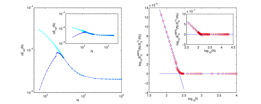
Figure 7: (Color online). Quantum Ising model data. Left: relative precision of the PBC-MPS ground state energy (blue/dark) and relative precision of the state used as an input for the PBC algorithm (i.e. obtained by inserting the TL-MPS, cyan/bright) as compared to the exact result for $D=8$ and $D=16$ (inset). Right: ratio between the PBC-MPS energy and the one of the input state (TL-MPS) for $D=8$ and $D=16$ (inset). Fitting a degenerate hyperbola in form of two straight lines yields a well defined point (the intersection point) whose value as a function of $D$ is proportional to the effective correlation length.

In this appendix we show how the effective correlation length $\xi(D)$ emerges in our simulations of finite spin chains with PBC. As the scaling of the algorithm Pirvu et al. (2011) is quasi-independent of the chain length $N$ we can use it to approximate ground states of arbitrary long chains with PBC. The relative precision of the MPS ground state energy for a given $D$ is plotted in figure 1 as a function of $N$. Each of the lines contains a hump which can be interpreted as the evidence for a finite correlation length $\xi(D)$. In order to see this let us have a look at how the hump emerges. The left part of figure 7 shows a comparison between the relative precision of the PBC-MPS ground state energy (i.e. the MPS towards which the algorithm in Pirvu et al. (2011) has converged) and the relative precision of the energy for the MPS that we had used as a starting point for the gradient search. As explained in Pirvu et al. (2011) this is the local MPS tensor obtained by imaginary time evolution Pirvu et al. (2010) for a chain in the thermodynamic limit (TL) when it is used in the finite PBC geometry. One can see that for a given $D$, on the left side of the hump there is considerable improvement in the precision of the energy between starting and ending point of the gradient search. As one approaches the hump from the left, the improvement decreases in order to vanish completely on the right side. This can be interpreted as follows: if $N$ is too large for a given $D$, the finite chain looks for a local MPS-tensor as if it would be infinite. Sites that lie further apart than a certain correlation length $\xi(D)$ effectively do not see each other. The transition to this region happens more or less smoothly since for growing powers of the MPS transfer matrix $T$, the subspace spanned by these powers gets smoothly restricted to the dominant eigenvector i.e. $T^{N}|_{N\gg\xi(D)}\approx\lambda_{1}^{N}\ket{\lambda_{1}}\bra{\lambda_{1}}$.

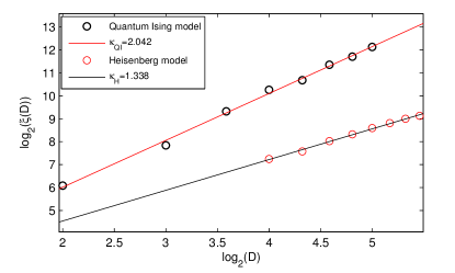
Figure 8: (Color online). Quantum Ising (upper) and Heisenberg model (lower): linear fit of the logarithm of the effective correlation length as a function of the bond dimension $D$.

Thus the humps must represent some evidence for the emergence of a finite correlation length, but how can we extract some reliable numbers from them, as they differ considerably in shape and width? The answer is given by the right part of figure 7. We have observed empirically that if we make a log-log plot of $E_{0}^{final}(N)/E_{0}^{initial}(N)$ we obtain approximately two straight lines connected by a small piece that is more or less smooth. This picture is reminiscent of a rotated hyperbola. We know furthermore that in the large $N$ limit all points have ordinate $0$. This suggests to fit a hyperbola that is degenerated to two straight lines through our data. The intersection of these lines is a well defined point which should be proportional to $\xi(D)$.

Figure 8 shows log-log plots of the effective correlation length as defined above for both the Quantum Ising and the Heisenberg models. After fitting straight lines through each of the data sets we can read off the scaling $\xi(D)=k_{c}\cdot D^{\kappa}$ with $\{\kappa\approx 2.042,k_{c}\approx 3.810\}_{IS}$ and $\{\kappa\approx 1.338,k_{c}\approx 3.647\}_{HB}$. Comparison with the analytical results (i.e. $\kappa_{IS}^{anal}\approx 2.03425$ and $\kappa_{HB}^{anal}\approx 1.34405$) yields a difference of roughly $0.4\%$ for the Quantum Ising model and of roughly $0.43\%$ for the Heisenberg model. These results are the ones we refer to in Sec. II.2 as the ones fulfilling $\xi(D_{l})<N<\xi(D_{r})$.

An alternative way to extract the effective correlation length is obtained by interpreting the abscissa of the minimum of each curve in Fig. 2 as a length proportional to $\xi(D)$. Fitting a straight line through these minima in a log-log plot of $N(D)$ yields for the IS model the exponent $\kappa_{\textrm{IS}}\approx 2.0293$ which approximates the analytical result with an accuracy of roughly $0.24\%$. On one hand this result is closer to the analytical value than the one obtained using the degenerated hyperbola fit. On the other hand, if we want to predict the bond dimension $D$ for which the jump in the trace distance occurs in simulations with fixed $N$, it turns out that the value obtained using this fit in does not always coincide with the actual values observed in figure 3. As mentioned above, the degenerated hyperbola fit satisfies this consistency test, which is why we prefer using that method to extract an approximation for $\kappa$. Furthermore the plots in figure 2 require knowledge of the exact ground state energy in the thermodynamic limit, which is not always available. The strategy with the hyperbola fit on the other hand does not require any analytical results and thus can always be used.

Appendix B Detailed treatment of the thermodynamic limit of the transition

In this appendix we present the details we used for the conclusion drawn in section II.4 of the main text. As mentioned above in appendix II.2.1 a reliable analysis of the thermodynamic limit can only be made properly if we move towards it on paths of constant $k=N/D^{\kappa}$. However this analysis provides conclusive results only for the IS model which is why we skip presenting the results obtained for the HB model. As mentioned in the main text, the reason why this method fails for the HB model is that the reference states are in that case not precise enough.

As a first step let us normalize the tensors in our states such that the largest eigenvalue of the MPS transfer matrix $T$ is equal to one (i.e. $\lambda_{1}=1$ and $\lambda_{i}\geq\lambda_{j},\,\,\,\forall i<j$). This yields for the norm of such a state

$$\braket{\Psi(D,N)}{\Psi(D,N)}=\mbox{Tr}(T^{N})=1+\sum_{i=2}^{D^{2}}\lambda_{i}^{N}(D,N)\,\,\,.$$ (24)

We will always use in the following lower-case greek letters to denote states that are normalized to one and upper-case letters for the corresponding state normalized according to (24), i.e.

$$\ket{\psi}=\frac{\ket{\Psi}}{\sqrt{\braket{\Psi}{\Psi}}}\,\,\,.$$ (25)

For the computation of the trace distance between reference states and states lying on a curve with fixed $k$ we need the absolute square of the overlap which becomes

$$\begin{split}&\left|\braket{\psi(D_{k,N},N)}{\psi(D_{\textrm{ref}},N)}\right|^{2}\\ =&\frac{\left|\braket{\Psi(D_{k,N},N)}{\Psi(D_{\textrm{ref}},N)}\right|^{2}}{\braket{\Psi(D_{k,N},N)}{\Psi(D_{k,N},N)}\braket{\Psi(D_{\textrm{ref}},N)}{\Psi(D_{\textrm{ref}},N)}}\\ =&\frac{\left[\sum_{i=1}^{D_{\textrm{ref}}\cdot D_{k,N}}\mu_{i}^{N}(D_{k,N},D_{\textrm{ref}},N)\right]^{2}}{\left[1+\sum_{i=2}^{D^{2}_{k,N}}\lambda_{i}^{N}(D_{k,N},N)\right]\left[1+\sum_{i=2}^{D_{\textrm{ref}}^{2}}\lambda_{i}^{N}(D_{\textrm{ref}},N)\right]}\,\,\,.\end{split}$$ (26)

In the numerator we have used $\mu_{i}(D_{k,N},D_{\textrm{ref}},N)=:\mu_{i}(k,N)$ to denote the eigenvalues of the overlap transfer matrix

$$T_{\textrm{ovlp}}(k,N)=\sum_{i=1}^{d}A_{i}(D_{k,N},N)\otimes A_{i}^{*}(D_{\textrm{ref}},N)\,\,\,,$$ (27)

where the $A_{i}(D,N)$ represent as usually the matrices of a translationally invariant MPS with $N$ sites and virtual bond dimension $D$. Similarly we will use for the eigenvalues of the MPS transfer matrix the notation $\lambda_{i}(k,N):=\lambda_{i}(D_{k,N},N)$ in the following. This can be done since we need only two of the quantities $(D,N,k)$ to uniquely specify the point of the phase diagram that we want to refer to.

The crucial argument in favor of the persistence of a discrete transition between the two regimes in the thermodynamic limit will be the fact that in this limit $\mu_{1}(k,N)$ converges much faster to $1$ in the FSS regime (i.e. for $k<k_{c}$) than it does in the FES regime (i.e. for $k>k_{c}$). In fact we will show below that in the first case $\lim_{N\to\infty}\mu_{1}^{N}(k,N)=1$ while in the second case we have $\lim_{N\to\infty}\mu_{1}^{N}(k,N)=0$. The other contributions in the numerator of (26) will turn out to be negligible for $N\to\infty$, i.e. $\lim_{N\to\infty}\mu_{i}^{N}(k,N)=0$ for any $k$ and all $i>1$. Furthermore we will show that the denominator of (26) remains finite in all cases such that we will be able to conclude that the overlap of the quasi-exact ground state with states in the FES regime converges to zero in the thermodynamic limit. Along the same lines we will argue that the overlap of the quasi-exact ground state with states in the FSES regime is always larger than zero in the thermodynamic limit, thereby concluding that a detectable transition between the two regimes persists for $N\to\infty$.

To this end we have considered three paths in the FSS regime ($k\approx{0.37,0.54,0.97}$) and two paths in the FES regime ($k\approx{18.0,58.7}$). The exact data points $(N,D)$ for four of these paths are listed in table 1. Note that since $N,D\in\mathbb{N}$ the exact value for $k=N/D^{\kappa}$ varies slightly within each path.

$\kappa=2.03425$
$k\approx 0.37<k_{c}$			$k\approx 0.54<k_{c}$			$k\approx 18.0>k_{c}$			$k\approx 58.7>k_{c}$
$k$	$N$	$D$	$k$	$N$	$D$	$k$	$N$	$D$	$k$	$N$	$D$
$0.374$	$122$	$17$	$0.538$	$118$	$14$	$17.9$	$300$	$4$	$58.9$	$1000$	$4$
$0.373$	$206$	$22$	$0.540$	$198$	$18$	$17.8$	$470$	$5$	$59.0$	$1580$	$5$
$0.371$	$288$	$26$	$0.540$	$298$	$22$	$18.3$	$700$	$6$	$58.7$	$2280$	$6$
$0.371$	$386$	$30$	$0.536$	$384$	$25$	$18.1$	$950$	$7$	$58.8$	$3130$	$7$
$0.369$	$526$	$35$	$0.539$	$560$	$30$	$18.2$	$1250$	$8$	$58.6$	$4100$	$8$
$0.369$	$690$	$40$	$0.537$	$810$	$36$	$17.7$	$1550$	$9$	$58.6$	$5210$	$9$
$0.368$	$1000$	$48$	$0.535$	$1000$	$40$	$18.0$	$1950$	$10$	$58.5$	$6450$	$10$
						$17.9$	$2350$	$11$	$58.4$	$7830$	$11$
						$17.9$	$2800$	$12$	$58.4$	$9350$	$12$

Table 1: Data points constituting several of the investigated paths with roughly constant $k$ depicted in figure 11.

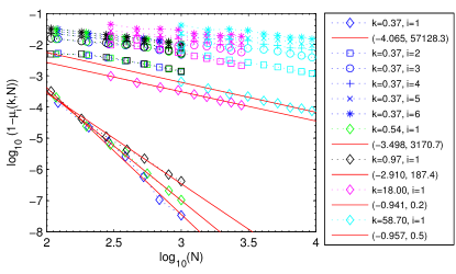
Figure 9: (Color online). Quantum Ising model: scaling of the eigenvalues of the overlap transfer matrix for five paths with roughly constant $k=N/D^{\kappa}$ in different regimes. The exact pairs $(N,D)$ for the data points are given in table 1. In the legend we have only explained in detail what the different markers mean for the path with $k\approx 0.37$. The markers for the other paths follow the same pattern. The full red lines are linear fits through the data for each $\mu_{1}(k,N)$ respectively. The legend entries for these lines contain the values $(-\beta_{1}(k),\alpha_{1}(k))$.

Let us first investigate how the numerator of the ratio (26) behaves. We have observed that if we look at the eigenvalues $\mu_{i}(k,N)$ along paths with constant $k$, then $1-\mu_{i}(k,N)$ scales polynomially in $N$ as can be seen in the log-log plot of figure 9, such that we have

$$\mu_{i}(k,N)=1-\frac{\alpha_{i}(k)}{N^{\beta_{i}(k)}}\,\,\,.$$ (28)

$\kappa=2.03425$
	$k\approx 0.37<k_{c}$		$k\approx 0.54<k_{c}$		$k\approx 0.97<k_{c}$
$i$	$\beta_{i}$	$\alpha_{i}$	$\beta_{i}$	$\alpha_{i}$	$\beta_{i}$	$\alpha_{i}$
$1$	$4.06477$	$57128.2$	$3.49773$	$3170.6$	$2.90998$	$187.3$
$2$	$0.66454$	$0.14622$	$0.64177$	$0.12814$	$0.60463$	$0.10416$
$3$	$0.51554$	$0.19106$	$0.51270$	$0.19112$	$0.48326$	$0.16400$
$4$	$0.58048$	$0.37486$	$0.57835$	$0.37607$	$0.55326$	$0.33117$
$5$	$0.48173$	$0.26650$	$0.51001$	$0.31294$	$0.51875$	$0.32733$
$6$	$0.50660$	$0.35546$	$0.50828$	$0.36216$	$0.49502$	$0.33813$
$7$	$0.47451$	$0.31883$	$0.46129$	$0.30227$	$0.42975$	$0.26069$
$8$	$0.46673$	$0.35474$	$0.46928$	$0.36415$	$0.45436$	$0.33884$
$9$	$0.48042$	$0.42354$	$0.47013$	$0.41012$	$0.44586$	$0.37264$
$10$	$0.51091$	$0.55418$	$0.50601$	$0.54819$	$0.48431$	$0.49597$

Table 2: Scaling of $\mu_{i}(k,N)$: parameters $\beta_{i}(k)$ and $\alpha_{i}(k)$ for the fitting of $1-\mu_{i}(k,N)=\alpha_{i}(k)/N^{\beta_{i}(k)}$ for paths in the FSES regime.

$\kappa=2.03425$
	$k\approx 18.0>k_{c}$		$k\approx 58.7>k_{c}$
$i$	$\beta_{i}$	$\alpha_{i}$	$\beta_{i}$	$\alpha_{i}$
$1$	$0.94079$	$0.20604$	$0.95736$	$0.46203$
$2$	$0.72904$	$0.74874$	$0.75036$	$1.14015$
$3$	$0.46762$	$0.25046$	$0.43380$	$0.23299$
$4$	$0.42154$	$0.26209$	$0.49195$	$0.62481$
$5$	$0.37208$	$0.23363$	$0.37851$	$0.33497$
$6$	$0.38713$	$0.38566$	$0.44232$	$0.87896$
$7$	$0.36770$	$0.38856$	$0.38792$	$0.65807$
$8$	$0.40633$	$0.58072$	$0.41378$	$0.94025$
$9$	$0.42088$	$0.80086$	$0.45836$	$1.67698$
$10$	$0.40215$	$0.80529$	$0.43306$	$1.58778$

Table 3: Scaling of $\mu_{i}(k,N)$: parameters $\beta_{i}(k)$ and $\alpha_{i}(k)$ for the fitting of $1-\mu_{i}(k,N)=\alpha_{i}(k)/N^{\beta_{i}(k)}$ for paths in the FESS regime.

Figure 9 shows a log-log plot of $1-\mu_{i}(k,N)$ for all $k$ and fixed $D_{ref}=64$. The numerical values of $\alpha_{i}(k)$ and $\beta_{i}(k)$ for the $10$ largest $\mu_{i}(k,N)$ are listed for the paths in the FES regime in table 2. The equivalent data for paths in the FES regime can be found in table 3. We see that in the FSS regime for $i=1$ we have $\beta_{1}(k)>1$ while in all other cases we get $\beta_{i}(k)<1$. This means that for $N\to\infty$ the overlap (26) always converges to zero in the FES regime due to

$$\lim_{N\to\infty}(1-\frac{\alpha}{N^{\beta}})^{N}=0\,\,\,\,\,\,\forall\beta<1,\alpha>0$$ (29)

and due to the fact that the denominator is always larger than zero (in fact it is always larger than one). In the FSS regime on the other hand, the $i=1$ terms in the numerator of (26) survive in the thermodynamic limit due to

$$\lim_{N\to\infty}(1-\frac{\alpha}{N^{\beta}})^{N}=1\,\,\,\,\,\,\forall\beta>1,\alpha>0\,\,\,.$$ (30)

However this is not enough in order to show that the overlap is strictly larger than zero in this regime. A diverging denominator in the limit $N\to\infty$ could spoil this line of reasoning, so we have to convince ourselves that both factors in the denominator of (26) remain finite in the thermodynamic limit.

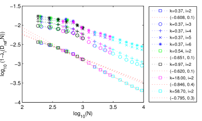
Figure 10: (Color online). Quantum Ising model: scaling of the eigenvalues of the MPS transfer matrix for $D_{\textrm{ref}}=64$ and all $N$ occuring in table 1. In the legend we have only explained in detail what the different markers mean for the $N$ in the path with $k\approx 0.37$. The markers for the other paths follow the same pattern. The dotted red lines are linear fits through the data for each $\lambda_{2}(k,N)$ respectively. The legend entries for these lines contain the values $(-\beta_{2}(k),\alpha_{2}(k))$.

$\kappa=2.03425$
	$k\approx 0.37<k_{c}$		$k\approx 0.54<k_{c}$		$k\approx 0.97<k_{c}$
$i$	$\beta_{i}$	$\alpha_{i}$	$\beta_{i}$	$\alpha_{i}$	$\beta_{i}$	$\alpha_{i}$
$2$	$0.60788$	$0.09304$	$0.65085$	$0.12184$	$0.62045$	$0.09914$
$3$	$0.41227$	$0.08847$	$0.46692$	$0.12433$	$0.44144$	$0.10401$
$4$	$0.43118$	$0.12846$	$0.48404$	$0.17837$	$0.45909$	$0.14987$
$5$	$0.30225$	$0.07647$	$0.36915$	$0.11385$	$0.35609$	$0.10226$
$6$	$0.34175$	$0.10783$	$0.40765$	$0.15889$	$0.39654$	$0.14462$
$7$	$0.40046$	$0.17074$	$0.44681$	$0.22606$	$0.43958$	$0.21126$
$8$	$0.41688$	$0.19910$	$0.46402$	$0.26460$	$0.45243$	$0.24089$
$9$	$0.33412$	$0.13003$	$0.36584$	$0.15862$	$0.36051$	$0.15116$
$10$	$0.28957$	$0.10620$	$0.34067$	$0.14540$	$0.33743$	$0.14045$

Table 4: Scaling of $\lambda_{i}(D_{\textrm{ref}},k,N)$: parameters $\beta_{i}(k)$ and $\alpha_{i}(k)$ for the fitting of $1-\lambda_{i}(D_{\textrm{ref}},k,N)=\alpha_{i}(k)/N^{\beta_{i}(k)}$ for paths in the FSES regime.

$\kappa=2.03425$
	$k\approx 18.0>k_{c}$		$k\approx 58.7>k_{c}$
$i$	$\beta_{i}$	$\alpha_{i}$	$\beta_{i}$	$\alpha_{i}$
$2$	$0.84555$	$0.42728$	$0.79472$	$0.28481$
$3$	$0.76096$	$0.82750$	$0.67333$	$0.41376$
$4$	$0.76823$	$1.11696$	$0.68922$	$0.59758$
$5$	$0.61161$	$0.54136$	$0.51839$	$0.26161$
$6$	$0.55554$	$0.41101$	$0.49502$	$0.25624$
$7$	$0.42416$	$0.19075$	$0.52876$	$0.42488$
$8$	$0.36840$	$0.13854$	$0.42626$	$0.21306$
$9$	$0.42172$	$0.22169$	$0.40383$	$0.19455$
$10$	$0.39138$	$0.19807$	$0.31502$	$0.10918$

Table 5: Scaling of $\lambda_{i}(D_{\textrm{ref}},k,N)$: parameters $\beta_{i}(k)$ and $\alpha_{i}(k)$ for the fitting of $1-\lambda_{i}(D_{\textrm{ref}},k,N)=\alpha_{i}(k)/N^{\beta_{i}(k)}$ for paths in the FESS regime.

Let us first treat the norm of the reference MPS since this turns out to be the easier one. Figure 10 shows a log-log plot of $1-\lambda_{i}(k,N)$ for all $k$ and fixed $D_{ref}=64$. The numerical values for $i\leq 10$ are given in tables 4 and 5. For large chains with $N>1000$ figure 10 clearly indicates polynomial scaling in $N$. Note that for small chains with $N<1000$ the plot deviates from the nice linear behavior that we see for $N>1000$. The reason for this are numerical errors in the computation of the ground state MPS. This effect can also be seen in figure 1: for $N<1000$ the algorithm we use cannot minimze the energy beyond a relative precision of roughly $8\cdot 10^{-11}$ even if we decrease $N$ while keeping a constant $D=64$. Apart from that, the fitting in figure 10 yields all $\beta_{i}(k)<1$ for $i\geq 2$ thus we can conclude that the norm $\braket{\Psi(D_{ref},N)}{\Psi(D_{ref},N)}$ converges to one in the thermodynamic limit when we use the normalization prescription (24).

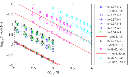
Figure 11: (Color online). Quantum Ising model: scaling of the eigenvalues of the MPS transfer matrix for five paths with roughly constant $k=N/D^{\kappa}$ in different regimes. The exact pairs $(N,D)$ for the data points are given in table 1. In the legend we have only explained in detail what the different markers mean for the path with $k\approx 0.37$. The markers for the other paths follow the same pattern. The full red lines are linear fits through the data for each $\lambda_{2}(k,N)$ respectively. The legend entries for these lines contain the values $(-\beta_{2}(k),\alpha_{2}(k))$.

$\kappa=2.03425$
	$k\approx 0.37<k_{c}$		$k\approx 0.54<k_{c}$		$k\approx 0.97<k_{c}$
$i$	$\beta_{i}$	$\alpha_{i}$	$\beta_{i}$	$\alpha_{i}$	$\beta_{i}$	$\alpha_{i}$
$2$	$0.99979$	$1.36876$	$0.99261$	$1.37029$	$0.98869$	$1.45137$
$3$	$0.99838$	$5.00085$	$0.98501$	$4.96160$	$0.97751$	$5.42433$
$4$	$0.99397$	$6.19275$	$0.98129$	$6.13836$	$0.97395$	$6.67115$
$5$	$1.00992$	$11.36417$	$0.97979$	$10.64645$	$0.96439$	$11.79694$
$6$	$0.99749$	$12.14274$	$0.96755$	$11.35451$	$0.95325$	$12.79517$
$7$	$0.99290$	$15.20975$	$0.96478$	$14.29878$	$0.94933$	$15.72285$
$8$	$0.99385$	$16.84721$	$0.94982$	$14.52223$	$0.93257$	$16.11736$
$9$	$1.03853$	$23.13857$	$0.98133$	$19.63216$	$0.94593$	$20.59742$
$10$	$1.03720$	$25.64027$	$0.95765$	$19.24667$	$0.92658$	$21.15268$

Table 6: Scaling of $\lambda_{i}(k,N)$: parameters $\beta_{i}(k)$ and $\alpha_{i}(k)$ for the fitting of $1-\lambda_{i}(k,N)=\alpha_{i}(k)/N^{\beta_{i}(k)}$ for paths in the FSES regime.

$\kappa=2.03425$
	$k\approx 18.0>k_{c}$		$k\approx 58.7>k_{c}$
$i$	$\beta_{i}$	$\alpha_{i}$	$\beta_{i}$	$\alpha_{i}$
$2$	$1.01831$	$40.25148$	$1.01731$	$135.41657$
$3$	$0.98774$	$81.55159$	$0.98683$	$264.69533$
$4$	$0.97128$	$88.78991$	$0.97053$	$282.91558$
$5$	$0.92704$	$111.61975$	$0.92647$	$337.75755$
$6$	$0.88126$	$94.42375$	$0.88080$	$270.69784$
$7$	$0.88252$	$104.24989$	$0.88232$	$299.97710$
$8$	$0.77072$	$64.57797$	$0.77072$	$162.76623$
$9$	$0.79065$	$82.78179$	$0.78996$	$212.48337$
$10$	$0.76184$	$72.53475$	$0.76185$	$180.90762$

Table 7: Scaling of $\lambda_{i}(k,N)$: parameters $\beta_{i}(k)$ and $\alpha_{i}(k)$ for the fitting of $1-\lambda_{i}(k,N)=\alpha_{i}(k)/N^{\beta_{i}(k)}$ for paths in the FESS regime.

The norm of the states $\ket{\Psi(D_{k,N},N)}$ along paths with constant $k$ also turns out to converge to a finite value even though the argument is a bit trickier in this case. The scaling of the largest eigenvalues $\lambda_{i}(k,N)$ for each path is shown in figure 11. The numerical values for $i\leq 10$ are given in tables 6 and 7. We see that most of the $\beta_{i}(k)$ are very close to one for small $i$ in contrast to the values obtained for $\lambda_{i}(D_{ref},N)$ which are all well below one. In fact some of the $\beta_{i}(k)$ are even bigger than one suggesting that $\lim_{N\to\infty}\lambda_{i}^{N}=1$ in these cases. In section B.1 of this appendix we give evidence for the fact that even if $\beta_{i}(k)>1$ in some cases, the number of these values remains finite for any $k$. Furthermore we argue that in these cases it is reasonable to assume that we actually have $\beta_{i}(k)=1$ which yields in the thermodynamic limit

$$\lim_{N\to\infty}\lambda_{i}^{N}(k,N)=\lim_{N\to\infty}(1-\frac{\alpha_{i}}{N})^{N}=\exp(-\alpha_{i})\,\,\,.$$ (31)

Summing up all relevant contributions then yields for the norm of states in the different regimes

$$\begin{split}\lim_{N\to\infty}\braket{\Psi(k,N)}{\Psi(k,N)}_{k<k_{c}}&\approx 2.2\\ \lim_{N\to\infty}\braket{\Psi(k,N)}{\Psi(k,N)}_{k>k_{c}}&\leq 2.0\,\,\,.\end{split}$$ (32)

This allows us to approximate the overlap (with a quasi-exact state) towards which MPS simulations in different regimes converge to (on the paths we considered) as

$$\begin{split}\lim_{N\to\infty}\braket{\psi(k,N)}{\psi(D_{\textrm{ref}},N)}_{k<k_{c}}&\approx 0.45\\ \lim_{N\to\infty}\braket{\psi(k,N)}{\psi(D_{\textrm{ref}},N)}_{k>k_{c}}&=0\,\,\,.\end{split}$$ (33)

Thus we can conclude that the thermodynamic limit of the overlap in the FSS regime is always greater than zero proving that there is indeed an discrete transition from the FSS regime to the FES regime where the overlap becomes zero.

B.1 Scaling of $\lambda_{i}(k,N)$

The first ten parameters $\alpha_{i}$ and $\beta_{i}$ for the MPS transfer matrix eigenvalues $\lambda_{i}(k,N)$ on paths in the FSES regime are given in table 6, the ones for paths in the FESS regime in table 7. In the FESS regime we have $\beta_{2}>1$ which then yields a contribution of $\lim_{N\to\infty}\lambda_{2}^{N}(k)=1$ to the norm. For $i>2$ we clearly see how the $\beta_{i}$ rapidly decay below one, thereby making sure that the corresponding contributions to the norm become zero in the thermodynamic limit. This means that if we approach the thermodynamic limit on paths in the FESS regime and always normalize the MPS according to (24), i.e. $\lambda_{1}=1$, the norm of these states does not get bigger than two. In fact it is very likely that the true contribution of $\lambda_{2}$ is de facto zero : for $N$ as big as $10^{9}$, using the values for $\alpha_{2}$ and $\beta_{2}$ given in table 7, we get $\lambda_{2}^{N}(k=18.0)\approx 2\cdot 10^{-12}$ and $\lambda_{2}^{N}(k=58.7)\approx 4\cdot 10^{-42}$.

In the FSES regime on the other hand the $\beta_{i}$ seem to oscillate randomly around one so we must look at the behavior of larger $i$ in order to see if and when they decay below one, which is what we ultimately need in order to show that the norm of these states remains finite in the thermodynamic limit when the normalization prescription (24) is employed.

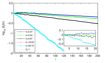
Figure 12: (Color online). Quantum Ising model: log-plot of the first values of $\beta_{i}(k)$ for $i\leq 200$. A zoomed view on the first $20$ values is shown in the inset.

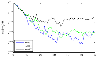
Figure 13: (Color online). Quantum Ising model: contribution of the eigenvalues with $\beta_{i}(k)\approx 1$ to the norm of the states in the thermodynamic limit, i.e. $\lim_{N\to\infty}\lambda_{i}^{N}(k)\approx\exp(-\alpha_{i}(k))$. Note how all contributions fall off exponentially below machine precision at $i\approx 14$.

Figure 12 shows a log-plot of the first $200$ $\beta_{i}$ in the FSES regime and of the first $120$ in the FESS regime. All curves are approximately straight lines in this plot which means that the $\beta_{i}$ decay exponentially with $i$. Remember that on the paths we chose to investigate in the FESS regime, the MPS with the largest virtual bond dimension have $D=12$, thus we cannot fit any parameters $\beta_{i}$ for $i>121$ since we have only one data point available there. For $100<i\leq 121$ we have only two data points, namely the ones for $D=11$ and $D=12$ (see table 1 in the main text) which is usually not the best premise for an accurate fit. Nonetheless the $\beta_{i}$ fitted in this range obey the same exponential decay observed for smaller $i$, where more data points are available. The inset in figure 12 shows a zoom into the region with $i\leq 20$. While for $i\leq 8$ all $\beta_{i}$ in the FSES regime are very close to one, we observe that for larger $i$, the $k=0.37$ line is visibly above the $\beta_{i}=1$ line. This would suggest that in the thermodynamic limit the eigenvalues $\lambda_{i>8}$ would each yield a contribution equal to one to the norm while the contribution from the $\lambda_{i}$ with $i\in\{2,3,4,6,7,8\}$ would vanish, since in these cases $\beta_{i}<1$. This makes however no sense since the $\lambda_{i}$ are decreasingly ordered, i.e. $\lambda_{i}>\lambda_{j}$ if $i<j$. This leads us to the conclusion that the oscillations around one that we observe for $i>8$ are numerical relics and that the true value of the $\beta_{i}$ is either one or something smaller than one. This conclusion is based on the fact that in MPS simulations the transfer matrix eigenvalues that converge first are the dominant eigenvalues (i.e. the ones with the largest absolute value) so we can assume that the values obtained for $\beta_{i\leq 8}$ are much more accurate than the other ones.

Thus the worst case for our purpose is when all $\beta_{i}$ that are not clearly smaller than one, are actually equal to one. Let us investigate what we would get for the norm in this case. If $\beta_{i}=1$, the contribution of these eigenvalues to the norm in the thermodynamic limit solely depends on $\alpha_{i}$ due to

$$\lim_{N\to\infty}\lambda_{i}^{N}(k,N)=1\lim_{N\to\infty}(1-\frac{\alpha_{i}}{N})^{N}=\exp(-\alpha_{i})\,\,\,.$$ (34)

Figure 13 shows the behavior of $\exp(-\alpha_{i})$ for the paths in the FSES regime and $i<60$, which according to figure 12 is the problematic $i$-range. We see how all contributions rapidly decay below machine precision. Note that the black line (i.e. the path with $k=0.97$) is for $i\geq 17$ several orders of magnitude above the $k=0.37$ and $k=0.54$ lines, which is due to the fact that the corresponding $\beta_{i}$ are so much smaller than one in this region, that the assumption $\beta_{i}\approx 1$ simply does not hold, and the actual contribution to the norm converges to zero. Note furthermore how for small $i$ all three lines are almost on top of each other meaning that the values to which the norm converges in the thermodynamic limit for MPS on different paths in the FSES regime will be very similar. In fact we get

$$\begin{split}\lim_{N\to\infty}\braket{\Psi(k,N)}{\Psi(k,N)}_{k=0.37}&=2.261646939734277\\ \lim_{N\to\infty}\braket{\Psi(k,N)}{\Psi(k,N)}_{k=0.54}&=2.236037631274709\\ \lim_{N\to\infty}\braket{\Psi(k,N)}{\Psi(k,N)}_{k=0.97}&=2.225635928039641\\ \end{split}$$ (35)

which completes our argument that the norm of the MPS remains finite on any path in the FSES regime.

Appendix C Comparison to other PBC MPS algorithms

In this appendix we will show that the algorithm Pirvu et al. (2011) that we used to obtain all results in this work is performing better than other recently presented approaches.

For the sake of completeness let us first recapitulate the result of the comparison to the algorithm presented in Pippan et al. (2010). We have already shown in Pirvu et al. (2011) that our PBC algorithm yields a better precision. Apart from several other differences in these two approaches, the crucial point is that we allow for a variable dimension $n$ of the dominant subspace used to approximate big powers of the transfer matrix. Even though this contributes a factor $n^{2}$ to the overall computational cost $O(n^{2}D^{3})$, we have shown in Pirvu et al. (2011) that there is no way to get rid of the factor $n$ if one wants to reproduce the correlation function throughout the entire PBC chain faithfully. If the same $n$-scanning strategy would be employed in Pippan et al. (2010), probably the same precision level could be achieved, however the computational cost in that algorithm would then scale like $O(NnD^{3})$. There is an additional factor $N$ in that scaling because that approach is not translationally invariant. The power of $n$ is reduced by one due to the fact that the energy is minimized directly and not using the gradient.

Next we would like to compare our PBC algorithm to the one presented in Shi and Zhou (2009). In that work the authors simulate the critical Quantum Ising Model by using Time Evolving Block Decimation Vidal (2004) to locally update a translationally invariant MPS which is then plugged into a chain with PBC geometry in order to compute the energy. The weakness of that algorithm is that the local update of the MPS tensors does not take into account the boundary conditions: the fixed point MPS is exactly the same like the one obtained when trying to approximate the ground state of an infinite chain. In spite of this, the ground state energy can be approximated quite well since the scaling of the computational cost is only $O(nD^{3})$ which allows the use of very large $D$. Unfortunately there are no explicit plots of the precision of the ground state energy in Shi and Zhou (2009) as a function of $D$. From the abstract and footnote 4 of that work we deduce that the simulation that yields the error $\approx 2.0\times 10^{-10}$ for the critical Quantum Ising PBC chain with $N=4800$ was done with a MPS with bond dimension $D=200$. We reach the same precision with $D$ as small as $64$ as can be seen in figure 1. Due to the higher computational cost of our algorithm $D=200$ is out of reach for us. Nonetheless we have computed an approximation of the ground state of the infinite chain with a translationally invariant MPS with $D=200$ (details of this are given below) and then plugged this MPS into a PBC chain geometry with $N=4800$. The relative precision that we obtained using this strategy was $\Delta_{rel}E_{0}(N=4800,D=200)\approx 1.39\cdot 10^{-10}$ which is in perfect agreement with the claim made in Shi and Zhou (2009). However, if we take into account the fact that a PBC simulation with $N=4800$ and $D=200$ is well in the FSES regime due to $N\ll\xi(D=200)\approx 1.910^{5}$, it becomes immediately clear that with $D=200$ one can in principle reach a much better precision than $\approx 10^{-10}$. In other words, the results obtained in Shi and Zhou (2009) correspond to the cyan (light) lines in the left plot of figure 7. While this is perfectly fine for simulations in the FESS regime, if one is in the FSES regime, there is room for one or more orders of magnitude of improvement of the relative precision.

There is another point worth mentioning regarding our PBC algorithm Pirvu et al. (2011). In order to check the claims made in Shi and Zhou (2009), we needed to first approximate the ground state of the infinite chain with an MPS with $D=200$. For this we used a new method called Time-Dependent Variational Principle Haegeman et al. (2011). We did this because TDVP converges much faster than Imaginary Time Evolution based on Matrix Product Operators Pirvu et al. (2010) or iTEBD Vidal (2007). The relative precision we achieved with TDVP was $\Delta_{rel}E_{0}(N=\infty,D=200)\approx 7.7\cdot 10^{-11}$. We knew that this cannot be the best precision that can be reached with $D=200$ since in Pirvu et al. (2010) we get roughly the same precision with $D$ as small as $128$. Thus we ran the PBC algorithm for a huge chain with $N=10^{6}$ sites on top of the MPS obtained by TDVP. Choosing as the parameters of that algorithm $m=1000$ and $n=100$ we managed to reduce the relative precision to $\approx 1.3\cdot 10^{-11}$ which is in perfect agreement with the polynomial scaling shown in figure 1 of Pirvu et al. (2010). The lesson learned from this approach is that TDVP results can be improved using our PBC algorithm well in the FESS regime. We emphasize that running the PBC algorithm with small $n$ did not yield any improvement to the TDVP result. Only with $n$ as large as $100$ we obtained the improved precision. This is quite strange as when we compute the energy density for the infinite chain, only one dominant eigenvector is used, i.e. $n=1$. So it seems that even if additional dominant eigenvectors do not enter the final computation of the ground state energy, they do have an effect during the local optimization procedure of the translationally invariant MPS.

References

- Klümper et al. (1993) A. Klümper, A. Schadschneider, and J. Zittartz, EPL (Europhysics Letters) 24, 293 (1993), URL http://stacks.iop.org/0295-5075/24/i=4/a=010
- Verstraete et al. (2008) F. Verstraete, V. Murg, and J. Cirac, Advances in Physics 57, 143 (2008)
- Schollwöck (2011) U. Schollwöck, Annals of Physics 326, 96 (2011), ISSN 0003-4916
- Fannes et al. (1992) M. Fannes, B. Nachtergaele, and R. Werner, Communications in Mathematical Physics 144, 443 (1992), ISSN 0010-3616, 10.1007/BF02099178, URL http://dx.doi.org/10.1007/BF02099178
- Affleck et al. (1987) I. Affleck, T. Kennedy, E. H. Lieb, and H. Tasaki, Phys. Rev. Lett. 59, 799 (1987)
- Barber (1983) M. N. Barber, Phase Transitions and Critical Phenomena edited by C. Domb and J. L. Lebowitz Vol. 8. (Academic, New York, 1983)
- Tagliacozzo et al. (2008) L. Tagliacozzo, T. R. de Oliveira, S. Iblisdir, and J. I. Latorre, Phys. Rev. B 78, 024410 (2008)
- Not (a) Additionally, one can also deform the system by describing it on curved geometries where the curvature induces a gap, and then study the approach to the flat limit in the same way one would study the approach to an infinite system Ueda and Nishino (2009).
- Blöte et al. (1986) H. W. J. Blöte, J. L. Cardy, and M. P. Nightingale, Phys. Rev. Lett. 56, 742 (1986)
- Pollmann et al. (2009) F. Pollmann, S. Mukerjee, A. M. Turner, and J. E. Moore, Phys. Rev. Lett. 102, 255701 (2009)
- Zheng et al. (2011) D. Zheng, G. Zhang, T. Xiang, and D. Lee, Physical Review B 83, 014409 (2011), URL http://link.aps.org/doi/10.1103/PhysRevB.83.014409
- Rodríguez et al. (2011) K. Rodríguez, A. Argüelles, A. K. Kolezhuk, L. Santos, and T. Vekua, Physical Review Letters 106, 105302 (2011), URL http://link.aps.org/doi/10.1103/PhysRevLett.106.105302
- Dai et al. (2010) Y. Dai, B. Hu, J. Zhao, and H. Zhou, Journal of Physics A: Mathematical and Theoretical 43, 372001 (2010), ISSN 1751-8113, 1751-8121, URL http://iopscience.iop.org/1751-8113/43/37/372001
- Orus and Wei (2010) R. Orus and T. Wei (2010), URL http://adsabs.harvard.edu/abs/2010arXiv1006.5584O
- McCulloch (2008) I. P. McCulloch, arXiv:0804.2509 (2008), URL http://arxiv.org/abs/0804.2509
- Heidrich-Meisner et al. (2009) F. Heidrich-Meisner, I. P. McCulloch, and A. K. Kolezhuk, Physical Review B 80, 144417 (2009), URL http://link.aps.org/doi/10.1103/PhysRevB.80.144417
- Zhao et al. (2010) J. Zhao, H. Wang, B. Li, and H. Zhou, Physical Review E 82, 061127 (2010), URL http://link.aps.org/doi/10.1103/PhysRevE.82.061127
- Pirvu et al. (2011) B. Pirvu, F. Verstraete, and G. Vidal, Phys. Rev. B 83, 125104 (2011), eprint arXiv:1005.5195
- Verstraete et al. (2004) F. Verstraete, D. Porras, and J. I. Cirac, Phys. Rev. Lett. 93, 227205 (2004)
- Pippan et al. (2010) P. Pippan, S. R. White, and H. G. Evertz, Phys. Rev. B 81, 081103 (2010)
- Shi and Zhou (2009) Q.-Q. Shi and H.-Q. Zhou, Journal of Physics A: Mathematical and Theoretical 42, 272002 (2009)
- Rossini et al. (2011) D. Rossini, V. Giovannetti, and R. Fazio, Journal of Statistical Mechanics: Theory and Experiment 2011, P05021 (2011), URL http://stacks.iop.org/1742-5468/2011/i=05/a=P05021
- Not (b) Eigenvector corresponding to the eigenvalue with the largest magnitude.
- Cardy (1986) J. L. Cardy, Nuclear Physics B 270, 186 (1986), ISSN 0550-3213
- Liu et al. (2010) C. Liu, L. Wang, A. W. Sandvik, Y.-C. Su, and Y.-J. Kao, Phys. Rev. B 82, 060410 (2010), URL http://link.aps.org/doi/10.1103/PhysRevB.82.060410
- Evenbly et al. (2010) G. Evenbly, R. N. C. Pfeifer, V. Picó, S. Iblisdir, L. Tagliacozzo, I. P. McCulloch, and G. Vidal, Phys. Rev. B 82, 161107 (2010), URL http://link.aps.org/doi/10.1103/PhysRevB.82.161107
- Nishino et al. (1996) T. Nishino, K. Okunishi, and M. Kikuchi, Physics Letters A 213, 69 (1996), ISSN 0375-9601
- Affleck (1986) I. Affleck, Phys. Rev. Lett. 56, 746 (1986), URL http://link.aps.org/doi/10.1103/PhysRevLett.56.746
- Pirvu et al. (2010) B. Pirvu, V. Murg, J. I. Cirac, and F. Verstraete, New J. Phys. 12, 025012 (2010)
- Ueda and Nishino (2009) H. Ueda and T. Nishino, Journal of the Physical Society of Japan 78, 014001 (2009), ISSN 0031-9015, URL http://jpsj.ipap.jp/link?JPSJ/78/014001/
- Calabrese and Lefevre (2008) P. Calabrese and A. Lefevre, Phys. Rev. A 78, 032329 (2008)
- Not (c) is the energy of the MPS obtained as the ground state by our conjugate gradient search for the finite chain with sites and PBC. is the energy obtained by plugging the MPS resulting from imaginary time evolution of the infinite chain into the finite size geometry with PBC. As mentioned in the main text, this MPS is used as the starting point of the conjugate gradient search.
- Not (d) Quasi-exact means in this context that we use as a reference state a MPS with virtual bond dimension that is much larger than the one of the studied points on the path of constant . If we restrict our scaling analysis to chains of length it is sensible to assume that the MPS with bond dimension is much closer to the exact ground state than it is to the states we analyze. Thus the overlap that we obtain in this way is very close to the overlap with the exact ground state.
- Not (e) Actually it might also be that is in fact equal to one which yields in the thermodynamic limit . Unfortunately, as opposed to the similar case in the FSES regime, we cannot conclude here that this must be the case.
- Vidal (2004) G. Vidal, Phys. Rev. Lett. 93, 040502 (2004)
- Haegeman et al. (2011) J. Haegeman, J. Cirac, T. Osborne, I. Pizorn, H. Verschelde, and F. Verstraete (2011), eprint arXiv:1103.0936
- Vidal (2007) G. Vidal, Phys. Rev. Lett. 98, 070201 (2007)