Regularized Partial Least Squares with an Application to NMR Spectroscopy

Abstract

High-dimensional data common in genomics, proteomics, and chemometrics often contains complicated correlation structures. Recently, partial least squares (PLS) and Sparse PLS methods have gained attention in these areas as dimension reduction techniques in the context of supervised data analysis. We introduce a framework for Regularized PLS by solving a relaxation of the SIMPLS optimization problem with penalties on the PLS loadings vectors. Our approach enjoys many advantages including flexibility, general penalties, easy interpretation of results, and fast computation in high-dimensional settings. We also outline extensions of our methods leading to novel methods for Non-negative PLS and Generalized PLS, an adaption of PLS for structured data. We demonstrate the utility of our methods through simulations and a case study on proton Nuclear Magnetic Resonance (NMR) spectroscopy data.

Keywords: sparse PLS, sparse PCA, NMR spectroscopy, generalized PCA, non-negative PLS, generalized PLS

1 Introduction

Technologies to measure high-throughput biomedical data in proteomics, chemometrics, and genomics have led to a proliferation of high-dimensional data that pose many statistical challenges. As genes, proteins, and metabolites, are biologically interconnected, the variables in these data sets are often highly correlated. In this context, several have recently advocated using partial least squares (PLS) for dimension reduction of supervised data, or data with a response or labels (Nguyen and Rocke, 2002b; Boulesteix and Strimmer, 2007; Rossouw et al., 2008; Chun and Keleş, 2010). First introduced by Wold (1966) as a regression method that uses least squares on a set of derived inputs accounting for multi-colinearities, others have since proposed alternative methods for PLS with multiple responses (de Jong, 1993) and for classification (Marx, 1996; Barker and Rayens, 2003). More generally, PLS can be interpreted as a dimension reduction technique that finds projections of the data that maximize the covariance between the data and the response. Recently, several have proposed to encourage sparsity in these projections, or loadings vectors, to select relevant features in high-dimensional data (Rossouw et al., 2008; Chun and Keleş, 2010). In this paper, we seek a more general and flexible framework for regularizing the PLS loadings that is computationally efficient for high-dimensional data.

There are several motivations for regularizing the PLS loadings vectors. Partial least squares is closely related to principal components analysis (PCA); namely, the PLS loadings can be computed by solving a generalized eigenvalue problem (de Jong, 1993). Several have shown that the PCA projection vectors are asymptotically inconsistent in high-dimensional settings (Johnstone and Lu, 2009; Jung and Marron, 2009). This is also the case for the PLS loadings, recently shown in Nadler and Coifman (2005) and Chun and Keleş (2010). For PCA, encouraging sparsity in the loadings has been shown to yield consistent projections (Johnstone and Lu, 2009; Amini and Wainwright, 2009). While an analogous result has not yet been shown in the context of PLS, one could surmise that such a result could be attained. In fact, this is the motivation for Chun and Keleş (2010)’s recent Sparse PLS method. In addition to consistency motivations, sparsity has many other qualities to recommend it. The PLS loadings vectors can be used as a data compression technique when making future predictions; sparsity further compresses the data. As many variables in high-dimensional data are noisy and irrelevant, sparsity gives a method for automatic feature selection. This leads to results that are easier to interpret and visualize.

While sparsity in PLS is important for high-dimensional data, there is also a need for more general and flexible regularized methods. Consider NMR spectroscopy as a motivating example. This high-throughput data measures the spectrum of chemical resonances of all the latent metabolites, or small molecules, present in a biological sample (Nicholson and Lindon, 2008). Typical experimental data consists of discretized, functional, and non-negative spectra with variables measuring in the thousands for only a small number of samples. Additionally, variables in the spectra have complex dependencies arising from correlation at adjacent chemical shifts, metabolites resonating at more than one chemical shift, and overlapping resonances of latent metabolites (De Graaf, 2007). Because of these complex dependencies, there is a long history of using PLS to reduce the NMR spectrum for supervised data (Goodacre et al., 2004; Dunn et al., 2005). Classical PLS or Sparse PLS, however, are not optimal for this data as they do not account for the non-negativity or functional nature of the spectra. In this paper, we seek a more flexible approach to regularizing PLS loadings that will permit (i) general penalties such as to encourage sparsity, group sparsity, or smoothness, (ii) constraints such as non-negativity, and (iii) directly account for known data structures such as ordered chemical shifts for NMR spectroscopy. Our framework, based on a penalized relaxation of the SIMPLS optimization problem (de Jong, 1993), also leads to a more computationally efficient numerical algorithm.

As we have mentioned, there has been previous work on penalizing the PLS loadings. For functional data, Goutis and Fearn (1996) and Reiss and Ogden (2007) have extended PLS to encourage smoothness by adding smoothing penalties. Our approach is more closely related to the Sparse PLS methods of Rossouw et al. (2008) and Chun and Keleş (2010). In the latter, a generalized eigenvalue problem related to PLS objectives is penalized to achieve sparsity, although they solve an approximation to this problem via the elastic net Sparse PCA approach of Zou et al. (2006). Noting that PLS can be interpreted as performing PCA on the deflated cross-products matrix, Rossouw et al. (2008) replace PCA with Sparse PCA using the approach of Shen and Huang (2008). We choose to adopt a more direct approach. Our Sparse PLS method, instead, penalizes a generalized SVD problem directly with an $\ell_{1}$-norm penalty that is a concave relaxation of the SIMPLS criterion; our method, then, is more closely related to the Sparse PCA approaches of Witten et al. (2009) and Allen et al. (2011). We will show that this more direct framework has numerous advantages including generalizations permitting various penalties that are norms, non-negativity constraints, generalizations for structured data, greater algorithmic flexibility, and fast computational approaches for high-dimensional data.

The paper is organized as follows. Our framework for Regularized Partial Least Squares (RPLS) is introduced in Section 2. In Section 3, we introduce two novel extensions of PLS and RPLS: Non-negative PLS and Generalized PLS for structured data. We illustrate the comparative strengths of our approach in Sections 4 and 5 through simulation studies and a case study on NMR spectroscopy data, respectively, and conclude with a discussion in Section 6.

2 Regularized Partial Least Squares

In this section, we introduce our framework for regularized partial least squares. While most think of PLS as a regression technique, here we separate the steps of the PLS approach into the dimension reduction stage where the PLS loadings and factors are computed and a prediction stage where regression or classification using the PLS factors as predictors is performed. As our contributions lie in our framework for regularizing the PLS loadings in the dimension reduction stage, we focus on this in the first three subsections, and then discuss considerations for regression and classification problems in Section  2.4.

2.1 RPLS Optimization Problem

Introducing notation, we observe data (predictors), $\operatorname{\mathbf{X}}\in\Re^{n\times p}$, with $p$ variables measured on $n$ samples and a response $\operatorname{\mathbf{Y}}\in\Re^{n\times q}$. We will assume that the columns of $\operatorname{\mathbf{X}}$ have been previously standardized. The possibly multivariate response ($q>1$) could be continuous as in regression or encoded by dummy variables to indicate classes as in Barker and Rayens (2003), a consideration which we ignore while developing our methodology. The $p\times q$ sample cross-product matrix is denoted as $\operatorname{\mathbf{M}}=\operatorname{\mathbf{X}}^{T}\operatorname{\mathbf{Y}}$.

Both of the two major algorithms for computing the multivariate PLS factors, NIPALS (Wold, 1966) and SIMPLS (de Jong, 1993), can be written as solving a single-factor eigenvalue problem of the following form at each step: $\operatorname*{\mathrm{maximize}}_{\operatorname{\mathbf{v}}}\ \ \operatorname{\mathbf{v}}^{T}\operatorname{\mathbf{M}}\operatorname{\mathbf{M}}^{T}\operatorname{\mathbf{v}}\ \ \textrm{subject to}\ \ \operatorname{\mathbf{v}}^{T}\operatorname{\mathbf{v}}=1,$ where $\operatorname{\mathbf{v}}\in\Re^{p}$ are the PLS loadings. Chun and Keleş (2010) extend this problem by adding an $\ell_{1}$-norm constraint, $||\operatorname{\mathbf{v}}||\leq t$, to induce sparsity and solve an approximation to this problem using the Sparse PCA method of Zou et al. (2006). Rossouw et al. (2008) replace this optimization problem with that of the Sparse PCA approach of Shen and Huang (2008).

We take a simpler and more direct approach. Notice that the single factor PLS problem can be re-written as the following: $\operatorname*{\mathrm{maximize}}_{\operatorname{\mathbf{v}},\operatorname{\mathbf{u}}}\ \ \operatorname{\mathbf{v}}^{T}\operatorname{\mathbf{M}}\operatorname{\mathbf{u}}$ $\textrm{subject to}\ \ \operatorname{\mathbf{v}}^{T}\operatorname{\mathbf{v}}=1\ \&\ \operatorname{\mathbf{u}}^{T}\operatorname{\mathbf{u}}=1,$ where $\operatorname{\mathbf{u}}\in\Re^{q}$ is a nuisance parameter. The equivalence of these problems was pointed out in de Jong (1993) and is a well understood matrix analysis fact (Horn and Johnson, 1985). Our single-factor RPLS problem penalizes a direct concave relaxation of this problem:

$$\operatorname*{\mathrm{maximize}}_{\operatorname{\mathbf{v}},\operatorname{\mathbf{u}}}\ \ \operatorname{\mathbf{v}}^{T}\operatorname{\mathbf{M}}\operatorname{\mathbf{u}}-\lambda P(\operatorname{\mathbf{v}})\ \ \textrm{subject to}\ \ \operatorname{\mathbf{v}}^{T}\operatorname{\mathbf{v}}\leq 1\ \&\ \operatorname{\mathbf{u}}^{T}\operatorname{\mathbf{u}}=1.$$ (1)

Here, we assume that $P()$ is a convex penalty function that is a norm or semi-norm; these assumptions are discussed further in the subsequent section. To induce sparsity, for example, we can take $P(\operatorname{\mathbf{v}})=||\operatorname{\mathbf{v}}||_{1}$. Notice that we have relaxed the equality constraint for $\operatorname{\mathbf{v}}$ to an inequality constraint. In doing so, we arrive at an optimization problem that is simple to maximize via an alternating strategy. Fixing $\operatorname{\mathbf{u}}$, the problem in $\operatorname{\mathbf{v}}$ is concave, and fixing $\operatorname{\mathbf{v}}$ the problem is a quadratically constrained linear program in $\operatorname{\mathbf{u}}$ with a global solution. Our approach is most closely related to some recent direct bi-concave relaxations for two-way penalized matrix factorizations (Witten et al., 2009; Allen et al., 2011). Studying the solution to this problem and its properties in the subsequent section will reveal some of the major advantages of this optimization approach.

Computing the multi-factor PLS solution via the two traditional multivariate approaches, SIMPLS and NIPALS, require solving optimization problems of the same form as the single-factor PLS problem at each step. The SIMPLS method is more direct and has several benefits within our framework; thus, this is the approach we adopt. The algorithm begins by solving the single-factor PLS problem; subsequent factors solve the single-factor problem for a Gram-Schmidt deflated cross-products matrix. If we let the matrix of projection weights $\operatorname{\mathbf{R}}_{k}\in\Re^{p\times k}$ be defined recursively then, $\operatorname{\mathbf{R}}_{k}=[\operatorname{\mathbf{R}}_{k-1}\ \ \operatorname{\mathbf{X}}^{T}\operatorname{\mathbf{z}}_{k}/\operatorname{\mathbf{z}}_{k}^{T}\operatorname{\mathbf{z}}_{k}]$ where $\operatorname{\mathbf{z}}_{k}=\operatorname{\mathbf{X}}\operatorname{\mathbf{v}}_{k}$ is the $k^{th}$ sample PLS factor. The Gram-Schmidt projection matrix $\operatorname{\mathbf{P}}_{k}\in\Re^{p\times p}$ is given by $\operatorname{\mathbf{P}}_{k}=\mathbf{I}-\operatorname{\mathbf{R}}_{k}(\operatorname{\mathbf{R}}_{k}^{T}\operatorname{\mathbf{R}}_{k})^{-1}\operatorname{\mathbf{R}}_{k}$, which ensures that $\operatorname{\mathbf{v}}_{k}^{T}\operatorname{\mathbf{X}}^{T}\operatorname{\mathbf{X}}\operatorname{\mathbf{v}}_{j}=0$ for $j<k$. Then, the optimization problem to find the $k^{th}$ SIMPLS loadings vector is the same as the single-factor problem with the cross-products matrix, $\operatorname{\mathbf{M}}$, replaced by the deflated matrix, $\hat{\operatorname{\mathbf{M}}}^{(k)}=\operatorname{\mathbf{P}}_{k-1}\hat{\operatorname{\mathbf{M}}}^{(k-1)}$ (de Jong, 1993). Thus, our multi-factor RPLS replaces $\operatorname{\mathbf{M}}$ in (1) with $\hat{\operatorname{\mathbf{M}}}^{(k)}$ to obtain the $k^{th}$ RPLS factor.

The deflation approach employed via the NIPALS algorithm is not as direct. One typically defines a deflated matrix of predictors and responses, $\tilde{\operatorname{\mathbf{X}}}_{k}=\operatorname{\mathbf{X}}(\mathbf{I}-\operatorname{\mathbf{V}}_{k}\operatorname{\mathbf{R}}_{k}^{T})$ and $\tilde{\operatorname{\mathbf{Y}}}_{k}=\operatorname{\mathbf{Y}}(\mathbf{I}-\operatorname{\mathbf{V}}_{k}\operatorname{\mathbf{R}}_{k}^{T})$, with the matrix of projection weights defined as above, and then solves an eigenvalue problem in this deflated space: $\operatorname*{\mathrm{maximize}}_{\operatorname{\mathbf{w}}_{k}}\ \operatorname{\mathbf{w}}_{k}^{T}\tilde{\operatorname{\mathbf{X}}}_{k}^{T}\tilde{\operatorname{\mathbf{Y}}}_{k}\tilde{\operatorname{\mathbf{Y}}}_{k}^{T}\tilde{\operatorname{\mathbf{X}}}_{k}\operatorname{\mathbf{w}}_{k}\ \textrm{subject to}\ \operatorname{\mathbf{w}}_{k}^{T}\operatorname{\mathbf{w}}_{k}=1$ (Wold, 1966). The PLS loadings in the original space are then recovered by $\operatorname{\mathbf{V}}_{k}=\operatorname{\mathbf{W}}_{k}(\operatorname{\mathbf{R}}_{k}\operatorname{\mathbf{W}}_{k})^{-1}$. While one can incorporate regularization into the loadings, $\operatorname{\mathbf{w}}_{k}$ (as suggested in Chun and Keleş (2010)), this is not as desirable. If one estimates sparse deflated loadings, $\operatorname{\mathbf{w}}$, then much of the sparsity will be lost in the transform to obtain $\operatorname{\mathbf{V}}$. In fact, the elements of $\operatorname{\mathbf{V}}$ will be zero if and only if the corresponding elements of $\operatorname{\mathbf{W}}$ are zero for all values of $k$. Then, each of the $K$ PLS loadings will have the exact same sparsity pattern, loosing the flexibility of each set of loadings having adaptively different levels of sparsity. Given this, the more direct deflation approach of SIMPLS is our preferred framework.

2.2 RPLS Solution

A major motivation for our optimization framework for RPLS is that it leads to a simple and direct solution and algorithm. Recall that the single-factor RPLS problem, (1), is concave in $\operatorname{\mathbf{v}}$ with $\operatorname{\mathbf{u}}$ fixed and is a quadratically constrained linear program in $\operatorname{\mathbf{u}}$ with $\operatorname{\mathbf{v}}$ fixed. Thus, we propose to solve this problem by alternating maximizing with respect to $\operatorname{\mathbf{v}}$ and $\operatorname{\mathbf{u}}$. Each of these maximizations has a simple analytical solution:

Proposition 1.

Assume that $P()$ is convex and homogeneous of order one, that is $P()$ is a norm or semi-norm. Let $\operatorname{\mathbf{u}}$ be fixed at $\operatorname{\mathbf{u}}^{\prime}$ such that $\operatorname{\mathbf{M}}\operatorname{\mathbf{u}}^{\prime}\neq 0$ or $\operatorname{\mathbf{v}}$ fixed at $\operatorname{\mathbf{v}}^{\prime}$ such that $\operatorname{\mathbf{M}}^{T}\operatorname{\mathbf{v}}^{\prime}\neq 0$. Then, the coordinate updates, $\operatorname{\mathbf{u}}^{*}$ and $\operatorname{\mathbf{v}}^{*}$, maximizing the single-factor RPLS problem, (1), are given by the following: Let $\hat{\operatorname{\mathbf{v}}}=\operatorname*{\mathrm{argmin}}_{\operatorname{\mathbf{v}}}\{\frac{1}{2}||\operatorname{\mathbf{M}}\operatorname{\mathbf{u}}^{\prime}-\operatorname{\mathbf{v}}||^{2}-\lambda P(\operatorname{\mathbf{v}})\}$. Then, $\operatorname{\mathbf{v}}^{*}=\hat{\operatorname{\mathbf{v}}}/||\hat{\operatorname{\mathbf{v}}}||_{2}$ if $||\hat{\operatorname{\mathbf{v}}}||_{2}>0$ and $\operatorname{\mathbf{v}}^{*}=0$ otherwise, and $\operatorname{\mathbf{u}}^{*}=\operatorname{\mathbf{M}}^{T}\operatorname{\mathbf{v}}^{\prime}/||\operatorname{\mathbf{M}}^{T}\operatorname{\mathbf{v}}^{\prime}||_{2}$. When these factors are updated iteratively, they monotonically increase the objective and converge to a local optimum.

While the full proof of this result is given in the appendix, we note that this follows closely the Sparse PCA approach of Witten et al. (2009) and the use general penalties within PCA problems of Allen et al. (2011). Our RPLS problem can then be solved by a multiplicative update for $\operatorname{\mathbf{u}}$ and by a simple re-scaled penalized regression problem for $\operatorname{\mathbf{v}}$. The assumption that $P()$ is a norm or semi-norm encompasses many penalties types including the $\ell_{1}$-norm or lasso (Tibshirani, 1996) and the $\ell_{1}/\ell_{2}$-norm or group lasso (Yuan and Lin, 2006), fused lasso Tibshirani et al. (2005). For many possible penalty types, there exists a simple solution to the penalized regression problem. With a lasso penalty, $P(\operatorname{\mathbf{v}})=||\operatorname{\mathbf{v}}||_{1}$, for example, the solution is given by soft-thresholding: $\hat{\operatorname{\mathbf{v}}}=S(\operatorname{\mathbf{M}}\operatorname{\mathbf{u}},\lambda)$, where $S(x,\lambda)=\mathrm{sign}(x)(|x|-\lambda)_{+}$ is the soft-thresholding operator. Our approach gives a more general framework for incorporating regularization directly in the PLS loadings that yield simple and computationally attractive solutions.

We note that the RPLS solution is guaranteed be at most a local optimum of (1), a result that is typical of other penalized PCA problems (Zou et al., 2006; Shen and Huang, 2008; Witten et al., 2009; Lee et al., 2010; Allen et al., 2011) and sparse PLS methods (Rossouw et al., 2008; Chun and Keleş, 2010). For a special case, however, our problem has a global solution:

Corollary 1.

When $q=1$, that is when $\operatorname{\mathbf{Y}}$ is univariate, then the global solution to the single-factor penalized PLS problem (1) is given by the following: Let $\hat{\operatorname{\mathbf{v}}}=\operatorname*{\mathrm{argmin}}_{\operatorname{\mathbf{v}}}\{\frac{1}{2}||\operatorname{\mathbf{M}}-\operatorname{\mathbf{v}}||^{2}-\lambda P(\operatorname{\mathbf{v}})\}$. Then, $\operatorname{\mathbf{v}}^{*}=\hat{\operatorname{\mathbf{v}}}/||\hat{\operatorname{\mathbf{v}}}||_{2}$ if $||\hat{\operatorname{\mathbf{v}}}||_{2}>0$ and $\operatorname{\mathbf{v}}^{*}=0$ otherwise.

This, then is an important advantage of our framework over competing methods.

2.3 RPLS Algorithm

Algorithm 1 $K$-Factor Regularized PLS

1. Center the columns of $\operatorname{\mathbf{X}}$ and $\operatorname{\mathbf{Y}}$. Let $\hat{\operatorname{\mathbf{M}}}^{(1)}=\operatorname{\mathbf{X}}^{T}\operatorname{\mathbf{Y}}$.

2. For $k=1\ldots K$:

   1. Initialize $\operatorname{\mathbf{u}}_{k}$ and $\operatorname{\mathbf{v}}_{k}$ to the first left and right singular vectors of $\hat{\operatorname{\mathbf{M}}}^{(k)}$.

   2. Repeat until convergence:

      1. Set $\operatorname{\mathbf{u}}_{k}=\frac{(\hat{\operatorname{\mathbf{M}}}^{(k)})^{T}\operatorname{\mathbf{v}}_{k}}{||(\hat{\operatorname{\mathbf{M}}}^{(k)})^{T}\operatorname{\mathbf{v}}_{k}||_{2}}$.

      2. Set $\hat{\operatorname{\mathbf{v}}}_{k}=\operatorname*{\mathrm{argmin}}_{\operatorname{\mathbf{v}}^{\prime}_{k}}\left\{||\hat{\operatorname{\mathbf{M}}}^{(k)}\operatorname{\mathbf{u}}_{k}-\operatorname{\mathbf{v}}^{\prime}_{k}||_{2}^{2}-\lambda_{k}P(\operatorname{\mathbf{v}}^{\prime}_{k})\right\}$.

      3. Set $\operatorname{\mathbf{v}}_{k}=\hat{\operatorname{\mathbf{v}}}_{k}/||\hat{\operatorname{\mathbf{v}}}_{k}||_{2}$ if $||\hat{\operatorname{\mathbf{v}}}_{k}||_{2}>0$, and set $\operatorname{\mathbf{v}}_{k}=0$ and exit the algorithm otherwise.

   3. RPLS Factor: $\operatorname{\mathbf{z}}_{k}=\operatorname{\mathbf{X}}\operatorname{\mathbf{v}}_{k}$.

   4. RPLS projection matrix: Set $\operatorname{\mathbf{R}}^{(k)}=[\operatorname{\mathbf{R}}^{(k-1)}\ \ \operatorname{\mathbf{X}}^{T}\operatorname{\mathbf{z}}_{k}/\operatorname{\mathbf{z}}_{k}^{T}\operatorname{\mathbf{z}}_{k}]$ and $\operatorname{\mathbf{P}}_{k}=\mathbf{I}-\operatorname{\mathbf{R}}^{(k)}((\operatorname{\mathbf{R}}^{(k)})^{T}\operatorname{\mathbf{R}}^{(k)})^{-1}(\operatorname{\mathbf{R}}^{(k)})^{T}$.

   5. Orthogonalization Step: $\hat{\operatorname{\mathbf{M}}}^{(k+1)}=\operatorname{\mathbf{P}}_{k}\hat{\operatorname{\mathbf{M}}}^{(k)}$.

3. Return RPLS Factors $\operatorname{\mathbf{z}}_{1}\ldots\operatorname{\mathbf{z}}_{K}$ and RPLS Loadings: $\operatorname{\mathbf{v}}_{1}\ldots\operatorname{\mathbf{v}}_{K}$.

Given our RPLS optimization framework and solution, we now put these together in the RPLS algorithm, Algorithm 1. Note that this algorithm is a direct extension of the SIMPLS algorithm (de Jong, 1993), where the solution to our single-factor RPLS problem, (1), replaces the typical eigenvalue problem in Step 2 (b). Since our RPLS problem is non-concave, there are potentially many local solutions and thus the initializations of $\operatorname{\mathbf{u}}$ and $\operatorname{\mathbf{v}}$ are important. Similar to much of the Sparse PCA literature (Zou et al., 2006; Shen and Huang, 2008), we recommend initializing these factors to the global single-factor SVD solution, Step 2 (a). Second, notice that choice of the regularization parameter, $\lambda$, is particularly important. If $\lambda$ is large enough that $\operatorname{\mathbf{v}}_{k}=0$, then the $k^{th}$ RPLS factor would be zero and the algorithm would cease. Thus, care is needed when selecting the regularization parameters to ensure they remain within the relevant range. For the special case where $q=1$, computing $\lambda_{max}^{(k)}$, the value at which $\hat{\operatorname{\mathbf{v}}}_{k}=0$, is a straightforward calculation following from the Karush-Khun-Tucker conditions. With the LASSO penalty, for example, this gives $\lambda_{max}^{(k)}=\mathrm{max}_{i}|\hat{\operatorname{\mathbf{M}}}^{(k)}_{i}|$ (Friedman et al., 2010). For general $q$, however, $\lambda_{max}$ does not have a closed form. While one could use numerical solvers to find this value, this is a needless computational effort. Instead, we recommend to perform the algorithm over a range of $\lambda$ values, discarding any values resulting in a degenerate solution from consideration. Finally, unlike deflation-based Sparse PCA methods which can exhibit poor behavior for very sparse solutions, due to orthogonalization with respect to the data, our RPLS loadings and factors are well behaved with large regularization parameters.

Selecting the appropriate regularization parameter, $\lambda$, is an important practical consideration. Existing methods that incorporate regularization in PLS have suggested using cross-validation or other model selection methods in the ultimate regression or classification stage of the full PLS procedure (Reiss and Ogden, 2007; Chun and Keleş, 2010). While one could certainly implement these approaches within our RPLS framework, we suggest a simpler and more direct approach. We select $\lambda$ within the dimension reduction stage of RPLS, specifically in Step 2 (b) of our RPLS Algorithm. Doing so, has a number of advantages. First, this increases flexibility as it separates selection of $\lambda$ from deciding how many factors, $K$, to use in the prediction stage, permitting a separate regularization parameter, $\lambda_{k}$, to be selected for each RPLS factor. Second, coupling selection of the regularization parameter to the prediction stage requires fixing the supervised modeling method before computing the RPLS factors. With our approach, the RPLS factors can be computed and stored to use as predictors in a variety of modeling procedures. Finally, separating selection of $\lambda_{k}$ and $K$ in the prediction stage is computationally advantageous as a grid search over tuning parameters is avoided. Nesting selection of $\lambda$ within Step 2 (b) is also faster as recent developments such as warm starts and active set learning can be used to efficiently fit the entire path of solutions for many penalty types (Friedman et al., 2010). Practically, selecting $\lambda_{k}$ within the dimension reduction stage is analogous to selecting the regularization parameters for Sparse PCA methods on $\hat{\operatorname{\mathbf{M}}}^{(k)}$. Many approaches including cross-validation (Shen and Huang, 2008; Owen and Perry, 2009) and BIC methods (Lee et al., 2010; Allen et al., 2011) have been suggested for this purpose; in results given in this paper, we have implemented the BIC method as described in Allen et al. (2011). Selection of the number of RPLS factors, $K$, will largely be dependent on the supervised method used in the prediction stage, although cross-validation can be used with an method.

Computationally, our algorithm is an efficient approach. As discussed in the previous section, the particular computational requirements for computing the RPLS loadings in Step 2 (b) are penalty specific, but are minimal for a wide class of commonly used penalties. Beyond Step 2 (b), the major computational requirement is inverting the weight matrix, $\operatorname{\mathbf{R}}_{k}^{T}\operatorname{\mathbf{R}}_{k}$, to compute the projection matrix. Since this matrix is found recursively via the Gram-Schmidt scheme, however, employing properties of the Schur complement can reduce the computational effort to that of matrix multiplication $O(pk)$ (Horn and Johnson, 1985). Finally, notice that we take the RPLS factors to be the direct projection of the data by the RPLS loadings. Overall, the advantages of our RPLS framework and algorithm include (1) computational efficiency, (2) flexible modeling, and (3) direct estimation of the RPLS loadings and factors.

2.4 RPLS for Regression and Classification

While many think of PLS as a single approach to regression, we have separated the dimension reduction stage from the prediction stage where the PLS factors, $\operatorname{\mathbf{Z}}$, replace the original predictors. As many have advocated using PCA, or even supervised PCA (Bair et al., 2006), as a dimension reduction technique prior supervised modeling, RPLS may be a powerful alternative in this context. While studying the behavior of our RPLS method for particular supervised techniques is beyond the scope of this paper, we outline here some considerations for using our framework in common regression and classification problems.

Applying our RPLS framework in regression problems where $\operatorname{\mathbf{Y}}$ encodes the response, is straightforward. For univariate responses, our framework has the added benefit that each RPLS loadings vector is the global solution to the underlying penalized optimization problem. With traditional PLS regression, there is an interesting connection between Krylov sequences and the PLS regression coefficients, namely the latter are the minimum to a least squares problem constrained so that the coefficients lie within the Krylov subspace spanned by $\{\operatorname{\mathbf{Y}},\operatorname{\mathbf{X}}\operatorname{\mathbf{X}}^{T}\operatorname{\mathbf{Y}},(\operatorname{\mathbf{X}}\operatorname{\mathbf{X}}^{T})^{2}\operatorname{\mathbf{Y}},\ldots,(\operatorname{\mathbf{X}}\operatorname{\mathbf{X}}^{T})^{K}\operatorname{\mathbf{Y}}\}$ (Krämer, 2007). As we take the RPLS factors to be a direct projection of the RPLS loadings, this connection to Krylov sequences is broken, although perhaps for prediction purposes, this is immaterial.

While in the context of regression, traditional approaches such as cross-validation can be used to find the number of RPLS factors, $K\leq n$, an approach suggested by Huang et al. (2004) may have added benefits for large data sets. They propose to post-select the number of factors by adding a sparse penalty, minimizing the following criterion: $||\operatorname{\mathbf{Y}}-\operatorname{\mathbf{Z}}\beta||_{2}^{2}+\gamma||\beta||_{1}$. As the PLS or RPLS factors are orthogonal, there is a simple solution for the coefficients that automatically selects the number of factors, $\hat{\beta}=S(\operatorname{\mathbf{Z}}^{T}\operatorname{\mathbf{Y}},\gamma)$. In our simulation study in Section 4, we use this penalization approach to automatically selecting the number of RPLS factors. Also we note that a recent paper directly computes the degrees of freedom for PLS regression that can be used for model selection with BIC and AIC methods (Krämer and Sugiyama, 2011). As the relationship between Krylov sequences and our RPLS factors no longer holds, however, this approach cannot be directly employed with our methods.

Many have suggested using the PLS factors for classification by coding the response as dummy variables indicating the classes for discriminant analysis (Barker and Rayens, 2003) or by using the exponential family links for generalized linear models (Marx, 1996; Chung and Keles, 2010), approaches that can be used in conjunction with RPLS. Interestingly, Barker and Rayens (2003) have shown that coding the response with dummy variables scaled according the the class size yields PLS loadings vectors that are a scaled version of Fisher’s discriminant vectors. Thus, our RPLS framework may lead to an alternative formulation for sparse or regularized LDA, a connection which we leave to future work to explore. Finally, while again cross-validation approaches can be used to select the number of RPLS factors for classification, it is common to compute a number of discriminant vectors equal to the number of classes. For our case study in Section 5, this is the approach we adopt.

3 Extensions

As our framework for regularizing PLS is general, there are many possible extensions of our methodology. We focus here on two novel extensions of PLS and RPLS that will be particularly useful for understanding spectroscopy data. These include generalizations for PLS and RPLS with structured data and non-negative PLS and RPLS.

3.1 Generalized PLS for Structured Data

Recently, Allen et al. (2011) proposed a generalization of PCA (GPCA) that is a appropriate for high-dimensional structured data, or data in which the variables are associated with some known distance metric. As motivation, consider NMR spectroscopy data where variables are ordered on the spectrum and variables at adjacent chemical shifts are known to be highly correlated. Classical multivariate techniques such as PCA and PLS ignore these structures; GPCA encodes structure into a matrix factorization problem through positive semi-definite quadratic operators such as Laplacians or kernel smoothers (Allen et al., 2011; Allen and Maletić-Savatić, 2011). Similar to GPCA, we seek to directly account for known structure in PLS and within our RPLS framework.

Let us define the quadratic operator, $\operatorname{\mathbf{Q}}\in\Re^{p\times p}:\operatorname{\mathbf{Q}}\succeq 0$, that encodes the known structural relationships between variables. By transforming all inner-product spaces to those induced by the $\operatorname{\mathbf{Q}}$-norm, we can define our single-factor Generalized RPLS optimization problem in the following manner:

$$\operatorname*{\mathrm{maximize}}_{\operatorname{\mathbf{v}},\operatorname{\mathbf{u}}}\ \ \operatorname{\mathbf{v}}^{T}\operatorname{\mathbf{Q}}\operatorname{\mathbf{M}}\operatorname{\mathbf{u}}-\lambda P(\operatorname{\mathbf{v}})\ \ \textrm{subject to }\ \ \operatorname{\mathbf{v}}^{T}\operatorname{\mathbf{Q}}\operatorname{\mathbf{v}}\leq 1,\ \&\ \operatorname{\mathbf{u}}^{T}\operatorname{\mathbf{u}}=1.$$ (2)

For the multi-factor Generalized RPLS problem, the factors and projection matrices are also changed. The $k^{th}$ factor is given by $\operatorname{\mathbf{z}}_{k}=\operatorname{\mathbf{X}}\operatorname{\mathbf{Q}}\operatorname{\mathbf{v}}_{k}$, the weighting matrix, $\operatorname{\mathbf{R}}_{k}=[\operatorname{\mathbf{R}}_{k-1}\ \ \operatorname{\mathbf{X}}^{T}\operatorname{\mathbf{z}}_{k}/\operatorname{\mathbf{z}}_{k}^{T}\operatorname{\mathbf{z}}_{k}]$ as before, and the projection matrix is $\operatorname{\mathbf{P}}_{k}=\mathbf{I}-\operatorname{\mathbf{R}}_{k}^{T}(\operatorname{\mathbf{R}}_{k}^{T}\operatorname{\mathbf{Q}}\operatorname{\mathbf{R}}_{k})^{-1}\operatorname{\mathbf{R}}_{k}^{T}$. The deflated cross-products matrix is then given by $\hat{\operatorname{\mathbf{M}}}^{(k)}=\operatorname{\mathbf{P}}_{k-1}\operatorname{\mathbf{Q}}\hat{\operatorname{\mathbf{M}}}^{(k-1)}$. Note that if $\lambda=0$ and if the inequality constraint is forced to be an equality constraint, then we have the optimization problem for Generalized PLS. Notice also that instead of enforcing orthogonality of the PLS loadings with respect to the data, $\operatorname{\mathbf{v}}_{k}^{T}\operatorname{\mathbf{X}}^{T}\operatorname{\mathbf{X}}\operatorname{\mathbf{v}}_{j}$, the Generalized PLS problem enforces orthogonality in a projected data space, $\operatorname{\mathbf{v}}_{k}^{T}\operatorname{\mathbf{Q}}\operatorname{\mathbf{X}}^{T}\operatorname{\mathbf{X}}\operatorname{\mathbf{Q}}\operatorname{\mathbf{v}}_{j}$. If we let $\tilde{\operatorname{\mathbf{Q}}}$ be a matrix square root of $\operatorname{\mathbf{Q}}$ as defined in Allen et al. (2011), then (2) is equivalent to the multi-factor RPLS problem for $\tilde{\operatorname{\mathbf{X}}}=\operatorname{\mathbf{X}}\tilde{\operatorname{\mathbf{Q}}}$ and $\tilde{\operatorname{\mathbf{v}}}=\tilde{\operatorname{\mathbf{Q}}}\operatorname{\mathbf{v}}$. This equivalence is shown in the proof of the solution to (2).

As with PLS and our RPLS framework, Generalized PLS and RPLS can be solved by coordinate-wise updates that converge to the global and local optimum respectively:

Proposition 2.

1. Generalized PLS: The Generalized PLS problem, (2) when $\lambda=0$, is solved by the first set of GPCA factors of $\operatorname{\mathbf{M}}$. The global solution to the Generalized PLS problem can be found by iteratively updating the following until convergence: $\operatorname{\mathbf{v}}=\operatorname{\mathbf{M}}\operatorname{\mathbf{u}}/||\operatorname{\mathbf{M}}\operatorname{\mathbf{u}}||_{\operatorname{\mathbf{Q}}}$ and $\operatorname{\mathbf{u}}=\operatorname{\mathbf{M}}^{T}\operatorname{\mathbf{Q}}\operatorname{\mathbf{v}}/||\operatorname{\mathbf{M}}^{T}\operatorname{\mathbf{Q}}\operatorname{\mathbf{v}}||_{2}$, where $||x||_{\operatorname{\mathbf{Q}}}$ is defined as $\sqrt{x^{T}\operatorname{\mathbf{Q}}x}$.

2. Generalized RPLS: Under the assumptions of Proposition 1, let
   $\hat{\operatorname{\mathbf{v}}}=\operatorname*{\mathrm{argmin}}_{\operatorname{\mathbf{v}}^{\prime}}\{||\operatorname{\mathbf{M}}\operatorname{\mathbf{u}}-\operatorname{\mathbf{v}}^{\prime}||_{\operatorname{\mathbf{Q}}}^{2}+\lambda P(\operatorname{\mathbf{v}}^{\prime})\}$, then the coordinate-wise updates to (2) are given by: $\operatorname{\mathbf{v}}^{*}=\hat{\operatorname{\mathbf{v}}}/||\hat{\operatorname{\mathbf{v}}}||_{\operatorname{\mathbf{Q}}}$ if $||\hat{\operatorname{\mathbf{v}}}||_{\operatorname{\mathbf{Q}}}>0$ and $\operatorname{\mathbf{v}}^{*}=0$ otherwise, and with $\operatorname{\mathbf{u}}^{*}$ defined as above. When updated iteratively, these converge to a local optimum of (2).

Thus, the solution to our Generalized RPLS problem can be solved by a generalized penalized least squares problem. Algorithmically, solving the multi-factor Generalized PLS and RPLS problems follow the same structure as that of Algorithm 1. The solutions outlined above replace Step 2 (b), with the altered Generalized RPLS factors and projections matrices replacing Steps 2 (c), (d), and (e). In other words, Generalized PLS or RPLS is performed by finding the GPCA or Regularized GPCA factors of a deflated cross-products matrix, where the deflation is performed to rotate the cross-products matrix so that it is orthogonal to the data in the $\operatorname{\mathbf{Q}}$-norm. Computationally, these algorithms can be performed efficiently using the techniques described in Allen et al. (2011) that do not require inversion or taking eigenvalue decompositions of $\operatorname{\mathbf{Q}}$. Thus, the Generalized PLS and RPLS methods are computationally feasible for high-dimensional data sets.

We have shown the most basic extension of GPCA technology to PLS and our RPLS framework, but there are other possible formulations. For two-way data, projections in the “sample” space may be appropriate in addition to projecting variables in the $\operatorname{\mathbf{Q}}$-norm. With neuroimaging data, for example, the data matrix may be oriented as brain locations, voxels, by time points. As the time series are most certainly not independent, one may wish to transform these inner product spaces using another quadratic operator, $\operatorname{\mathbf{W}}\in\Re^{n\times n}$, changing $\operatorname{\mathbf{M}}$ to $\operatorname{\mathbf{X}}^{T}\operatorname{\mathbf{W}}\operatorname{\mathbf{Y}}$ and $\operatorname{\mathbf{R}}_{k}$ to $\operatorname{\mathbf{R}}_{k}=[\operatorname{\mathbf{R}}_{k-1}\ \ \operatorname{\mathbf{X}}^{T}\operatorname{\mathbf{W}}\operatorname{\mathbf{z}}_{k}/\operatorname{\mathbf{z}}_{k}^{T}\operatorname{\mathbf{W}}\operatorname{\mathbf{z}}_{k}]$, analogous to Allen et al. (2011). Overall, we have outlined a novel extension of PLS and our RPLS methodologies to work with high-dimensional structured data.

3.2 Non-Negative PLS

Many have advocated estimating non-negative matrix factors (Lee and Seung, 1999) and non-negative principal component loadings (Hoyer, 2004) as a way to increase interpret-ability of multivariate methods. For scientific data sets such as NMR spectroscopy in which variables are naturally non-negative, enforcing non-negativity of the loadings vectors can greatly improve interpretability results and the performance of methods (Allen and Maletić-Savatić, 2011). Here, we illustrate how to incorporate non-negative loadings into our RPLS framework. Consider the optimization problem for single-factor Non-negative RPLS:

$$\operatorname*{\mathrm{maximize}}_{\operatorname{\mathbf{v}},\operatorname{\mathbf{u}}}\ \ \operatorname{\mathbf{v}}^{T}\operatorname{\mathbf{M}}\operatorname{\mathbf{u}}-\lambda P(\operatorname{\mathbf{v}})\ \ \textrm{subject to }\ \ \operatorname{\mathbf{v}}^{T}\operatorname{\mathbf{v}}\leq 1,\ \operatorname{\mathbf{u}}^{T}\operatorname{\mathbf{u}}=1\ \&\ \operatorname{\mathbf{v}}\geq 0.$$ (3)

Solving this optimization problem is a simple adaption of Proposition 1; the penalized regression problem is replaced by a penalized non-negative regression problem. For many penalty types, these problems have a simple solution. With the $\ell_{1}$-norm penalty, for example, the soft-thresholding operator in the update for $\operatorname{\mathbf{v}}$ is replaced by the positive soft-thresholding operator: $\operatorname{\mathbf{v}}=P(\operatorname{\mathbf{M}}\operatorname{\mathbf{u}},\lambda)=(\operatorname{\mathbf{M}}\operatorname{\mathbf{u}}-\lambda)_{+}$ (Allen and Maletić-Savatić, 2011). Our RPLS framework, then, gives a simple and computationally efficient method for enforcing non-negativity in the PLS loadings. Also, as in Allen and Maletić-Savatić (2011), non-negativity and quadratic operators can be used in combination for PLS to create flexible approaches for high-dimensional data sets.

4 Simulation Studies

We explore the performance of our RPLS methods for regression in a univariate and a multivariate simulation study.

4.1 Univariate Simulation

In this simulation setting, we compare the mean squared prediction error and variable selection performance of RPLS against competing methods in the univariate regression response setting with correlated predictors. Following the approach in Section 5.3 of Chun and Keleş (2010), we include scenarios where $n$ is greater than $p$ and where $n$ is less than $p$ with differing levels of noise. For the $n>p$ setting, we use $n=400$ and $p=40$; for the $n<p$ setting, we use $n=40$ and $p=80$. In each case, 75% of the $p$ predictors are true predictors, while the remaining 25% are spurious predictors that are not used in the generation of the response. For the low and high noise scenarios, we use signal-to-nose ratios (SNR) of 10 and 5.

To create correlated predictors as in Chun and Keleş (2010), we construct hidden variables $H_{1},\ldots,H_{3}$, where $H_{i}\sim\mathcal{N}(0,25\mathbf{I}_{n})$. The columns of the predictor matrix $X_{i}$ are generated as the sum of a hidden variable and independent random noise as follows: $X_{i}=H_{1}+\varepsilon_{i}$ for $1\leq i\leq 3p/8$, $X_{i}=H_{2}+\varepsilon_{i}$ for $3p/8<i\leq 3p/4$, and $X_{i}=H_{3}+\varepsilon_{i}$ for $3p/4<i\leq p$, where $\varepsilon_{i}\sim\mathcal{N}(0,\mathbf{I}_{n})$. The response vector $Y=3H_{1}-4H_{2}+f$, where $f\sim\mathcal{N}(0,25\mathbf{I}_{n}/\text{SNR})$. Training and test sets for all settings of $n$, $p$ and SNR are created using this approach.

For the comparison of methods, $\mathbf{X}$ and $Y$ are standardized, and parameter selection is carried out using 10-fold cross validation on the training data. For the sparse partial least squares (SPLS) method described in Chun and Keleş (2010), the spls R package (Chung et al., 2012) is used with $\eta$ chosen from the sequence $(0.1,0.2,\ldots,0.9)$ and $K$ from 5 to 10. Note that for our methods, we choose to select $K$ automatically via the lasso penalized PLS regression problem described in Section 2.4 with penalty parameter $\gamma$. Thus for RPLS, lasso penalties were used with $\lambda$ and $\gamma$ chosen from 25 equally spaced values between $10^{-5}$ and $\log(\max(|\mathbf{X}^{\prime}Y|))$ on the log scale. For the lasso and elastic net, the glmnet R package (Friedman et al., 2010) is used with the same choices for $\lambda$.

The average mean squared prediction error (MSPE), true positive rate (TPR), and false positive rate (FPR) across 30 simulation runs are given in Table 1. The penalized regression methods clearly outperform traditional PLS in terms of the mean squared prediction error, with RPLS having the best prediction accuracy among all methods. SPLS and RPLS are nearly perfect in correctly identifying the true variables, but SPLS tends to have higher rates of false positives. In contrast, the lasso and elastic net have high specificity, but fail to identify many true predictors.

Simulation 1: n = 400, p = 40, SNR = 10					Simulation 2: n = 400, p = 40, SNR = 5
Method	MSPE (SE)	TPR (SE)	FPR (SE)		Method	MSPE (SE)	TPR (SE)	FPR (SE)
PLS	504.2				PLS	655.2
	(293.8)					(212.9)
Sparse PLS	72.6	1.00	0.61		Sparse PLS	143.7	1.00	0.66
	(4.1)	(0.00)	(0.27)			(9.8)	(0.00)	(0.29)
RPLS	66.4	1.00	0.22		RPLS	131.4	1.00	0.19
	(3.8)	(0.00)	(0.35)			(9.3)	(0.00)	(0.37)
Lasso	70.9	0.60	0.00		Lasso	139.3	0.49	0.00
	(4.9)	(0.07)	(0.02)			(9.5)	(0.07)	(0.00)
Elastic net	70.5	0.61	0.01		Elastic net	139.0	0.50	0.00
	(4.5)	(0.07)	(0.03)			(9.5)	(0.07)	(0.00)
Simulation 3: n = 40, p = 80, SNR = 10					Simulation 4: n = 40, p = 80, SNR = 5
Method	MSPE (SE)	TPR (SE)	FPR (SE)		Method	MSPE (SE)	TPR (SE)	FPR (SE)
PLS	624.1				PLS	612.6
	(256.5)					(256.8)
Sparse PLS	104.9	0.99	0.77		Sparse PLS	206.4	0.98	0.70
	(26.3)	(0.05)	(0.30)			(53.9)	(0.07)	(0.31)
RPLS	76.0	1.00	0.45		RPLS	155.1	1.00	0.52
	(20.8)	(0.00)	(0.43)			(59.0)	(0.00)	(0.43)
Lasso	83.7	0.17	0.02		Lasso	178.3	0.12	0.01
	(19.7)	(0.04)	(0.06)			(49.7)	(0.04)	(0.02)
Elastic net	82.4	0.17	0.02		Elastic net	172.7	0.12	0.01
	(18.6)	(0.03)	(0.04)			(46.0)	(0.04)	(0.03)

Table 1: Comparison of mean squared prediction error (MSPE), true positive rate(TPR) and false positive rate (FPR) with standard errors (SE).

4.2 Multivariate Simulation

In this simulation setting, we compare the mean squared prediction error of regularized PLS against competing methods for multivariate regression. As in the univariate simulation, we include scenarios where $n>p$ and $n<p$ with varying levels of noise, but now our response $\mathbf{Y}$ is a matrix of dimension $n\times q$ with $q=10$. For the $n>p$ scenario, we use $n=400$ and $p=40$ with 5 true predictors. For the $n<p$ scenario, we use $n=40$ and $p=80$ with 10 true predictors. In each case, we test the methods using signal to noise ratios (SNR) of 2 and 1.

The simulated data is generated using 8 binary hidden variables $H_{1},\ldots,H_{8}$ with entries drawn from the Bernoulli(0.5) distribution. The coefficient matrix $\mathbf{A}$ contains standard normal random entries for the first $p_{\text{true}}$ columns, with the remaining columns set to 0. The predictor matrix $\mathbf{X}=\mathbf{H}\cdot\mathbf{A}+\mathbf{E}$, where the entries of $\mathbf{E}$ are drawn from the $\mathcal{N}(0,0.1^{2})$ distribution. The coefficient matrix $\mathbf{B}$ contains entries drawn from the $\mathcal{N}(0,\text{SNR}\cdot n\cdot q/\text{tr}(\mathbf{H}\mathbf{H}^{\prime}))$ distribution. The response matrix $\mathbf{Y}=\mathbf{H}\cdot\mathbf{B}+\mathbf{F}$, where the entries of $\mathbf{F}$ are drawn from the standard normal distribution. Both training and test sets are generated using this procedure, and both $\mathbf{X}$ and $\mathbf{Y}$ are standardized.

For the penalized methods including sparse PCA (SPCA) and regularized PLS (RPLS) the penalty parameter $\lambda$ is chosen from 25 equally spaced values between $-5$ and $\log(\max(|\mathbf{X}^{\prime}\mathbf{Y}|))$ on the log scale using the BIC criterion. For RPLS, $\gamma$, the PLS regression penalty parameter for selecting $K$, is chosen from the same set of options as $\lambda$ using the BIC criterion. To obtain the coefficient $\mathbf{\beta}=\mathbf{V}\mathbf{Z}^{\prime}\mathbf{Y}_{\text{training}}$, the columns of $\mathbf{V}$ and $\mathbf{Z}$ were normalized. The results shown in Table 2 demonstrate that regularized PLS outperforms both sparse PCA and standard PLS.

Simulation 1: n = 400, p = 40, SNR = 2				Simulation 2: n = 400, p = 40, SNR = 1
Method	MSPE (SE)			Method	MSPE (SE)
SPCA	2376.2 (337)			SPCA	2204.1 (313)
PLS	2567.7 (316)			PLS	2343.3 (281)
RPLS	404.7 (96)			RPLS	339.4 (175)
Simulation 3: n = 40, p = 80, SNR = 2				Simulation 4: n = 40, p = 80, SNR = 1
Method	MSPE (SE)			Method	MSPE (SE)
SPCA	711.3 (107)			SPCA	721.7 (109)
PLS	647.0 (101)			PLS	659.9 (81)
RPLS	142.0 (3)			RPLS	133.0 (3)

Table 2: Comparison of mean squared prediction error (MSPE) with standard errors (SE) for multivariate methods.

5 Case Study: NMR Spectroscopy

	Training Error	Leave-one-out CV Error
PCA + LDA	0.1167	0.1852
PLS + LDA (de Jung, 1993)	0.0000	0.1481
GPCA + LDA (Allen et. al, 2011)	0.1833	0.1481
GPLS + LDA	0.0000	0.1111
SPCA + LDA (Shen & Huang, 2008)	0.1167	0.1481
SPLS + LDA (Chun & Keles, 2010)	0.0000	0.1111
SGPCA + LDA (Allen & Maletić-Savatić, 2011)	0.1833	0.1481
SGPLS + LDA	0.0000	0.0741

Table 3: Misclassification errors for methods applied to the neural cell NMR data. Various methods were used to first reduce the dimension with the resulting factors used as predictors in linear discriminant analysis.

	Time in Seconds
Sparse PLS (via RPLS)	1.01
Sparse PLS (R package spls)	1033.86
Sparse Non-negative GPLS	28.16

Table 4: Timings Comparisons. Time in seconds to compute the entire solution path for the neural cell NMR data.

We evaluate the utility of our methods through a case study on NMR spectroscopy data, a classic application of PLS methods from the chemometrics literature. We apply our RPLS methods to an in vitro one-dimensional NMR data set consisting of 27 samples from five classes of neural cell types: neurons, neural stem cells, microglia, astrocytes, and ogliodendrocytes (Manganas et al., 2007), analyzed by some of the same authors using PCA methods in Allen and Maletić-Savatić (2011). Data is pre-processed in the manner described in Dunn et al. (2005): functional spectra is discretized into bins of size 0.04 ppms yielding a total of 2394 variables, spectra for each sample are baseline corrected and normalized to their integral, and variables are standardized. For all PLS methods, the response, $\operatorname{\mathbf{Y}}$ is $27\times 5$ and coded with indicators inversely proportional to the sample size in each class as described in Barker and Rayens (2003). For each method, five PLS or PCA factors were taken and used as predictors in linear discriminant analysis to classify the NMR samples. To be consistent, the BIC method was used to select any penalty parameters except for the Sparse PLS method of Chun and Keleş (2010) where the default in the R package spls was employed (Chung et al., 2012). The Sparse GPCA and Sparse GPLS methods were applied with non-negativity constraints as described in Allen and Maletić-Savatić (2011) and in Section 3. Finally, for the generalized methods, the quadratic operator was selected by maximizing the variance explained by the first component; a weighted Laplacian matrix with weights inversely proportional to the Epanechnikov kernel with a bandwidth of 0.2 ppms was employed (Allen et al., 2011).

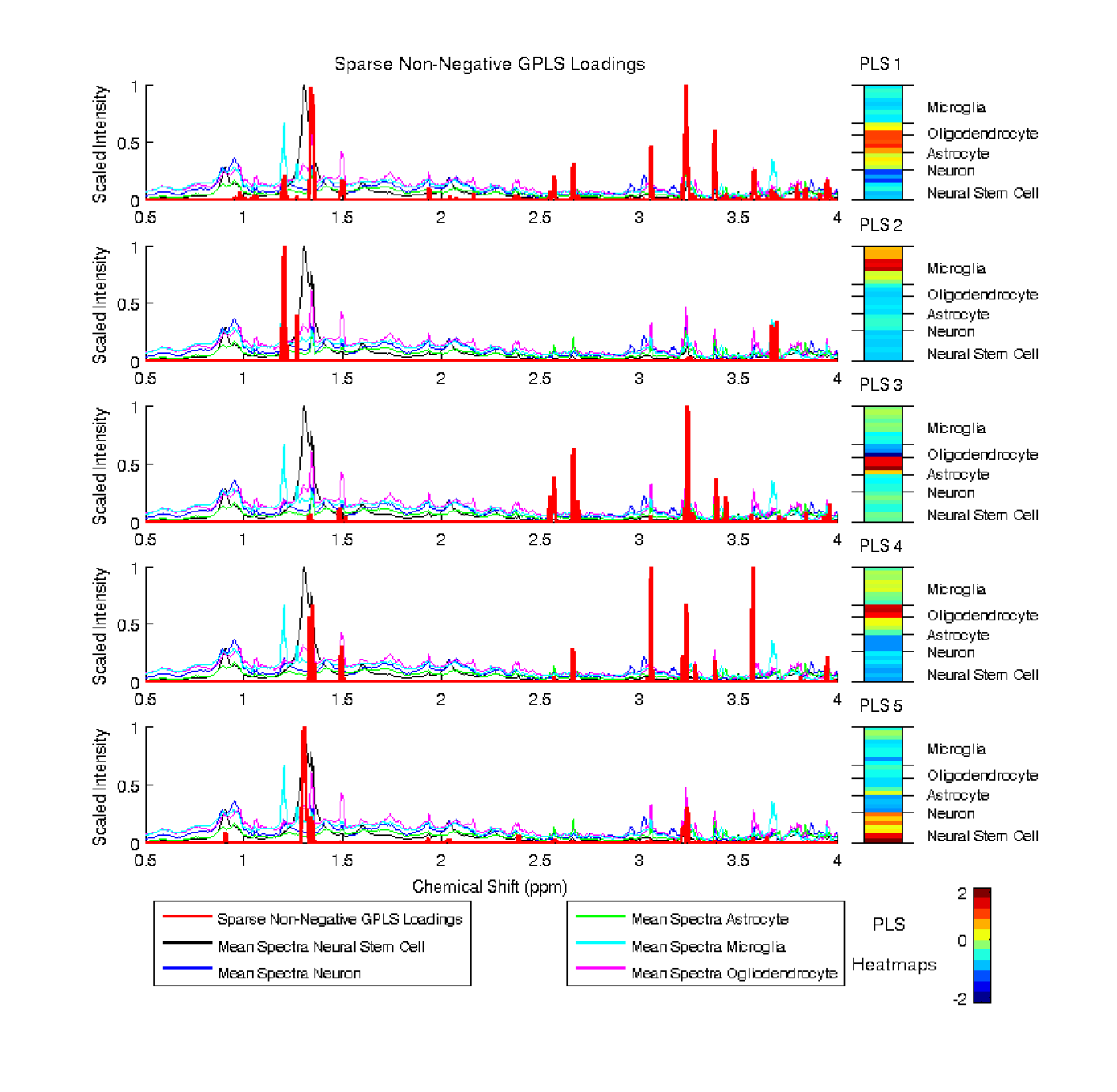
Figure 1: Sparse Non-negative Generalized PLS loadings and sample PLS heatmaps for the neural cell NMR data. The loadings are superimposed on the mean scaled spectral intensities for each class of neural cells.

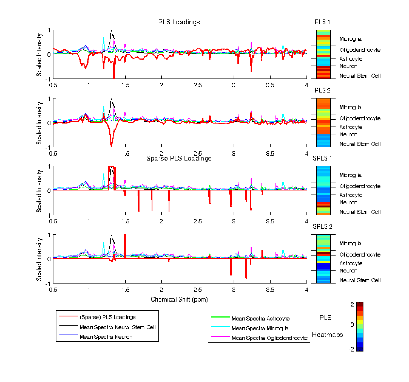
Figure 2: The first two PLS and Sparse PLS (Chun and Keleş, 2010) loadings and sample PLS heatmaps for the neural cell NMR data. The loadings are superimposed on the mean scaled spectral intensities for each class of neural cells.

In Table  3, we give the training and leave-one out cross-validation misclassification errors for our methods and competing methods on the neural cell NMR data. Notice that our Sparse GPLS method yields the best error rates followed by the Sparse PLS (Chun and Keleş, 2010) and our GPLS methods. Additionally, our Sparse GPLS methods are significantly faster than competing approaches. In Table  4, the time in seconds to compute the entire solution path (51 values of $\lambda$) is reported. Timing comparisons were done on a Intel Xeon X5680 3.33Ghz processor using single-threaded scripts.

In addition to faster computation and better classification rates, our method’s flexibility leads to easily interpretable results. We present the Sparse GPLS loadings superimposed on the scaled spectra from each neural cell type and sample heatmaps in Figure 1. For comparison, we give the first two PLS loadings in Figure 2 for PLS and Sparse PLS (Chun and Keleş, 2010). The PLS loadings are noisy, and the sample PLS components for PLS and Sparse PLS are difficult to interpret as the loadings are both positive and negative. By constraining the PLS loadings to be non-negative, the chemical shifts the metabolites indicative of each neural cell type are readily apparent with the Sparse Non-negative GPLS loadings. Additionally as shown in the sample PLS heatmaps, the neural cell types are well differentiated. For example, chemical resonances at 1.30ppms ad 3.23ppms characterize Glia (Astrocytes and Ogliodendrocytes) and Neurons (PLS 1), resonances at 1.19ppms and 3.66ppms characterize Microglia (PLS 2), resonances at 3.23ppms 2.65ppms characterize Astrocytes (PLS 3), resonances at 1.30ppms, 3.02ppms, and 3.55ppms characterize Ogliodendrocytes (PLS 4), and resonances at 1.28ppms and 3.23ppms characterize Neural stem cells. Note that some of these metabolites were identified by some of the same authors using PCA methods in Manganas et al. (2007); Allen and Maletić-Savatić (2011). Using our flexible PLS approach for supervised dimension reduction, however, gives a much clear metabolic signature of each neural cell type. Overall, this case study on NMR spectroscopy data has revealed the many strengths of our method as well as identified possible metabolite biomarkers for further biological investigation.

6 Discussion

We have presented a framework for regularizing partial least squares with convex and order one penalties. Additionally, we have shown how this approach can be extend for structured data via Generalized PLS and RPLS and extended to incorporate non-negative PLS or RPLS loadings. Our approaches directly solve penalized relaxations of the SIMPLS optimization criterion. These in turn, have many advantages including computational efficiency, flexible modeling, easy interpretation and visualization, better feature selection, and improved predictive accuracy as demonstrated in our simulations and case study on NMR spectroscopy.

There are many future areas of research related to our methodology. While we have briefly discussed the use of our methods for general regression or classification procedures, specific investigation of the RPLS factors as predictors in the generalized linear model framework (Marx, 1996; Chung and Keles, 2010), the survival analysis framework (Nguyen and Rocke, 2002a), and others are needed. Additionally, following the close connection of PLS for classification with the classes coded as dummy variables to Fisher’s discriminant analysis (Barker and Rayens, 2003), our RPLS approach may give an alternative strategy for regularized linear discriminant analysis. Further development of our novel extensions for GPLS and Non-negative PLS is also needed. Finally, Nadler and Coifman (2005) and Chun and Keleş (2010) have shown asymptotic inconsistency of PLS regression methods when the number of variables is permitted to grow faster than the sample size. For related PCA methods, a few have shown consistency of Sparse PCA in these settings (Johnstone and Lu, 2009; Amini and Wainwright, 2009). Proving consistent recovery of the RPLS loadings and the corresponding regression or classification coefficients is an open area of future research.

Finally, we have demonstrated the utility of our methods through a case study on NMR spectroscopy data, but there are many other potential applications of our technology. These include chemometrics, proteomics, metabolomics, high-throughput genomics, imaging, hyperspectral imaging and neuroimaging. Overall, we have presented a flexible and powerful tool for supervised dimension reduction of high-dimensional data with many advantages and potential areas of future research and application. An R package and a Matlab toolbox named RPLS that implements our methods will be made publicly available.

7 Acknowledgments

The authors would like to thank Frederick Campbell and Han Yu for assistance with the software development for this paper. C. Peterson acknowledges support from the Keck Center of the Gulf Coast Consortia, on the NLM Training Program in Biomedical Informatics, National Library of Medicine (NLM) T15LM007093; M. Vannucci and M. Maletić-Savatić are partially supported by the Collaborative Research Fund from the Virgina and L. E. Simmons Family Foundation.

Appendix A Proofs

Proof of Proposition 1.

The proof of this result follows from an argument in Allen et al. (2011), but we outline this here for completion. The updates for $\operatorname{\mathbf{u}}$ are straightforward. We show that the sub-gradient equations of the penalized regression problem, $\frac{1}{2}||\operatorname{\mathbf{M}}\operatorname{\mathbf{u}}-\operatorname{\mathbf{v}}||+\lambda P(\operatorname{\mathbf{v}})$, for $\operatorname{\mathbf{v}}^{*}$ as defined in the stated result are equivalent to the KKT conditions of (1). The sub-gradient equation of the latter is, $\operatorname{\mathbf{M}}\operatorname{\mathbf{u}}-\lambda\nabla P(\operatorname{\mathbf{v}}^{*})-2\gamma^{*}\operatorname{\mathbf{v}}^{*}=0$, where $\nabla P()$ is the sub-gradient of $P()$ and $\gamma^{*}$ is the Lagrange multiplier for the inequality constraint with complementary slackness condition, $\gamma^{*}((\operatorname{\mathbf{v}}^{*})^{T}\operatorname{\mathbf{v}}^{*}-1)=0$. The sub-gradient of the penalized regression problem is $\operatorname{\mathbf{M}}\operatorname{\mathbf{u}}-\hat{\operatorname{\mathbf{v}}}-\lambda\nabla P(\hat{\operatorname{\mathbf{v}}})=0$. Now, since $P()$ is order one, we this sub-gradient is equivalent to $\operatorname{\mathbf{M}}\operatorname{\mathbf{u}}-\frac{1}{c}\tilde{\operatorname{\mathbf{v}}}-\lambda\nabla P(\tilde{\operatorname{\mathbf{v}}})$ for any $c>0$ and for $\tilde{\operatorname{\mathbf{v}}}=c\hat{\operatorname{\mathbf{v}}}$. Then, taking $c=1/||\hat{\operatorname{\mathbf{v}}}||_{2}=1/2\gamma^{*}$ for any $\hat{\operatorname{\mathbf{v}}}\neq 0$, we see that both the complimentary slackness condition is satisfied and the sub-gradients are equivalent. It is easy to verify that the pair $(0,0)$ also satisfy the KKT conditions of (1). ∎

Proof of Corollary 1.

The proof of this fact follows in a straightforward manner from that of Proposition 1 as the only feasible solution for $\operatorname{\mathbf{u}}$ is $\operatorname{\mathbf{u}}^{*}=1$. We are then left with a concave optimization problem, $\operatorname*{\mathrm{maximize}}_{\operatorname{\mathbf{v}}}\ \operatorname{\mathbf{v}}^{T}\operatorname{\mathbf{M}}-\lambda P(\operatorname{\mathbf{v}})\ \textrm{subject to}\ \operatorname{\mathbf{v}}^{T}\operatorname{\mathbf{v}}\leq 1$. From the proof of Proposition 1, we have that this optimization problem is equivalent to the desired result. Since we are left with a concave problem, the global optimum is achieved. ∎

Proof of Proposition 2.

First, define $\tilde{\operatorname{\mathbf{Q}}}$ to be a matrix square root of $\operatorname{\mathbf{Q}}$ as in Allen et al. (2011). In this paper, they showed that Generalized PCA was equivalent to PCA on the matrix $\tilde{\operatorname{\mathbf{X}}}=\operatorname{\mathbf{X}}\tilde{\operatorname{\mathbf{Q}}}$ for projected factors $\operatorname{\mathbf{V}}=\tilde{\operatorname{\mathbf{Q}}}^{\dagger}\tilde{\operatorname{\mathbf{V}}}$. In other words, if $\tilde{\operatorname{\mathbf{X}}}=\tilde{\operatorname{\mathbf{U}}}\tilde{\operatorname{\mathbf{D}}}\tilde{\operatorname{\mathbf{V}}}$ is the singular value decomposition, then the GPCA solution, $\operatorname{\mathbf{V}}$ can be defined accordingly. Here, we will prove that the multi-factor RPLS problem for $\tilde{\operatorname{\mathbf{X}}}$ and $\tilde{\operatorname{\mathbf{v}}}_{k}$ is equivalent to the stated Generalized RPLS problem (2) for $\lambda=0$. The constraint regions are trivially equivalent so we must show that $\tilde{\operatorname{\mathbf{v}}}_{k}^{T}\tilde{\operatorname{\mathbf{P}}}_{k-1}\tilde{\operatorname{\mathbf{M}}}=\operatorname{\mathbf{v}}^{T}\operatorname{\mathbf{Q}}\operatorname{\mathbf{P}}_{k-1}\operatorname{\mathbf{Q}}\operatorname{\mathbf{M}}$. The PLS factors, $\tilde{\operatorname{\mathbf{z}}}_{k}=\tilde{\operatorname{\mathbf{X}}}\tilde{\operatorname{\mathbf{v}}}_{k}=\operatorname{\mathbf{X}}\operatorname{\mathbf{Q}}\operatorname{\mathbf{v}}_{k}=\operatorname{\mathbf{z}}_{k}$, are equivalent. Ignoring the normalizing term in the denominator, the columns of the projection weighting matrix are $\tilde{\operatorname{\mathbf{R}}}_{k}=\tilde{\operatorname{\mathbf{X}}}^{T}\tilde{\operatorname{\mathbf{z}}}_{k}=\tilde{\operatorname{\mathbf{Q}}}^{T}\operatorname{\mathbf{X}}\operatorname{\mathbf{z}}_{k}=\tilde{\operatorname{\mathbf{Q}}}^{T}\operatorname{\mathbf{R}}_{k}$. Thus, the $ij^{th}$ element of $\tilde{\operatorname{\mathbf{R}}}^{T}\tilde{\operatorname{\mathbf{R}}}=\operatorname{\mathbf{z}}_{i}^{T}\operatorname{\mathbf{X}}\tilde{\operatorname{\mathbf{Q}}}\tilde{\operatorname{\mathbf{Q}}}^{T}\operatorname{\mathbf{X}}^{T}\operatorname{\mathbf{z}}_{j}=\operatorname{\mathbf{R}}_{i}^{T}\operatorname{\mathbf{Q}}\operatorname{\mathbf{R}}_{j}$ as stated. Putting these together, we have $\tilde{\operatorname{\mathbf{v}}}_{k}^{T}\tilde{\operatorname{\mathbf{P}}}_{k-1}\tilde{\operatorname{\mathbf{M}}}=\operatorname{\mathbf{v}}_{k}^{T}\tilde{\operatorname{\mathbf{Q}}}(\mathbf{I}-\tilde{\operatorname{\mathbf{R}}}_{k-1}(\operatorname{\mathbf{R}}_{k-1}^{T}\operatorname{\mathbf{Q}}\operatorname{\mathbf{R}}_{k-1})^{-1}\tilde{\operatorname{\mathbf{R}}}_{k-1}^{T})\tilde{\operatorname{\mathbf{Q}}}^{T}\operatorname{\mathbf{X}}^{T}\operatorname{\mathbf{Y}}$ which simplifies to the desired result.

Following this, the proof of the first part is a straightforward extension of Theorem 1 and Proposition 1 in Allen et al. (2011). The proof for the second part follows from combining the arguments in Proposition 1 and those in the proof of Theorem 2 in Allen et al. (2011). ∎

References

- Allen and Maletić-Savatić (2011) Allen, G. and M. Maletić-Savatić (2011). Sparse non-negative generalized pca with applications to metabolomics. Bioinformatics 27(21), 3029–3035.
- Allen et al. (2011) Allen, G. I., L. Grosenick, and J. Taylor (2011). A generalized least squares matrix decomposition. Rice University Technical Report No. TR2011-03.
- Amini and Wainwright (2009) Amini, A. and M. Wainwright (2009). High-dimensional analysis of semidefinite relaxations for sparse principal components. The Annals of Statistics 37(5B), 2877–2921.
- Bair et al. (2006) Bair, E., T. Hastie, D. Paul, and R. Tibshirani (2006). Prediction by supervised principal components. Journal of the American Statistical Association 101(473), 119–137.
- Barker and Rayens (2003) Barker, M. and W. Rayens (2003). Partial least squares for discrimination. Journal of chemometrics 17(3), 166–173.
- Boulesteix and Strimmer (2007) Boulesteix, A. and K. Strimmer (2007). Partial least squares: a versatile tool for the analysis of high-dimensional genomic data. Briefings in Bioinformatics 8(1), 32.
- Chun and Keleş (2010) Chun, H. and S. Keleş (2010). Sparse partial least squares regression for simultaneous dimension reduction and variable selection. Journal of the Royal Statistical Society: Series B (Statistical Methodology) 72(1), 3–25.
- Chung et al. (2012) Chung, D., H. Chun, and S. Keles (2012). spls: Sparse Partial Least Squares (SPLS) Regression and Classification. R package, version 2.1-1.
- Chung and Keles (2010) Chung, D. and S. Keles (2010). Sparse Partial Least Squares Classification for High Dimensional Data. Statistical applications in genetics and molecular biology 9(1).
- De Graaf (2007) De Graaf, R. (2007). In vivo NMR spectroscopy: principles and techniques. Wiley-Interscience.
- de Jong (1993) de Jong, S. (1993). SIMPLS: an alternative approach to partial least squares regression. Chemometrics and Intelligent Laboratory Systems 18(3), 251–263.
- Dunn et al. (2005) Dunn, W., N. Bailey, and H. Johnson (2005). Measuring the metabolome: current analytical technologies. Analyst 130(5), 606–625.
- Friedman et al. (2010) Friedman, J., T. Hastie, and R. Tibshirani (2010). Regularization paths for generalized linear models via coordinate descent. Journal of statistical software 33(1), 1.
- Goodacre et al. (2004) Goodacre, R., S. Vaidyanathan, W. Dunn, G. Harrigan, and D. Kell (2004). Metabolomics by numbers: acquiring and understanding global metabolite data. TRENDS in Biotechnology 22(5), 245–252.
- Goutis and Fearn (1996) Goutis, C. and T. Fearn (1996). Partial Least Squares Regression on Smooth Factors. Journal of the American Statistical Association 91(434).
- Horn and Johnson (1985) Horn, R. A. and C. R. Johnson (1985). Matrix Analysis. Cambridge University Press.
- Hoyer (2004) Hoyer, P. (2004). Non-negative matrix factorization with sparseness constraints. The Journal of Machine Learning Research 5, 1457–1469.
- Huang et al. (2004) Huang, X., W. Pan, S. Park, X. Han, L. Miller, and J. Hall (2004). Modeling the relationship between LVAD support time and gene expression changes in the human heart by penalized partial least squares. Bioinformatics, 4991.
- Johnstone and Lu (2009) Johnstone, I. and A. Lu (2009). On consistency and sparsity for principal components analysis in high dimensions. Journal of the American Statistical Association 104(486), 682–693.
- Jung and Marron (2009) Jung, S. and J. Marron (2009). Pca consistency in high dimension, low sample size context. The Annals of Statistics 37(6B), 4104–4130.
- Krämer (2007) Krämer, N. (2007). An overview on the shrinkage properties of partial least squares regression. Computational Statistics 22(2), 249–273.
- Krämer and Sugiyama (2011) Krämer, N. and M. Sugiyama (2011). The degrees of freedom of partial least squares regression. Journal of the American Statistical Association 106(494), 697–705.
- Lee and Seung (1999) Lee, D. and H. Seung (1999). Learning the parts of objects by non-negative matrix factorization. Nature 401(6755), 788–791.
- Lee et al. (2010) Lee, M., H. Shen, J. Huang, and J. Marron (2010). Biclustering via Sparse Singular Value Decomposition. Biometrics 66(4), 1087–1095.
- Manganas et al. (2007) Manganas, L., X. Zhang, Y. Li, R. Hazel, S. Smith, M. Wagshul, F. Henn, H. Benveniste, P. Djurić, G. Enikolopov, et al. (2007). Magnetic resonance spectroscopy identifies neural progenitor cells in the live human brain. Science 318(5852), 980.
- Marx (1996) Marx, B. (1996). Iteratively reweighted partial least squares estimation for generalized linear regression. Technometrics, 374–381.
- Nadler and Coifman (2005) Nadler, B. and R. Coifman (2005). The prediction error in cls and pls: the importance of feature selection prior to multivariate calibration. Journal of chemometrics 19(2), 107–118.
- Nguyen and Rocke (2002a) Nguyen, D. and D. Rocke (2002a). Partial least squares proportional hazard regression for application to dna microarray survival data. Bioinformatics 18(12), 1625–1632.
- Nguyen and Rocke (2002b) Nguyen, D. and D. Rocke (2002b). Tumor classification by partial least squares using microarray gene expression data. Bioinformatics 18(1), 39–50.
- Nicholson and Lindon (2008) Nicholson, J. and J. Lindon (2008). Systems biology: metabonomics. Nature 455(7216), 1054–1056.
- Owen and Perry (2009) Owen, A. and P. Perry (2009). Bi-cross-validation of the SVD and the nonnegative matrix factorization. Annals 3(2), 564–594.
- Reiss and Ogden (2007) Reiss, P. and R. Ogden (2007). Functional principal component regression and functional partial least squares. Journal of the American Statistical Association 102(479), 984–996.
- Rossouw et al. (2008) Rossouw, D., C. Robert-Granié, and P. Besse (2008). A sparse pls for variable selection when integrating omics data. Genetics and Molecular Biology 7(1), 35.
- Shen and Huang (2008) Shen, H. and J. Huang (2008). Sparse principal component analysis via regularized low rank matrix approximation. Journal of multivariate analysis 99(6), 1015–1034.
- Tibshirani (1996) Tibshirani, R. (1996). Regression shrinkage and selection via the lasso. Journal of the Royal Statistical Society. Series B (Methodological), 267–288.
- Tibshirani et al. (2005) Tibshirani, R., M. Saunders, S. Rosset, J. Zhu, and K. Knight (2005). Sparsity and smoothness via the fused lasso. Journal of the Royal Statistical Society: Series B (Statistical Methodology) 67(1), 91–108.
- Witten et al. (2009) Witten, D., R. Tibshirani, and T. Hastie (2009). A penalized matrix decomposition, with applications to sparse principal components and canonical correlation analysis. Biostatistics 10(3), 515.
- Wold (1966) Wold, H. (1966). Estimation of principal components and related models by iterative least squares. Multivariate analysis 1, 391–420.
- Yuan and Lin (2006) Yuan, M. and Y. Lin (2006). Model selection and estimation in regression with grouped variables. Journal of the Royal Statistical Society: Series B (Statistical Methodology) 68(1), 49–67.
- Zou et al. (2006) Zou, H., T. Hastie, and R. Tibshirani (2006). Sparse principal component analysis. Journal of computational and graphical statistics 15(2), 265–286.