Examination of the mass-dependent Li depletion hypothesis by the Li abundances of the very metal-poor double-lined spectroscopic binary G 166–45

Abstract

The Li abundances of the two components of the very metal-poor ([Fe/H]$=-2.5$) double-lined spectroscopic binary G 166–45 (BD+26^∘2606) are determined separately based on high resolution spectra obtained with the Subaru Telescope High Dispersion Spectrograph and its image slicer. From the photometric colors and the mass ratio the effective temperatures of the primary and secondary components are estimated to be 6350$\pm 100$ K and 5830$\pm 170$ K, respectively. The Li abundance of the primary ($A$(Li)$=2.23$) agrees well with the Spite plateau value, while that of the secondary is slightly lower ($A$(Li)$=2.11$). Such a discrepancy of the Li abundances between the two components is previously found in the extremely metal-poor, double-lined spectroscopic binary CS 22876–032, however, the discrepancy in G 166–45 is much smaller. The results agree with the trends found for Li abundance as a function of effective temperature (and of stellar mass) of main-sequence stars with $-3.0<$[Fe/H]$<-2.0$, suggesting that the depletion of Li at $T_{\rm eff}$$\sim 5800$ K is not particularly large in this metallicity range. The significant Li depletion found in CS 22876–032B is a phenomenon only found in the lowest metallicity range ([Fe/H]$<-3$).

1 Introduction

Lithium is an important element as a diagnostic of the structure and evolution of low-mass stars. Since Li is easily destroyed by nuclear fusion in the hot interiors of stars where the temperature is above 2.5 $\times 10^{6}$ K, stellar internal processes can be examined from observed Li abundances at stellar surface. Li depletion processes also play an important role in reconciling the serious discrepancy between the observed constant Li abundance, the so-called Spite plateau, of metal-poor turnoff stars ($A$(Li) = $\log$(Li/H)+12 $\sim$ 2.2: e.g., Spite & Spite (1982); Asplund et al. (2006)) and the primordial Li abundance predicted from standard Big Bang nucleosynthesis (SBBN) models adopting the baryon density determined from observations of the cosmic microwave background (CMB) by the WMAP satellite ($A$(Li) $=2.72$: e.g. Cyburt et al. 2008). The discrepancy seems to be larger at lower metallicity (Bonifacio et al. 2007; Aoki et al. 2009; Sbordone et al. 2010). If the stellar intrinsic Li depletion is in operation in the atmospheres of metal-poor turnoff stars, the observed Li abundance is lower than the initial value, which may have been closer to the CMB and SBBN prediction.

Although no Li depletion is inferred for metal-poor stars on the main-sequence-turn-off by standard stellar evolution theories because of their shallow convection zones, evolutionary models that include effects of atomic diffusion (e.g., Richard et al. 2002a, b) predict significant decline of surface Li abundances for metal-poor dwarfs. Richard et al. (2005) additionally introduced parametrized effects of turbulent mixing to their evolution model for [Fe/H] $=-2.31$ , though the understanding of the physics of the turbulent mixing is still insufficient. Korn et al. (2006) and Korn et al. (2007) investigated effects of these processes for the globular cluster NGC 6397 by examining small variations of Mg, Ca, Ti and Fe abundances in main-sequence turnoff, subgiant and giant stars. They suggested diffusion process during main-sequence phase and attributed the slightly lower Li abundances in turn-off stars than in subgiants to these effects.

The most convincing evidence of stellar Li depletion in metal-poor dwarfs found so far is the large difference between Li abundances of the primary and secondary dwarf stars in the extremely metal-poor ([Fe/H]$=-3.6$) double-lined spectroscopic binary CS 22876–032, which is about 0.4 dex (González Hernández et al. 2008). Since the two stars should have shared the same chemical compositions at their birth, it is reasonable to presume that depletion processes have made the Li abundance difference during the stellar evolution. Such depletion is not expected for a star with the effective temperature of the secondary ($T_{\rm eff}$$=5900$ K) from previous studies of less metal-poor stars. Given that the mass of the secondary star is about 0.9 times that of the primary, Li depletion may operate mass-dependently, which is consistent with the predictions of Richard et al. (2005), as discussed by Meléndez et al. (2010).

The best approach to examine the hypothesis of the mass-dependent lithium depletion is accurate determinations of Li abundances for several metal-poor binary stars. Although Meléndez et al. (2010) suggested a correlation between Li abundance and stellar mass for metal-poor single stars, investigation of single stars which have different ages and distances would suffer from uncertainties in mass estimates.

In this Letter, we report our chemical abundance analysis, in particular the Li abundances, of the two components of the very metal-poor, double-lined spectroscopic binary G 166–45. This object is selected from the sample of Goldberg et al. (2002) who investigated the orbital parameters of 34 binary stars found by the Carney-Latham proper motion sample (Carney et al. 1994). The chemical abundances of individual components of this object have not yet been investigated. We discuss in particular the implication of the small difference of the Li abundance between the two components found from the present analysis of high resolution spectra.

2 Observations and measurements

A high-resolution spectrum of G 166–45 was obtained with the Subaru Telescope High Dispersion Spectrograph (HDS; Noguchi et al. 2002) on July 22, 2011. We applied the image slicer recently installed in the spectrograph, which provides the resolving power of $R=110,000$ with high efficiency (Tajitsu et al. 2012). The wavelength range from 5100 to 7800 Å is covered by the standard setup of StdRa. The exposure time is 60 minutes, resulting in the S/N ratio (per 0.9  km s^-1 pixel) of 350 at 6700 Å.

According to the orbital parameters of the binary determined by Goldberg et al. (2002), the velocity difference between the two components of this object is expected to be 15–20  km s^-1 at this epoch. Indeed, the separation of the absorption features in our spectrum is 18.5  km s^-1 (see below), agreeing well with the above estimate.

Standard data reduction was carried out with the IRAF echelle package. Spectra are extracted from individual sliced images and combined for the slice numbers 2–5 in the definition of Tajitsu et al. (2012) to obtain the best quality spectrum.

Equivalent widths ($W$’s) for isolated absorption lines were measured by fitting Gaussian profiles for each component of the binary. The equivalent widths are used in the following chemical abundance analysis by dividing the fraction of the contribution of each component to the continuum flux estimated from colors and mass ratio of the two components (§ 3).

3 Analysis and results

3.1 Atmospheric Parameters

In order to determine the atmospheric parameters of the two components of the binary system and their contributions to the continuum flux, we adopt the mass ratio of the two components ($q=m_{2}/m_{1}=0.89\pm 0.04$), where $m_{1}$ and $m_{2}$ are the primary and secondary masses, respectively, determined by Goldberg et al. (2002), and calculate the colors ($B-V$, $V-R$, and $V-I$) as a function of the primary mass using the $Y^{2}$ isochrone (Demarque et al. 2004) for the age of 12 Gyr. The metallicity is assumed to be [Fe/H]$=-2.5$, which is consistent with the results obtained from the following analysis.

The upper panel of Figure 1 shows the three colors calculated using the isochrone. Solid and dotted lines indicate the cases of $q=0.89$ and those with 0.04 higher or lower, respectively. Very accurate colors of G 166–45 are available, because this object is a Landolt’s photometric standard star. The colors measured by their recent work (Landolt & Uomoto 2007) with a reddening correction are shown by the horizontal lines in the figure. The reddening correction ($E(B-V)=0.02$) is estimated from the interstellar Na I D₂ line detected in our spectrum (the equivalent width of 80 mÅ).

Comparisons of these colors with the calculations provide constraints on the primary mass of this binary system (as well as the secondary mass). The primary mass estimated from the three colors is $0.757\pm 0.007$M_⊙, in which the error corresponds to the differences of the results from the three colors. Even if the photometry error (0.015 mag) for G 166–45 estimated by Landolt & Uomoto (2007) (see the erratum of the paper) and the uncertainty of the mass ratio are included, the error size of the primary mass does not change significantly. The other solution that satisfies the colors and the mass ratio is the case that the primary is a subgiant ($m_{1}\sim 0.82~{}$M_⊙) and the secondary is a main-sequence star with similar temperatures (see Fig. 1). This solution is, however, excluded because the luminosity difference of the two components can not be so large, given the strengths of the absorption features of the two components.

The lower panel of Figure 1 shows the effective temperatures of the primary and secondary, as a function of the primary mass (assuming the mass ratio), adopted from the $Y^{2}$ isochrone. The effective temperature of the primary is well determined to be 6350$\pm 100$ K. The error reflects the uncertainty of the mass determination from different color indices and photometric errors, but does not include the uncertainty of the temperature scale (depending on model atmospheres).

By contrast, the uncertainty of the effective temperature of the secondary is relatively large (170 K) due to the uncertainty of the mass ratio. We adopt 5830 K for the secondary as the best estimate in the following analysis, but also conduct the analyses for $T_{\rm eff}$ = 5650 and 6000 K to estimate the errors due to the uncertainty of the mass ratio. The surface gravities of the primary and the secondary are estimated from the isochrone to be $\log g=4.4$ and 4.6, respectively.

The fraction of the contributions of each component to the continuum flux in the $R$-band ($f$: $f_{\rm A}$ and $f_{\rm B}$ for the primary and secondary, respectively), in which the Li I resonance line exists, is also estimated from the isochrone for the three choices of the secondary’s effective temperature.

The adopted parameter sets ($T_{\rm eff}$, $\log g$, and $f_{\rm B}$) are (5830 K, 4.6, 0.27), (5650 K, 4.6, 0.21) and (6000 K, 4.6, 0.34) for the secondary, while $T_{\rm eff}$ = 6350 K, $\log g$ = 4.4, and $f_{\rm A}=1-f_{\rm B}$ are adopted for the primary (Table 1).

For comparison purposes, we applied the above procedure to the double-lined spectroscopic binary CS 22876–032 adopting the mass ratio of 0.91 (González Hernández et al. 2008) and colors given by Norris et al. (2000). The results agree well with those determined by González Hernández et al. (2008), i.e., 6500 K and 5900 K for the primary and secondary, respectively, with uncertainties of about 100 K.

3.2 Chemical abundances

Chemical compositions of the two components of this binary system are determined separately based on the standard LTE analysis of the equivalent widths obtained by dividing the measured equivalent widths from the spectrum by the $f$. The ATLAS NEWODF model atmosphere grid (Castelli & Kurucz 2003) assuming $\alpha$ elements excesses is used in the analysis.

The micro-turbulent velocity ($v_{\rm micro}$) is determined by demanding no dependence of the abundance results for individual Fe I lines on their strengths (equivalent widths). The derived $v_{\rm micro}$ is 1.5  km s^-1 for the primary and 1.0  km s^-1 for the secondary.

The results of the abundance analyses are given in Table 1 for eight elements (along with the Li abundance determined separately) for the standard case of the stellar parameters. We also give the results of Fe abundances for the other parameter sets in the table. The errors given in Table 1 include random errors and those due to uncertainties of atmospheric parameters. We estimate the random errors in the measurements to be $\sigma/N$, where $\sigma$ is the standard deviation of derived abundances from individual lines and $N$ is the number of lines used. When only a few lines are available, the $\sigma$ of Fe I is adopted in the estimates. The errors due to the uncertainty of the atmospheric parameters ($\delta$$T_{\rm eff}$$=100$ K, $\delta$$\log g$$=0.3$, and $\delta$$v_{\rm micro}$$=0.2$  km s^-1) are also estimated and added in quadrature to the random errors. The errors for the secondary could be slightly larger if the the uncertainty of effective temperature due to the uncertainty of the mass ratio ($\sim 170$ K) is included.

The Fe abundances derived from individual Fe I lines show no statistically significant dependence on their lower excitation potentials for the three choices of the stellar parameters. The Fe abundance derived from Fe II lines is slightly higher than that from Fe I lines, suggesting the $\log g$ values adopted in the analysis are systematically too high (by 0.1–0.3 dex), or the Fe I lines suffer from non-LTE effects (e.g., Asplund 2005). We note that the Li line analysis reported in the following subsection is not sensitive to the changes of the adopted $\log g$ and $v_{\rm micro}$.

The chemical compositions of the two components agree very well with each other. The changes of the Fe abundance from Fe I lines by changing the choice of stellar parameter set are only 0.05 dex for the primary. The change for the secondary is even smaller, because the effect of the change of $T_{\rm eff}$ on the derived Fe abundance is partially compensated by the change of the contribution of the secondary to the continuum flux (adopting a higher $T_{\rm eff}$ results in a higher Fe abundance in general, while a larger $f_{\rm B}$ results in smaller equivalent widths and a lower abundance).

3.3 Li abundances

The Li abundances of the two components of G 166–45 are determined by fitting synthetic spectra to the observed one. The synthetic spectra are calculated using the same model atmospheres used in the above subsection for both components, and are combined taking their $f$’s into account and the velocity shift between them (18.5  km s^-1). Comparisons of the synthetic spectra with the observed one are depicted in Figure 2, where the doppler correction is made for the primary. In the fitting process, the $\chi^{2}$ minimum is searched for each component: the wavelength ranges 6707.6–6708.0 Å and 6708.0–6708.4 Å are used to determine the Li abundances of the primary and secondary, respectively. The $2\sigma$ error in the fitting is 0.02 and 0.03 dex for the primary and secondary, respectively.

The results for the three choices of mass ratios are given in Table 1. Interestingly, the Li abundance of the secondary is insensitive to the choice of the mass ratio for the same reason for the behavior of the Fe abundance mentioned above.

The derived Li abundance of the secondary is 0.05–0.15 dex lower than that of the primary. In the following discussion on the Li abundance difference between the two components, we take the fitting errors (0.02–0.03 dex) and the errors due to the uncertainty of the mass ratio (0.02–0.05 dex) into consideration. We note that this does not include the error due to the uncertainty of $T_{\rm eff}$ scales, which is as large as 0.1 dex in $A$(Li), but is a systematic error affecting the results for both components.

4 Discussion and concluding remarks

The Li abundance of the primary derived by the above analysis ($A$(Li)$=2.23\pm 0.05$) well agrees with the Spite plateau value, while that of the secondary is slightly lower. Figure 3 (top panel) depicts the Li abundances of main-sequence ($\log g$$>4.0$: filled symbols) and subgiant ($\log g$$<4.0$: open symbols) stars as a function of [Fe/H]. The data other than G 166–45 are adopted from González Hernández et al. (2008) for CS 22876–032 and Meléndez et al. (2010) for other stars determined by LTE analyses. The possible Li depletion in the main-sequence phase can be inspected from filled symbols shown here. While large scatter of Li abundances is found in [Fe/H]$>-2$, which is due to the lower abundances in stars with lower $T_{\rm eff}$ (see below), there is no distinctive scatter in $-3<$[Fe/H]$<-2$ in this sample. This is not changed even if subgiants ($\log g$$<4$) are included. Meléndez et al. (2010) suggested the existence of two plateaus with slightly higher and lower Li abundances in [Fe/H]$>-2.5$ and $<-2.5$, respectively. The Li abundance of G 166–45A is apparently in agreement with the lower plateau. This result is, however, not definitive, given a possible systematic offset in Li abundance determinations (as large as 0.1 dex) mostly due to $T_{\rm eff}$ scales used. Among the stars in this metallicity range, the Li abundance of G 166–45B is relatively low.

Some scatter of Li abundances is also found in [Fe/H]$<-3$, though that is smaller than that in [Fe/H]$>-2$. The discrepancy of the two components of CS 22876–032 is consistent with the size of the scatter.

The middle panel of Figure 3 shows the Li abundances as a function of $T_{\rm eff}$. A clear dependence of Li abundances on $T_{\rm eff}$ is found in $T_{\rm eff}$$<6000$ K. It should be noted that all stars in this temperature range, except for CS 22876–032B and two subgiants, are objects with [Fe/H]$>-2$. The difference of Li abundances between objects with $T_{\rm eff}$$\sim 6350$ K and those with $\sim$5830 K is as large as 0.4 dex. The discrepancy of the Li abundances found between the two components of G 166–45 is much smaller than this value. This suggests that the depletion of Li in stars with $T_{\rm eff}$$\sim 5800$ K is much smaller at this metallicity ([Fe/H]$\sim-2.5$) than that in [Fe/H]$>-2$. This might be related to the shallower convection zone in stars with lower metallicity, however, other causes for Li depletion would be required as mentioned by Richard et al. (2005), who demonstrated that the temperature of the bottom of the convective zone is almost independent of metallicity. It should also be noted that subgiants ($\log g$$<4.0$) with $T_{\rm eff}$$<6000K$ have Li abundances as high as stars with $T_{\rm eff}$$>6000$ K, hence, the correlation between the Li abundance and $T_{\rm eff}$ discussed above is only found in main-sequence stars with high [Fe/H] ($>-2$). The exception is CS 22876–032B, which shows a Li abundance along with the correlation found for stars with [Fe/H]$>-2$. The reason for the Li depletion in this object is, however, likely different from the $T_{\rm eff}$-dependent depletion found for [Fe/H]$>-2$ (see below).

The bottom panel of Figure 3 shows Li abundances as a function of stellar mass. Li depletion in lower mass stars is discussed by Meléndez et al. (2010). Excluding the stars with [Fe/H]$>-2$ (indicated by triangles), which show a tight correlation between Li abundances and $T_{\rm eff}$, the dependence of the Li abundance on stellar mass is not very clear. Indeed, Meléndez et al. (2010) reported that the slopes of Li abundances as a function of stellar masses is significant at only 1$\sigma$ level in [Fe/H]$<-2.5$, which increases to the 3$\sigma$ level by including the binary CS 22876–032. However, if stars with lowest metallicity ([Fe/H]$<-3$) are selected, a correlation seems to appear again. In order to demonstrate this, stars in this metallicity range are indicated by over-plotting open circles (except for CS 22876–032) in the bottom panel of the figure.

On the other hand, no clear correlation is found between the Li abundances and stellar masses for objects with $-3<$[Fe/H]$<-2$ (squares without open circles). Our study of the Li abundance of G 166–45 B extends this trend to a mass below 0.7 M_⊙.

The dependence of Li abundances on stellar mass and metallicity is nonlinear. In [Fe/H]$>-2$, Li abundances are lower in main-sequence stars with lower $T_{\rm eff}$ (lower mass) in $T_{\rm eff}$$\lesssim 6000$ K ($M\lesssim 0.8$M_⊙). A similar dependence is also found in [Fe/H]$<-3$, possibly in stars with even higher $T_{\rm eff}$ ($\lesssim 6300$ K, which corresponds to $M\lesssim 0.8$M_⊙). On the other hand, such a dependence is not clearly seen in $-3<$[Fe/H]$<-2$. The double-lined spectroscopic binaries CS 22876–032 and G 166–45 most clearly represent these trends in [Fe/H]$<-3$ and $-3<$[Fe/H]$<-2$, respectively. Since the initial abundances of the two components of a binary system can be assumed to be the same, the discrepancy of the Li abundances found between the two components indicates a depletion of Li in the secondary. This suggests that the scatter of Li found in the lowest metallicity range is due to depletion of Li in some object, which is not clearly seen in $-3<$[Fe/H]$<-2$.

Figure 1: Upper panel: Colors ($V-I,B-V,V-R$) calculated from the isochrones assuming mass ratios of $q=0.89\pm 0.04$. The reddening corrected colors of G 166–45 are shown by horizontal lines. The vertical solid and dashed lines indicate the adopted primary mass and its possible range estimated from the three colors. Lower panel: effective temperatures of primary (thick solid line) and secondary (thin solid line and dotted lines) as a function of assumed primary mass adopting the above mass ratios.

Figure 2: Comparisons of synthetic spectra for the Li line with the observed one for the two components of G 166–45. Three different Li abundances ($\pm 0.05$ dex in $A$(Li)) for the results for the standard parameter set (see text) are assumed for each component in the calculations.

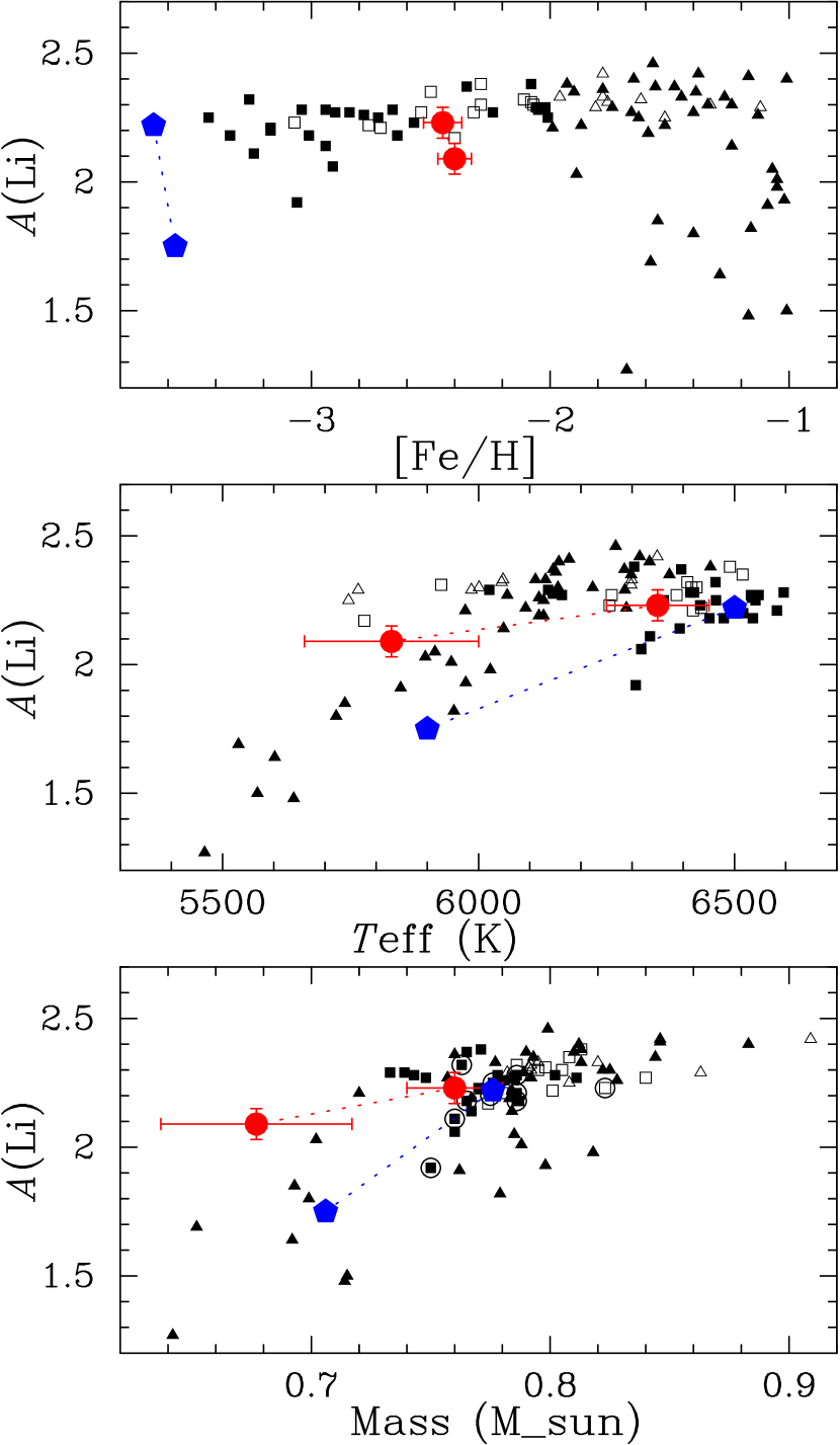
Figure 3: Li abundances as functions of [Fe/H], $T_{\rm eff}$ and stellar mass. Filled circles with error bars indicate G 166–45 A and B, while filled pentagons mean CS 22876–032A and B (González Hernández et al. 2008): the secondary stars have lower Li abundances. Filled squares and triangles are ’main-sequence’ ($\log g\geq 4.0$) stars with [Fe/H]$<-2$ and $>-2$, respectively, and open squares and triangles are ’subgiant’ ($\log g<4.0$) stars with [Fe/H]$<-2$ and $>-2$, respectively (Meléndez et al. 2010). In the bottom panel, objects with [Fe/H]$<-3$ are indicated by over-plotting large open circles.

Table 1: STELLAR PARAMETERS AND CHEMICAL ABUNDANCES

		G 166–45A				G 166–45B
$q=0.89$	$T_{\rm eff}$=6350 K, $f_{\rm A}=0.73$				$T_{\rm eff}$=5830 K, $f_{\rm B}=0.27$
Species	$\log\epsilon$	[X/Fe]([Fe/H])	$n$	error	$\log\epsilon$	[X/Fe]([Fe/H])	$n$	error
Fe I	5.05	$-2.45$	35	0.10	5.10	$-2.40$	39	0.11
Fe II	5.15	$-2.35$	3	0.14	5.30	$-2.20$	2	0.15
Na I	3.74	$-0.05$	2	0.09	3.76	$-0.08$	2	0.09
Mg I	5.44	$0.29$	3	0.09	5.31	$0.11$	3	0.12
Ca I	4.22	$0.34$	8	0.08	4.20	$0.26$	8	0.08
Ti II	3.00	$0.50$	3	0.13	3.01	$0.46$	3	0.13
Cr I	3.13	$-0.06$	3	0.10	3.14	$-0.10$	3	0.10
Ni I	3.90	$0.13$	1	0.13	4.17	$0.35$	2	0.13
Ba II	$-$0.47	$-0.20$	1	0.14	$\cdots$	$\cdots$	$\cdots$	$\cdots$
Li I	2.23	$\cdots$	1	0.02	2.11	$\cdots$	1	0.03
$q=0.93$	$T_{\rm eff}$=6350 K, $f_{\rm A}=0.66$				$T_{\rm eff}$=6000 K, $f_{\rm B}=0.34$
Fe I	5.11	$-2.39$	35	0.10	5.09	$-2.42$	39	0.11
Fe II	5.13	$-2.37$	3	0.14	5.19	$-2.31$	2	0.15
Li I	2.27	$\cdots$	1	0.02	2.12	$\cdots$	1	0.03
$q=0.85$	$T_{\rm eff}$=6350 K, $f_{\rm A}=0.79$				$T_{\rm eff}$=5670 K, $f_{\rm B}=0.21$
Fe I	5.00	$-2.50$	35	0.10	5.14	$-2.36$	39	0.11
Fe II	5.04	$-2.46$	3	0.14	5.43	$-2.07$	2	0.15
Li I	2.18	$\cdots$	1	0.02	2.13	$\cdots$	1	0.03

References

- Aoki et al. (2009) Aoki, W., Barklem, P. S., Beers, T. C., et al. 2009, ApJ, 698, 1803
- Asplund (2005) Asplund, M. 2005, ARA&A, 43, 481
- Asplund et al. (2006) Asplund, M., Lambert, D. L., Nissen, P. E., Primas, F., & Smith, V. V. 2006, ApJ, 644, 229
- Bonifacio et al. (2007) Bonifacio, P., Molaro, P., Sivarani, T., et al. 2007, A&A, 462, 851
- Carney et al. (1994) Carney, B. W., Latham, D. W., Laird, J. B., & Aguilar, L. A. 1994, AJ, 107, 2240
- Castelli & Kurucz (2003) Castelli, F., & Kurucz, R. L. 2003, Modelling of Stellar Atmospheres, 210, 20P
- Cyburt et al. (2008) Cyburt, R. H., Fields, B. D., & Olive, K. A. 2008, J. Cosmology Astropart. Phys, 11, 12
- Demarque et al. (2004) Demarque, P., Woo, J.-H., Kim, Y.-C., & Yi, S. K. 2004, ApJS, 155, 667
- Goldberg et al. (2002) Goldberg, D., Mazeh, T., Latham, D. W., Stefanik, R. P., Carney, B. W., & Laird, J. B. 2002, AJ, 124, 1132
- González Hernández et al. (2008) González Hernández, J. I., et al. 2008, A&A, 480, 233
- Landolt & Uomoto (2007) Landolt, A. U., & Uomoto, A. K. 2007, AJ, 133, 768
- Korn et al. (2006) Korn, A. J., Grundahl, F., Richard, O., Barklem, P. S., Mashonkina, L., Collet, R., Piskunov, N., & Gustafsson, B. 2006, Nature, 442, 657
- Korn et al. (2007) Korn, A. J., Grundahl, F., Richard, O., Mashonkina, L., Barklem, P. S., Collet, R., Gustafsson, B., & Piskunov, N. 2007, ApJ, 671, 402
- Meléndez et al. (2010) Meléndez, J., Casagrande, L., Ramírez, I., Asplund, M., & Schuster, W. J. 2010, A&A, 515, L3
- Noguchi et al. (2002) Noguchi, K. et al. 2002, PASJ, 54, 855
- Norris et al. (2000) Norris, J. E., Beers, T. C., & Ryan, S. G. 2000, ApJ, 540, 456
- Richard et al. (2002a) Richard, O., Michaud, G., & Richer, J. 2002a, ApJ, 580, 1100
- Richard et al. (2002b) Richard, O., Michaud, G., Richer, J., Turcotte, S., Turck-Chièze, S., & VandenBerg, D. A. 2002b, ApJ, 568, 979
- Richard et al. (2005) Richard, O., Michaud, G., & Richer, J. 2005, ApJ, 619, 538
- Sbordone et al. (2010) Sbordone, L., Bonifacio, P., Caffau, E., et al. 2010, A&A, 522, A26
- Spite & Spite (1982) Spite, F., & Spite, M. 1982, A&A, 115, 357
- Tajitsu et al. (2012) Tajitsu, A., Aoki, W., & Yamamuro, T. 2012, PASJ, in press, arXiv:1203.5568