The stability to instability transition in the structure of large scale networks

Abstract

We examine phase transitions between the “easy,” “hard,” and the “unsolvable” phases when attempting to identify structure in large complex networks (“community detection”) in the presence of disorder induced by network “noise” (spurious links that obscure structure), heat bath temperature $T$, and system size $N$. The partition of a graph into $q$ optimally disjoint subgraphs or “communities” inherently requires Potts type variables. In earlier work [Phil. Mag. 92, 406 (2012)] when examining power law and other networks (and general associated Potts models), we illustrated transitions in the computational complexity of the community detection problem typically correspond to spin-glass-type transitions (and transitions to chaotic dynamics in mechanical analogs) at both high and low temperatures and/or noise. When present, transitions at low temperature or low noise correspond to entropy driven (or “order by disorder”) annealing effects wherein stability may initially increase as temperature or noise is increased before becoming unsolvable at sufficiently high temperature or noise. Additional transitions between contending viable solutions (such as those at different natural scales) are also possible. Identifying community structure via a dynamical approach where “chaotic-type” transitions were earlier found. The correspondence between the spin-glass-type complexity transitions and transitions into chaos in dynamical analogs might extend to other hard computational problems. In this work, we examine large networks (with a power law distribution in cluster size) that have a large number of communities ($q\gg 1$). We infer that large systems at a constant ratio of $q$ to the number of nodes $N$ asymptotically tend toward insolvability in the limit of large $N$ for any positive $T$. The asymptotic behavior of temperatures below which structure identification might be possible, $T_{\times}=O[1/\log q]$, decreases slowly, so for practical system sizes, there remains an accessible, and generally easy, global solvable phase at low temperature. We further employ multivariate Tutte polynomials to show that increasing $q$ emulates increasing $T$ for a general Potts model, leading to a similar stability region at low $T$. Given the relation between Tutte and Jones polynomials, our results further suggest a link between the above complexity transitions and transitions associated with random knots.

I Introduction

Applications of physics to networks Newman (2008) has opened fascinating doors for enhancing our understanding of these complex systems. In particular, community detection Fortunato (2010) endeavors to identify pertinent structures within such systems. Applications of the problem are exceptionally broad, and numerous methods have been proposed to attack the problem Rosvall and Bergstrom (2008); Blondel et al. (2008); Hastings (2006); Reichardt and Bornholdt (2006); Lancichinetti et al. (2009); Ronhovde and Nussinov (2009); Cheng and Shen (2010); Gudkov et al. (2008); Barber and Clark (2009), some of which have been compared for efficiency and accuracy Danon et al. (2005); Noack and Rotta (2009); Shen and Cheng (2010); Lancichinetti and Fortunato (2009).

Computational “phase transitions” have been studied in many challenging problems Hogg et al. (1996); Mézard et al. (2002); Monasson et al. (1999); Mertens (1998); Gent and Walsh (1996); Weigt and Hartmann (2000); Lacasa et al. (2008); Krzakala and Zdeborová (2008). Practical implications of such studies abound (e.g., Refs. Hogg et al. (1996); Gent and Walsh (1996); Bauke et al. (2003); Mukherjee and Manna (2005); Arévalo et al. (2010)), and understanding the behavior of algorithmic solutions to these problems is of interest because the knowledge can be leveraged to understand when a particular solution is computationally challenging, trustworthy, or perhaps not obtainable either via an inherent difficulty or required computational effort. Such knowledge may be used to in certain cases to predict the hard or unsolvable regimes of the problem a priori (e.g., $k$-SAT Mézard et al. (2002)) or perhaps, more practically in general, to dynamically adapt the solver during the onset of a phase transition Ashok and Patra (2010).

Earlier work related to computational phase transitions with connections to clustering include Rose et al. (1990); Graepel et al. (1997), and Ref. Dorogovtsev et al. (2008) reviewed some critical phenomena in complex networks. The complexity of the energy landscape in community detection was studied for a “fixed” Potts model (model parameters are not set by the network under study) Ronhovde and Nussinov (2010); Hu et al. (2012a), modularity Good et al. (2010), and belief propagation on block models Decelle et al. (2011). The former and latter studies explicitly identified phase transitions in the respective systems. We extend a previous analysis Hu et al. (2012a) of a Potts model where we studied the thermodynamic and complexity character resulting in two distinct transitions: an entropic stabilization transition where added complexity can result in “order by disorder” annealing and a high temperature disordered unsolvable phase. For extreme complexity (high noise) at low $T$, the system is again unsolvable. Additional transitions can appear between unsolvable and difficult solutions or contending partitions of natural network scales. Here, we seek to move beyond characterizing the solvable/unsolvable transition to study the transitions in terms of changes in the energy landscape and thermodynamic functions as functions of temperature and “noise” (intercommunity edges).

We utilize overlap parameters in the form of information theory measures (see Appendix B) and a “computational susceptibility” $\chi$ (see Appendix C). Using these measures, we monitor increases in the number of local minima corresponding to (often sharply) increased computational complexity. We apply our Potts model to solve a random graph with an embedded ground state, and we identify phase transitions between “easy” and “hard” solvable phases which transition into unsolvable regions. Specifically, the normalized mutual information (NMI) $I_{N}$, Shannon entropy $H$, the energy $E$, and $\chi$ exhibit progressively sharper changes as the system size $N$ increases suggesting the existence of genuine thermodynamic transitions. Similar analysis can be done for other community detection approaches. Many community detection methods will agree on the best solution within the easy phase, but the hard region presents a substantially more difficult challenge.

The identified transitions may be connected to jamming Mukherjee and Manna (2005); Arévalo et al. (2010) and avalanche (cascade) transitions Lee et al. (2005); Moreno et al. (2003); Wang and Chen (2008) in networks. Dynamic jamming transitions occur in traffic, computer network, particulate matter (e.g., sand piles), and the glassy state in amorphous solids may be caused by similar behavior. Refs. Zheng et al. (2007); Wu et al. (2006); Ikeda et al. (2010) showed relations between clustering and cascades in certain networks, and Ref. Tahbaz-Salehi and Jadbabaie (2007) relates agent dynamics to the Kuramoto oscillators model which has been used for community detection Arenas et al. (2006). The threshold emergence of Giant Connected Components (GCC) is related to epidemic thresholds Serrano and Boguñá (2006); Moore and Newman (2000), and by nature of the emerging global connectivity, the GCC is directly detectable via clustering at large-scale resolutions [i.e., small $\gamma$ in Eq. (1)]. Jones polynomials in knot theory are related to Tutte polynomials for the Potts model, so our results suggest similar transitions in random knots (see Appendix G).

We will analytically investigate partition functions and free energies of a several graphs in the high temperature $T$ and large number of communities $q$ approximations. We illustrate that increasing $T$ emulates increasing $q$ for a general system, and the analytical results are consistent with the computational phase diagrams.

The remarks of the paper is organized as follows: We introduce the community detection model in Sec. II and then the embedded graph/noise test in Sec. III. Section IV demonstrates the spin-glass-type transitions that occur in our community detection problem via numerical simulation using several instability measures. In Sec. V, we derive crossover thresholds for a simple case and discuss their connections to the numerical simulations, and Sec. VI demonstrates the effect of the different solution regions with a specific example. Section VII carries out analytic free energy calculations on arbitrary unweighted graphs using a ferromagnetic Potts model. Appendix A exams the notation of “trials” and “replicas” which are of paramount importance in our work to directly probe the phase diagram sans the use of mean-field type or other approximation concerning complexity. Appendix A defines some terminology used in the paper. Appendix B and Appendix C describe our information and stability measures, and Appendix D elaborates on our heat bath community detection algorithm. We introduce the Tutte polynomial method for calculating the partition function of a Potts model for unweighted and weighted graphs in Appendix E, and we show an exact calculation for a simple connected graph in Appendix F. Finally, Appendix G conjectures the existence of a similar transition for knots.

II Potts Hamiltonian

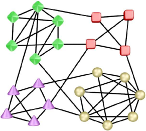
Figure 1: (Color online) The figure illustrates a partition where nodes are separated into distinct communities as indicated by distinct shapes and colors, thus identifying relevant structure in the graph. The current work elaborates on computational transitions and disorder in terms noise (extraneous intercommunity edges) or thermal effects (high temperature $T$ or large system size $N$) of solving such systems using a stochastic heat bath solver (see Appendix D).

We employ a spin-glass-type Potts model Hamiltonian for solving the community detection problem

$$H(\{\sigma\})=-\frac{1}{2}\sum_{i\neq j}\left[A_{ij}-\gamma\left(1-A_{ij}\right)\right]\delta(\sigma_{i},\sigma_{j})$$ (1)

which we refer to as an “Absolute Potts Model” (APM). Given $N$ nodes, $A_{ij}$ denotes the adjacency matrix where $A_{ij}=1$ if nodes $i$ and $j$ are connected and is $0$ otherwise. In general, $A_{ij}$ may be trivially extended to a weighted adjacency matrix $w_{ij}$ (perhaps including “adversarial” relations) Ronhovde and Nussinov (2010), but we utilize unweighted graphs in most of the current work (see Sec. VI). Each spin $\sigma_{i}$ may assume integer values in the range $1\leq\sigma_{i}\leq q$ where $q$ is the (dynamic) number of communities where node $i$ is a member of community $k$ when $\sigma_{i}=k$. In the current work, we set the resolution parameter Ronhovde and Nussinov (2009) to $\gamma=1$ which is near an optimal value for communities with high internal edge densities (see Sec. III).

Previous work Ronhovde and Nussinov (2010, 2009) elaborated on a “zero-temperature” ($T=0$) community detection algorithm which we used to minimize Eq. (1). A depiction of community structure is shown in Fig. 1 where different communities are represented by different node shapes and colors. Here, we investigate the Hamiltonian at non-zero temperatures ($T>0$) by applying a heat bath algorithm (HBA, see Appendix D).

We further invoke $s$ independent solutions (“trials”, see Appendix A) by solving copies of the system which differ by a permutation of the order of the spin indices. This process leads to states that (perhaps locally) minimize Eq. (1), so we select the lowest energy trial as the best solution. We vary $s$ in the range $4\leq s\leq 20$ where we employ $s=4$ trials in general and use $s>4$ trials for calculating the computational susceptibility in Eq. (60).

In our multi-scale (“multiresolution”) analysis, we solve $r=100$ independent “replicas” (see Appendix A) and examine information theory correlations between the replicas and the planted ground state solutions. We schematically show such a set of independent solvers in Fig. 2 where stronger agreement among the replicas indicates a more robust solution. We compute the average inter-replica information correlations among the ensemble of replicas allowing us to infer a more detailed picture of the system beyond that of a single optimized solution. Specifically, information theory extrema as a function of $T$ and $\gamma$ (or other scale parameters in general) correspond to most relevant scale(s) of the system.

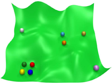
Figure 2: (Color online) The schematic illustrates different minimizers attempting to solve a system. Colored spheres represent distinct minimizers (“replicas”) that seek a (perhaps local) minimum of a cost function. In an easy system, multiple solution attempts will generally reach a good solution (such as the bottom left region of the landscape), but hard systems require more effort to solve accurately (that is, to achieve strong agreement between the replicas). Unsolvable regions restrict accurate solutions without extreme levels optimization (such as exhaustive search).

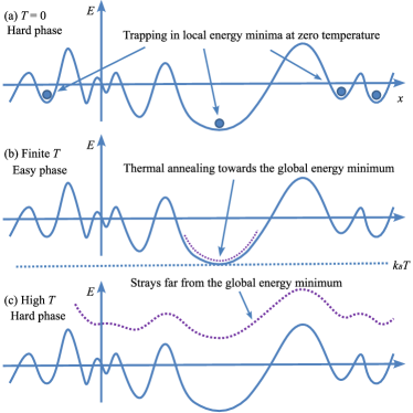
Figure 3: (Color online) Panel (a) schematically illustrates in one dimension the easy and hard phases induced by the level of noise (extraneous intercommunity edges) encountered by a solver. Greedy algorithms are easily trapped in local energy minima above a certain noise threshold. We previously showed that the model of Eq. (1) is robust to noise Ronhovde and Nussinov (2010) even with a greedy algorithm. Stochastic solvers such as a heat bath algorithm (see Appendix D) or simulated annealing enable one to circumvent the effects of some noise, but excessive levels will still thwart these solvers because meaningful partition information is obscured by the complexity of the energy landscape. Panels (b) and (c) schematically depict the easy and hard phases in terms of the temperature for the stochastic heat bath solver (see Appendix D). Above a graph-dependent threshold, the solver is less sensitive to local energy landscape features.

III Construction of embedded graphs and the noise test

Similar to Lancichinetti et al. (2008), we construct a “noise test” benchmark as a medium in which to study phase transitions in random graphs with embedded solutions Ronhovde and Nussinov (2010); Hu et al. (2012a). We define the system “noise” as intercommunity edges that connect a given node to communities other than its original or “best” community assignment. In general Ronhovde and Nussinov (2010), it is not possible at the beginning of an attempted solution to ascertain which edges contribute to noise and which constitute edges within communities of the best partition(s).

For each benchmark graph, we divide $N$ nodes into $q$ communities with a power law distribution of community sizes $\{n_{i}\}$ given by $n^{\beta}$ where $\beta=-1$. We then connect “intracommunity” edges at a high average edge density $p_{in}=0.95$. Initially, the external edge density is zero, $p_{out}=0$, so that we have perfectly decoupled clusters. To this system, we add random intercommunity edges at a density of $p_{out}<0.5$. We define $p_{in}$ ($p_{out}$) as the ratio of the number of intracommunity (intercommunity) edges over the maximum possible intracommunity (intercommunity) edges.

We define the average external degree of each node $Z_{out}$ as the average number of links that a given node has with nodes in communities other than its own. Similarly, the average internal degree $Z_{in}$ is defined as the average number of links to nodes in the same community, and $Z_{in}+Z_{out}=Z$ where $Z$ is the average coordination number. Then we can explicitly write the internal and external edge densities

$$p_{in}=\frac{NZ_{in}}{\sum_{a=1}^{q}n_{a}(n_{a}-1)},$$ (2)

and

$$p_{out}=\frac{NZ_{out}}{\sum_{a=1}^{q}\sum_{b\neq a}^{q}n_{a}n_{b}}.$$ (3)

where $n_{a}$ denotes the size of community $a$.

The communities in this construction are well defined, on average, at reasonable levels of noise ($p_{out}\lesssim 0.3$ depending on the typical community size $n$). As external links are progressively added to the system ($p_{out}$ increases), the communities become increasingly difficult to detect. At some stage, enough noise is added and $p_{out}$ is sufficiently high that the planted partition cannot be detected despite the fact that the optimal ground state is still well-defined. This transition often occurs sharply, particularly for large networks. We investigate the phase transition from the solvable to unsolvable phases at both low and high temperatures by means of the heat bath algorithm described in Appendix D.

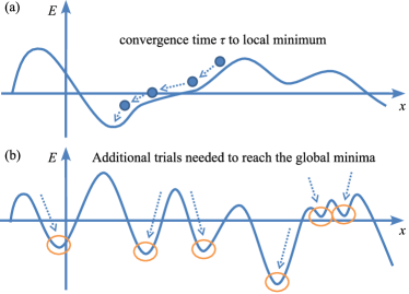
Figure 4: (Color online) The figure schematically illustrates the convergence time of a solver in panel (a) and the effect of additional optimization trials in panel (b). Additional optimization trials are utilized in a “computational susceptibility” $\chi$ in order to numerically estimate the complexity of the energy landscape (see Appendix C).

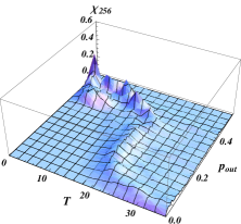
(a)  $N=256$, $q=4$, $\alpha=0.016$

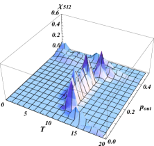
(b)  $N=512$, $q=8$, $\alpha=0.016$

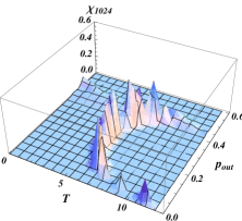
(c)  $N=1024$, $q=16$, $\alpha=0.016$

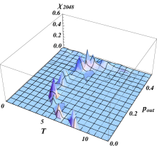
(d)  $N=2048$, $q=32$, $\alpha=0.016$

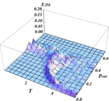
(e)  $N=256$, $q=18$, $\alpha=0.07$

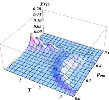
(f)  $N=512$, $q=35$, $\alpha=0.07$

(g)  $N=1024$, $q=70$, $\alpha=0.07$

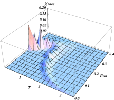
(h)  $N=2048$, $q=140$, $\alpha=0.07$

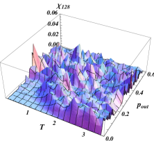
(i)  $N=128$, $q=20$, $\alpha=0.15$

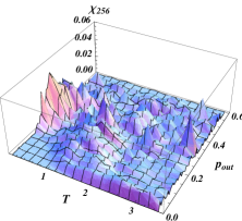
(j)  $N=256$, $q=40$, $\alpha=0.15$

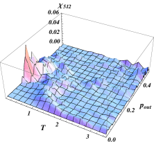
(k)  $N=512$, $q=80$, $\alpha=0.15$

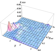
(l)  $N=1024$, $q=160$, $\alpha=0.15$

Figure 5: (Color online) Each panel shows a 3D plot $\chi(T,p_{out})$ as a function of temperature $T$ and noise level $p_{out}$ for systems with the indicated number of nodes $N$, communities $q$, and $\alpha=q/N$ ratio. In panels (a–h) for $\alpha=0.016$ and $0.07$, all plots show three clear phases, and the “ridges” at low and high temperatures mark the hard phase. The hard phase separates the easy phase (the flat region in the lower left corner with low temperature and low noise) from the unsolvable phase (the flat region in the upper right corner with high temperature and high noise). In panels (a)–(h), the ridges in $\chi(T,p_{out})$ become narrower as $N$ increases. The area of the easy (hard) regions decreases (increases) from panel (a) to (d) and (e) to (h), respectively. In panels (a–d) for $\alpha=0.016$, the hard phase at low temperature becomes less prominent from panel (a) to (d), but it becomes more prominent at high temperature. In panels (e–h) for $\alpha=0.07$, the hard phase at low temperature becomes more prominent from panel (e) to (h), but it remains constant at high temperature. In panels (i–l) for $\alpha=0.15$, only the larger systems with $N\geq 512$ show clear phases. The smaller systems with $N=128$ in panel (i) and $N=256$ in panel (j) show very noisy phases where only the easy phase can be readily determined, and the boundaries for the hard and unsolvable phases are difficult to pinpoint.

IV Spin glass type transitions

We previously reported Hu et al. (2012a) on the existence of two spin-glass-type transitions in the constructed graphs mentioned in Sec. III. Evidence for the transitions are observed in several measures such the accuracy of the solution obtained by means of the APM in Eq. (1) (and other models Reichardt and Bornholdt (2006); Ronhovde and Nussinov (2010) in general), the computational effort required to converge to a solution Ronhovde and Nussinov (2009, 2010), entropy effects, and others. Compared to another Potts-type qualtity function Reichardt and Bornholdt (2006) utilizing a “null model” (a random graph used to evaluate the quality of a candidate partition), the APM exhibits a somewhat sharper transition as $N$ is increased Ronhovde and Nussinov (2010). As alluded to above, two transitions are generally encountered as the noise value (or temperature) is increased. At fixed temperature $T$, as $p_{out}$ is steadily increased from zero, the first onset of spin glass behavior first appears for values $p_{1}\leq p_{out}\leq p_{2}$.

Figure 3(a) illustrates a one dimension characterization of the easy and hard phases in terms of the level of noise (extraneous intercommunity edges) encountered by a greedy solver. It is in this context that greedy algorithms are, in general, more easily trapped in local energy minima above a certain noise threshold. Stochastic solvers such a heat bath algorithm discussed in Appendix D or simulated annealing (SA) enable one to circumvent noise to some extent, but excessive levels will even thwart these more robust solvers because meaningful information is eventually obscured by the complexity of the energy landscape. Fig. 3(b,c) depict the easy and hard phases at low and high temperatures $T$, respectively, for our HBA (see Appendix D). Above a graph-dependent threshold, the solver is insensitive to local features, and it is unable to find an accurate solution.

We showed that Eq. (1) is robust to noise Ronhovde and Nussinov (2010) leading to exceptional accuracy even with a greedy algorithm. Some other methods and cost-functions Blondel et al. (2008); Traag et al. (2011) have also proven to be very accurate Lancichinetti and Fortunato (2009) with a greedy-oriented algorithm. While maximizing modularity Newman and Girvan (2004) and a closely related cost function in Reichardt and Bornholdt (2006) have proven to be accurate and productive, Refs. Fortunato and Barthélemy (2007); Good et al. (2010); Lancichinetti and Fortunato (2011) have discussed problems associated with maximizing modularity in community detection. We briefly illustrated Ronhovde and Nussinov (2010) a correspondence between the major transition experienced by Eq. (1) and a Potts model in Reichardt and Bornholdt (2006). We conjecture the existence of a related transition for random knots in Appendix G.

In Sec. IV.1 and IV.2, we elaborate on the transitions using a computational susceptibility $\chi$ as defined in Appendix C. In analogy with other physical susceptibility parameters, $\chi$ measures the response of the system to additional optimization effort. We schematically illustrate the effect in Fig. 4. A higher $\chi$ indicates a more disordered, but navigable, energy landscape where a low $\chi$ indicates that additional optimization has less effect whether due to extreme disorder or a trivially solvable system. Finally in Sec. IV.3, we illustrate the transitions using additional stability measures.

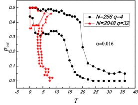
(a)  “hard” phase boundary for $\alpha=0.016$

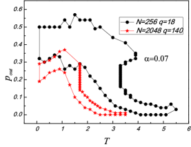
(b)  “hard” phase boundary for $\alpha=0.07$

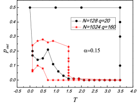
(c)  “hard” phase boundary for $\alpha=0.15$

Figure 6: (Color online) Corresponding to Fig. 5 and Sec. IV.1, each plot depicts the boundaries of the hard phase for the system series with a fixed $\alpha=q/N$ ratio. Panels (a), (b), and (c) show the results for $\alpha=0.016$, $\alpha=0.07$, and $\alpha=0.15$, respectively. System sizes range from $N=256$ to $2048$, and $q$ varies from $4$ to $160$ as indicated in each plot. For each $\alpha$, the area within hard phase boundary becomes progressively narrower indicating that the transitions from the easy to unsolvable phases are more clear in the thermodynamic limit.

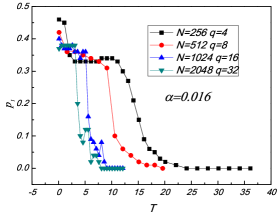
(a)  $p_{1}(T)$ with $\alpha=0.016$

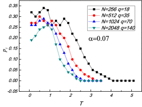
(b)  $p_{1}(T)$ with $\alpha=0.07$

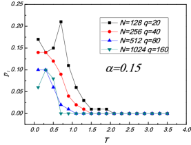
(c)  $p_{1}(T)$ with $\alpha=0.15$

Figure 7: (Color online) Corresponding to Fig. 5 and Sec. IV.1, each plot depicts the first phase transition point $p_{1}$ as a function of the temperature $T$ for systems with a fixed ratio of $\alpha=q/N$. Panels (a), (b), and (c) show the results for $\alpha=0.016$, $\alpha=0.07$, and $\alpha=0.15$, respectively. System sizes range from $N=256$ to $2048$, and $q$ varies from $4$ to $160$ as indicated in each plot. All panels show that when $\alpha$ is fixed, the value of the first transition point $p_{1}$ decreases as the system size increases. This behavior further indicates that the system becomes more complex to solve in the thermodynamic limit.

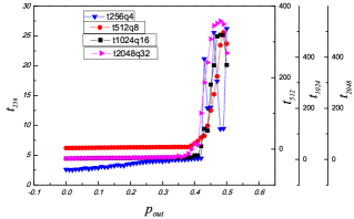
(a)  $\tau$ with $\alpha=0.016$

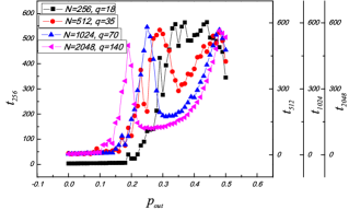
(b)  $\tau$ with $\alpha=0.07$

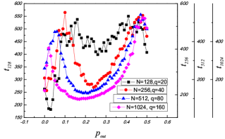
(c)  $\tau$ with $\alpha=0.15$

Figure 8: (Color online) Corresponding to Fig. 5 and Sec. IV.1, the convergence time $\tau$ [see Fig. 4(a)] as a function of noise $p_{out}$ at zero temperature for the systems with a fixed ratio of $\alpha=q/N$. Panels (a), (b), and (c) show the results for $\alpha=0.016$, $\alpha=0.07$ and $\alpha=0.15$, respectively. System sizes range from $N=256$ to $N=2048$, and $q$ varies from $4$ to $160$ as indicates in each plot. The noise level $p_{out}$ at the first peak of the convergence time corresponds to the first transition point $p_{1}$ in Fig. 7 at zero temperature. As the system size increases, the first peak in the convergence time moves to the left. They share the same trend as in Fig. 6 and Fig. 7.

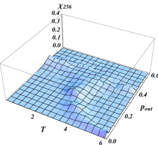
(a)  $N=256$, $q=16$

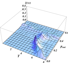
(b)  $N=512$, $q=16$

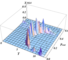
(c)  $N=1024$, $q=16$

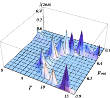
(d)  $N=2048$, $q=16$

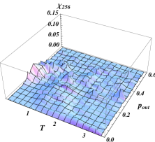
(e)  $N=256$, $q=40$

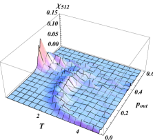
(f)  $N=512$, $q=40$

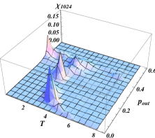
(g)  $N=1024$, $q=40$.

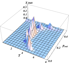
(h)  $N=2048$, $q=40$.

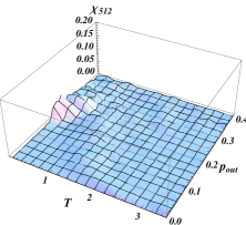
(i)  $N=512$, $q=70$

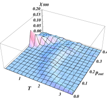
(j)  $N=800$, $q=70$

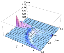
(k)  $N=1024$, $q=70$

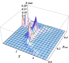
(l)  $N=2048$, $q=70$

Figure 9: (Color online) Similar to Fig. 5, we plot of $\chi(T,p_{out})$ as a function of temperature $T$ and noise level $p_{out}$ for systems with the indicated number of nodes $N$, communities $q$, and $\alpha=q/N$ ratio. Here, $q$ is fixed for each row series, and we vary $\alpha$ (rows) to examine the behavior as $N$ increases (columns). The heights of the susceptibility peaks at higher $T$ increase across each series as $N$ increases whereas the heights at low $T$ are relatively constant. The $N=256$ node systems do not show clear hard or unsolvable phases, but the transitions are strong at high temperature for most panels in the second and third columns of plots.

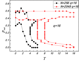
(a)  hard phase boundary for $q=16$

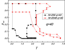
(b)  hard phase boundary for $q=40$

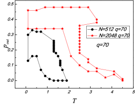
(c)  hard phase boundary for $q=70$

Figure 10: (Color online) Corresponding to Fig. 9 and Sec. IV.2, each plot depicts the boundaries of the hard phase for the system series with a fixed number of communities $q$ where panels (a), (b), and (c) correspond to $q=16$, $40$, and $70$, respectively. System sizes range from $N=256$ to $2048$ as indicated. For each $q$, the area of the hard phase becomes progressively narrower which indicates clearer transitions from the easy to unsolvable phases in the thermodynamic limit.

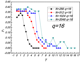
(a)  $p_{1}(T)$ with $q=16$

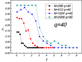
(b)  $p_{1}(T)$ with $q=40$

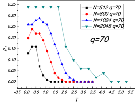
(c)  $p_{1}(T)$ with $q=70$

Figure 11: (Color online) Corresponding to Fig. 9 and Sec. IV.2, each plot depicts the first phase transition point $p_{1}$ as a function of temperature $T$ for systems with a fixed $q$. Panels (a), (b), and (c) show the results for $q=16$, $40$, and $70$, respectively. System sizes range from $N=256$ to $2048$ as indicated in each plot. All panels show that the first transition point increases as the system size increases which is consistent with the complexity trend of the system series.

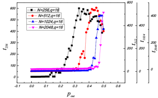
(a)  $\tau$ with $q=16$

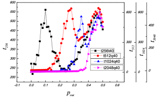
(b)  $\tau$ with $q=40$

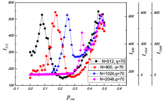
(c)  $\tau$ with $q=70$

Figure 12: (Color online) Corresponding to Fig. 9 and Sec. IV.2, the convergence time $\tau$ [Fig. 4(a)] as a function of noise $p_{out}$ for systems with fixed $q$. Panels (a), (b) and (c) show the results for $q=16$, $40$, and $70$, respectively. System sizes vary from $N=256$ to $2048$ as indicated in each plot. The noise level $p_{out}$ at the first peak of the convergence time corresponds to the initial transition point $p_{1}$ in Fig. 11 at zero temperature. As the system size increases, the first peak in the convergence time moves to the right. They share the same trend as in Figs. 10 and 11.

IV.1 $\chi(T,p_{out})$ at fixed $\alpha=q/N$

We show the phase transitions in terms of three-dimensional (3D) plots with the computational susceptibility $\chi(T,p_{out})$ for a range of system sizes $N$ and numbers of communities $q$. First, we fix the ratio $\alpha=q/N$ and study the phase transitions as $N$ increases. Then we test a range of systems with fixed $q$ as $N$ increases.

IV.1.1 $\chi(T,p_{out})$ at $\alpha=0.016$

In Fig. 5 panels (a) through (d), we begin the analysis at a small $\alpha=q/N=0.016$ ratio. The results for four system sizes are shown: $N=256$, $N=512$, $N=1024$ and $N=2048$ which maintain a fixed ratio of $\alpha$ across the respective rows. Each plot shows the easy, hard, and unsolvable phases.

The two “ridges” in each plot denote the hard phases. The height of the first ridge at low temperature decreases as the system size increases while the height of the second ridge at high temperature increases in the same process. This finite size scaling behavior for the hard phase at high temperature indicates that the phase transition at high temperature exists in the thermodynamic limit. However, the phase transition at low temperature will disappear in the same limit. In the meantime, the ridge in the high temperature will gradually expand into the low temperature region as the system size increases. Thus, for the systems with the small ratio of $\alpha$, the phase transition will exist in almost the entire temperature range in the thermodynamic limit (see Sec. V).

The “easy” phase shrinks and the unsolvable phase expands as $N$ increases. In detail, the approximate area of the easy phase on the left corner in panel (a) is in the range of $T\in(0,20)$ and $p_{out}\in(0,0.4)$. The area of the unsolvable phase on the right upper corner is in the range of $T\in(20,+\infty)$ and $p_{out}\in(0,0.4)$. As the system size increases from $N=256$ in panel (a) to $N=1024$ in panel (c), the area of the easy phase shrinks to the range of $T\in(0,5)$ and $p_{out}\in(0,0.4)$ while the unsolvable phase expands to $T\in(5,+\infty)$ and $p_{out}\in(0,0.4)$. As the system size further increases to $N=2048$ in panel (d), the easy phase further shrinks to the range of $T\in(0,4)$ and $p_{out}\in(0,0.4)$ while the unsolvable phase expands to $T\in(4,+\infty)$ and $p_{out}\in(0,0.4)$. We note that the range of $p_{out}$ for the easy phase does not decrease as the system size increases.

In order to track the range of the hard phases, we further display a set of “boundary” plots in Fig. 6 as well as the first transition point $p_{1}$ as the function of temperature in Fig. 7. For the system series with the fixed $\alpha=0.016$ discussed above, the 2D “hard phase” boundaries and the values of the first transition points are in panel (a) of Fig. 6 and Fig. 7, respectively.

In Fig. 6(a), the area of the hard phase shrinks, and its area at high temperature becomes narrower as the system size increases. Specifically, the width of the hard phase for $N=256$ is about $\Delta T=6$, while it only extends to $\Delta T=1$ for the $N=2048$. Together with the 3D phase diagrams in panels (a)–(d) of Fig. 5, we conclude that the hard phase at the high temperature becomes sharper in the thermodynamic limit.

The boundaries of the hard phase at low temperature are more easily seen in Fig. 7(a) where we plot the first transition point $p_{1}$ as the function of temperature $T$ for a range of systems. The plots confirm the observations in Fig. 5(a)–(d) regarding the constant $p_{out}$ range. That is, the range of $p_{out}$ for the easy phase does not decrease as the system size increases [in Fig. 7(a), $p_{1}$ collapses before $T\leq 5$ for all the systems]. This behavior hints that the first transition point $p_{1}$ at low temperature and small $\alpha$ remains constant in the thermodynamic limit.

As depicted in Fig. 4(a), the convergence time $\tau$ provides another view of the phase transition. We plot $\tau$ as a function of noise level $p_{out}$ in Fig. 8(a) for systems with a fixed ratio of $\alpha=q/N=0.016$. The value $p_{out}$ at the first peak of the convergence time in each system is consistent with the first transition point $p_{1}$ observed in Fig. 7(a). As the system size increases, the peak convergence time shifts to the left, which corresponds to the lower value of $p_{1}$.

IV.1.2 $\chi(T,p_{out})$ at $\alpha=0.07$

For $\alpha=0.07$, the phase transitions are presented in Fig. 5 panels (e) through (h). The phases in panel (e) are noisy compared to panels (f) through (h), and all of the systems are more complicated than the plots with $\alpha=0.016$. As $N$ increases, the phase transitions become more clear. However, contrary to panels (a) through (d), the phase transition at low temperature becomes more prominent as $N$ increases, and the transition at high temperature stays roughly constant. Specifically, the height of the susceptibility peak at low temperature increases from $\chi=0.01$ at $N=256$ in panel (e), $\chi=0.05$ at $N=512$ in panel (f), $\chi=0.1$ for $N=1024$ in panel (g), and finally reaches $\chi=0.2$ in panel (h) with $N=2048$. The phase transitions in this series appear to be persistent.

The easy phase (lower left of each panel) decreases in area as the system size increases. This is the same trend that was observed in the previous $\alpha=0.016$ series implying that the easy phase will tend to decrease in the thermodynamic limit up to a threshold (see Sec. V). Specifically, the easy phase in the smallest system in panel (e) covers the range of $T\in(0,3)$ and $p_{out}\in(0,0.3)$ while in the large system in panel (h) covers $T\in(0,1.5)$ and $p_{out}\in(0,0.2)$. The range for $p_{out}$ in the easy phase decreases as the $N$ increases which differs from the $\alpha=0.016$ data where the noise $p_{out}$ stayed at a roughly constant range of $p_{out}\in(0,0.4)$. In both series for $\alpha=0.016$ and $0.07$, the value of the initial transition point $p_{1}$ decreases in the thermodynamic limit.

The corresponding 2D plots of the hard phase boundaries and the first transition points $p_{1}$ are displayed in Fig. 6(b) and Fig. 7(b), respectively. For the series with $\alpha=0.07$ in Fig. 6(b), the area of the hard phase becomes narrower at both low and high temperatures as the system size increases. In detail, the width of the hard phase for $N=256$ is about $\Delta T=1.3$, while the width shrinks to about $\Delta T=0.3$ at $N=2048$. Together with the 3D phase diagrams in Fig. 5(e)–(h), the phase transitions become sharper in the thermodynamic limit.

As shown in Fig. 7(b), the first transition point $p_{1}$ decreases as the system size increases, even in the low temperature limit. This is consistent with the first peak of the convergence time $\tau$ at zero temperature in Fig. 8(b). This indicates that the system becomes progressively harder to solve in the thermodynamic limit over the whole temperature range.

IV.1.3 $\chi(T,p_{out})$ at $\alpha=0.15$

In panels (i) through (l) of Fig. 5, $\alpha=0.15$ and the clusters are smaller on average resulting in systems that are more difficult to solve. In panels (i) and (j), almost the entire region is covered by small peaks which indicates mixing of the hard and unsolvable phases thus making the phase boundaries hard to detect.

The flat easy regions are recognizable in all panels, but the area is small relative to the previous cases and becomes even smaller as $N$ increases into panel (l). In panel (i), the flat easy region is roughly triangular with legs along $T\in(0,1.5)$ and $p_{out}\in(0,0.2)$. The easy region shrinks to a smaller triangle along $T\in(0,0.2)$ and $p_{out}\in(0,0.2)$ in panel (j) and (k). In panel (l), it further shrinks to $T\in(0,1)$ and $p_{out}\in(0,0.1)$. The easy phase shrinks for both $p_{out}$ and $T$ as $N$ increases which further indicates that the initial transition point $p_{1}$ decreases substantially in the thermodynamic limit.

The corresponding plots of the hard phase boundaries and the first transition points $p_{1}$ are displayed in Figs. 6(c) and 7(c), respectively. From Fig. 6(c), the area of the hard phase shrinks in the thermodynamic limit. The hard phase is more identifiable relative to the unsolvable region as $N$ increases. The initial transition point $p_{1}$ drops as $N$ increases as shown in Fig. 7(c). The convergence time $\tau$ for the systems with the fixed ratio of $\alpha=q/N=0.15$ at zero temperature is shown in Fig. 8(c) where the first peak of $\tau$ shifts to the left as the system size increases. This is consistent with the trend observed in Fig. 7(c). We further show in Fig. 14 and Fig. 15 that the first transition points in “computational susceptibility”, energy, entropy, convergence time and normalized mutual information are consistent with each other.

In Fig. 16, we provide plots of scaled waiting correlation function data which clearly indicate spin glass type collapse. The collapse is best at the center of the computational susceptibility ridge Fig. 16(b). The collapse persists up to the ends of the susceptibility ridge (e.g., $p_{out}=p_{1}$ in Fig. 16(a)) and is no longer valid outside the susceptibility ridge (e.g., $p_{out}=0.26>p_{2}=0.24$ in Fig. 16(c)).

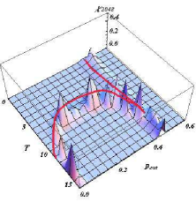
(a)  $\chi(T,p_{out})$ for $q=16$

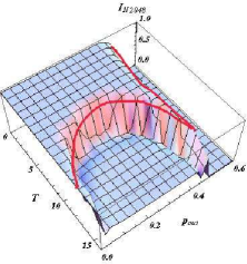
(b)  $I_{N}(T,p_{out})$ for $q=16$

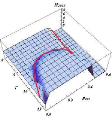
(c)  $H(T,p_{out})$ for $q=16$

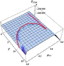
(d)  $E(T,p_{out})$ for $q=16$

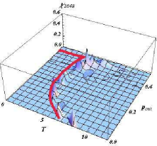
(e)  $\chi(T,p_{out})$ $q=32$

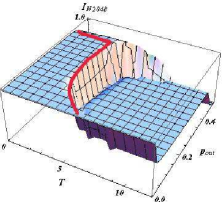
(f)  $I_{N}(T,p_{out})$ for $q=32$

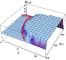
(g)  $H(T,p_{out})$ for $q=32$

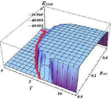
(h)  $E(T,p_{out})$ for $q=32$

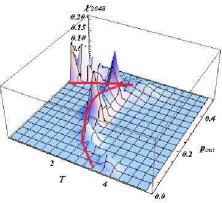
(i)  $\chi(T,p_{out})$ for $q=70$

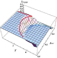
(j)  $I_{N}(T,p_{out})$ for $q=70$

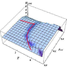
(k)  $H(T,p_{out})$ for $q=70$

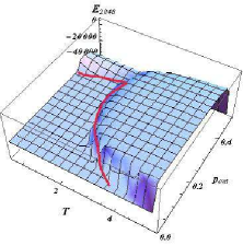
(l)  $E(T,p_{out})$ for $q=70$

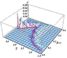
(m)  $\chi(T,p_{out})$ for $q=140$

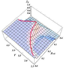
(n)  $I_{N}(T,p_{out})$ for $q=140$

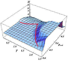
(o)  $H(T,p_{out})$ for $q=140$

(p)  $E(T,p_{out})$ for $q=140$

Figure 13: (Color online) Plots of the computational susceptibility $\chi$ (column one), NMI $I_{N}$ (column two), Shannon entropy $H$ (column three), and energy $E$ (column four) as functions of temperature $T$ and intercommunity noise $p_{out}$. System sizes all use $N=2048$, and $q$ varies from $16$ to $140$ in different rows. All plots show the easy, hard, and unsolvable phases often by rapid shifts in the respective measures. The red lines serve as a guide to the eye for emphasizing the manifestation of the hard phases in each measured quantity where we note that the boundaries match well across each row.

Figure 14: (Color online) The plots of susceptibility $\chi$, convergence time $\tau$, energy $E$, accuracy $I_{N}$ and the Shannon entropy $H$ in terms of noise $p_{out}$ for the system $N=2048$ and $q=140$ at a zero temperature. All the plots show three phases as noise varies: (1) Below $p_{1}=0.2$, the system can be solved in this “easy” region ( e.g., the accuracy is $I_{N}=1$ ); (2) When $0.2<p_{out}<0.24$, where the benefit of extra trials is the largest, it’s “hard” to solve the system without misplacing nodes (e.g., $\chi$, $E$ and $H$ achieve the peak ) ; (3) Above $p_{2}=0.24$, the system is “impossible” to be perfectly solved. $[p_{1},p_{2}]$ are generous bounds in transition crossover regions. Note that the two transitions are demonstrated to be of spin-glass-type by observing the scaling of the correlation function between $[p_{1},p_{2}]$ in Fig. 16.

(a)  $\chi$, $\tau$, $E$, $H$, $I_{N}$ for the system of size $N=1024$

(b)  $I_{N}$ for the system of $N=1024$ with different $q$

Figure 15: (Color online) (a), The plots of susceptibility $\chi$, convergence time $\tau$, energy $E$, accuracy $I_{N}$, Shannon entropy $H$ in terms of noise $p_{out}$ for the system $N=1024$ and $q=70$ at a zero temperature. (b), The normalized mutual information $I_{N}$ in terms of noise $p_{out}$ for a series of systems with the size of $N=1024$ but different number of communities $q$. From both plots, we are able to detect the first and second transition point $p_{1}$ and $p_{2}$. $p_{1}$ is the point where the $I_{N}$ drops from $1$, $\chi$ increases from $0$, $\tau$ achieves the peak, $E$ and $H$ increases from some constant value. $p_{2}$ is the position where the $I_{N}$ curves with different number of communities collapse shown in (b). $p_{2}$ also corresponds to the peak of energy and entropy as shown in (a).

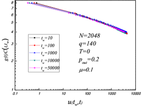
(a)  $p_{out}=0.2$ is within the zero temperature “hard” phase, where the collapse is perfect.

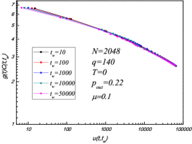
(b)  $p_{out}=0.22$ is within the zero temperature “hard” phase, where the collapse is perfect.

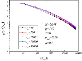
(c)  $p_{out}=0.26$ is within the zero temperature “unsolvable” phase, where the collapse is poor.

Figure 16: (Color online). We show a collapse of the correlation curves for different waiting times $t_{w}$ for a system with $N=2048$ nodes, $q=140$ communities. $p_{out}$ varies from $0.2$ in panel (a) to $0.26$ in panel (c). The first and second transition points for this system are $p_{1}=0.2$ and $p_{2}=0.24$. The temperature is $T=0$. The vertical axis is $g(t)C(t_{w},t)$ where $g(t)=8-\log_{10}(t)$, $C(t_{w},t)=\frac{1}{N}\sum_{i=1}^{N}\delta_{\sigma_{i}(t_{w}),\sigma_{i}(t_{w}+t)}$ is the correlation function. The horizontal axis is $u(t_{w},t)=\frac{1}{1-\mu}[(t+t_{w})^{1-\mu}-t_{w}^{1-\mu}]$ where $\mu=0.1$. The noise $p_{out}=0.2$ (a) and $p_{out}=0.22$ (b) lie within the “hard” region where the collapse of correlation function is perfect. The noise $p_{out}=0.26$ (c) is above the second transition point $p_{2}$ in the “unsolvable” region, where the collapse becomes poor. That the collapse of the correlation function starts to degrade right after the second transition point $p_{2}$ at zero temperature indicates that this transition is of the spin-glass type.

IV.2 $\chi(T,p_{out})$ at fixed $q$

We fix the number of communities at $q=16$, $40$, or $70$ and increase the system size $N$ from $256$ to $2048$. The plots of computational susceptibility $\chi(T,p_{out})$ for $q=16$ series of systems are shown in panels (a) through (d) of Fig. 9. As in Sec. IV.1, the ridges indicate hard phases which become more prominent as $N$ increases while the ridges at low temperature remain at relatively low constant values.

The areas of the easy phases on the lower left corner expand as the system size increases from panel (a) to (d). This trend of increasing area is the reverse of the behavior in the fixed $\alpha$ systems systems in Sec. IV.1. This is easy to understand since, $q$ increases with $N$ here, and the high internal edge density $p_{in}$ causes the larger clusters to be more strongly defined.

We increase the number of communities to $q=40$ for the systems in panels (e) through (h). $N$ varies from $256$ to $2048$, and $\alpha=q/N$ decreases as $N$ increases so that the systems again become less complicated because the communities become more strongly defined. The hard and unsolvable phases in the small $N=256$ system in panel (e) are difficult to distinguish. Only the easy phase can be easily identified by noting the flat region on the lower left of each panel. $\chi(T,p_{out})$ peaks at increasing heights at both the low and high temperatures from panels (f) to (h) indicating that the phase transitions become more prominent as the system size increases.

We further increase the number of communities to $q=70$ and study the phase transitions for the same range of system sizes. The hard phase at high temperature in panel (i) is difficult to detect. $\chi(T,p_{out})$ clearly shows the three phases in panels (j) and (k). The easy phases again become larger as the system size increases. $\chi(T,p_{out})$ in the hard phase increases as $N$ increases indicating that the phase transitions at both low and high temperatures are more obvious from panel (i) to (k).

In Figs. 10 and 11, we also show corresponding 2D plots for the boundaries of the hard phase and the first transition point $p_{1}$ as the function of temperature $T$. In Fig. 10, the area of the hard phase becomes narrower as the system size increases. At $q=40$, for example, the width of the hard phase for the smallest system at $N=256$ is about $\Delta T=1.5$. As $N$ increases, the hard phase width shrinks to $\Delta T=1$ at $N=512$ and down to $\Delta T=0.5$ for $N=2048$ which further indicates that the phase transition becomes sharper in the thermodynamic limit. In Fig. 11, the first transition point $p_{1}$ increases over the entire temperature range as $N$ increases. This behavior is consistent with the system complexity trend as previously mentioned.

In Fig. 12, we further plot the convergence time $\tau$ as the function of noise $p_{out}$ for a fixed number of communities $q$ at zero temperature. $p_{out}$ for the first peak of the convergence time matches the first transition point $p_{1}$ in Fig. 11. As the system size increases, the peak moves to the right. This is also consistent with Fig. 11 where the system becomes less complicated as $N$ increases.

IV.3 Other information theoretic and thermodynamic quantities

We further fortify and provide our results of the phase diagram of our systems as ascertained via other information theoretic and thermodynamics quantities. These measures include the average normalized mutual information $I_{N}$ between replica pairs, Shannon entropy $H$, and energy $E$ as shown in Fig. 13. We additionally show the corresponding computational susceptibility $\chi$ from Fig. 5 or 9 for comparison. All panels are for a system of size $N=2048$. In panels (a) through (d), $q=16$ which corresponds to Fig. 5(d). Panels (e) through (h) plot results for $q=32$ with $\alpha=0.015$ which corresponds to Fig. 9(d). Panels (i) through (l), display the results for $q=70$ which corresponds to Fig. 5(l). Finally, Panels (m) through (p) display results for $q=140$ and $\alpha=0.07$ corresponding to Fig. 9(h).

All panels consistently display the three different complexity phases: the “easy” (flat region, lower left), “hard” (varied central regions), and “unsolvable” phases (far right or top). The existence of the hard phase is reflected by the ridges at both low and high temperatures in the susceptibility $\chi$ plot which often corresponds rapids shifts (up or down) in the other measures. In each plot, the red line serves as a guide to the eye to emphasize the boundaries between different phases. The boundaries are consistent with each other across the respective rows.

In Ref. Hu et al. (2012a), we also demonstrated the spin glass character of the phase transition by observing the exceptional collapse of time autocorrelation curves (over four orders of magnitude of time at high and low temperatures) in the vicinity of the hard phase. We further elucidated on evidence regarding phase transitions Hu et al. (2012a) in identifying community structure via a dynamical approach (some other dynamical methods include Arenas et al. (2006); Gudkov et al. (2008)) where “chaotic-type” transitions that we speculated upon may extend into the node dynamics for large systems.

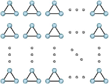
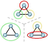
Figure 17: (Color online) Panel (a) depicts $q$ independent cliques (maximally connected clusters). Panel (b) indicates the different combinations of $l=3$ nodes which must be summed (including three copies of the $2$-$1$ configuration) in order to determine the partition function for a single clique.

V non-interacting cliques

As depicted in Fig. 17, we analytically estimate a minimum transition temperature by examining a system with $q$ non-interacting cliques. In panel (a), each of the $q$ communities consists of $l$ nodes which are maximally connected, but no noise exists between these cliques. The presence of noise will, in general, lower the temperature $T_{\times}$ of the transition point which manifests as departure from the easy phase in certain regions of Figs. 5 and 9.

Within our algorithm and model, communities do not interact in an explicit sense. In addition, with this model problem the situation is greatly simplified because no edges are assigned between cliques, so we use Eq. (1) to calculate the partition function of the system by counting the energy contribution of all edges within each cluster over the number of combinations for partitioning the clusters. As a further simplification, we also set the energy contribution for a single edge to be $-2$ so that the Hamiltonian gives an energy of $-1$ for each edge.

V.1 Partition function

First, we investigate the smallest non-trivial clique size with $l=3$ nodes. The partition function for the decoupled cliques is,

$$\mathbf{Z}=\left(\mathbf{Z}_{l}\right)^{q}=\sum_{\sigma_{i},\sigma_{j}}e^{-\beta H_{i,j}}$$ (4)

where $\mathbf{Z}_{l}$ is the partition function for a single clique and $\beta=1/T$ is the inverse temperature. Considering the $l=3$ cluster combinations depicted in Fig. 17(b), $\mathbf{Z}_{3}$ is

$$\mathbf{Z}_{3} = qe^{6\beta}+3q(q-1)e^{2\beta}+3q(q-1)(q-2)$$ (5)

$$+~{}q(q-1)(q-2)(q-3).$$

The first term represents the optimal local cluster solution, and the sum of the remaining terms accounts for the remaining sub-optimal local partitions. We define $\omega_{l}$ as the ratio of Boltzmann weights of the sub-optimal partitions to the optimal solution. For $\mathbf{Z}_{3}$, the ratio $\omega_{3}$ is

$$\omega_{3}=\frac{q(q-1)\left[3e^{2\beta}+3(q-2)+(q-2)(q-3)\right]}{qe^{6\beta}}.$$ (6)

$\omega_{l}<1$ indicates that the optimal solution is dominant, while $\omega_{l}\rightarrow\infty$ means the system is disordered. We can define $\omega_{l}=1$ as the transition point from the ordered phase to the disordered phase, and the corresponding “crossover” temperature $T_{\times}$ is found by solving the transcendental equation

$$3(q-1)e^{-4/T_{\times}}+3(q-1)(q-2)e^{-6/T_{\times}}$$

$$+~{}(q-1)(q-2)(q-3)e^{-6/T_{\times}}=1.$$ (7)

In the limit of large $q$, this equation simplifies to

$$q^{3}e^{-6/T_{\times}}\simeq 1,$$ (8)

which yields our estimate for the crossover temperature

$$T_{\times}\simeq\frac{2}{\log q}$$ (9)

for the $l=3$ clique system.

If we generalize to arbitrary clique size $l$, the corresponding partition function for a single clique becomes

$$\mathbf{Z}_{l} = qe^{2\beta{l\choose 2}}+lq(q-1)e^{2\beta{l-1\choose 2}}$$ (10)

$$+~{}\frac{l(l-1)}{2}q(q-1)(q-2)e^{2\beta{l-2\choose 2}}$$

$$+~{}\cdots+q(q-1)(q-2)\cdots(q-l).$$

Again, the first term in Eq. (10) is the Boltzmann weight of the optimal clique partition, and the other terms sum the weights of the incorrect partitions. $\omega_{l}$ is

$$\omega_{l}=\frac{\sum_{k=1}^{l}{l\choose k}{q\choose k+1}(k+1)!e^{2\beta{l-k\choose 2}}}{qe^{2\beta{l\choose 2}}},$$ (11)

and $\omega_{l}=1$ returns the cross-over temperature $T_{\times}$ for arbitrary cliques of size $l$. We summarize the crossover temperature relations in column one of Table 1 where we express $e^{2/T_{\times}}$ in terms of powers of $q$ for several values of $l$. The general relation is

$$T_{\times}\simeq\frac{l-1}{\log q}.$$ (12)

$l$	$e^{2/T_{\times}}$	$e^{2/T_{\times}^{(1/q)}}$	$e^{2/T_{\times}^{(p)}}$
$2$	$q^{2}$	$q$	$pq^{2}$
$3$	$q$	$q^{2/3}$	$p^{1/3}q$
$4$	$q^{2/3}$	$q^{1/2}$	$p^{1/6}q^{2/3}$
$5$	$q^{1/2}$	$q^{2/5}$	$p^{1/10}q^{1/2}$
$6$	$q^{2/5}$	$q^{1/3}$	$p^{1/15}q^{2/5}$
⋮	⋮	⋮	⋮
$l$	$q^{2/(l-1)}$	$q^{2/l}$	$p^{2/(l^{2}-l)}q^{2/(l-1)}$

Table 1: In column one, the crossover temperature $T_{\times}$ from an “ordered” to a “disordered” state is determined by defining the ratio $\omega_{l}=1$ of the sum of Boltzmann weights of sub-optimal node assignments to the weight of the optimal assignment into clique communities as a function of the cluster size $l$ and the number of communities $q$ in the large $q$ limit. In column two, we estimate $T_{\times}^{(1/q)}\simeq T_{\times}$ through different means by calculating the probability $p=1/q$ that two nodes (in the same clique ideally) are determined to be in the same cluster. In the last column, we generalize column two for an arbitrary probability $p$.

V.2 Symmetry Breaking

We can inquire about the crossover temperature $T_{\times}$ from another perspective. Take two nodes $i$ and $j$ in the same clique. If the probability that a solution assigns them to the same community is high, then the system is in the “ordered” state. If this probability is $1/q$, the system is in its “disordered” phase. We can define a crossover temperature $T_{\times}^{(1/q)}$ at which the probability of node $i$ and $j$ being in the same cluster exceeds $1/q$ and thus symmetry between Potts spins is broken. This probability $P(\sigma_{i}=\sigma_{j})=\langle\delta_{\sigma_{i},\sigma_{j}}\rangle$ is

$$P(\sigma_{i}=\sigma_{j})=\frac{\mbox{Tr}_{\sigma_{i}}\delta_{\sigma_{i},\sigma_{j}}e^{-\beta H}}{\mbox{Tr}_{\sigma}e^{-\beta H}},$$ (13)

where $\sigma_{i}$ and $\sigma_{j}$ denote the cluster memberships for nodes $i$ and $j$, respectively. Expressing the numerator and in terms of $l$ and $q$, Eq. (13) becomes,

$$P(\sigma_{i}=\sigma_{j}) = \Big{\{}qe^{2\beta{l\choose 2}}+(l-2)q(q-1)e^{2\beta{l-1\choose 2}}$$ (14)

$$+~{}\cdots+q(q-1)\cdots(q-l-2)\Big{\}}$$

$$\Big{/}\Big{\{}qe^{2\beta{l\choose 2}}+lq(q-1)e^{2\beta{l-1\choose 2}}$$

$$+~{}\cdots+q(q-1)(q-2)\cdots(q-l)\Big{\}}.$$

In the limit of large $q$, Eq. (14) simplifies to

$$P(\sigma_{i}=\sigma_{j})\simeq\frac{qe^{2\beta{l\choose 2}}+\sum_{k=1}^{l-2}{l-2\choose k}q^{k+1}e^{2\beta{l-k\choose 2}}}{qe^{2\beta{l\choose 2}}+\sum_{k=1}^{l}{l\choose k}q^{k+1}e^{2\beta{l-k\choose 2}}}.$$ (15)

Choosing $P(\sigma_{i},\sigma_{j})=1/q$ yields in a crossover temperature $T_{\times}^{(1/q)}$ at which the system goes from being unbroken q-state symmetry to ordered. When $l=3$, Eq. (15) becomes,

$$q^{2}e^{6\beta}+q^{3}e^{2\beta}\simeq qe^{6\beta}+3q^{2}e^{2\beta}+3q^{3}+q^{4}.$$ (16)

In the large $q$ limit, $e^{2\beta}\simeq q^{2/3}$, and the crossover temperature is $T_{\times}^{(1/q)}=3/\log q$. The asymptotic expressions for several values of $q$ and $l$ are summarized in column two of Table 1. For general $q$ and $l$, the relation is

$$T_{\times}^{(1/q)}\simeq\frac{l}{\log q}.$$ (17)

For a general crossover probability $P(\sigma_{i},\sigma_{j})=p$ with $l=3$, the crossover temperature $T_{\times}^{(p)}$ is determined by solving

$$e^{6\beta}+qe^{2\beta}\simeq pe^{6\beta}+3qpe^{2\beta}+3q^{2}p+q^{3}p.$$ (18)

In the large $q$ limit, Eq. (18) is $e^{2\beta}\simeq p^{1/3}q$, where $T_{\times}^{(p)}\simeq 2/(\log q+1/3\log p)$. Results for $T_{\times}^{(p)}$ for several values of $q$ and $l$ are shown column three of Table 1. For general $q$ and $l$, the relation is

$$T_{\times}^{(p)}\simeq\frac{1}{p^{1/l}q}.$$ (19)

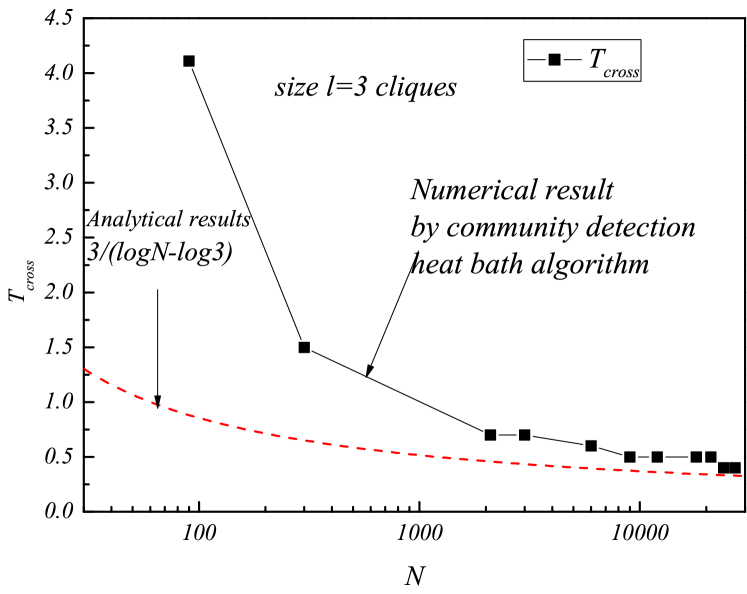
Figure 18: (Color online) The crossover temperature at which the system cannot be perfectly solved as the function of the system size $N$. The data here uses cliques of size $l=3$. The dashed line is the analytical result and the solid line is determined by the heat bath community detection algorithm optimizing the Hamiltonian of Eq. (1).

V.3 Simulated crossover temperature

We can also simulate the crossover temperature $T_{\times}$ or $T_{\times}^{(p)}$ as a function of system size $N$ by solving the non-interacting clique problem using our heat bath community detection algorithm (see Appendix D). As seen in Fig. 18, the simulated and analytic asymptotic behaviors agree well in the large $N$ limit, so the crossover temperature for this trivial system is $T_{\times}=0$.

The crossover temperature derived in this section deals with a heat-induced disorder. That is, it marks the onset of a “liquid” phase that transitions at a lower heat bath temperature as the system size grows. In practice, one uses a SA algorithm that applies a cooling scheme (as opposed to a constant temperature HBA) to improve the attempt at locating the ground state of the system. That is, it applies a high temperature exploration of the general landscape finished by low temperature “fine tuning” of the solution. For the non-interacting cliques in this section, SA would obviously still identify the ground state because the energetic fluctuations would trivially diminish as the system is cooled toward $T=0$.

With increasing $p_{out}$ at low $T$, disorder imposed by the glass-type transition is induced by the complexity of the energy landscape, but the transition is qualitatively comparable in the sense of the induced disorder in the solutions found by the HBA. The glass phase also experiences a transition to a liquid-like disordered state at a temperate that increases slowly with the level of noise, but here, a SA solver will not necessarily transition readily to the ideal solution as the system is cooled because of the inherent complexity of the energy landscape. The greedy algorithm used in Ronhovde and Nussinov (2010) (equivalent to the HBA at $T=0$) applied to the Potts model of Eq. (1) is already very accurate Ronhovde and Nussinov (2009, 2010); Lancichinetti and Fortunato (2009), so we expect that the greatest benefit of SA over a greedy-oriented solver using Eq. (1) will manifest in the hard region near the onset of the “glassy” transition.

(a)  Original

(b)  Easy

(c)  Hard

(d)  Unsolvable

Figure 19: (Reproduced from Ref. Hu et al. (2012b)) We show an image where we apply our community detection algorithm to detect the relevant structures. This case seeks to identify a bird and tree against a sky background. The original images is in panel (a), and the segmentation results are shown in panels (b–d) corresponding to the easy, hard, and unsolvable regions of the community detection problem, respectively. Figure 20 shows the phase diagram identifying these respective regions.

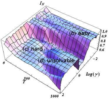
Figure 20: (Reproduced from Ref. Hu et al. (2012b)) We show a three-dimensional phase diagram of NMI ($I_{N}$) versus $\log(\gamma)$ and $\log(T)$ for the image segmentation of the bird in Fig. 19. $T$ is heat bath temperature for a stochastic community detection solver (see Appendix D), and $\gamma$ is the model weight in Eq. (1). We note that the optimal values in the easy and hard regions correspond to the “physical” segmentations of the bird and tree against the background, but the bird is undetectable in the unsolvable region.

V.4 A discussion of the crossover temperature

For a spin system with fixed size $N$, a larger number of spin states $q$ corresponds to a more disordered system. If we expand the partition function of the Potts model in terms of $1/q$, it is explicitly represented as a sum over configurations with progressively larger clusters of identical spins Kasteleyn and Fortuin (1969). That is, two spins with the same index $\sigma_{i}=\sigma_{j}$ are connected. Then three spins $\sigma_{i}=\sigma_{j}=\sigma_{k}$ are connected, etc. The resulting terms illustrate that increasing $q$ emulates increasing temperature $T$.

Our analysis in this section applies to general graphs with ferromagnetic interactions (equivalent to the “label propagation” community detection algorithm Raghavan et al. (2007)) on regular, fixed-coordinate lattices Mercaldo et al. (2004); d’Auriac et al. (2002); Juhász et al. (2001a). Increasing the number of system states $q$ causes the system to be increasingly disordered. Thus, in the community detection problem, increasing number of communities $q$ linearly with the system size $N$ (such that the average community size remains constant), the solvable (easy) phase shrinks to a “small” region as $N\to\infty$.

Figures 13(m–p) illustrate the distinction in the different regions or types of disorder: entropic (high complexity) and energetic (high $T$). Interestingly, in some cases, additional noise emulates a higher temperature solution process in the sense that it provides additional avenues to explore different configurations. Such an effect may occur in Fig. 13(a-d) where the accuracy [$I_{N}$ in panel (b) increases for a short time with increasing noise $p_{out}$].

Fig. 13(n) further shows a crossover region $0.24\lesssim p_{out}\lesssim 0.32$ where mid-range temperatures improve the solution accuracy (higher $I_{N}$). Although this data uses a constant temperature heat bath (no cooling schedule), this is the effect of a stochastic solver (see Appendix D), allowing it to navigate the difficult energy landscape more accurately than a greedy solver. On the left (lower $T$), the more greedy nature of the solver prevents an accurate solution in the presence of high noise. On the right, the higher temperature of the heat bath itself hinders an accurate solution. In effect, the HBA “wanders” at energies above the meaningful, but locally complex, features of the energy landscape resulting in more random solutions.

The results here incorporate a “global” model parameter $\gamma$ in Eq. (1). That is, the model asserts globally optimal $\gamma$(s) for the entire graph. For large graphs, this condition is less likely to be true across the full scope of the network, but one can explore methods to obtain locally optimal $\gamma_{\ell}$ (in time or space) for each region or cluster $\ell$ Ronhovde and Nussinov (2012). Utilizing locally optimal $\gamma_{\ell}$s will likely work to circumvent the temperature transition at low levels of noise. The successful selection of a local $\gamma_{\ell}$ in the glassy (high noise) region is more difficult because of the complex nature of the local energy landscape.

In the following section, we study the free energy of several systems for ferromagnetic Potts models and then generalize to arbitrary weighted Potts models, including antiferromagnetic interactions, on arbitrary graphs Ronhovde et al. (2012).

VI An example of a Phase transition in an image segmentation problem

We illustrate the phase transition effect with an realistic image segmentation example Hu et al. (2012b). In Fig. 19, we apply our community detection algorithm to detect a bird and tree against a sky background. We display the results in Fig. 20 where we plot NMI ($I_{N}$) versus $\log(\gamma)$ in Eq. (1) and $\log(T)$ where $T$ is the temperature for our stochastic community detection solver (see Appendix D). For this problem, we apply edge weights by replacing the $A_{ij}$ elements in Eq. (1) with “attractive” and “repulsive” weights $w_{ij}$ which are defined by regional intensity differences within the image Hu et al. (2012b).

We label the easy (b), hard (c), and unsolvable (d) regions in the phase plot for the bird image in panel (a). Panel (b) shows that our algorithm clearly detects the bird and tree against the background, meaning that the NMI information measure identifies the physically relevant clusters in the problem. In panel (c), the background is segmented separately, but the bird and tree are composed of many small clusters. Panel (d) shows that the bird is undetectable in the unsolvable region.

VII free energy: Simple results

In the following analysis, we explicitly show the large $q$ and large $T$ expansions for the free energy per site in three example systems (a non-interacting clique system, simple interacting clique system, and a random graph) before generalizing the analysis to arbitrary unweighted and weighted graphs. Previous works examined disorder transitions for random-bond Potts models Juhász et al. (2001b); Mercaldo et al. (2005) and Ref. Chang and Shrock (2007) studied zeros of the partition function in the large $q$ limit. Large $q$ behavior was shown to approach mean-field theoretical results on fixed lattices Mittag and Stephen (1974); Pearce and Griffiths (1980). For the unweighted systems, we use a binary distribution for the interaction strength $J=1$ or $0$ (i.e., the energy contribution of an edge is either “on” or “off”).

VII.1 Free energy of a non-interacting clique system under a large $q$ expansion

If we generalize the non-interacting clique system in Fig. 17 to cliques of size $l$, the partition function is

$$\mathbf{Z} = \bigg{[}qe^{\beta J{l\choose 2}}+lq(q-1)e^{\beta J{l-1\choose 2}}$$ (20)

$$+~{}\frac{l(l-1)}{2}q(q-1)(q-2)e^{\beta J{l-2\choose 2}}$$

$$+~{}\cdots+q(q-1)(q-2)\cdots(q-l)\bigg{]}^{q}.$$

When $q\to\infty$,

$$\mathbf{Z} \approx \bigg{[}qe^{\beta J{l\choose 2}}+lq^{2}e^{\beta J{l-1\choose 2}}+\frac{l(l-1)}{2}q^{3}e^{\beta J{l-2\choose 2}}$$ (21)

$$+~{}\cdots+q^{l+1}\bigg{]}^{q}.$$

The free energy per site, $f=-\frac{k_{B}T}{N}\log\mathbf{Z}$, (with the Boltzmann constant set to $k_{B}=1$) is

$$f\approx-T\log q-T\sum_{k=0}^{l-2}\left[{l-1\choose k}\frac{1}{k+1}e^{\beta J{l-1\choose k-1}}\right]q^{-(k+1)}.$$ (22)

From Eq. (22), we further simply the free energy per site

$$f \approx -T\log q-T\sum_{k=0}^{l-2}a(k)e^{\beta J{l-1\choose k-1}}q^{-(k+1)}$$

$$f \approx -T\log q-Ta(0)\frac{e^{\beta J}}{q}$$ (23)

where $a(k)={l-1\choose k}\frac{1}{k+1}$. We will compare Eq. (23) with the high $T$ expansion in the next section. Despite the functional dependence of $\exp(\beta J)$, the large $q$ limit dominates the expansion, forcing the system to be approximately equivalent to a large temperature limit.

VII.2 Free energy of a non-interacting clique system as ascertained from a high temperature expansion

Note that the most ordered Potts graph is a system of non-interacting cliques (maximally connected sub-graphs). That is, the presence of noise (extraneous intercommunity edges) will only serve to increase the overall disorder in the system. One exception is that increased disorder can emulate increased temperature $T$ for both greedy and stochastic community detection solvers (see also Sec. V.4).

We can construct the high $T$ expansion easily by means of Tutte polynomials Welsh and Merino (2000) (see Appendix E.1) where we again solve a system of $q$ cliques of size $l$. Equation (1) and a ferromagnetic Potts model have the same ground state energy for this clique system (see also Secs. VII.5, VII.7, and VII.8 for more general derivations), so the partition function in terms of the Tutte polynomial $t(G;x,y)$ for a graph $G$ is

$$\mathbf{Z}=q^{k(G)}v^{|V|-k(G)}t(G;x,y)$$ (24)

where $q$ is the number of clusters or states, $v=\exp(\beta J)-1$, $G$ denotes the graph, $k(G)$ is the number of connected components in $G$, $|V|=N$ is the number of vertices, $x=(q+v)/v$ and $y=v+1$. For the non-interacting clique system, $k(G)=q$ and $N=lq$. We denote the Tutte polynomial of a single clique of size $l$ as $K_{l}(G;x,y)$.

$K_{2}(G;x,y)=x$, so the partition function is

$$\mathbf{Z} = q^{q}v^{q}x^{q},$$

$$\mathbf{Z} = q^{q}v^{q}\left(\frac{q}{v}+1\right)^{q},$$ (25)

where we used $N=2q$. In a high $T$ approximation, $x\approx q/v\gg 1$, so the partition function becomes $Z\approx q^{2q}$, and the free energy is

$$f\approx-T\log q,$$ (26)

which simply states that the system is completely random in the large $T$ limit.

For triangle cliques, $K_{3}(G;x,y)=x^{2}+x+y$. The graph $G$ is composed of disjoint triangles, so the Tutte polynomial is $t(G;x,y)=\left(x^{2}+x+y\right)^{q}$, and the partition function becomes

$$\mathbf{Z}\approx q^{q}v^{2q}\left(x^{2}+x+y\right)^{q}.$$ (27)

In a high $T$ approximation $y\approx 1$, but $x\approx q/v\gg 1$ in either the large $q$ or large $T$ limits, so we make a further approximation of $y\approx 0$. Then, $K_{3}(G;x,y=0)=x^{q}(x+1)^{q}\approx x^{2q}$. The partition function simplifies to $\mathbf{Z}\approx q^{3q}$, so the free energy per site for $l=3$ is again

$$f\approx-T\log q$$ (28)

which is identical to the $l=2$ result because we consistently applied the approximation $q/v\gg 1$ to $x=(q/v+1)\approx q/v$ and $(x+1)=(q/v+2)\approx q/v$.

Generalizing to an arbitrary clique size $l$ in the high $T$ approximation, the Tutte polynomial $K_{l}(G;x,y=0)$ is

$$K_{l}(G;x,y=0)=\frac{\Gamma\left(x+l-1\right)}{\Gamma\left(x\right)},$$ (29)

The partition function is

$$\mathbf{Z}\approx q^{lq}\left(\frac{v}{q}\right)^{(l-1)q}\frac{\Gamma\left(\frac{q}{v}+l-1\right)}{\Gamma\left(\frac{q}{v}\right)},$$ (30)

and $v=e^{\beta J}-1\approx\beta J$, so the free energy per site yields

$$f\approx-T\log q-\frac{l-1}{l}T\log\left(\frac{\beta J}{q}\right)-\frac{T}{lq}\log\left[\frac{\Gamma\left(\frac{q}{\beta J}+l-1\right)}{\Gamma\left(\frac{q}{\beta J}\right)}\right].$$ (31)

The leading $\log q$ term represents the infinite $T$ limit which is approximately constant in large systems for any clique size $l$. That is, the partition function $\mathbf{Z}_{T\to\infty}\approx q^{N}$ for every system. The $l=2$ and $3$ results above illustrate that when $l\ll q$, the ratio of gamma functions in Eq. (31) simplifies to $x^{lq}$, and the free energy for the non-interacting clique system is approximately $f\approx\log q$ in the large $T$ limit.

The second term in Eq. (31) gives the leading order correction for high $T$. It is absent in the explicit $l=2$ and $3$ results above because we applied the approximation $q/v\gg 1$. Together, the last two terms imply that increasing the temperature $T$ (decreasing $\beta$) emulates increasing the number of communities $q$ for a ferromagnetic Potts model.

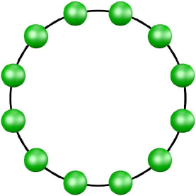
Figure 21: (Color online) A depiction of a circle of cliques (maximally connected clusters) of size $l$ connected by single edges. In contrast to Fig. 17, this system adds a simple interaction between cliques. We analyze the configuration in Sec. VII.3 and show that a ferromagnetic Potts model behaves the same in the large $q$ and large $T$ limits.

VII.3 Free energy for the “circle of cliques” in the high $q$ or the high $T$ expansion

We now investigate the slightly more complicated system depicted in Fig. 21: a “circle of cliques” where each complete sub-graph cluster is connected to its neighbors by a single edge. We construct $q$ cliques of size $l=3$ and apply the Tutte polynomial method Welsh and Merino (2000) to solve the system. As in the previous sub-section, the ground state of Eq. (1) and a ferromagnetic Potts model have the same energy, so we use a ferromagnetic model. In terms of the Tutte polynomial $t(G;x,y)$ for a graph $G$, the partition function is given by Eq. (24).

Equation (74) in Appendix F derives the exact Tutte polynomial for Fig. 21 with $l=3$, and Eq. (76) gives the high $T$ expansion $t(G;x,y=0)=\left(1+x\right)^{q+1}x^{2q-3}$. Substituting $N=3q$ and the approximation $x\approx q/v$ (in either the large $q$ or large $T$ limits), the partition function becomes

$$\mathbf{Z}\approx q^{2q-2}v^{q+2}\left(1+x\right)^{q+1}x^{2q-3}$$ (32)

We factor out $q^{3q}$, and then apply the approximations: $v=\exp(\beta J)-1\approx\beta J$, $x\approx q/v\approx q/(\beta J)\gg 1$, and $q\gg 1$. The free energy per site is then

$$f\approx-T\log q-\frac{2T}{3}\log\left(\frac{q}{\beta J}\right)$$ (33)

As in the previous sub-section, the leading $\log q$ term represents the infinite $T$ limit. Equation (33) affirms the implication of Eq. (31) regarding the corresponding behavior of large $q$ or $T$. Specifically, increasing the temperature (decreasing $\beta$) emulates increasing the number of communities $q$ for a ferromagnetic Potts model.

VII.4 Free energy of a random graph in a large $q$ or a large $T$ expansion

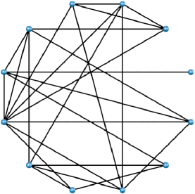
Figure 22: (Color online) A sample depiction of a random graph with $N$ nodes. In Sec. VII.4, we analyze such a system by randomly removing edges from a clique configuration of $N$ nodes under the assumption that we maintain a connected graph. We show that a ferromagnetic Potts model on a random graph behaves the same in the large $q$ and large $T$ limits.

We apply the Tutte polynomial method of Appendix E.1 to determine the high $T$ and high $q$ partition function for a random graph. For calculation purposes, we begin with a complete graph of size $N$. Then we randomly remove edges to construct a random graph such that any two nodes are connected by and edge with a probability $p$. The derivation repeatedly applies lemma 1 stated in Appendix E.1.

We denote the Tutte polynomial of a complete graph (clique) of size $l$ as $K_{l}$. $t(G)$ for a clique with $d$ duplicated edges (multiply defined edges between two nodes) or loops (self-edges) is defined as $K_{l}^{\left(d\right)}$. For economy of notation, we also define $G_{l}^{\left[m\right]}$ as the Tutte polynomial of a graph with $m$ missing edges (i.e., not a clique). Note that $K_{l}^{\left(0\right)}\equiv G_{l}^{\left[0\right]}\equiv K_{l}$. For the following derivation, we work under the assumption that when we delete or contract any edge, the random graph remains connected.

Under the high temperature $T$ or high number of clusters $q$ approximations, $y\ll x$ and $y\simeq 0$. Equation (29) gives the exact expression of the Tutte polynomial $K_{l}(G;x,y=0)$ for a clique at $y=0$. If we cut one edge from the complete graph $K_{N}$, we obtain the recursion formula

$$K_{N} = G_{N}^{\left[1\right]}+K_{N-1}^{\left(N-1\right)},$$

$$K_{N} = G_{N}^{\left[1\right]}+K_{N-1}.$$ (34)

where we applied lemma 1 to obtain Eq. (34). From henceforth, we assume the application of lemma 1. We are interested in the graph with missing edges, so we solve Eq. (34) for $G_{N}^{\left[1\right]}$.

$$G_{N}^{\left[1\right]}=K_{N}-K_{N-1}.$$ (35)

Note that the reduced graph is represented as a summation over complete graphs.

Now we apply the Tutte recursion formula to both sides of Eq. (35).

$$G_{N}^{\left[2\right]}+G_{N-1}^{\left[1\right]}=G_{N}^{\left[1\right]}+K_{N-1}-G_{N}^{\left[1\right]}-K_{N-1}.$$ (36)

We can choose the deleted and contracted edges in the corresponding terms to be identical because the resulting Tutte polynomial is in general independent of the operation order. After collecting terms and substituting the previous $G_{N}^{\left[1\right]}$ result, we solve for $G_{N}^{\left[2\right]}$ to obtain

$$G_{N}^{\left[2\right]}=K_{N}-2K_{N-1}+K_{N-2},$$ (37)

for this particular random graph. Again, the right-hand-side of Eq. (37) is a summation over complete graphs. This recursive relation for $G_{N}^{\left[k\right]}$ continues until we obtain

$$G_{N}^{\left[k\right]}=\sum_{i=0}^{k}(-1)^{i}{k\choose i}K_{N-i}.$$ (38)

We insert this into Eq. (29) with the pre-factor $qv^{N-1}$ to generate the partition function at high $T$

$$\mathbf{Z}=q^{N}\left(\frac{v}{q}\right)^{N-1}\left[\sum_{i=0}^{k}(-1)^{i}{N\choose i}\frac{\Gamma\left(x+N-i-1\right)}{\Gamma\left(x\right)}\right].$$ (39)

We substitute $x=(q+v)/v\approx q/v$ when $v\ll q$ (high $T$ or high $q$ approximations) and again utilize $v=e^{\beta J}-1\approx\beta J$ in the high $T$ approximation to obtain the free energy per site

$$f = -T\log q-\frac{N-1}{N}T\log\left(\frac{\beta J}{q}\right)$$ (40)

$$-\frac{T}{N}\log\left[\sum_{i=0}^{k}(-1)^{i}{N\choose i}\frac{\Gamma\left(\frac{q}{\beta J}+N-i-1\right)}{\Gamma\left(\frac{q}{\beta J}\right)}\right].~{}~{}~{}~{}$$

Note that the first two terms become $\log(q)/N\log(\beta J)$ as $N\to\infty$. From Eq. (40), we obtain the same conclusion for this random graph as for the previously analyzed clique systems. While Secs. VII.1, VII.2, and VII.3 result in free energies with different functional forms, in each case, $q$ and $T$ have the same functional form in the arguments of the functions in the high $T$ limit.

VII.5 Free energy of an arbitrary graph $G$ in the large $T$ expansion

We can construct the explicit high $T$ expansion for an arbitrary (unweighted) graph $G$ by means of the Tutte polynomial method Welsh and Merino (2000). Factoring out $q^{N}$ and substituting $|V|=N$, $x=q/v+1$, and $y=v+1$ in Eq. (24), we write a trivially modified form of the partition function

$$\mathbf{Z}=q^{N}\left[\left(\frac{v}{q}\right)^{N-k(G)}t\left(G;\frac{q}{v}+1,v+1\right)\right].$$ (41)

At this point, the equation is completely general, but the corresponding behavior for temperature $T$ and number of clusters $q$ is almost apparent in the reciprocal relationship of $q$ and $v$.

Again, $x\approx q/v$ in either the large $q$ or large $T$ limits. In a high $T$ approximation, $v\approx\beta J=T/J$ and $y\approx 0$ or $1$ ($y=0$ is a common approximation since $x\gg y$ in the same limit).

$$\mathbf{Z}\approx q^{N}\left[\left(\frac{J}{qT}\right)^{N-k(G)}t\left(G;\frac{qT}{J},y_{\phantom{}{}_{T^{\prime}}}\right)\right]$$ (42)

where $y_{\phantom{}{}_{T^{\prime}}}=0$ or $1$. The free energy per site is then

$$f\approx-T\log q-\frac{N-k(G)}{N}T\log\left(\frac{J}{qT}\right)-\frac{T}{N}\log\left[t\left(\frac{qT}{J},y_{\phantom{}{}_{T^{\prime}}}\right)\right].$$ (43)

The leading $\log q$ term appears in our previous calculations. Again, it represents the infinite $T$ limit for an arbitrary system which is approximately constant in large systems.

From the perspective of increasing $q$, the similarity to the large $T$ behavior is more apparent if we fix the temperature $T=T^{\prime}$ and define an effective interaction constant $J_{q}\equiv e^{J/T^{\prime}}-1$. We then rewrite Eq. (43) as

$$f\approx-T\log q-\frac{N-k(G)}{N}T\log\left(\frac{J_{q}}{q}\right)-\frac{T}{N}\log\left[t\left(\frac{q}{J_{q}},y_{q}\right)\right].$$ (44)

where $y_{q}\equiv e^{J/T^{\prime}}$ is a constant. When $N\to\infty$ and $k(G)\ll N$, the first two terms become $T\log(q)/N\log(\beta J)$. Comparing Eqs. (43) and (44) shows the close correspondence between increasing $q$ (at fixed $T^{\prime}$) and increasing $T$. $J_{q}$ grows exponentially faster than $q$ with decreasing $T^{\prime}$, so a finite (perhaps small) stable or solvable region is likely except in the presence of high noise.

VII.6 Annealed versus quenched averages

The above proofs apply to quenched averages because the binary distribution is constant with respect to the distribution integration. That is, using Eq. (44), we assume a probability distribution $P\left(\{J_{ij}\}\right)$ and integrate over it to obtain the quenched average free energy per site

$$f\left[\{J_{ij}\}\right] = \int DJ_{ij}\prod_{i\neq j}P\left(\{J_{ij}\}\right)\Bigg{\{}\log q$$ (45)

$$+\frac{N-k(G)}{N}\log\left(\frac{J}{qT}\right)$$

$$+\frac{1}{N}\log\left[t\left(\frac{qT}{J},y_{\phantom{}{}_{T^{\prime}}}\right)\right]\Bigg{\}},$$

but the integrand ($f_{0}$) is a constant because $J$ is independent of $\{J_{ij}\}$, so the integral trivially simplifies to

$$f\left[\{J_{ij}\}\right]=f_{0}\int DJ_{ij}\prod_{i\neq j}P\left(\{J_{ij}\}\right).$$ (46)

where the integral is unity. In a more general model with a defined $\{J_{ij}\}$ probability distribution, the leading order $\log q$ contribution would remain unchanged, but we would obtain correction terms from the integration over the quenched interaction distribution $\{J_{ij}\}$.

VII.7 Free energy of non-interacting cliques for an arbitrary weighted Potts model under a large $T$ expansion

We can represent an arbitrary weighted Potts model with ferromagnetic and antiferromagnetic interactions. That is, we can generally write

$$H(\{\sigma\})=-\frac{1}{2}\sum_{i\neq j}\left[a_{ij}A_{ij}-b_{ij}\left(1-A_{ij}\right)\right]\delta(\sigma_{i},\sigma_{j}).$$ (47)

where $a_{ij}$ and $b_{ij}$ are arbitrary “attractive” and “repulsive” edge weights. This summarization includes modularity Newman and Girvan (2004), a Potts model incorporating a “configuration null model” (CMPM) comparison Reichardt and Bornholdt (2006) (the most common variation in Reichardt and Bornholdt (2006) is effectively generalizes modularity), CMPM allowing antiferromagnetic relations Traag and Bruggeman (2009), “label propagation” Raghavan et al. (2007); Barber and Clark (2009), an Erdős-Rényi Potts model Reichardt and Bornholdt (2004, 2006), a “constant Potts model” Traag et al. (2011), the weighted form of the APM Ronhovde and Nussinov (2009, 2010), or a “variable topology Potts model” suggested in Ronhovde and Nussinov (2009).

Note that the repulsive weights $b_{ij}$ are important in that they provide a “penalty function” which enables a well-defined ground state for the Hamiltonian for an arbitrary graph. That is, the ground state of a purely ferromagnetic Potts model in an arbitrary graph is trivially a fully collapsed system (perhaps with disjoint sub-graphs). Several of the above models incorporate a weighting factor $\gamma$ of some type on the penalty term which allows the model to span different scales of the network in qualitatively similar ways.

We denote a the partition function of a graph $G^{*}$ with $l$ nodes and weighted edges $\{e\}$ by $Z(G^{*};q,\mathbf{v})\equiv\mathcal{K}_{l}$. We assume that $J_{e}\ll T$ for all edges $e$, and all pairs of nodes in $G^{*}$ are connected by a weighted edge $J_{e}$ (either ferromagnetic or antiferromagnetic). From Appendix E.2, a recurrence relation for the multivariate Tutte polynomial of a general weighted clique is

$$\mathcal{K}_{l}\approx\left(q+\sum_{k=1}^{l-1}v_{k}\right)\mathcal{K}_{l-1}+O(y_{e}),$$ (48)

The partition function for $\mathcal{K}_{l}$ at high $T$ is

$$\mathcal{K}_{l}\approx q^{N}\prod_{j=2}^{l}\left(1+\sum_{k=1}^{j-1}\frac{v_{k}}{q}\right),$$ (49)

Now, we generate a graph consisting of a set of $q$ non-interacting cliques of size $l_{i}$ where $i=1,2,\ldots,q$.

$$\mathcal{K}_{l}\approx q^{N}\prod_{i=1}^{q}\prod_{j=2}^{l_{i}}\left(1+\sum_{k=1}^{j-1}\frac{\beta J_{k}}{q}\right).$$ (50)

where we used $v_{e}\approx\beta J_{e}$ at high $T$ for general edge weights $J_{e}$ (even if $J_{e}<0$ as long as $J_{e}\ll T$).

The free energy is

$$f \approx -T\log q-\frac{T}{N}\sum_{i=1}^{q}\sum_{j=2}^{l_{i}}\sum_{k=1}^{j-1}\frac{\beta J_{k}}{q}$$ (51)

$$\approx -T\log q-\frac{1}{N}\sum_{i=1}^{q}\frac{E_{i}}{q}$$

$$= -T\log q-\frac{E}{qN}$$

where we invoked $\log(1+x)\approx x$ for $x\ll 1$ there. $E_{i}$ is the energy of cluster $i$ according to the weighted Potts model of Eq. (47), and $E$ is the total energy of the graph. Equations (50) and (51) both imply that large $q$ emulates large $T$ for an arbitrary Potts model on a weighted graph $G$. That is, if a community detection quality function can be expressed in terms of the general Potts model in Eq. (47), then large $q$ and large $T$ are essentially equivalent.

VII.8 Free energy of non-interacting cliques for an arbitrary weighted Potts model under a large $q$ expansion

The multivariate Tutte polynomial Jackson and Sokal (2009) (see also Appendix E.2 and Ref. Ronhovde et al. (2012)) appears in a subgraph expansion over the subset of edges $\mathcal{A}\subseteq\mathcal{E}$ in a graph $G=(V,\mathcal{E})$ with a set of $V$ vertices and $\mathcal{E}$ edges

$$Z(G;q,\mathbf{v})=q^{N}\left[\left(1+\sum_{e^{\prime}=1}^{|\mathcal{E}|}\frac{v_{e^{\prime}}}{q}\right)+\cdots+q^{k(G)-N}\prod_{f^{\prime}=1}^{|\mathcal{E}|}v_{f^{\prime}}\right]$$ (52)

$k(\mathcal{A})$ is the number of connected components of $G_{A}=(V,\mathcal{A})$ and $v_{e}=\exp(\beta J_{e})-1$. For our purposes, Eq. (52) serves as an alternate representation of $Z_{G}$ to facilitate the calculation of the large $q$ expansion.

For large $q$, when $q^{N}\gg|v_{e}|^{L}$, the last term may neglect, and for a system of non-interacting cliques of size $l_{i}$ with $i=1,2,\ldots,q$, the leading order terms in large $q$ are

$$Z(G;q,\mathbf{v})\approx q^{N}\prod_{i=1}^{q}\prod_{j=2}^{l_{i}}\left(1+\sum_{k=1}^{j-1}\frac{v_{k}}{q}\right).$$ (53)

The approximation is identical to Eq. (49) at high $T$. Ref. Ronhovde et al. (2012) calculates an explicit crossover temperature including the last subgraph $\mathcal{A}=\mathcal{E}$ that competes with the large $q$ terms as $T\to 0$. The free energy corresponding to Eq. (53) becomes

$$f \approx -T\log q-\frac{T}{N}\sum_{i=1}^{q}\sum_{j=2}^{l_{i}}\sum_{k=1}^{j-1}\frac{v_{k}}{q}$$ (54)

where we applied the small $x$ approximation $\log(1+x)\approx x$.

In order to illustrate the correspondence in large $q$ and $T$, we fix $T=T^{\prime}$, define $J^{(q)}_{e}\equiv\exp(\beta^{\prime}J_{e})-1$, and rewrite the free energy per site

$$f \approx -T^{\prime}\log q-\frac{T^{\prime}}{N}\sum_{i=1}^{q}\sum_{j=2}^{l_{i}}\sum_{k=1}^{j-1}\frac{J_{k}^{(q)}}{q}.$$ (55)

Large $q$ in Eq. (52) emulates large $T$ in Eq. (50). As with the unweighted case in Eq. (44) in Sec. VII.5, $J_{e}^{(q)}$ is exponentially weighted in $\beta^{\prime}=1/T^{\prime}$, so a non-zero (perhaps small) region of stability is essentially ensured except in the presence of high noise Ronhovde et al. (2012). We can additionally determine a rigorous bound using methods in Batista and Nussinov (2005); Nussinov et al. (2011); Ronhovde et al. (2012)

$$T_{\times}^{\mathrm{UB}}=\frac{\bar{J_{0}}}{\log\left[\frac{p(q-1)}{(1-p)}\right]},$$ (56)

where $\bar{J_{0}}=\frac{1}{2}\sum_{j}J_{j0}\left[1+\mbox{sgn}(J_{j0})\right]$ is a generous upper bound summing only positive energy contributions and $p$ is the probability for finding a given spin $\sigma_{0}$ in a specific spin state $\bar{\sigma}$. This result further agrees with our conclusions. Note that as $p\to 1/q$, the system is completely disordered, so $T_{\times}\to\infty$. As $p\to 1$, the system is perfectly ordered, so $T\to 0$.

VIII Conclusions

We systematically examined the phase transitions for the community detection problem via a “noise test” across a range of parameters. The noise test consists of a structured graph with a strongly-defined ground state. We add increasing numbers of extraneous intercommunity edges (noise) and test the performance of a stochastic community detection algorithm in solving for the well-defined ground state. Specifically, we studied two types (sequences) of systems. In the first such sequence of systems in Fig. 5, we fixed the ratio $\alpha=q/N$ of the number of communities $q$ to the number of nodes $N$. We fixed $q$ at different values and varied $N$ in the second sequence of systems in Fig. 9. In Fig. 13, we explored the largest tested systems with $N=2048$ nodes in more detail where we depicted additional measures to illustrate the transitions. All of these systems showed regions with distinct phase transitions in the large $N$ limit. Deviations occurred most often in smaller systems indicating a definite finite-size effect.

The spin-glass-type phase transitions in our noise test occurred between solvable and unsolvable regions of the community detection problem. A hard, but solvable, region lies at the transition itself where it is difficult, in general, for any community detection algorithm to obtain the correct solution. We analyzed a system of non-interacting cliques and illustrated that in the large $q$ limit, the system experiences a thermal disorder in the thermodynamic limit for any non-zero temperature. When in contact with a heat bath, the asymptotic behavior of the temperatures beyond which the system is permanently disordered varies slowly with the number of communities $q$, specifically, $T_{\times}\simeq O[1/\log q]$. This implies that problems of practical size maintain a definite region of solvability. Given the connection between Jones polynomials of knot theory and Tutte polynomials for the Potts model, our results imply similar transitions in large random knots (see Appendix G).

We further studied the free energy of arbitrary graphs arriving at the same conclusion. Increasing number of communities $q$ emulates increasing $T$ in arbitrary graphs for a general Potts model. The effective interaction strength for increasing $q$ scales such that this disorder is circumvented by the often standard use of a simulated annealing algorithm, but the “glassy” (high noise) region remains a challenge for any community detection algorithm.

Appendix A Definitions: Trials and Replicas

We review the notion of trials and replicas on which our algorithms are based. Both pertain to the use of multiple identical copies of the same system which differ from one another by a permutation of the site indices. Thus, whenever the time evolution may depend on sequentially ordered searches for energy lowering moves (as it will in our greedy algorithm), these copies may generally reach different final candidate solutions. By the use of an ensemble of such identical copies (see, e.g., Fig. 2), we can attain accurate result as well as determine information theory correlations between candidate solutions and infer from these a detailed picture of the system.

In the definitions of “trials” and “replicas” given below, we build on the existence of a given algorithm (any algorithm) that may minimize a given energy or cost function. In our particular case, we minimize the Hamiltonian of Eq.(1.

$\bullet$ Trials. We use trials alone in our bare community detection algorithm. We run the algorithm on the same problem $t$ independent times. This may generally lead to different contending states that minimize Eq.(1). Out of these $t$ trials, we will pick the lowest energy state and use that state as the solution.

$\bullet$ Replicas. We use both trials and replicas in our multi-scale community detection algorithm. Each sequence of the above described $t$ trials is termed a replica. When using “replicas” in the current context, we run the aforementioned $t$ trials (and pick the lowest solution) $r$ independent times. By examining information theory correlations between the $r$ replicas we infer which features of the contending solutions are well agreed on (and thus are likely to be correct) and on which features there is a large variance between the disparate contending solutions that may generally mark important physical boundaries. We will compute the information theory correlations within the ensemble of $r$ replicas. Specifically, information theory extrema as a function of the scale parameters, generally correspond to more pertinent solutions that are locally stable to a continuous change of scale. It is in this way that we will detect the important physical scales in the system (Fig. 2).

Appendix B Information theory and complexity measures

We use information theory measures to calculate correlations between community detection solutions and expected partitions in the noise test problem. To begin, $N$ nodes of partition $A$ are partitioned into $q_{A}$ communities of size $\{n_{a}\}$ where $1\leq a\leq q_{A}$. The ratio $n_{a}/N$ is the probability that a randomly selected node is found in community $a$. The Shannon entropy is

$$H_{A}=-\sum_{a=1}^{q_{A}}\frac{n_{a}}{N}\log_{2}\frac{n_{a}}{N}$$ (57)

The mutual information $I(A,B)$ between partitions $A$ and $B$ is

$$I(A,B)=\sum_{a=1}^{q_{A}}\sum_{b=1}^{q_{B}}\frac{n_{ab}}{N}\log_{2}\frac{n_{ab}N}{n_{a}n_{b}}$$ (58)

where $n_{ab}$ is the number of nodes of community $a$ in partition $A$ that are also found in community $b$ of partition $B$. The normalized mutual information $I_{N}(A,B)$ is then

$$I_{N}(A,B)=\frac{2I(A,B)}{H_{A}+H_{B}}.$$ (59)

with the obvious range of $0\leq I_{N}(A,B)\leq 1$. High $I_{N}$ values indicate better agreement between compared partitions.

Appendix C Computational susceptibility

The complexity $\Sigma(e)$ of the energy landscape is related to the number of states ${\cal{N}}(E)\sim\exp[N\Sigma(e)]$ Mézard et al. (2002) with energy $E$ and energy density $e=E/N$. In the current analysis, we detect the onset of the high complexity with no prior assumptions or approximations by computing a “computational susceptibility” Ronhovde and Nussinov (2009) defined as

$$\chi_{n}=I_{N}(s=n)-I_{N}(s=4).$$ (60)

That is, $\chi$ measures the increase in the normalized mutual information $I_{N}$ as the number of trials (number of independently solved starting points in the energy landscape) $s=n$ is increased. Physically, we evaluate how many different optimization trials are necessary to achieve a desired accuracy threshold.

$\chi$ evaluates the expected response of the system to additional optimization effort. That is, a higher $\chi$ indicates that additional optimization effort will likely result in a better solution. A low value of $\chi$ indicates that there will be less improvement from the additional effort whether due to a trivially solvable system, a complex energy landscape with numerous local minima that trap the solver (at low to moderate temperatures), or thermal-oriented effects of randomly wandering the energy landscape.

Appendix D Heat Bath Algorithm

We extend the greedy algorithm in Ronhovde and Nussinov (2010, 2009) to non-zero temperatures by applying a heat bath algorithm. After, we connect the system to a large thermal reservoir at a constant temperature T, the probability for a particular node to move from community $a$ to $b$ is set by a thermal distribution Reichardt and Bornholdt (2006),

$$p_{a\to b}=\frac{\exp(-\Delta E_{a\to b}/T)}{\sum_{d}\exp(-\Delta E_{a\to d}/T)}.$$ (61)

$\Delta E_{a\rightarrow b}$ is the energy change that results if the node is moved to the new community $b$, and the index $d$ runs over all connected clusters including its current community or a new empty community. The steps of our heat bath algorithm are as follows:

($1$) Initialize the system. Initialize the network into a “symmetric” state by assigning each node as the lone member of its own community (i.e., $q_{0}=N$).

($2$) Find the best cluster for node $i$. Select a node and determine to which clusters it is connected (including its current community and an empty cluster). Calculate the energy change $\Delta E_{a\to b}$ required to move to each connected cluster $b$. Calculate and sum all Boltzmann weights. Generate a random number between $0$ and $1$ and determine into which cluster the node is placed.

($3$) Iterate over all nodes. Repeat step $2$ in sequence for each node.

($4$) Merge clusters. Allow for the merger of community pairs based on the same Boltzmann-weighted merge probabilities.

($5$) Repeat the above two steps. Repeat steps $2$ through $4$ until the maximum number of iterations is reached.

($6$) Repeat all the above steps for s trials. Repeat steps $1$–$5$ for $s$ trials and select the lowest energy trial as the best solution. Each trial randomly permutes the order of nodes in the initial state.

This HBA is similar to our greedy algorithm except that we use a random process to select the node moves in steps (2) and (4). The results obtained at low temperature by our HBA are very close to the results obtained by the zero temperature greedy algorithms. Note that there is no cooling scheme as occurs in SA, so step $5$ ends at a maximum number of iterations as opposed to a unchanged best partition that is achieved as $T\to 0$ in SA.

In the easy phase, different starting trajectories, each beginning in the symmetric initial state, but they often lead to the same solution. In the hard phase, changing the random seed may significantly alter the final result of an individual trial because the solver becomes trapped in different local minima. Thus we apply additional trials in order to sample different regions of the energy landscape and arrive at better solutions. In the unsolvable phase, increasing the number of trials $s$ does not substantially change the quality of the solutions unless one happens to sample the energy landscape in the immediate vicinity near the optimal partition, but the probability of doing so is small with a finite number of trials $s$.

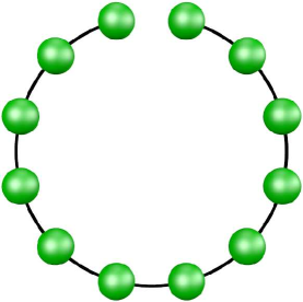
Figure 23: (Color online) In panel (a), we depict a chain $B_{q}$ of $q$ cliques (complete sub-graphs of maximally connected clusters) of size $l$ connected by single edges. The corresponding circle of $q$ cliques $C_{q}$ is depicted in Fig. 21. In panel (b), we show the derivation of the Tutte polynomial in Eq. (72) for size $l=3$ cliques. We iteratively break edges and merge nodes according to the Tutte polynomial recurrence relation Welsh and Merino (2000) in Appendix E.1 until we arrive at configurations that are reduced clique circle components. For presentation purposes, gray edges are cut in the next line of the derivation. The dashed gray line at the bottom of each sub-graph represents the remainder of the clique circle which is not touched or affected by the operations on the displayed subgraph.

Appendix E Tutte polynomials

We give a very brief introduction to Tutte polynomials consisting of the essential facts necessary for the derivations presented in this paper. The notation used here is mostly standard, but the notation elsewhere in the text deviates from standard notation in order to facilitate the partition function derivation in Sec. VII.4. For an undirected graph $G$, we denote the deletion (removal) of an edge $e$ by $G^{\prime}$ and a contraction of the edge by $G^{\prime\prime}$ where a contraction consists of removing the edge $e$ and merging the corresponding vertices.

E.1 Unweighted graph $G$

If $G$ has no edges, the Tutte polynomial is $t(G;x,y)=1$. If $G$ is a disjoint graph of partitions, then $A$ and $B$ $t(G;x,y)=t(A;x,y)~{}\!t(B;x,y)$. When an edge $e$ in an unweighted graph $G$ is “cut,” the recurrence relations are Welsh and Merino (2000):

• For a general edge, $t(G;x,y)=t(G_{e}^{\prime};x,y)+t(G_{e}^{\prime\prime};x,y)$ which is the sum of two graphs where $e$ is deleted and contracted.

• If edge $e$ is an isthmus between two otherwise disconnected regions of $G$, then $t(G;x,y)=x~{}\!t(G_{e}^{\prime\prime};x,y)$ where the edge $e$ is contracted.

• If edge $e$ is a loop (a vertex self-edge), then $t(G;x,y)=y~{}\!t(G_{e}^{\prime};x,y)$ where the edge $e$ is deleted.

The resulting Tutte polynomial is a function of two variables $(x,y)$, and it is independent of the construction order. Different graphs $G$ and $H$ may be described by the same function $t(G;x,y)=t(H;x,y)$. A sample calculation is performed Appendix F for a circle of complete sub-graphs (cliques) as shown in Fig. 23(b).

Tutte polynomials are related to the partition function of a ferromagnetic ($J>0$) or antiferromagnetic ($J<0$) Potts model given by

$$H(\{\sigma\})=-\sum_{i\neq j}J\delta(\sigma_{i},\sigma_{j})$$ (62)

for any connected pair of nodes $i$ and $j$ with an interaction strength $J$. The corresponding partition function is

$$Z=q^{k(G)}v^{|V|-k(G)}t(G;x,y)$$ (63)

where $q$ is the number of clusters or states, $v=\exp(\beta J)-1$, $G$ denotes the graph, $k(G)$ is the number of connected components in $G$, $|V|$ is the number of vertices, $x=(q+v)/v$ and $y=v+1$.

In Sec. VII.4, we use the following lemma to derive high temperature $T$ approximation for a constructed random graph. We denote $K_{l}$ as the Tutte polynomial for a complete graph, and $K_{l}^{(d)}$ denotes that the graph has $d$ duplicated (possibly redundant) edges.

Lemma 1.

For a clique $K_{l}^{(d)}$ of size $l$ with $d$ duplicate edges between any pair of nodes, the Tutte polynomial at $y=0$ is $K_{l}$.

Proof.

Let $G$ be a complete graph with $l$ vertices and $d=1$ redundant edge. If we delete and contract the duplicate edge, the Tutte polynomial $t(G)\equiv K_{l}^{(d=1)}$ is

$$K_{l}^{(1)}=K_{l}+K_{l-1}^{(l-1)}$$

The contracted vertex in the second term contains $r=1$ loop. We cut the loop and have

$$K_{l}^{(1)} = K_{l}+yK_{l-1}^{(l-2)}$$

$$K_{l}^{(1)} = K_{l}$$ (64)

where we used $y=0$ in the second line.

Now, assume that we can reduce $K_{l}^{(d)}=K_{l}$. Let $G$ be a complete graph with $l$ vertices and $d+1$ duplicate edges. If we cut one duplicate edge, the resulting Tutte polynomial $t(G)\equiv K_{l}^{(d+1)}$ is

$$K_{l}^{(d+1)}=K_{l}^{(d)}+K_{l-1}^{(d+l-1)}$$

The contracted vertex in the second term contains $r\geq 1$ loops. We cut each loop in sequence and obtain

$$K_{l}^{(d+1)} = K_{l}^{(d)}+y^{r}K_{l-1}^{(d+l-r-1)}.$$

$$K_{l}^{(d+1)} = K_{l}^{(d)}$$ (65)

Since $K_{l}^{(d)}=K_{l}$, we also equate $K_{l}^{(d+1)}=K_{l}$ by Eq. (65). Equation (64) shows that the relation holds for $d=1$; therefore, by mathematical induction $K_{l}^{(d)}=K_{l}$ holds true for any integer $d\geq 1$.∎

E.2 Weighted graph $G$

An excellent summary of multivariate Tutte polynomials (MVTP) is found in Ref. Jackson and Sokal (2009). The MVTP allows for arbitrary weights $\mathbf{v}=[v_{e}]$ for the edges $\{e\}$ of $G$. If $G$ has no edges, the MVTP is $Z(G;q,\mathbf{v})=q$. For an undirected graph $G$, the weighted Potts Hamiltonian is

$$H(\{\sigma\})=-\sum_{i\neq j}J_{ij}\delta(\sigma_{i},\sigma_{j}).$$ (66)

When an edge $e$ in $G$ is “cut,” the recurrence relation is

$$Z(G;q,\mathbf{v})=Z(G^{\prime};q,\mathbf{v})+v_{e}Z(G^{\prime\prime};q,\mathbf{v})$$ (67)

where $J_{e}$ corresponds to the edge weight between two nodes $i$ and $j$ and $v_{e}=\exp{\beta J_{e}}-1$.

As with the unweighted case, if $G$ is a disjoint graph of partitions $A$ and $B$, then $Z(G;x,y)=Z(A;q,\mathbf{v})~{}\!Z(B;q,\mathbf{v})$. If partitions $A$ and $B$ are joined at a single vertex, then then $Z(G;x,y)=Z(A;q,\mathbf{v})~{}\!Z(B;q,\mathbf{v})/q$. Unlike Eq. (63) for unweighted graphs, Eq. (67) holds for loops or bridges, but for concreteness, cutting an isthmus $e$ yields

$$Z(G;q,\mathbf{v}) = \left(1+v_{e}/q\right)Z(G_{e}^{\prime};x,y)$$ (68)

$$Z(G;q,\mathbf{v}) = \left(q+v_{e}\right)Z(G_{e}^{\prime\prime};x,y)$$ (69)

where $e$ is deleted or contracted, respectively. If $e$ is a loop, then

$$Z(G;q,\mathbf{v})=(1+v_{e})Z(G_{e}^{\prime};x,y).$$ (70)

Note that the MVTP is the partition function. That is, there are no prefactors of $q$ or $v_{e}$. Finally, if two parallel edges connect the same pair of nodes $i$ and $j$ with weights $J_{1}$ and $J_{2}$, then $Z_{G}$ is unchanged if we replace the parallel edges by a single edge with a weight $J^{\prime}=J_{1}+J_{2}$ (this negates the need for lemma 1 above).

Appendix F Derivation of the Tutte polynimial for a circle of cliques

As depicted in Fig. 21, we define $C_{q}$ as a circle of $q$ cliques where we focus those of size $l=3$ for the current derivation. The Tutte polynomial for a triangle is $\Delta\equiv\left(x^{2}+x+y\right)$. For convenience, we also define, $\Delta^{\prime}\equiv(\Delta+x+1)=[(x+1)^{2}+y]$ and $y^{\prime}\equiv(x+y+1)$.

We define $B_{q}$ to be the Tutte polynomial for a clique chain as depicted in Fig. 23(a). In this case, it is trivial to construct $B_{q}$

$$B_{q}=x^{q-1}\left(x^{2}+x+y\right)^{q}.$$ (71)

With Eq. (71), we construct a recurrence relation for the clique circle configurations as shown in Fig. 23(b)

$$C_{q}=B_{q}+x\left(x+1\right)B_{q-1}+\left(x+y+1\right)C_{q-1}.$$ (72)

From this relation, we can sum the series exactly.

$$C_{q} = B_{q}+\Delta^{\prime}B_{q-1}+x\left(x+1\right)\left(x+y+1\right)B_{q-2}$$

$$+~{}\left(x+y+1\right)^{2}C_{q-2}$$

$$\vdots \phantom{B_{q}+\Delta^{\prime}B_{q-1}}\vdots$$

$$C_{q} = B_{q}+\Delta^{\prime}\sum_{i=0}^{q-4}\left(x+y+1\right)^{i}B_{q-i-1}$$ (73)

$$+~{}\Delta\left(x+y+1\right)^{q-3}B_{2}+\left(x+y+1\right)^{q-2}C_{2}.~{}~{}~{}~{}~{}$$

Note that the last $B_{j}$ term uses $\Delta$ not $\Delta^{\prime}$. Also, it can be shown that $C_{2}=\left(x+1\right)^{2}\big{(}x^{3}+\Delta\big{)}+y\left(x+1\right)\Delta$. Substituting these values into the equation, we arrive at

$$C_{q} = x^{q-1}\Delta^{q}+\Delta^{\prime}\sum_{i=0}^{q-4}{y^{\prime}}^{i}x^{q-i-2}\Delta^{q-i-1}+x{y^{\prime}}^{q-3}\Delta^{3}$$ (74)

$$+~{}x{y^{\prime}}^{q}\big{(}x^{2}+x+1\big{)}+y{y^{\prime}}^{q-1}\Delta^{\prime}.$$

In the high temperature $T$ limit, $y\ll x$, so we approximate $y\simeq 0$, and the equation simplifies to

$$C_{q}^{(T)} \simeq x\left(x+1\right)^{q}\Big{[}x^{2q-2}+\cdots+x^{2}+x+1\Big{]}$$ (75)

$$= x\left(x+1\right)^{q}\left[\frac{1-x^{2q-1}}{1-x}\right],$$

We make a final high $T$ approximation

$$C_{q}^{(T)}\simeq\left(x+1\right)^{q+1}x^{2q-3}$$ (76)

using $\left(x^{2q-1}-1\right)\simeq x^{2q-1}$ and $\left(1-x\right)^{-1}\simeq\left(1+x\right)/x^{2}$.

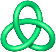
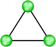
Figure 24: (Color online) Panel (a) depicts the trefoil knot, and panel (b) shows the corresponding graph $G$ constructed from the distinct knot regions and crossings Kauffman (1989). That is, nodes correspond to “checkerboard-shaded” regions (shade the outside lobes of the trefoil knot leaving the interior region unshaded), and edges correspond to knot crossings. Jones polynomials $V_{J}(x)$ in knot theory are related to Tutte Polynomials, and Eq. (77) represents the trefoil knot corresponding to the triangle subgraph in panel (b).

Appendix G Random knot “transitions”

A general 3D knot may be represented as a $4$-valent planar graph Kauffman (1989) [i.e., corresponding to a two-dimensional (2D) square lattice connectivity allowing self-loops]. This relation connects the Tutte polynomial to the Jones polynomial in knot theory. Conversely, all connected, signed planar graphs have a corresponding link diagram representation (2D knot projection). Alternating over-under crossings result in unsigned planar graphs Kauffman (1989) (e.g., the trefoil knot in Fig. 24). Ref. Kauffman (2005) provides an introduction to the mathematics and physics of knot theory. The Jones polynomial of a given knot is intimately related to quantum field theories Witten (1989), via its connection to [an SU(2) type] Wilson loop associated the same knot.

As a concrete example, Fig. 24(a) depicts a simple trefoil knot which is related to the triangle clique depicted in Fig. 24(b) Kauffman (1989). The Tutte polynomial of Fig. 24(b) is $K_{3}(G;x,y)=x^{2}+x+y$. Then we generate the Jones polynomial

$$V_{J}(x)=x^{2}+x+\frac{1}{x}$$ (77)

where we used $xy=1$ because the trefoil knot has alternating crossings Thistlethwaite (1987). While the trefoil knot is clearly not random, we conjecture that the transitions detected in random graphs with embedded ground states in the current work can have similar transition repercussions in random knots.

References

- Newman (2008) M. E. J. Newman, Phys. Today 61, 33 (2008).
- Fortunato (2010) S. Fortunato, Phys. Rep. 486, 75 (2010).
- Rosvall and Bergstrom (2008) M. Rosvall and C. T. Bergstrom, Proc. Natl. Acad. Sci. U.S.A. 105, 1118 (2008).
- Blondel et al. (2008) V. D. Blondel, J.-L. Guillaume, R. Lambiotte, and E. Lefebvre, J. Stat. Mech.: Theory Exp. 10, P10008 (2008).
- Hastings (2006) M. B. Hastings, Phys. Rev. E 74, 035102(R) (2006).
- Reichardt and Bornholdt (2006) J. Reichardt and S. Bornholdt, Phys. Rev. E 74, 016110 (2006).
- Lancichinetti et al. (2009) A. Lancichinetti, S. Fortunato, and J. Kertész, New J. Phys. 11, 033015 (2009).
- Ronhovde and Nussinov (2009) P. Ronhovde and Z. Nussinov, Phys. Rev. E 80, 016109 (2009).
- Cheng and Shen (2010) X.-Q. Cheng and H.-W. Shen, J. Stat. Mech.: Theory Exp. 2010, P04024 (2010).
- Gudkov et al. (2008) V. Gudkov, V. Montealegre, S. Nussinov, and Z. Nussinov, Phys. Rev. E 78, 016113 (2008).
- Barber and Clark (2009) M. J. Barber and J. W. Clark, Phys. Rev. E 80, 026129 (2009).
- Danon et al. (2005) L. Danon, A. Díaz-Guilera, J. Duch, and A. Arenas, J. Stat. Mech.: Theory Exp. 9, P09008 (2005).
- Noack and Rotta (2009) A. Noack and R. Rotta, in Experimental Algorithms, edited by J. Vahrenhold (Springer-Verlag Berlin, Heidelberg, 2009), vol. 5526, pp. 257–268.
- Shen and Cheng (2010) H.-W. Shen and X.-Q. Cheng, J. Stat. Mech.: Theory Exp. 2010, P10020 (2010).
- Lancichinetti and Fortunato (2009) A. Lancichinetti and S. Fortunato, Phys. Rev. E 80, 056117 (2009).
- Hogg et al. (1996) T. Hogg, B. A. Huberman, and C. P. Williams, Artificial Intelligence 81, 1 (1996).
- Mézard et al. (2002) M. Mézard, G. Parisi, and R. Zecchina, Science 297, 812 (2002).
- Monasson et al. (1999) R. Monasson, R. Zecchina, S. Kirkpatrick, B. Selman, and L. Troyansky, Nature (London) 400, 133 (1999).
- Mertens (1998) S. Mertens, Phys. Rev. Lett. 81, 4281 (1998).
- Gent and Walsh (1996) I. P. Gent and T. Walsh, Artificial Intelligence 88, 349 (1996).
- Weigt and Hartmann (2000) M. Weigt and A. K. Hartmann, Phys. Rev. Lett. 84, 6118 (2000).
- Lacasa et al. (2008) L. Lacasa, B. Luque, and O. Miramontes, New J. Phys. 10, 023009 (2008).
- Krzakala and Zdeborová (2008) F. Krzakala and L. Zdeborová, Journal of Physics: Conference Series 95, 012012 (2008).
- Bauke et al. (2003) H. Bauke, S. Mertens, and A. Engel, Phys. Rev. Lett. 90, 158701 (2003).
- Mukherjee and Manna (2005) G. Mukherjee and S. S. Manna, Phys. Rev. E 71, 066108 (2005).
- Arévalo et al. (2010) R. Arévalo, I. Zuriguel, and D. Maza, Phys. Rev. E 81, 041302 (2010).
- Ashok and Patra (2010) B. Ashok and T. K. Patra, Pramana 75, 549 (2010).
- Rose et al. (1990) K. Rose, E. Gurewitz, and G. C. Fox, Phys. Rev. Lett. 65, 945 (1990).
- Graepel et al. (1997) T. Graepel, M. Burger, and K. Obermayer, Phys. Rev. E 56, 3876 (1997).
- Dorogovtsev et al. (2008) S. N. Dorogovtsev, A. V. Goltsev, and J. F. F. Mendes, Rev. Mod. Phys. 80, 1275 (2008).
- Ronhovde and Nussinov (2010) P. Ronhovde and Z. Nussinov, Phys. Rev. E 81, 046114 (2010).
- Hu et al. (2012a) D. Hu, P. Ronhovde, and Z. Nussinov, Phil. Mag. 92, 406 (2012a).
- Good et al. (2010) B. H. Good, Y.-A. de Montjoye, and A. Clauset, Phys. Rev. E 81, 046106 (2010).
- Decelle et al. (2011) A. Decelle, F. Krzakala, C. Moore, and L. Zdeborová, Phys. Rev. Lett. 107, 065701 (2011).
- Lee et al. (2005) E. J. Lee, K.-I. Goh, B. Kahng, and D. Kim, Phys. Rev. E 71, 056108 (2005).
- Moreno et al. (2003) Y. Moreno, R. Pastor-Satorras, A. V zquez, and A. Vespignani, Europhys. Lett. 62, 292 (2003).
- Wang and Chen (2008) W.-X. Wang and G. Chen, Phys. Rev. E 77, 026101 (2008).
- Zheng et al. (2007) J.-F. Zheng, Z.-Y. Gao, and X.-M. Zhao, Europhys. Lett. 79, 58002 (2007).
- Wu et al. (2006) J.-j. Wu, Z.-y. Gao, and H.-j. Sun, Phys. Rev. E 74, 066111 (2006).
- Ikeda et al. (2010) Y. Ikeda, T. Hasegawa, and K. Nemoto, Journal of Physics: Conference Series 221, 012005 (2010).
- Tahbaz-Salehi and Jadbabaie (2007) A. Tahbaz-Salehi and A. Jadbabaie, in Proceedings of the 2007 American Control Conference (IEEE, 2007), pp. 699–704.
- Arenas et al. (2006) A. Arenas, A. Díaz-Guilera, and C. J. Pérez-Vicente, Phys. Rev. Lett. 96, 114102 (2006).
- Serrano and Boguñá (2006) M. Á. Serrano and M. Boguñá, Phys. Rev. Lett. 97, 088701 (2006).
- Moore and Newman (2000) C. Moore and M. E. J. Newman, Phys. Rev. E 61, 5678 (2000).
- Lancichinetti et al. (2008) A. Lancichinetti, S. Fortunato, and F. Radicchi, Phys. Rev. E 78, 046110 (2008).
- Traag et al. (2011) V. A. Traag, P. Van Dooren, and Y. Nesterov, Phys. Rev. E 84, 016114 (2011).
- Newman and Girvan (2004) M. E. J. Newman and M. Girvan, Phys. Rev. E 69, 026113 (2004).
- Fortunato and Barthélemy (2007) S. Fortunato and M. Barthélemy, Proc. Natl. Aca. Sci. U.S.A. 104, 36 (2007).
- Lancichinetti and Fortunato (2011) A. Lancichinetti and S. Fortunato, Phys. Rev. E 84, 066122 (2011).
- Kasteleyn and Fortuin (1969) P. W. Kasteleyn and C. M. Fortuin, in Proceedings of the International Conference on Statistical Mechanics, September 9-14, Koyto (1969), vol. 26, p. 11.
- Raghavan et al. (2007) U. N. Raghavan, R. Albert, and S. Kumara, Phys. Rev. E 76, 036106 (2007).
- Mercaldo et al. (2004) M. T. Mercaldo, J.-C. Anglès d’Auriac, and F. Iglói, Phys. Rev. E 69, 056112 (2004).
- d’Auriac et al. (2002) J.-C. A. d’Auriac, F. Iglói, M. Preissmann, and A. Sebö, J. Phys. A 35, 6973 (2002).
- Juhász et al. (2001a) R. Juhász, H. Rieger, and F. Iglói, Phys. Rev. E 64, 056122 (2001a).
- Ronhovde and Nussinov (2012) P. Ronhovde and Z. Nussinov, (in preparation) (2012).
- Ronhovde et al. (2012) P. Ronhovde, D. Hu, and Z. Nussinov, (in preparation) (2012).
- Hu et al. (2012b) D. Hu, P. Ronhovde, and Z. Nussinov, Phys. Rev. E 85, 016101 (2012b).
- Juhász et al. (2001b) R. Juhász, H. Rieger, and F. Iglói, Phys. Rev. E 64, 056122 (2001b).
- Mercaldo et al. (2005) M. T. Mercaldo, J.-C. A. d’Auriac, and F. Iglói, Europhys. Lett. 70, 733 (2005).
- Chang and Shrock (2007) S.-C. Chang and R. Shrock, Int. J. Mod. Phys. B 21, 979 (2007).
- Mittag and Stephen (1974) L. Mittag and M. J. Stephen, J. Phys. A: Math. Nucl. Gen. 7, L109 (1974).
- Pearce and Griffiths (1980) P. A. Pearce and R. B. Griffiths, J. Phys. A: Math. Gen. 13, 2143 (1980).
- Welsh and Merino (2000) D. J. A. Welsh and C. Merino, J. Math. Phys. 41, 1127 (2000).
- Traag and Bruggeman (2009) V. A. Traag and J. Bruggeman, Phys. Rev. E 80, 036115 (2009).
- Reichardt and Bornholdt (2004) J. Reichardt and S. Bornholdt, Phys. Rev. Lett. 93, 218701 (2004).
- Jackson and Sokal (2009) B. Jackson and A. D. Sokal, J. Combinatorial Theory, Series B 99, 869 (2009).
- Batista and Nussinov (2005) C. D. Batista and Z. Nussinov, Phys. Rev. B 72, 045137 (2005).
- Nussinov et al. (2011) Z. Nussinov, G. Ortiz, and E. Cobanera, e-print arXiv:1110.2179 (2011).
- Kauffman (1989) L. H. Kauffman, Discrete Appl. Math 25, 105 (1989).
- Kauffman (2005) L. H. Kauffman, Rep. on Progress in Phys. 68, 2829 (2005).
- Witten (1989) E. Witten, Comm. Math. Phys. 121, 351 (1989).
- Thistlethwaite (1987) M. B. Thistlethwaite, Topology 26, 297 (1987).