A fundamental problem in our understanding of low mass galaxy evolution

Abstract

Recent studies have found a dramatic difference between the observed number density evolution of low mass galaxies and that predicted by semi-analytic models. Whilst models accurately reproduce the $z=0$ number density, they require that the evolution occurs rapidly at early times, which is incompatible with the strong late evolution found in observational results. We report here the same discrepancy in two state-of-the-art cosmological hydrodynamical simulations, which is evidence that the problem is fundamental. We search for the underlying cause of this problem using two complementary methods. Firstly, we consider a narrow range in stellar mass of log($M_{\rm star}/(h^{-2}M_{\odot}$))=9 - 9.5 and look for evidence of a different history of today’s low mass galaxies in models and observations. We find that the exclusion of satellite galaxies from the analysis brings the median ages and star formation rates of galaxies into reasonable agreement. However, the models yield too few young, strongly star-forming galaxies. Secondly, we construct a toy model to link the observed evolution of specific star formation rates with the evolution of the galaxy stellar mass function. We infer from this model that a key problem in both semi-analytic and hydrodynamical models is the presence of a positive instead of a negative correlation between specific star formation rate and stellar mass. A similar positive correlation is found between the specific dark matter halo accretion rate and the halo mass, indicating that model galaxies are growing in a way that follows the growth of their host haloes too closely. It therefore appears necessary to find a mechanism that decouples the growth of low mass galaxies, which occurs primarily at late times, from the growth of their host haloes, which occurs primarily at early times. We argue that the current form of star-formation driven feedback implemented in most galaxy formation models is unlikely to achieve this goal, owing to its fundamental dependence on host halo mass and time.

1 Introduction

In recent years, models of galaxy formation and evolution have made substantial progress in explaining the observed properties of massive galaxies in the Universe over cosmic epochs. This is due both to the inclusion of AGN feedback in the models (e.g. Di Matteo et al. 2005, Bower et al. 2006, Croton et al. 2006; De Lucia et al. 2006), and a better understanding of the assembly history of massive galaxies (e.g. Neistein et al. 2006).

Only very recently has it become clear that a fundamental problem with low mass galaxy evolution exists in these models, at $\log(M_{\rm star}/{\rm M_{\odot}})\sim 8-10$, challenging the current models of galaxy evolution. This is the mass range in which feedback by supernovae, stellar winds and stellar radiation pressure, which remains poorly understood, is believed to have a crucial impact on galaxy evolution (e.g. White & Rees 1978; White & Frenk 1991; Somerville & Primack 1999; Benson et al. 2003). Problems with low mass galaxies have been identified, in various forms, in both semi-analytic models and hydrodynamical simulations, as we discuss below.

Semi-analytic models that include strong stellar feedback accurately reproduce the $z=0$ stellar mass function (e.g. Guo et al. 2011; Bower, Benson & Crain 2012), but they consistently build up this mass function too early, thus overproducing the sub-M* mass function at $z>0.5$ (e.g. Fontana et al. 2006; Fontanot et al. 2007, 2009; Marchesini et al. 2009; Lo Faro et al. 2009; Guo et al. 2011). In addition, there are indications that low mass galaxies at $z=0$ are too passive (e.g. Fontanot et al. 2009; Firmani & Avila-Reese et al. 2010; Guo et al. 2011), but this can partially be explained by the contribution of satellite galaxies, which are notoriously too passive in semi-analytic models (e.g. Weinmann et al. 2006; 2011b). Models also fail to reproduce the anti-correlation between specific star formation rates (sSFR) and stellar mass (Somerville et al. 2008; Firmani, Avila-Reese & Rodríguez-Puebla 2010). Finally, the evolution of specific star formation rates (sSFR) in models seems to be inaccurate, with the sSFR too low at z $<$ 2 (e.g. Daddi et al. 2007; Damen et al. 2009) and too high at $z>3$ (e.g. Bouché et al. 2010; Weinmann et al. 2011a).

Hydrodynamical simulations of cosmological volumes today usually employ what is perhaps best described as ’star formation-driven galactic superwind feedback’. Two kinds of galactic superwinds (hereafter GSW) are commonly employed. The conventional approach is to use a fixed fraction of the energy liberated by stellar feedback to drive winds with a constant wind speed and a constant mass loading. Examples include the smoothed particle hydrodynamics (SPH) simulations by Springel & Hernquist (2003) and Crain et al. (2009). These simulations fail to reproduce the stellar mass function at $z=0$ (Crain et al. 2009). An alternative form of GSW feedback, based on momentum-conserving processes, has been proposed by Oppenheimer & Davé (2006), Oppenheimer & Davé (2008), Davé et al. (2011a, b). This scheme successfully reproduces the low mass end of the stellar mass function and several other key properties of the observed galaxy population (e.g. Oppenheimer et al. 2010; Davé et al. 2011a, b). Interestingly, these momentum-driven wind models seem to suffer from similar problems as the semi-analytic models mentioned above regarding the evolution of the mass function and the star formation rates (Davé 2008; Davé et al. 2011a).

We therefore conclude that models with star-formation driven feedback as employed in most SPH simulations do not reproduce the $z=0$ stellar mass function; models including different feedback prescriptions, which either follow a scaling according to momentum-conservation, or the scaling usually used by semi-analytic models, do manage to reproduce the low mass end of the $z=0$ stellar mass function, but fail in several other key aspects.

It is tempting to infer from the discrepancies between models and observations that an unknown process suppresses star formation in low mass haloes at early times, potentially mitigating the need for strong feedback at later epochs, like for example very inefficient high-$z$ star formation (Krumholz & Dekel 2012), preheating (Mo et al. 2005) or warm dark matter (as discussed in Fontanot et al. 2009). Before continuing to explore these options, it is appropriate to step back for a moment and formulate more clearly what the problems of current models that broadly reproduce the stellar mass function at z=0, are, and how they relate to one another. To this end, we compare key galaxy properties in observations and several state-of-the-art galaxy formation models in this work. We note that most of the problems we described above become more severe towards lower stellar masses. It is therefore useful to consider the lowest stellar mass bin for which reasonably complete observational data and well-resolved model results are available. We choose the mass bin log($M_{\rm star}/(h^{-2}M_{\odot}$))=9 - 9.5, or log($M_{\rm star}/M_{\odot}$)=9.27 - 9.77, which is the lowest stellar mass bin where (i) robust estimates of stellar ages and star formation rates for SDSS galaxies are still available for a significant number of galaxies and (ii) where galaxies are still resolved well enough in the models we use.

The failure of galaxy formation models to reproduce the observed number density evolution of low mass galaxies is the key problem that we will investigate in this paper. In section 3, we outline this fundamental discrepancy and its relation to the number density evolution of dark matter haloes.

To explore the underlying causes for this problem and to find independent evidence for it, we then employ two different, complementary approaches. In our first approach (Section 4), we examine the specific star formation rates and luminosity-weighted ages of low mass central galaxies in the stellar mass bin given above in both observational data and recent models. For this, we use low-redshift observations from SDSS; two semi-analytic models with different resolution and different prescriptions for astrophysical processes; the three SPH models presented in Davé et al. (2011a, b), of which one includes momentum-driven winds; and the SPH simulation of Crain et al. (2009). For this part of the paper, we focus on central galaxies to isolate potential problems in their intrinsic evolution from those related to environment (that should mostly affect satellite galaxies). We find a subpopulation of young and highly star forming galaxies in the observations that is absent in the models and that becomes more abundant towards lower masses, which is likely related to the problem in the number density/mass function evolution.

We adopt a more holistic approach in the second part of the paper (Section 5), where we construct a toy model that predicts the $z=0$ stellar mass function and galaxy number density given (i) the observed $z=1$ mass function and (ii) the observed specific star formation as a function of stellar mass and redshift. With the help of this toy model, we demonstrate that the slow late evolution in the number density of low mass galaxies predicted by the models is a consequence of an incorrect relation between sSFR and stellar mass. This, in turn, may have its roots in the growth rate of dark matter haloes, which scales very similarly with halo mass and time like the galaxy growth rate predicted by the models.

All quantities are quoted for $h$=0.73. The Guo et al. (2011) and GIMIC models are based on a WMAP1 cosmology (Spergel et al. 2003), the Wang et al. (2008) model on a WMAP3 cosmology (Spergel et al. 2007), and the Davé et al. (2011a,b) models on a WMAP5 cosmology (Hinshaw et al. 2009). We convert redshift to lookback time using a WMAP1 cosmology.

2 Data

2.1 Observations at z=0

All $z$=0 observations used in this paper are based on the SDSS DR4 (Adelman-McCarthy et al. 2006) and DR7 (Abazajian et al. 2009), using two different samples. The first sample consists of the 16961 central galaxies in the Yang et al. (2007) group catalogue with stellar masses $\log(M_{\rm star}/M_{\odot})$=9.27 - 9.77. Stellar masses are determined from fits to the photometry (see below). In most of what follows, we restrict our analysis to the subset of galaxies with high-fidelity spectra (signal-to-noise $S/N>20$). This reduces our sample to 1630 galaxies. Ages and metallicities from Gallazzi et al. (2005) are available for 9486 galaxies in the full sample, and for 1292 in the $S/N>20$ sample.

Our second sample consists of the 14719 central galaxies in the Yang et al. (2007) sample with stellar masses $\log(M_{\rm star}/M_{\odot})$=9.27 - 9.77 according to the Mendel et al. (in prep.) stellar mass estimates. Of those, 709 have $S/N>$ 20. We note that the masses of Mendel et al. are higher than the Kauffmann et al. (2003) masses by on average about 0.15 dex, meaning that this second sample in effect consists of galaxies with slightly lower mass than the first. We use the first sample everywhere except when using the Mendel et al. stellar age and metallicity estimates.

To correct for Malmquist bias, we weight observational results by 1/V_max, with V_max the maximum volume out to which a given galaxy can still be observed given the apparent magnitude limit of the survey.

2.1.1 Yang et al. group catalogue

We use the DR4 group catalogue described in more detail by Yang et al. (2007), and more specifically the sample 2 as described by van den Bosch et al. (2008). The group catalogue has been constructed by applying the halo-based group finder of Yang et al. (2005) to the New York University Value-Added Galaxy Catalogue (NYU-VAGC; Blanton et al. 2005). From this catalogue, Yang et al. (2007) selected all galaxies in the Main Galaxy Sample with an extinction-corrected apparent magnitude brighter than $m_{r}$ = 18, with redshift in the range 0.01 $<z<$ 0.20 and with a redshift completeness $C_{z}>$ 0.7. Group masses are derived from the summed stellar mass of the galaxies in the group, with stellar mass estimates obtained according to Bell et al. (2003).

2.1.2 MPA data

We make use of the DR4 and DR7 SDSS data catalogues from MPA/JHU, to obtain estimates for stellar masses, specific star formation rates, metallicities, stellar ages, and dust attenuations. We use the method updated for DR7 to calculate stellar masses and star formation rates, and the DR4 versions for metallicities, stellar ages and dust. Stellar masses are estimated using fits to the photometry and are similar to the estimates from Kauffmann et al. (2003). They are based on a Kroupa IMF. Estimates of the aperture-corrected specific star formation rates are based on Brinchmann et al. (2004), with several modifications regarding the treatment of dust attenuation and aperture corrections, as detailed on the MPA webpage.

Luminosity-weighted metallicities and luminosity-weighted stellar ages are obtained from Gallazzi et al. (2005). To obtain estimates of dust attenuation, we use the $z$-band attenuation by Kauffmann et al. (2003), which has been derived by comparing the fibre magnitudes with those computed using synthetic Bruzual & Charlot (2003) spectral energy distributions (SED) that fit the fiber spectrum best. We have converted this estimate into a $g$ and $r$-band attenuation using the Charlot & Fall (2000) law. Dust attenuation can only be estimated within the fibre; we have, however, checked that there is no trend of dust attenuation with redshift and thus with the fraction of the galaxy covered by the fibre. This enables us to apply the dust attenuation measured within the fibre to the entire galaxy.

2.1.3 Mendel et al. data

We obtain alternative estimates for SSP-equivalent ages and metallicities from Mendel et al. (in prep.). These estimates are based on the Maraston (2005) stellar population models, and thus complement the quantities estimated for our primary sample based on the Bruzual & Charlot (2003) stellar population models. Briefly, Mendel et al. use the SSP models of Thomas, Maraston & Johansson (2011) to interpret measured Lick line strengths in terms of the luminosity-weighted age, metallicity, and alpha-element abundance. Models are fit via a grid search using an adaptation of the multi-index chi-squared minimisation technique discussed by Proctor et al. (2004; see also Thomas et al. 2010) and 19 spectral indices. In instances where data are deemed to be poorly fit by the models, a clipping procedure is used to remove the index that results in the largest global reduction in chi². This procedure is iterated until a good fit is obtained. Relative to a simple sigma-clipping technique, the method described above naturally results in the fewest number of index removals to reach an acceptable fit. In addition, it makes no assumptions about the relationship between the best fit at any given iteration and the final fit, and is therefore less likely to be biased by single deviant indices. Final values of age, [Z/H] and [alpha/Fe] are determined from the marginalised likelihood for each parameter. Colours in the Mendel et al. sample are based on the updated photometry of Simard et al. (2011), while stellar masses are derived in the same way as for the MPA data (see above), but with updated photometry, resulting in slightly higher masses.

2.1.4 UV specific star formation rates

To obtain an alternative estimate for the sSFR, we use the UV star formation rates as obtained by McGee et al. (2011). These are available for 2194 galaxies in our sample.

2.2 Semi-analytic models

In order to model the evolution of galaxies, semi-analytic models (SAMs) apply analytic recipes, describing the behaviour of the baryonic component, to dark matter merger trees (e.g. Kauffmann et al. 1993; Cole et al. 2000). We consider two semi-analytic models in this paper, namely Wang et al. (2008) and Guo et al. (2011).

Wang et al. (2008) is a variant of the De Lucia & Blaizot (2007) model that has been adapted to a WMAP3 cosmology. It is run on top of a dark matter simulation with the resolution of the Millennium Simulation (hereafter MS) with a dark matter particle mass of $1.18\times 10^{9}{\rm M_{\odot}}$ but in a volume that is a factor of 64 smaller than for the MS (i.e. in a box with side 171 Mpc). Several parameters of the De Lucia & Blaizot (2007) model have been changed to adapt it to a WMAP3 cosmology, as described in detail in Wang et al. (2008). The Wang et al. (2008) SAM has been tuned to fit the $r$-band luminosity function at $z=0$.

Guo et al. (2011) present the first semi-analytic model that has been applied to the Millennium-II (hereafter MS-II) high resolution simulation with a box of side 137 Mpc and a particle mass of $9.45\times 10^{6}{\rm M_{\odot}}$ (Boylan-Kolchin et al. 2009). It is also based on De Lucia & Blaizot (2007), but has been modified in several aspects. In particular, the efficiency of star-formation driven feedback for low mass galaxies was increased considerably in order to fit the low mass end of the stellar mass function. The Guo et al. (2011) SAM reproduces the stellar mass and luminosity functions at $z=0$.

The production of metals in models is assumed to be instantaneous, and metals are immediately fully mixed with the pre-existing cold gas. Metals are assumed to be transferred into the hot and ejected gas phase, and reincorporated into the cold gas, in proportion to the gas itself (see De Lucia et al. 2004 for a detailed description). Luminosities are calculated according to Bruzual & Charlot (2003). Both models use a Chabrier IMF and a slab dust model as described in De Lucia & Blaizot (2007), with Guo et al. (2011) additionally allowing for a redshift evolution in the dust model, which should not affect any of our results. Luminosity-weighted ages for the Wang et al. (2008) model are calculated in the $V$-band, following De Lucia et al. (2006).

2.3 Hydrodynamical simulations

Following the evolution of both dark matter and baryonic particles in three dimensions, hydrodynamical simulation self-consistently trace the flow of baryonic matter into haloes. For star formation and feedback, so-called ’subgrid recipes’ are invoked, which vary between different simulations, and have a strong impact on the predicted galaxy properties (e.g. Schaye et al. 2010). Here, we use two state-of-the-art SPH simulations of cosmological volumes, the Davé et al. (2011a, b) simulations and the GIMIC simulations (Crain et al. 2009). The simulations are complementary; whilst the GIMIC simulations have a slightly higher resolution and employ a more standard stellar feedback prescription, the Davé et al. (2011a, b) momentum-driven wind simulation is currently the only hydrodynamical simulation that accurately reproduces the low-mass end of the stellar mass function in a cosmological volume.

2.3.1 No winds, constant winds and momentum-driven winds simulations

We use three different variants of the SPH simulation that was introduced by Oppenheimer et al. (2010) and explored in more detail by Davé et al. (2011a, b). These simulations have been run with an extended version of the Gadget-2 N-body + SPH code (Springel 2005; Oppenheimer & Davé 2008) in a box with side 48 $h^{-1}$ Mpc, with $384^{3}$ dark matter and $384^{3}$ gas particle. The gas particles mass is $3.6\times 10^{7}M_{\odot}$, with star particles on average half as massive and dark matter particles having a mass of $1.8\times 10^{8}M_{\odot}$. We make use of their “no winds”, “constant winds”, and “momentum-driven winds” models in this work, which are referred to as “nw”, “cw”, and “vzw” in what follows, to follow the nomenclature of the original papers. These models differ in their treatment of feedback.

In the nw model, feedback energy is imparted via (inefficient) thermal heating of the ISM, using the Springel & Hernquist (2003) subgrid two-phase recipe. In both the cw and the vzw model, kinetic feedback is added by explicitly kicking individual particles, causing GSW feedback. The cw and vzw models differ in their wind velocity, and the mass of gas that is accelerated per unit stellar mass formed (the ’mass-loading factor’). In the cw model, particles are kicked with initial velocities of 686 km/s, and constant mass-loading of 2, corresponding to 95 % of Type II SN energy being converted to outflows if all stars with masses above 10 $M_{\odot}$ end their lives as a supernovae (Oppenheimer et al. 2012). In the vzw model, the wind velocity is proportional to the velocity dispersion of the galaxy, and the mass-loading is inversely proportional to it. Such a scaling is expected if the energy source of the winds is momentum transfer from UV photons coming from massive stars and might naturally occur from a combination of different feedback mechanisms (e.g. Hopkins et al. 2012). In terms of energetics, the vzw model has more modest requirements than the cw model. For instance, a $M_{\rm star}=10^{10}M_{\odot}$ galaxy only uses 30 % of the available SN energy at $z=1$ and only 21 % at $z=0$ for powering winds (Oppenheimer et al. 2012).

The vzw model was initially tuned to match CIV absorption in quasar absorption line spectra at $z=2-5$ (Oppenheimer & Davé 2006). It also reproduces the present-day SMF below the knee of the mass function, and several other important galaxy population properties like the mass-metallicity relation at $z=2$ (Finlator & Davé 2008). Due to the absence of AGN feedback, the model does not reproduce the high mass end of the stellar mass function, and the global star formation rate at $z<1$.

We use instantaneous SFR in what follows, which is calculated from the instantaneous gas density. Luminosities are calculated according to Bruzual & Charlot (2003), using a Chabrier IMF. The simulations account for metal enrichment from Type II and Type Ia supernovae and asymptotic giant branch stars, and track four elements (C, O, Si, Fe) individually, as described in Oppenheimer & Davé (2008). We approximate the stellar metallicity of simulated galaxies with

$$Z_{\rm stellar}=(\rm{Fe}+0.93\times{O})/1.93,$$ (1)

where Fe and O is the iron and oxygen mass fraction of the stars, scaled to a solar value of 0.001267 and 0.009618 (Anders & Grevasse 1989). Dust attenuation in these models is estimated according to Finlator et al. (2006) in an empirical fashion, following the observed dust-metallicity relation.

2.3.2 GIMIC simulations

The Galaxies-Intergalactic Medium Interaction Calculation (GIMIC; Crain et al. 2009) simulations use the Gadget-3 SPH and N-body code, with star formation, stellar feedback, radiative cooling and chemodynamics as described in Schaye & Dalla Vecchia (2008), Dalla Vecchia & Schaye (2008), Wiersma, Schaye & Smith (2009a) and Wiersma et al. (2009b). The star-formation driven feedback implementation is conceptually similar to the cw model described above, but with a mass loading of 4, which is twice as high as in the cw model, and a wind velocity of 600 km/s. This means that 80 % of the SN energy is used for powering winds, assuming that all stars with mass above 6 $M_{\odot}$ go supernova. While in the cw model, winds are temporarily hydrodynamically decoupled, this is not the case in the GIMIC simulations, the consequences of which are outlined in Dalla Vecchia & Schaye (2008). The choice of the mass loading factor is motivated by the desire to produce a star formation rate density evolution broadly compatible with observations. The GIMIC simulations adopt the Chabrier IMF.

GIMIC re-simulates five environmentally-diverse regions extracted from the MS simulation at a higher resolution. The regions enclose spheres with a radius of 20 $h^{-1}$Mpc. In what follows, we use the weighted mean result of the five regions.

We use the intermediate resolution realisation of GIMIC, in which gas particles have a mass of 1.6 $\times 10^{7}M_{\odot}$ with the star particle approximately half as massive for most of their lives, if one takes into account stellar recycling, and a DM particle mass of 6.6 $\times 10^{7}h^{-1}M_{\odot}$. This corresponds to a twice as high mass resolution than in the simulations of Davé et al. (2011a,b).

The GIMIC simulations have been shown to reproduce several properties of $L^{\star}$ galaxies, such as their X-ray to optical luminosity scaling relations (Crain et al. 2010), their stellar halo structure and dynamics (Font et al. 2011; McCarthy et al. 2012a) and their Tully-Fisher relation (McCarthy et al. 2012b).

2.4 Warm dark matter-only simulations

We also use data from two warm dark matter (hereafter WDM)-only simulations. These were run with PKDGRAV (Stadel 2001) in a box of side 90 Mpc/h, containing $400^{3}$ particles with a dark matter particle mass of $7.0\times 10^{8}h^{-1}M_{\odot}$. Simulations are based on a WMAP5 cosmology, with the power spectrum truncated as suggested by Viel et al. (2005), using the analytical expression in Macciò et al. (2012). We explore two different assumptions for the WDM mass: 2 keV, which is the lower limit of the warm dark matter mass consistent with constraints from the Lyman-alpha forest (e.g. Seljak et al. 2006) and 0.5 keV. Haloes were identified using the spherical overdensity halo finder of Macciò et al. (2008), imposing a minimum halo mass of 100 particles. At this halo mass, no compelling evidence of spurious structure (see e.g. Wang & White 2007) was found in the simulation

3 The problem

The central motivation of this study is the discrepancy in the evolution in the stellar mass function between semi-analytic models and observations as found by Marchesini et al. (2009), Fontanot et al. (2009) and Guo et al. (2011). We illustrate this discrepancy in Fig. 1, using updated observational results and results from the models described in the previous section, showing that the same problem occurs in hydrodynamical simulations.

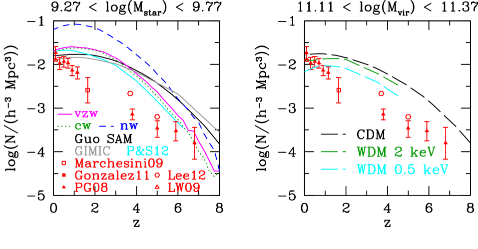
Figure 1: The evolution of the number density of galaxies with masses $\log(M_{\rm star}/M_{\odot})$=9.27-9.77 as a function of redshift. Red symbols with errorbars denote observational results. In the left panel, various model predictions are shown. Black lines denote results from the Guo et al. (2011) SAM, magenta solid lines are for the vzw model, blue dashed lines for the nw model, green dotted lines for the cw model, grey lines show results from GIMIC, cyan lines show results from Puchwein & Springel (2012). In the right hand panel, we compare observations to the number density evolution of haloes with masses $M_{\rm vir}=11.11-11.37$. Black dashed lines show results from the MS-II simulation, dark green and cyan dashed lines show results from two different WDM models, with a dark matter particle mass of 2 and 0.5 keV respectively.

More specifically, we show the number density evolution of galaxies in the stellar mass range 9.27 $<\log(M_{\rm star}/M_{\odot})<$ 9.77 versus redshift. Black and red data points on both panels show observational results from Pérez-González et al. (2008), Li & White (2009), Lee et al. (2012), González et al. (2011) and Marchesini et al. (2009). All observed stellar masses have been scaled to a Chabrier IMF. The offset at $z=0.1$ between Pérez-González et al. (2008) and Li & White (2009) is likely due to cosmic variance affecting the Pérez-González et al. estimate.

In the left panel, we compare observational results with predictions from various galaxy formation models. Black solid lines show results from the Guo et al. (2011) SAM. The solid magenta, dashed blue, green dotted, and grey lines show results from the vzw, nw, cw and GIMIC SPH simulations, respectively. On this plot alone, we also include results from a SPH simulation featuring a new ’energy-driven variable wind’ feedback scheme, recently suggested by Puchwein & Springel (2012). These results are shown as the cyan line. Clearly, there is a significant discrepancy between models and observations. For example, in the dataset of Pérez-González et al. (2008) the number of galaxies with $\log(M_{\rm star}/M_{\odot})=9.27-9.77$ increases by a factor of 2 from z=0.9 to z=0.1. In the SAM of Guo et al. (2011), it decreases by 7 % in the same redshift interval. The data point of Marchesini et al. (2009) at $z\sim 1.6$ is lower than any model by a factor of $\sim$ 5. More generally, the number of galaxies in the observations is roughly inversely proportional to redshift over the entire redshift range probed, while the models predict that the number density only increases steeply from high redshift to $z=1-2$, and then flattens. Turning to the SPH simulations, the GIMIC simulation resembles the SAM most closely, while the cw and vzw simulations show a steeper evolution, probably due to their lower mass resolution. The nw simulation, on the other hand, strongly overpredicts the number density of galaxies at $z=0$, which is not surprising given the absence of a strong feedback mechanism in this model. Finally, the simulation by Puchwein & Springel (2012) is slightly closer to observations at $z>0$, but a large discrepancy remains.

It is interesting to now consider the evolution of dark matter haloes that are likely to host the galaxies we consider here. In the right panel of Fig. 1, the black dashed lines show results for the evolution in the number density of dark matter haloes in MS-II, with $\log(M_{\rm vir}/M_{\odot})$ =11.11 - 11.37, which typically host the galaxies we consider at $z=0$ in the SAM. The resulting functional form is very similar to what has been found previously for dark matter-only simulations (Lukić et al. 2007). Clearly, the number density evolution of dark matter haloes of this mass is also very similar to that of the galaxies in the SAM (compare the black line in the left hand panel with the black dashed line in the right hand panel). This indicates that the relation between stellar mass and host halo mass barely evolves in the models: a galaxy with mass $\log(M_{\rm star}/M_{\odot})=9.27-9.77$ resides in a host halo with a very similar mass up to high redshifts (see also Sec. 7). If we compare the dark matter halo number density to the observational results, observations seem to require that the relation between stellar mass and halo mass evolves strongly in a $\Lambda$CDM cosmology. Haloes of fixed mass must host galaxies with lower stellar mass at higher redshift (as also found e.g. by Moster et al. 2010, 2012; Behroozi et al. 2010; Yang et al. 2011; Zehavi et al. 2012).

Given that it has been suggested that WDM might help to solve the problem, we also plot the number density evolution of haloes in this mass range in two WDM simulations with a dark matter particle mass of 2 keV and 0.5 keV. We find that while the normalisation changes slightly, the way the number density of haloes evolves is essentially unchanged with respect to CDM, indicating that the problem would likely also be present in a WDM Universe.

In summary, we confirm that the number density of low-mass galaxies evolves incorrectly in SAMs and verify that the problem also exists in SPH simulations. We suggest that, in both models, the growth of low-mass galaxies traces the growth of their host halos too closely, and that the mass of their host halos should increase to higher redshifts as also found in recent clustering and abundance matching studies (e.g. Yang et al. 2012).

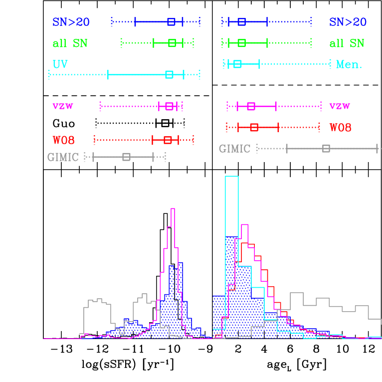
Figure 2: Model and observational results for specific star formation rates and luminosity-weighted stellar ages in the stellar mass bin $\log(M_{\rm star}/M_{\odot})=9.27-9.77$. Top panels show the median values (empty squares), the range within which 68 % of the values lie (solid errorbars) and the range within which 95 % of the values lie (dotted errorbars). Bottom panels show the full distributions for several selected datasets. The colour coding is as follows. Left panel: Blue and green: updated Brinchmann et al. (2004) sSFR, S/N$>$20 and the full sample. Cyan: UV sSFR from McGee et al. (2011). Magenta: vzw simulation. Black: Guo et al. SAM. Red: Wang et al. (2008) SAM. Grey: GIMIC simulation. Right panel: Blue and green: Gallazzi et al. (2005) luminosity-weighted ages for the $S/N>20$ and the full sample. Cyan: Mendel et al. sample. Magenta: vzw simulation. Red: Wang et al. (2008) SAM. Grey: GIMIC.

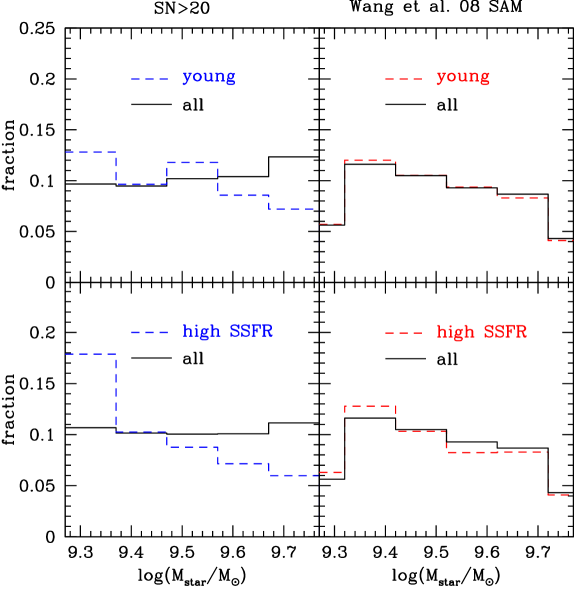
Figure 3: Stellar mass distributions in the observational sample and the W08 SAM in the stellar mass bin $\log(M_{\rm star}/M_{\odot})=9.27-9.77$. The black solid line is for the full sample, the coloured dashed lines are for the subpopulation of galaxies with ages below 2 Gyr (top panels) and $\log(\rm{sSFR})>$-9.5 (bottom panels). Clearly, the strongly star forming and young galaxies tend to have low masses in the observations, while there is nearly no such trend in the models. The full sample is slightly different in the top and bottom left panel, since age estimates are not available for all galaxies.

4 Approach I – Low mass galaxy properties

We proceed to compare specific star formation rates and stellar ages for galaxies with masses $\log(M_{\rm star}/M_{\odot})$=9.27-9.77 in the observations and models. We only focus on central galaxies, since satellite galaxies are not correctly reproduced in current models (e.g. Weinmann et al. 2011b).

While in the observations and in the models of Davé et al. (2011), satellites seem to be a subdominant population at these stellar masses, this is not the case for the semi-analytic models. The Guo et al. (2011) SAM predicts that as many as 50 % of the galaxies at $z$=0 in the stellar mass range we consider are satellites.

We do not include the constant-wind and no-wind simulations by Davé et al. (2011a, b) in the following comparisons, since the constant-wind simulation is similar to GIMIC, and the no-wind simulation is very far off the observations at $z$=0.

4.1 Low redshift results

4.1.1 Specific star formation rate

In Fig. 2, left panels, we show the distribution of specific star formation rates in our various datasets, including models and observations. The top left panel shows the median sSFR as an empty square, the range within which 68 % of galaxy sSFR lie as solid errorbars, and the range encompassing 95 % of the sSFR as dotted errorbar. The bottom panel shows the full distribution for several selected subsets. Model galaxies with a SFR of zero are assigned a random value between log(sSFR)=-11.6 and -12.4. The sSFR from UV and from the updated Brinchmann et al. (2004) method are in good agreement, except for an extended tail of low sSFR galaxies in the UV, which corresponds to the UV non-detections.

The agreement between the median log(sSFR/yr) in the observations ($\sim-9.95$ ) and the vzw model ($\sim-10.0$) is surprisingly good, given the large discrepancy between observed and model sSFR at low masses found by Davé et al. (2011a). The reason for this difference appears to be that Davé et al. (2011) used observations by Salim et al. (2007) that were restricted to a star-forming sample of galaxies to compare to their model galaxies. The median log(sSFR/yr) in the Guo et al. (2011) model is slightly lower ($\sim-10.1$), but also in relatively good agreement with observations, in contrast to the substantial offset found in previous work (Fontanot et al. 2009; Guo et al. 2011). This difference, in turn, is due to the exclusion of satellite galaxies in our comparison, whose properties are likely incorrect in SAMs.

Crucially however, the models seem to miss a tail of high star formation rates that are present in the observations. While 9 % of galaxies in the S/N$>$ 20 sample have $\log$(sSFR)$>-9.5$, this is only the case for 1.5 % of galaxies in the Guo et al. (2011) model, and for 0.4 % of galaxies in the vzw model. We note that if these galaxies have formed stars at the current rate or higher in the past, they have formed entirely in less than 3 Gyr, i.e. since $z$=0.3. About 2.5 % of galaxies even have log(sSFR) in excess of -9.2, meaning they could have formed all their stars within the last 1.6 Gyr, or since z=0.15. The fact that we find such highly star forming galaxies independent of whether the UV sSFR or the Brinchmann et al. (2004) sSFR is used indicates that the discrepancy with models is robust. We have checked that a similar picture is seen at $z=1$ in the ROLES data by Gilbank et al. (2011) who use the O[II] line to estimate star formation. At $z=1$, $\sim$ 15 % of galaxies have doubling times of less than 1 Gyr in the observations, while this is the case for less than 2 % in the Guo et al. (2011) model.

At the other end of the distribution, we find 14 % of galaxies in the S/N$>$20 sample with $\log$(sSFR)$<$-11. Only 6 % of galaxies in the Guo et al. sample have such low star formation rates, and less than 4 % in the vzw sample. This difference could be due to (i) contamination of the observed sample by satellite galaxies or (ii) a real quiescent population of central galaxies that is more abundant than in the model. (i) seems an unlikely explanation, as the contamination of the central sample by satellites is estimated to be only around 3 % (Weinmann et al. 2009). Our result might thus be in tentative agreement with the population of red, isolated, faint central galaxies in the SDSS that seems to have no counterpart in semi-analytic models (Wang et al. 2009).

We note that the GIMIC simulation strongly underpredicts star formation rates. While this might partially be because star-formation rates are not resolution-converged in GIMIC, the discrepancy we find seems in line with the usual problems of standard hydrodynamical simulations (e.g. Avila-Reese et al. 2011). In general, galaxies in those simulations form in an early strong burst of star formation (Scannapieco et al. 2012), leading to strong feedback that makes the galaxies almost passive by the present day (see Section 5.4). Since GIMIC does reproduce the evolution of the cosmic star formation rate density, star formation in this simulation is overly concentrated in massive galaxies at low redshift (see Fig. 5 of Crain et al. 2009).

As mentioned before, the good agreement between observations and the semi-analytical model is due to the exclusion of satellites. If we include satellites, the median sSFR of SDSS galaxies only decreases slightly compared to the full sample, to log(sSFR)=-10.05. The median sSFR of galaxies in the Guo et al. sample, however, goes down to log(sSFR)=-10.43. Also, the passive fraction (with log(sSFR) $<$ -11) in the observations increases only to 24 %, while it reaches 42 % in the Guo et al. model. Including satellites has a much more moderate effect in the vzw simulation; it changes the median to log(sSFR)=-10.04, in excellent agreement with observations, and increases the fraction of passive galaxies only to 14 %, which is still lower than the passive fraction of the full observed sample, indicating that the satellites in the vzw model are in fact quenched too little.

We conclude that there seems to be insufficient diversity in the star formation rates of model galaxies. Part of the reason for this could be that star formation in the models is not sufficiently bursty. Also, the median sSFR is slightly too low in models. Both of these problems may be related to the weak evolution in the number density of model galaxies at late times.

4.1.2 Luminosity-weighted Stellar Ages

In Fig. 2, right panels, we show luminosity-weighted ages from Gallazzi et al. (2005, blue lines), and from Mendel et al. (cyan lines). They are compared to $r$-band luminosity weighted ages from the vzw-model (magenta lines) and $V$-band luminosity-weighted ages from Wang et al. (red lines). We convolve all model results with a Gaussian distribution with $\sigma$=0.15 in logarithmic age which is the mean 68 % confidence range as indicated in Gallazzi et al. (2005) for our stellar mass bin.

Model and observed distributions are clearly different. In the $S/N>20$ sample of Gallazzi et al. (2005), more than 40 % of galaxies have ages below 2 Gyr, while this is the case for only 16 % in the Wang et al. (2008) sample. The luminosity-weighted ages of Mendel et al. and of Gallazzi et al. (2005) are in good agreement, despite being based on two different SSP models (Maraston 2005 vs. Bruzual & Charlot 2003). This indicates that the observational result is robust.

These results indicate that the models not only lack the subpopulation of galaxies currently having high star formation rates (see Section 4.1.1), but also predict too little star formation in the last 2-3 Gyr. We have checked that while sSFR and age are broadly anti-correlated in the observations as expected, many of the galaxies with young ages do not have particularly high current sSFR. A similar problem, but regarding ages weighted according to stellar mass and not according to luminosity (which are more uncertain, see Gallazzi et al. 2008) has been found by Somerville et al. (2008), Fontanot et al. (2009) and Pasquali et al. (2010).

4.1.3 What are the young and star forming galaxies?

We have pointed out that the fraction of young (ages below 2 Gyr) and very active (log(sSFR)$>$-9.5) galaxies is higher in the observations than in the models. In Fig. 3 we show the distribution in stellar mass for the young and active galaxies compared to the full sample both for the $S/N>20$ observations, and for the Wang et al. (2008) model. We use a binning of 0.1 dex, which is half the expected error in stellar mass according to Gallazzi et al. (2005). Using a larger binning does not change the basic trends that these figures show: In the observations, lower mass galaxies are on average younger and have higher sSFR. This indicates that it is especially the galaxies just entering our stellar mass bin which are too passive and too old in the model. From this it follows that the rate of galaxies entering the mass bin is probably too low, which may explain the missing evolution in the number density we found in Fig. 1.

5 Approach II – Toy model

In our second approach to understanding the number density evolution of low mass galaxies, we employ a simple toy model to check if the observed evolution of the stellar mass function and the sSFR-stellar mass relation can be reconciled. We find that this is the case if we adopt a relatively shallow slope in the sSFR-stellar mass relation, as found by several observational studies.

We start with the analytical fit to the stellar mass function at $z$=0.9, as obtained by Pérez-González et al. (2009), cut off at $M_{\rm star}=10^{7}M_{\odot}$. This stellar mass function is then evolved up to the present day, assuming that all galaxies follow the same relation sSFR($M_{\rm star},z$) and that 40 % of newly formed stars are immediately returned to the ISM, according to a Chabrier IMF. The final stellar mass function is then compared with the $z$=0 stellar mass function obtained by Li & White (2009) (including the correction by Guo et al. 2010). Both the Pérez-González et al. (2009) and Li & White (2009) MF have been scaled to a Chabrier IMF.

Our toy model is based on the fact that the evolution of the mass function can be described by a simple continuity equation, as explained in more detail in Drory & Alvarez (2008). As an input to this continuity equation, we need the average relation between sSFR and stellar mass for the full population of galaxies. The scatter around that relation, and the fraction of passive galaxies, however, do not need to be known. Similar approaches have been used by Bell et al. (2007), and by Peng et al. (2010). Like these models, our toy model requires extrapolation of the stellar mass function and the sSFR-stellar mass relation below the observational limits.

5.1 The observed sSFR-stellar mass relation

Following Karim et al. (2011), we parameterize the relation between star formation, redshift and mass as:

$$\log({\rm sSFR(M_{\rm stellar},z)})=C+\beta\log(M_{\rm stellar})+\alpha\log(1+z).$$ (2)

$\alpha$ is usually found to be about 3-4.5 (e.g. Damen et al. 2009; Karim et al. 2011; Fumagalli et al. 2012). $\beta$, on the other hand, that parameterizes the correlation between sSFR and stellar mass, is usually found to be negative in observational studies up to at least $z\sim 2$. Karim et al. (2011), for example, find $\beta\sim$ -0.4 and $\beta\sim$ -0.7 for their full/star-forming samples respectively, Drory & Alvarez (2008), including an incompleteness correction for galaxies with low SFR, find $\beta$ between -0.3 and -0.4, Noeske et al. (2007) find $\beta\sim$ -0.3 for star-forming galaxies, and Whitaker et al. (2012) find $\beta\sim$ -0.4 for their full sample. A less steep slope is advocated by Salim et al. (2007; $\beta$=-0.17 for low mass star forming galaxies). Elbaz et al. (2007), Daddi et al. (2007) and Dunne et al. (2009) all find $\beta$=-0.1, with the former two samples being restricted to star-forming galaxies, and the latter referring to a $K$-band selected sample.

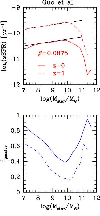
Figure 4: Mean sSFR (top panel, in red) and passive fractions (with log(sSFR)$<-11$, bottom panel, in blue) in the Guo et al. (2011) SAM at $z=0$ (solid lines) and $=1$ (dashed lines) as a function of stellar mass. The average relation between sSFR and mass in the SAM is almost perfectly fit by a positive slope of $\beta$=0.0875, while the evolution in redshift is fit by a factor of $(1+z)^{2.15}$ (black lines). This is very close to the corresponding relations for dark matter haloes (Neistein & Dekel 2008), but at odds with observational results.

5.2 The sSFR-stellar mass relation in models

We check the same relation in the Guo et al. (2011) SAM in Fig. 4, top panel, where we show the mean relation between log(sSFR) and $\log(M_{\rm star})$ at $z=0$ and $z=1$ in the SAM (including satellite and central galaxies), to which we fit a linear relation. We find that $\beta$=0.0875 and $\alpha$=2.15 provides a good fit at $\log(M_{\rm star}/M_{\odot})$=7-11 both at $z=0$ and $z=1$. If we exclude satellite galaxies, $\alpha$ and $\beta$ remain virtually unchanged (only the normalization of the sSFR shifts up). Remarkably, both $\alpha$ and $\beta$ as found in the Guo et al. (2011) SAM closely resemble the scaling expected for the specific dark matter accretion rate, where $\beta\sim 0.1$ and $\alpha\sim 2.2$ (Neistein & Dekel 2008). This similarity between sSFR and specific dark matter accretion rate is interesting given the presence of strong feedback in the SAM; in hydrodynamical simulations, the baryonic accretion rate already deviates from this scaling (Faucher-Giguère et al. 2012).

In the lower panel of the same Figure, we show the passive fraction of galaxies as a function of stellar mass in the SAM for illustration. Clearly, the passive fraction strongly increases towards lower stellar mass, and this is what is causing the positive correlation between stellar mass and sSFR. If we remove all passive galaxies in the SAM, we find $\beta\sim 0$ at $z=1$ and $\beta\sim-0.1$ at $z=0$. This means that the positive slope in the SAM comes from an overprediction of the number of passive galaxies in the model.

We note that sSFR and stellar mass are even more strongly positively correlated in the vzw model, where $\beta\sim 0.25$ at $\log(M_{\rm star}/M_{\odot})=9-10$ (see Davé et al. 2011).

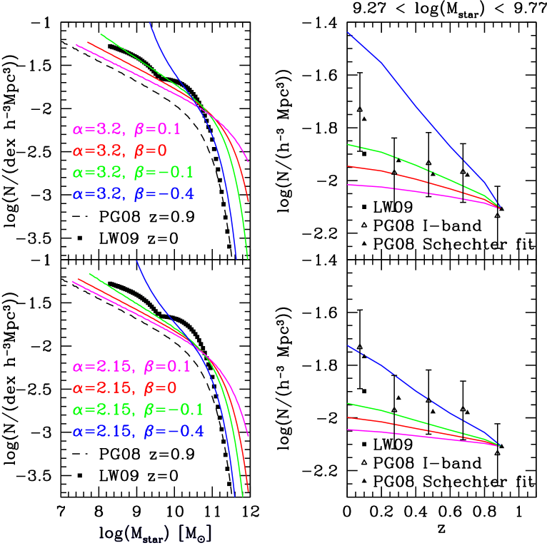
Figure 5: A toy model showing the evolution of the stellar mass function starting from the $z=0.9$ mass function by Pérez-González et al. (2008) (dashed line in the left panels) and assuming all galaxies follow the same sSFR($z$, $M_{\rm star}$) with varying $\alpha$ and $\beta$, where $\alpha$ expresses the dependence of the sSFR on (1+$z$), while $\beta$ denotes the slope in the sSFR-stellar mass relation. Top panels are for $\alpha=3.2$, bottom panels for $\alpha=2.15$. In the left panels, we compare the toy model results to the observed evolution of the stellar mass function. Solid black squares show the stellar mass function from Li & White (2009) at $z=0$. In the right panels, we show a plot similar to Fig. 1, truncated at $z=1$. As we need to use the analytical stellar mass function at $z=0.9$, we also show the number density obtained from integrating the analytical Schechter form of the stellar mass function as obtained by Pérez-González et al. (2008) (points without error bars). They are notably offset from the directly measured number densities, which indicates that the Schechter fit is not perfect at the masses we consider.

5.3 Results of the toy models

In Fig. 5, we show 8 simple models with varying $\alpha$ and $\beta$, and compare them with both the stellar mass function evolution (left panels) and the evolution in the number densities (right panels) since $z=0.9$. In the top panels, we use $\alpha$=3.2, following observational results of Fumagalli et al. (2012), in the bottom panels we use $\alpha$=2.15, following the SAM. We vary $\beta$ between 0.1, 0, -0.1 and -0.4, and fix $C$ such that log(sSFR)=-9.95 at $\log(M_{\rm star}/M_{\odot})$=9.52, as we find in the SDSS. The results show that that the amount of evolution in the stellar mass function between $z=1$ and $z=0$ depends very strongly on $\beta$, and less on $\alpha$. We do not include any parameterization for mass quenching or mergers in our simple model (see Peng et al. 2010 for a way in which this may be done). For this reason, most of our models overproduce the high mass end of the mass function at $z=0$ (which is however subject to some uncertainties, see Bernardi et al. 2010).

The best agreement with the observed evolution of the low-mass end of the stellar mass function is found for $\beta\sim-0.1$, i.e. a modest negative correlation between sSFR and stellar mass. If $\beta\sim$ 0.1, as found in the SAM, the evolution in the stellar mass function is weak, resembling the weak evolution found in the stellar mass function by Guo et al. (2011) and evidenced in our Figure 1. Thus the missing evolution in the stellar mass function in the SAM is likely due to a positive correlation between sSFR and stellar mass. Models thus need to find a way to break the close link between specific star formation rates and specific dark matter accretion rates.

A negative correlation between sSFR and stellar mass is a form of ’downsizing’ (Cowie et al. 1996). At late times, lower mass galaxies are observed to form stars more vigorously relative to their stellar mass than higher mass galaxies. In contrast, lower mass haloes are predicted to grow more slowly relative to their mass in a CDM cosmology. It appears that this form of downsizing, if real, is still not explained by current models.

Fig. 5 also shows that $\beta=-0.4$, as found e.g. by Karim et al. (2011), cannot hold down to low masses, as it would lead to a too rapid evolution in the stellar mass function. A similar conclusion was reached by Drory & Alvarez (2008), who speculate that either (i) the excess growth at the low mass end due to star formation needs to be removed by mergers or (ii) the observational finding that $\beta\sim-0.4$ is incorrect and due to surveys missing passive low mass galaxies. Also, in agreement with our results, Conroy & Wechsler (2009) find that observations of mass growth and star formation at $z<1$ are roughly self-consistent, using $\beta\sim-0.2$.

We thus conclude that the problem in the number density evolution in the models is caused by a positive, instead of a negative correlation between sSFR and stellar mass in the models (see Fig. 4). We also find that the observed evolution of the low mass end of the mass function is consistent with the sSFR-stellar mass relation as observed by Dunne et al. (2009), Daddi et al. (2007) and Elbaz et al. (2007), who find $\beta\sim$-0.1.

5.4 The star formation histories

To establish the link between the toy model, and the models discussed in the first part of the paper, it is instructive to consider the star formation histories (hereafter SFH) of galaxies. We define the SFH here as the star formation rate of all resolved progenitor galaxies together, divided by the total stellar mass ever formed. In the left panel of Fig. 6, we show the SFH of central galaxies with 9.27 $<\log(M_{\rm star}/M_{\odot})<$9.77 in the Guo et al. SAM, GIMIC and in the vzw model.

Reflecting the severe differences between GIMIC on the one hand and the vzw and SAM on the other hand seen in Section 4, the SFH of galaxies in GIMIC is markedly different from the other models. GIMIC predicts a strong initial peak, followed by a decline, similar as seen in other hydrodynamical models (e.g. Scannapieco et al. 2012). The vzw simulation, on the other hand, predicts a SFH that is nearly constant with time in this stellar mass bin, while the SAM shows a mildly decreasing SFH.

At first sight, it may seem surprising that such a different SFH as in GIMIC and in the vzw simulation results in such a similar number density evolution of galaxies at fixed stellar mass, as seen in Fig. 1. These results can however be reconciled if one considers that the two figures refer to different galaxies at $z>0$, and if one takes into account the evolution of the stellar-to-halo mass ratio, as we explain in sec 7.

Of course, to understand the evolution of number densities in Fig. 1, and to compare the GIMIC, vzw model and the SAM to the toy model, we need to consider the average SFH of all galaxies in those models, and not only the central galaxies. In the middle panel, we therefore show the SFH of the Guo et al. (2011) SAM galaxies for all, centrals, and satellites separately. Clearly, satellites have a different SFH than centrals, lowering the overall SFH at late times.

In the right panel, we again overplot results for all galaxies from the SAM and compare it to the SFH given by our toy model for the same stellar mass bin for $\alpha$=2.15 and $\alpha$=3.2, and $\beta$=-0.1 and $\beta$=0.1. Recall that $\beta$=-0.1 roughly reproduces the observed evolution of the mass function, while $\beta$=0.1 is very similar to the value in the SAM and leads to too little evolution. The toy models do not have a SFH before $z$=0.9 by construction. Interestingly, the difference between SFH of models that reproduce the number density evolution ($\beta$=-0.1), and those that do not ($\beta$=0.1), is very mild. Only a slight boost in the SFH, mostly at $z\sim 0.5-1$, is enough to overcome the problem that we have seen in the number density evolution. The small difference in the SFH might give the impression that the problem in the SAM and the hydrodynamical models should be easy to solve. This is not necessarily the case. Boosting the sSFR by a small amount may be difficult, as the necessary gas reservoir has to be in place, neither having been ejected, stripped (in the case of satellite galaxies) nor having been converted into stars. We note that results for the SFH in our toy model seem to be in reasonable agreement with the SFH derived by Leitner (2012) using main sequence integration.

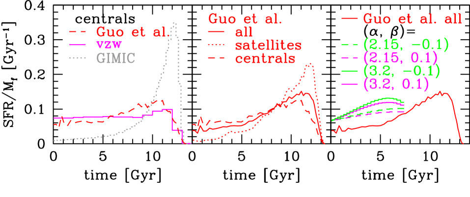
Figure 6: Star formation histories of galaxies from various models in the stellar mass bin 9.27 $<\log(M_{\rm star}/M_{\odot})<$ 9.77, normalized by the total stellar mass ever formed in those galaxies. Left panel: SFH of central galaxies from the Guo et al. SAM (red dashed line), the vzw-simulation (magenta solid line) and the GIMIC simulation (grey dotted line). Middle panel: SFH for all, satellites and centrals in the SAM shown separately. Right panel: SFH from toy models with $\alpha$ varying between 2.15 and 3.2, and $\beta$ varying between -0.1 and 0.1, for all galaxies. Models with $\beta$=0.1 predict insufficient evolution in the MF between $z=1$ and $z=0$, while models with $\beta$=-0.1 produce sufficient evolution. Yet, the difference in their SFH is not dramatic.

6 Discussion

6.1 Two open problems in low mass galaxy evolution

We find two open problems in low mass galaxy evolution. First, we confirm a serious discrepancy in the evolution of the number density of galaxies at fixed stellar mass in semi-analytic and SPH models.

Second, we show that models do not reproduce the population of low mass galaxies with high sSFR and young ages at $z<1$. The problem becomes more severe towards lower stellar masses. Put differently, as shown in Section 5, models do not reproduce the observed negative slope in the sSFR-stellar mass relation (see e.g. Somerville et al. 2008). Instead, the slope is positive, which may directly cause the too slow evolution in the number density of low mass galaxies. The two problems are thus likely closely connected.

6.2 Potential explanations by observational issues

The offset between observations and models at $z>0.5$ could also stem from an incorrect interpretation of the observations. The two main potential explanations are (i) the IMF is variable, leading to problems in the estimates of mass and SFR and (ii) observations are missing more galaxies than expected.

Option (i) is difficult to prove wrong. The observed high sSFR at $z\sim 1-2$ that are hard to reproduce by models seem to favour a bottom-light IMF (e.g. Davé 2008). If one assumes such a bottom-light IMF, however, this decreases the observed high redshift mass function even more (see Marchesini et al. 2009), making the discrepancy with models worse. More complex solutions are impossible to rule out completely and need to be tested with self-consistent models, as a varying IMF will also affect other processes like feedback.

Option (ii) cannot be completely ruled out either, but there are several arguments against it. Up to now, no indication of a large and unexpectedly faint population of low mass galaxies has been found despite the varying depth of different surveys. Nevertheless, it is possible that all surveys have missed a population of very passive and/or dusty low mass galaxies $z>0$. One argument against this is that such galaxies are not seen in large numbers in the models either. For example, in Guo et al. (2011), the fraction of passive galaxies at $z=1$ is only 20 % in the mass bin we consider (see Fig. 4, bottom panel.) Also, observations do not find a large population of passive low mass galaxies at $z$=0 (e.g. Geha et al. 2012). Even in the local volume, where selection effects are minimal, a tight star formation sequence for low mass galaxies has been found (Lee et al. 2007). It is thus hard to imagine that passive low-mass galaxies would be more numerous at higher redshifts, where the global star formation rate density is higher. Finally, we note that the problem in the number density evolution persists up to a mass of $\log(M_{\rm star}/M_{\odot})\sim$ 10.5 (see e.g. Guo et al. 2011), where missing a large number of galaxies becomes more unlikely. But also if we assume that observations missing a large number of passive galaxies is the solution to the problem, this would mean that star formation does behave very differently than assumed in current models, possibly cycling between bursty and passive episodes. This would still constitute a rather fundamental problem for current galaxy formation theory and would probably require more efficient high $z$ feedback as well (see below).

6.3 Potential implications

If the problem with models at $z<1$ is real, which seems likely, a process suppressing galaxy formation at high redshift is needed, so that the build-up of the mass function below $M^{*}$ can happen at a far later time than the predicted build-up of the dark matter haloes in which they reside (see also Conroy & Wechsler 2009). Such a process would perhaps also address the problem of the overproduction of satellite galaxies in models (Weinmann et al. 2006, Lu et al. 2012), as those form early.

Several mechanisms have been suggested, but all of them seem to have some drawbacks. Decreasing the star formation efficiency at high redshift leads to an overproduction of cold gas in low mass galaxies (e.g. Wang et al. 2012). Preheating the IGM (Mo et al. 2005) does not seem possible with known mechanisms (Crain et al. 2007). Warm dark matter also does not seem a viable solution, as we have shown in Section 3. More exotic dark matter candidates like ultra-light dark matter (Marsh et al. 2010) or mixed dark matter (Boyarski et al. 2009) may need to be considered, but the problem remains that observations of the Lyman-alpha forest require substantial power on small scales (Seljak et al. 2006).

Thus, perhaps the most natural change to galaxy formation models is changing the stellar feedback prescription. In most current models, the efficiency with which gas is ejected from the cold gas reservoir scales roughly as

$$\dot{M}_{\rm wind}/\dot{M}_{*}\propto V_{\rm vir}^{-\gamma}\propto M_{\rm vir}^{-\gamma/3}t_{\rm H}^{\gamma/3},$$ (3)

with $M_{\rm vir}$ the halo mass and $t_{\rm H}$ the Hubble time. Semi-analytic models use $\gamma\sim 2-6$ (Croton et al. 2006, Bower et al. 2006, Somerville et al. 2008, Guo et al. 2011). In most current hydrodynamical models like GIMIC, the initial velocity and mass-loading of the wind is independent of the host halo mass, i.e. $\gamma=0$. However, Neistein et al. (2012) show that effectively, $\gamma\sim 3/2$ in such simulations, due to gravitational and hydrodynamical interactions. In the momentum-driven winds (vzw) model by Oppenheimer & Davé (2008), the winds are launched with $\gamma$=1 (with the velocity dispersion replacing $V_{\rm vir}$). The effective $\gamma$ is thus likely higher than 3/2. The recently proposed wind scheme by Puchwein & Springel (2012) that we included in Fig. 1 launches winds with $\gamma\sim 2$.

As $\gamma>0$ in all these models, this means that their star-formation driven feedback at a given halo mass is less efficient at earlier times. As long as the feedback follows this basic scaling, and as long as star formation and cooling become more efficient towards higher redshift, it is no surprise that no model is able to predict the steep decrease in the stellar-to-halo mass ratio towards higher redshifts, which seems demanded by observations (see our Fig. 1, Moster et al. 2010, 2012; Yang et al. 2011). The same problem likely also causes the inability of the models to reproduce the negative correlation between sSFR and stellar mass. In fact, the few models that we are aware of which reproduce the correlation (the nw model in Davé et al. 2011, and the no-feedback model in Neistein & Weinmann 2010) have little or no feedback. This means that increasing the star-formation driven feedback efficiency arbitrarily will probably never solve the basic problem. What may be needed, therefore, is a justification to use a different functional form for feedback.

One potential solution might be a more top-heavy IMF at high redshift, which could produce more massive stars that are short-lived and drive highly mass-loaded winds. For example, the contribution of winds from O and B stars depends strongly on the upper mass cutoff of the IMF (Leitherer et al. 1992), but of course, a change in the IMF would also affect stellar mass and star formation rate estimates. Alternatively, highly concentrated, clumpy star-forming regions could also cause higher feedback efficiencies (Guedes et al. 2011; Brook et al. 2012).

Another potentially important mechanism for understanding the evolution of the number density of galaxies is ’reincorporation’ or ’GSW recycling’ of material ejected from the galaxy (Oppenheimer et al. 2010). In semi-analytic models, reincorporation is often assumed to scale either with $t_{\rm H}^{-1}$ (Croton et al. 2006), or with $M_{\rm vir}^{-1/3}\times t_{\rm H}^{-4/3}$ (Guo et al. 2011). In both cases, it is thus most important at early times. This means that the net efficiency of outflow of mass from a given host halo, which is the outflow efficiency minus the reincorporation efficiency, is low at high redshift in these models for two reasons: First, the feedback efficiency is low, and second, the reincorporation efficiency is high. At late times, when it could boost star formation rates, it is least efficient. This basic scaling used in semi-analytic models thus works against solving the problem. Also, it is not confirmed by SPH simulations: Oppenheimer et al. (2010) have found a much weaker dependence on time, which makes recycling relatively more important at late times, and probably explains why the vzw model produces an almost constant SFH at $\log(M_{\rm star}/M_{\odot})\sim 9.5$. On the other hand, GSW recycling is more efficient for high mass haloes than for low mass haloes, which exacerbates the problem of the incorrect relation between sSFR and stellar mass (Firmani, Avila-Reese & Rodríguez-Puebla 2010).

6.4 Reconciling the star formation histories and number density evolution

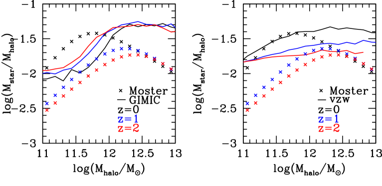
Figure 7: The stellar-to-halo mass ratio as a function of halo mass. Crosses show abundance matching results from Moster et al. (2012). On the left, results from GIMIC are overplotted, on the right, from vzw. $z=0$ results are shown in black, $z=1$ results in blue and $z=2$ results in red.

One interesting result of our study is that the number density evolution of low mass galaxies is very similar in all models (Fig. 1), although the star formation rates, ages (Fig. 2) and star formation histories (Fig. 6) of the galaxies which populate the mass bin at $z=0$ are very different.

To link these results, it is instructive to consider the stellar-to-halo mass ratio of galaxies as a function of halo mass. We show this quantity as calculated by Moster et al. (2012) from abundance matching, compared to central galaxies in GIMIC and vzw, in Fig. 7, with colours denoting $z=0$ (black), $z=1$ (blue) and $z=2$ (red).

Two interesting points can be noted from this figure. First, the stellar-to-halo mass ratio of haloes with mass $\log(M_{\rm halo}/M_{\odot})\sim 11.25$, which host the galaxies in our stellar mass bin at $z=0$, evolves very little up to $z=2$ both in the vzw and GIMIC simulations. This explains the fact that the number density evolution is fairly similar in those models in Fig. 1. Observations, on the other hand, seem to demand a much stronger evolution in the stellar-to-halo mass ratio since $z=1$ at these halo masses.

Fig. 7 also helps us to understand the large differences in the SFH between GIMIC, vzw and what we have derived from our toy model in Fig. 6. Assume that in all cases we start with a halo of mass $\log(M_{\rm halo}/M_{\odot})$ = 11.1 at $z=1$, growing to 11.3 at $z=0$. In GIMIC, the mass of the central galaxy will only grow by 20 %, since the stellar-to-halo mass ratio actually decreases from $z=1$ to $z=0$, thus requiring only very little star formation. In vzw, on the other hand, the central galaxy needs to grow by a factor of 2.5 in the same period, in good agreement with the much higher late SFR in this model. Looking at the Moster et al. (2012) results, the same galaxy needs to grow by a factor of about 8, obviously requiring even more late star formation, well in line with the results from our toy model in Fig. 6.

7 Conclusions

We have investigated the dramatic failure of models to predict the number density evolution of galaxies with stellar masses of about $\log(M_{\rm star}/M_{\odot})$ $\sim$ 9.5. For this, we have used two approaches. First, we have compared the $z=0$ properties of low mass galaxies in models and observations, using two different semi-analytic models and two different hydrodynamical simulations, and excluding satellite galaxies. Second, we have built a simple toy model to investigate the link between the sSFR as a function of redshift and stellar mass, and the evolution of the mass function.

Our main findings are as follows.

• We confirm the potentially serious problem in the number density evolution of galaxies with $\log(M_{\rm star}/M_{\odot})$ $\sim$ 9.5. The observed evolution in the number of galaxies at fixed stellar mass is much steeper than in the models. This indicates that the growth of galaxies at high redshift is too efficient in the models, causing galaxies to be in place too early. We show that this problem does not only appear in SAMs, but also, in remarkably similar form, in SPH simulations, indicating that it is a real problem in the current theory of galaxy evolution. We also show that the number density evolution of model galaxies closely matches that of dark matter haloes hosting these galaxies at $z=0$. Such a close correspondence between galaxies and dark matter haloes seems to be missing in the real Universe, if we assume a $\Lambda$CDM cosmology. We have also found that assuming a WDM instead of CDM cosmology gives a very similar number density evolution of dark matter haloes, which indicates that WDM will likely not help to solve the problem we describe in this work.

• This problem in the number density evolution is likely related to the fact that the models fail to reproduce the 40 % of central galaxies with luminosity-weighted ages below 2 Gyr, and the 10 % with star formation rates in excess of log(sSFR)=-9.5 at $z=0$ in our stellar mass bin. We find that a similar problem appears at $z=1$, and that the problem seems to become more severe towards lower stellar masses. It seems that many low mass galaxies have experienced substantial recent growth, which is a phenomenon not seen in models.

• In order to understand the potential link between the evolution of number densities and the sSFR-stellar mass relation, we build a simple toy model. We find that the evolution of the stellar mass function with time is very sensitive to the assumed slope in the sSFR-stellar mass relation, $\beta$, with sSFR $\propto M_{\rm star}^{\beta}$. In models, $\beta$ is usually positive, causing a very slow evolution of the low-mass end of the stellar mass function. The relatively fast observed evolution of the stellar mass function, on the other hand, favours a negative beta, with $\beta\sim-0.1$. This means that the observations advocating $\beta\sim-0.1$ seem consistent with the observed evolution of the mass function. We point out that $\beta\sim-0.4$, as found by some observational studies directly measuring the sSFR, would cause a too strong evolution in the mass function, confirming results by Drory & Alvarez (2008).

• The inability of the models to reproduce the number density evolution of galaxies, the population of young and star forming galaxies and the negative correlation between sSFR and stellar mass seem all to be part of the same underlying problem: Despite the presence of strong stellar feedback, model galaxies closely follow the evolution of dark matter haloes in a $\Lambda$CDM cosmology. As low mass dark matter haloes form earliest and evolve the least in a hierarchical cosmology, low mass galaxies also come out old and evolved today, in clear contrast with observational results. It is thus necessary to find a way to decouple the halo accretion rate and the star formation rate of low mass galaxies.

  Finally, the failure of all models to suppress galaxy formation at high redshift is likely caused by the fact that most feedback prescriptions are essentially of the same flavor in these models. The feedback efficiency in most current models scales as $M_{\rm vir}^{-\gamma/3}t_{H}^{\gamma/3}$ where $\gamma\geq 0$, resulting in a reduced feedback efficiency for a given halo mass at earlier time. The overproduction of low-mass galaxies at $z>0.5$ in all SAMs and hydrodynamical simulations explored here may thus be symptomatic of the limited range of feedback prescriptions currently in use, and indicates that alternative models of feedback need to be explored. Other potential remedies include metallicity-dependent star formation laws, an evolving IMF, observations missing an unexpectedly large number of galaxies at high redshift, or perhaps some form of pre-heating.

Appendix A Additional comparisons

Below, we compare the dust attenuations and stellar metallicities between models and observations in our stellar mass bin at $z=0$. We find that agreement is reasonable, except that SAMs underpredict the dust attenuation in galaxies.

A.1 Stellar metallicities

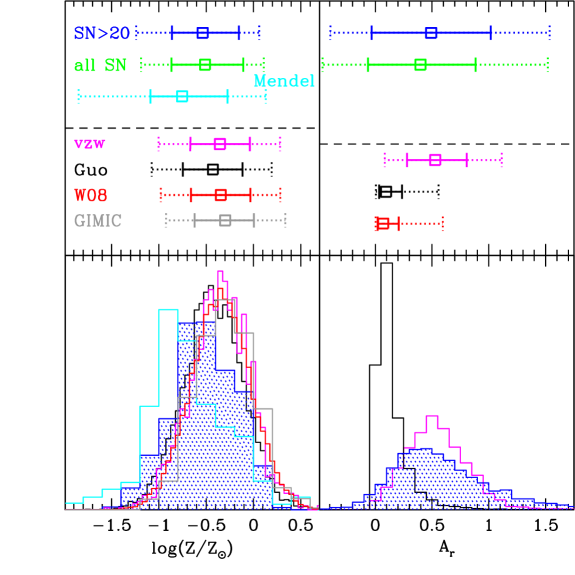
Figure 8: Model and observational results for the stellar metallicities (left panels) and dust attenuations (right panels) in the stellar mass bin $\log(M_{\rm star}/M_{\odot})=9.27-9.77$. Top panels show the median value (empty square), the range within which 68 % of the values lie (solid errorbars) and the range within which 95 % of the values lie (dotted errorbars). Bottom panels show the full distributions for some selected datasets. The colour coding in the left panel is as follows. Blue and green: Gallazzi et al. (2005) luminosity-weighted metallicities for the $S/N>20$ and the full sample. Cyan: Mendel et al. sample. Magenta: vzw simulation. Red: Wang et al. (2008) SAM. Grey: GIMIC. Blue and green: dust attenuation following Kauffmann et al. (2003), S/N$>$20 and the full sample. Magenta: vzw simulation. Black: Guo et al. SAM. Red: Wang et al. (2008).

In Fig. 8, left panels, we show the distribution of stellar metallicities for our various samples. The metallicities are luminosity-weighted for the observed sample [blue and cyan lines for the Gallazzi et al. (2005) and Mendel et al. estimates, respectively] but stellar mass-weighted for all the models. For the SAMs and GIMIC, total metallicities are a direct model output, while they are calculated from the Fe and O abundance for the vzw model, and computed from spectral indices in the observational data.

We convolve all model results with a Gaussian distribution with $\sigma$=0.3 in log($Z$) which is the mean 68 % confidence range as indicated in Gallazzi et al. (2005) for the corresponding stellar mass bin. Interestingly, metallicities from the Wang et al. (2008) model, the Guo et al. (2011) model and the vzw simulation are in near perfect agreement with each other, indicating that the predictions of models are robust in this respect. They are also in reasonable agreement with observations. The remaining relatively small offset between models and observations could be due to the difference between mass-weighted and luminosity-weighted metallicities. Davé et al. (2011b) obtain qualitatively similar results when comparing gas-phase metallicities in the vzw simulation to observational results.

A.2 Dust

In Fig. 8, right panel, we show the distribution of $r$-band dust attenuation in models and observations. Both semi-analytic models seem to include too little dust attenuation. On the other hand, the vzw model predicts dust attenuations in good agreement with the SDSS estimates. This is not surprising as dust attenuation in this model is included following the observed relation between metallicity and dust attenuation. It is interesting that the Guo et al. (2011) SAM manages to reproduce the observed stellar mass function and the $r$-band luminosity function very well (see Guo et al. 2011) despite underestimating dust attenuation. This might be due to the fact that the SAM also seems to produce too old, and perhaps slightly too metal-rich galaxies. This will tend to make galaxies at fixed stellar mass less luminous and redder, thus partially compensating for the under-estimate in the dust attenuation. The large discrepancy in the dust attenuation between the SAMs and the observations is a warning that one should prefer using direct physical quantities like sSFR over colour when doing model-observation comparisons.

References

- [\citeauthoryearAbazajian, Adelman-McCarthy, Agüeros, Allam, Allende Prieto, An, Anderson, Anderson, Annis, Bahcall, Bailer-Jones & BarentineAbazajian et al.2009] Abazajian K. N., et. al. 2009, ApJS, 182, 543
- [Adelman-McCarthy et al.(2006)] Adelman-McCarthy J. K., Agüeros, M. A. Allam, S. S. et al. 2006, ApJS, 162, 38
- [Anders & Grevesse(1989)] Anders E., & Grevesse N. 1989, Geochimica Cosmochimica Acta, 53, 197
- [] Avila-Reese V., Colín P., González-Samaniego A., Valenzuela O., Firmani C., Velázquez H., Ceverino D., 2011, ApJ, 736, 134
- [Behroozi et al.(2010)] Behroozi P. S., Conroy C., & Wechsler R. H. 2010, ApJ, 717, 379
- [] Bell E.F., McIntosh D.H., Katz N., Weinberg M.D., 2003, ApJ, 149, 289
- [Bell et al.(2007)] Bell E. F. et al. 2007, ApJ, 663, 834
- [] Benson A.J., Bower R.G., Frenk C.S., Lacey C.G., Baugh C.M., Cole S., 2003, ApJ, 599, 38
- [] Bernardi M., Shankar F., Hyde J.B., Mei S., Marulli F. Sheth R.K., 2010, MNRAS, 404, 2087
- [] Bouché N. et al., 2010, ApJ, 718, 1001
- [Bower et al.(2006)] Bower et al. 2006, MNRAS, 370, 645
- [Bower et al.(2011)] Bower R. G., Benson A. J., & Crain R. A. 2012, MNRAS, 422, 2816
- [Boyarsky et al.(2009)] Boyarsky A., Lesgourgues J., Ruchayskiy O., & Viel M. 2009, Journal of Cosmology and Astroparticle Physics, 5, 12
- [] Boylan-Kolchin M., Springel V., White S.D.M., Jenkins A., Lemson G., 2009, MNRAS, 398, 1150
- [] Brinchmann J., Charlot S., White S.D.M., Tremonti C., Kauffmann G., Heckman T., Brinkmann J., 2004, MNRAS, 351, 1151
- [Brook et al.(2012)] Brook C. B., Stinson G., Gibson B. K., Wadsley J., & Quinn T. 2012, MNRAS, 424, 1275
- [] Bruzual G., Charlot S., 2003, MNRAS, 344, 1000
- [] Charlot S., Fall S.M., 2000, ApJ, 539, 718
- [] Charlot S., Longhetti M., 2001, MNRAS, 323, 887
- [] Cole S., Lacey C.G., Baugh C.M., Frenk C.S., 2000, MNRAS, 319, 168
- [] Conroy C., Wechsler R.H., 2009, ApJ, 696, 620
- [Cowie et al.(1996)] Cowie L. L., Songaila A., Hu E. M., & Cohen J. G. 1996, AJ, 112, 839
- [] Crain R.A., Eke V.R., Frenk C.S., Jenkins A., McCarthy I.G., Navarro J.F., Pearce F.R., 2007, MNRAS, 377, 41
- [] Crain R.A. et al., 2009, MNRAS, 399, 1773
- [Crain et al.(2010)] Crain R. A., McCarthy I. G., Frenk C. S., Theuns T., & Schaye J. 2010, MNRAS, 407, 1403
- [Croton et al.(2006)] Croton D. J., Springel V., White S. D. M., et al. 2006, MNRAS, 365, 11
- [] Daddi E. et al., 2007, ApJ, 670, 156
- [] Dalla Vecchia C., Schaye J., 2008, MNRAS, 387, 1431
- [] Damen M. et al., 2009, ApJ, 705, 617
- [] Davé R., 2008, MNRAS, 385, 147
- [] Davé R., Oppenheimer B.D., Finlator K., 2011a, MNRAS, 415, 11
- [] Davé R., Finlator K., Oppenheimer B.D., 2011b, MNRAS, 416, 1354
- [] De Lucia G., Kauffmann G., White S.D.M., 2004, MNRAS, 349, 1101
- [] De Lucia G., Springel V., White S.D.M., Croton D., Kauffmann G., 2006, MNRAS, 366, 499
- [] De Lucia G., Blaizot J., 2007, MNRAS, 375, 2
- [] Di Matteo T., Springel V., Hernquist L., 2005, Nature, 433, 604
- [] Drory N., Alvarez M., 2008, ApJ, 680, 41
- [Dunne et al.(2009)] Dunne L., Ivison R. J., Maddox S., et al. 2009, MNRAS, 394, 3
- [Elbaz et al.(2007)] Elbaz D., Daddi E., Le Borgne D., et al. 2007, A&A, 468, 33
- [] Finlator K., Davé R., Papovich C., Hernquist L., 2006, ApJ, 639, 672
- [] Faucher-Giguère C.-A., Kereš D., Ma C.P., 2011, MNRAS, 417, 2982
- [] Firmani C., Avila-Reese V., Rodríiguez-Puebla A., 2010, MNRAS, 404, 1100
- [] Firmani C., Avila-Reese C., 2010, ApJ, 723, 755
- [Font et al.(2011)] Font A. S., McCarthy I. G., Crain R. A., et al. 2011, MNRAS, 416, 2802
- [1] Fontana A. et al., 2006, A & A, 459, 745
- [2] Fontanot F., Monaco P., Silva L, Grazian A., 2007, MNRAS, 382, 903
- [] Fontanot F., De Lucia G., Monaco P., Somerville R.S., Santini P., 2009, MNRAS, 397, 1776
- [] Fumagalli M. et al., 2012, preprint, arXiv:1206.2645
- [] Gallazzi A., Charlot S., Brinchmann J., White S.D.M, Tremonti C.A., 2005, MNRAS, 362, 41
- [] Gallazzi A., Brinchmann J., Charlot S., White S.D.M, 2008, MNRAS, 383, 1439
- [] Geha M., Blanton M., Yan R., Tinker J., 2012, arXiv:1206.3573
- [] Gilbank D.G. et al., 2011, MNRAS, 414, 304
- [] González V., Labbé I., Bouwens R.J., Illingworth G., Franx M., Kriek M., ApJ, 2011, 735, 34
- [] Guedes J., Callegari S., Madau P., Mayer L., 2011, ApJ, 742, 76
- [] Guo Q., White S., Li C., Boylan-Kolchin M., 2010, MNRAS, 363, 66
- [] Guo Q. et al., 2011, MNRAS, 413, 101
- [] Hinshaw G. et al., 2009, ApJ, 180, 225
- [] Hopkins P.F., Quataert E., Murray N., 2012, MNRAS, 421, 3522
- [Karim et al.(2011)] Karim A., Schinnerer E., Martínez-Sansigre A., et al. 2011, ApJ, 730, 61
- [] Kauffmann G., White S.D.M., Guideroni B., 1993, MNRAS, 264, 201
- [] Kauffmann G. et al., 2003, MNRAS, 341, 33
- [] Krumholz M.R., Dekel A., 2012, ApJ, 753, 16
- [] Lee J.C., Kennicutt R., Funes S.J., José G., Sakai S., Akiyama S., 2007, ApJ, 671, 113
- [] Lee K.-S. et al., 2012, preprint:1111.1233
- [Leitherer et al.(1992)] Leitherer C., Robert C., & Drissen L. 1992, ApJ, 401, 596
- [] Leitner S., 2012, ApJ, 745, 149
- [] Li C., White S.D.M., 2009, MNRAS, 398, 2177
- [] Lo Faro B., Monaco P, Vanzella E., Fontanot F., Silva L., Cristiani S., 2009, MNRAS, 399, 827
- [] Lu Y., Mo H.J., Katz N., Weinberg M.D., 2012, MNRAS, 421, 1779
- [] Lukić Z., Heitmann K., Habib S., Bashinsky S., Ricker P.M., 2007, ApJ, 671, 1160
- [Macciò et al.(2008)] Macciò, A. V., Dutton, A. A., & van den Bosch, F. C. 2008, MNRAS, 391, 1940
- [Macciò et al.(2012)] Macciò A. V., Paduroiu S., Anderhalden D., Schneider A., & Moore B. 2012, MNRAS, 424, 1105
- [] Maraston C., 2005, MNRAS, 362, 799
- [] Marchesini D. et al., 2009, ApJ, 701, 1765
- [Marsh & Ferreira(2010)] Marsh D. J. E., & Ferreira P. G. 2010, Phys. Rev. D, 82, 103528
- [McCarthy et al.(2012)] McCarthy I. G., Font A. S., Crain R. A., et al. 2012a, MNRAS, 420, 2245
- [] McCarthy I.G., Schaye J., Font A.S., Theuns T., Crain R.A., Dalla Vecchia C., 2012b, preprint, arXiv:1204.5195
- [] McGee S.L., Balogh M.L., Wilman D.J., Bower R.G., Mulchaey J.S., Parker L.C., Oemler A. Jr., 2011, MNRAS, 413, 996
- [] Mo H.J., Yang X., van den Bosch F.C., Katz N., 2005, MNRAS, 363, 1155
- [] Moster B.P., Somerville R.S., Maulbetsch C., van den Bosch F.C., Macciò A.V., Naab T., Oser L., 2010, ApJ, 710. 903
- [] Moster B.P., Naab T., White S.D.M., 2012, preprint, arXiv:1205.5807
- [] Neistein E., van den Bosch F.C., Dekel A., 2006, MNRAS, 372, 933
- [Neistein & Dekel(2008)] Neistein E., & Dekel A. 2008, MNRAS, 388, 615
- [Neistein & Weinmann(2010)] Neistein E., & Weinmann S. M. 2010, MNRAS, 405, 2717
- [] Neistein E., Khochfar S., Dalla Vecchia C., Schaye S., 2012, MNRAS, 421, 3579
- [Noeske et al.(2007)] Noeske K. G., Weiner B. J., Faber S. M., et al. 2007, ApJ, 660, L43
- [Oppenheimer & Davé(2006)] Oppenheimer B.D., & Davé R. 2006, MNRAS, 373, 1265
- [] Oppenheimer B.D., Davé R., 2008, MNRAS, 387, 557
- [] Oppenheimer B.D., Davé R., Kereš D., Fardal M., Katz N., Kollmeier J.A., Weinberg D.H., 2010, MNRAS, 406, 2325
- [Oppenheimer et al.(2012)] Oppenheimer B.D., Davé R., Katz N., Kollmeier J. A., & Weinberg D. H. 2012, MNRAS, 420, 829
- [] Pasquali A., Gallazzi A., Fontanot F., van den Bosch F.C., De Lucia G., Mo H.J., Yang X., 2010, MNRAS, 407, 937
- [] Peng Y.-J. et al., 2010, ApJ, 721, 193
- [] Pérez-González P.G. et al., 2008, ApJ, 675, 234
- [] Proctor R.N., Forbes D.A., Beasley M.A., 2004, MNRAS, 355, 1372
- [] Puchwein E., Springel V., 2012, preprint, arXiv:1205.2694
- [] Salim S. et al., 2007, ApJ, 173, 267
- [Scannapieco et al.(2011)] Scannapieco C. et al. 2012, MNRAS, 423, 1726
- [] Schaye J., Dalla Vecchia C., 2008, MNRAS, 383, 1210
- [] Schaye J. et al., 2010, MNRAS, 402, 1536
- [] Seljak U., Makarov A., McDonald P., Trac H., 2006, Phys. Rev. Lett., 97, 191303
- [] Simard L., Mendel J.T., Patton D.R., Ellison S.L., McConnachie A.W., 2011, ApJ, 196, 11
- [Somerville & Primack(1999)] Somerville R. S., & Primack J. R. 1999, MNRAS, 310, 1087
- [] Somerville R.S., Hopkins P.R., Cox T.J., Robertson B., Hernquist L., MNRAS, 391, 481
- [] Spergel D.N. et al., 2003, ApJ, 148, 175
- [] Spergel D.N., et al., 2007, ApJ, 170, 377
- [] Springel V., Hernquist L., 2003, MNRAS, 399, 289
- [] Springel V., 2005, MNRAS, 364, 1105
- [Stadel(2001)] Stadel J. G. 2001, Ph.D. Thesis
- [] Thomas D., Maraston C., Johansson J., 2011, MNRAS, 412, 2183
- [] Thomas D., Maraston C., Schawinski K., Sarzi M., Silk J., 2010, MNRAS, 404, 1775
- [Tremonti et al.(2004)] Tremonti C. A., Heckman T. M., Kauffmann G., et al. 2004, ApJ, 613, 89
- [] van den Bosch F.C., Aquino D., Yang X., Mo H.J., Pasquali A., McIntosh D.H., Weinmann S.M., Kang X., 2008, MNRAS, 387, 79
- [Viel et al.(2005)] Viel M., Lesgourgues J., Haehnelt M. G., Matarrese S., & Riotto A. 2005, Phys. Rev. D, 71, 063534
- [] Wang J., White S.D.M., MNRAS, 2007, 380
- [] Wang J., De Lucia G., Kitzbichler M.G., White S.D.M., 2008, MNRAS, 384, 1301
- [] Wang L., Li C., Kauffmann G., De Lucia G., 2006, MNRAS, 371, 537
- [] Wang L., Weinmann S.M., Neistein E., 2012, arXiv:1107.4419
- [] Wang Y. et al., 2009, ApJ, 697, 247
- [Weinmann et al.(2006)] Weinmann S. M. et al. 2006, MNRAS, 372, 1161
- [Weinmann et al.(2011)] Weinmann S. M., Neistein E., & Dekel A. 2011a, MNRAS, 417, 273
- [] Weinmann S.M., Lisker T., Guo Q., Meyer H.T., Janz J., 2011b, MNRAS, 416, 1197
- [] Whitaker K.E., van Dokkum P.G., Brammer G., Franx M., 2012, preprint, arxiv:1205.0547
- [] White S.D.M., Rees M.J., 1978, MNRAS, 183, 341
- [] Wiersma R.P.C., Schaye J., Smith B.D., 2009a, MNRAS, 393, 99
- [] Wiersma R.P.C., Schaye J., Theuns T., Dalla Vecchia C., Tornatore L., 2009b, MNRAS, 399, 574
- [] Yang X., Mo H.J., van den Bosch F.C., Pasquali A., Li C., Barden M., 2007, ApJ, 671, 15
- [] Yang X., Mo H.J., van den Bosch F.C., Zhang Y., Han J., 2011, preprint, arXiv:1110.1420
- [Zehavi et al.(2012)] Zehavi I., Patiri S., & Zheng Z. 2012, ApJ, 746, 145
- [] Zibetti S., Charlot S., Rix H.-W., 2009, MNRAS, 400, 1181